Weak, individually held preferences can be significantly amplified when aggregated in a population. This fact is exemplified in simple agent-based models of segregation that show how weak preferences to have like individuals as neighbors lead to far greater segregation than any individual desires.
In his landmark studies of this phenomenon, Thomas Schelling (Reference Simon1971) represented a neighborhood as a grid with two types of agents placed randomly on it. Each agent was allowed to move to nearby unoccupied cells in order to satisfy its preference to be like at least 30% of its neighbors. Despite the relatively low preference for having neighbors of the same type, these models exhibit significant segregation and clustering of the agents. This phenomenon has become known as the Schelling result or Schelling segregation.
Subsequent theoretical work has taken the form of robustness analysis and has investigated a wide range of neighborhood definitions and agent utility functions.Footnote 1 In every case that we are aware of, researchers have found Schelling-like models to exhibit segregation.Footnote 2 Since the segregation result is extremely robust against changes to utility function and neighborhood definition, we investigated whether segregation could survive an even more strenuous perturbation: agents that explicitly aim to be in the smallest minority. We will show that when model individuals know about their communities in addition to their neighborhood and strictly prefer to be in the minority in their communities, widespread segregation can develop.
Our investigation employs a series of Schelling-like models, where individuals placed randomly on a toroidal grid assess their utility on the basis of how many similar individuals are in a viewable radius. The utility functions and radii vary in the models, with the result that even agents that prefer to be in the smallest minority end up highly segregated when their viewable radii are of intermediate size relative to the grid. These results demonstrate the extreme fragility of integrated populations because they show that even when individuals try as hard as possible to be in the minority, imperfect information about their environment actually leads them to segregate.
1. Schelling's Models of Segregation
Thomas Schelling famously asked, “what leads a neighborhood to segregate?” He showed that racial segregation can occur even when no explicit racism is present, by constructing a physical agent-based model of a population. In this model, dimes and nickels represented two types of individuals, A and B, and the squares on a chessboard represented spatial location. Each individual prefers that 30% of its neighbors be of the same type. So the As want 30% of their neighbors to be As and likewise for the Bs. Schelling's neighborhoods were defined as standard Moore neighborhoods, a set of nine adjacent grid elements. An agent standing on some grid element e can have anywhere from zero to eight neighbors in the adjoining elements.
Although Schelling did not explicitly provide a utility function, the preference described above is usually interpreted to mean that each agent is indifferent to having 30%–100% of its neighbors be alike but finds having fewer than 30% of its neighbors alike to be unacceptable. Because of the constraints of a grid's geometry, in the case of a full neighborhood, the preference boils down to wanting to have at least three of one's eight neighbors be alike and to equally prefer three to eight like neighbors.
The dynamics of Schelling's model involve agents sequentially choosing to remain in place or move to a new location. When it is an agent's turn to make a decision, it determines whether there is a sufficient ratio of alike agents among its neighbors. If this condition is met, the agent is satisfied and remains where it is. If it is not, the agent then moves to the nearest empty location. This sequence of decisions continues until all of the agents are happy where they are and do not try to move.
What one notices from watching this model unfold is that there is a contagion effect: agents that were originally satisfied can become disgruntled as soon as a neighbor leaves or a new one moves in. It is in this way that the decision of a single agent can dramatically affect the decisions made by the entire population. A small patch of dissatisfaction can result in widespread movement and, ultimately, segregation of the “city.” Although there are a few possible grid configurations that are fully integrated and in which every agent is happy, these are rare and nearly impossible to arise from agent movement. The dominant equilibrium state of the model is segregation.Footnote 3
Schelling concluded that small preferences for similarity can lead to massive segregation. This conclusion is quite robust across many changes to the model, including different utility functions (Zhang Reference Zhang2004; Bruch and Mare Reference Bruch and Mare2006; Pancs and Vriend Reference Pancs and Vriend2007), different rules for updating (Bruch and Mare Reference Bruch and Mare2006), differing neighborhood sizes, and different spatial configurations (Fossett and Dietrich Reference Fossett and Dietrich2009). These studies show that it is extremely hard to avoid segregation when agents have some preference for like neighbors.Footnote 4 However, earlier studies have not investigated what happens when agents are committed to living in a fully integrated neighborhood. We might imagine that if we could all actively prefer to live in diverse communities, segregation would disappear. Perhaps, even, this is something that we could decide to aim toward, through educational efforts about the benefits of diversity. This could be taken as the extreme version of various efforts toward integration. However, this leaves a number of questions that must be answered. What happens when agents have maximally heterogeneous preferences? What happens when they want the maximum possible diversity among their neighbors? Do we get the outcomes that we might intuitively expect from these underlying micromotives?
This article takes up these questions. We will investigate them by introducing a new class of Schelling-like models. But before turning to these models, let us consider how the situation might play out in a real population. Consider a neighborhood of immigrants where the primary characteristic is spoken language. All the agents begin by determining how many Spanish, Mandarin, Japanese, Lithuanian, and English speakers are in the neighborhood. They then determine whether speakers of their own language are the smallest minority, part of a tie for the smallest minority, or exactly tied with all of the others. If in a given period, any of these conditions are met for an individual, then that individual is happy and remains in place. If not, the individual tries to rectify the situation immediately by moving to a new neighborhood. In this extreme case, people want to be as different as possible from their neighbors. We will try to capture this situation in a set of maximally heterogeneous preference models (MHP models). While we doubt that there are any actual populations that have these preferences, they provide a powerful test for the Schelling dynamic's robustness. If we continue to see segregation in populations with these preferences, it would suggest that segregation is a much stronger attractor than previously realized. MHP models represent an intuitive best-case scenario for segregation reduction.
The general description of MHP models given above leaves considerable latitude about how neighborhoods are defined. While it is possible to use the nine-neighbor Moore neighborhood as Schelling does, we will allow for varying neighborhood sizes because in almost all real cases, individuals interact with more than just their immediate neighbors. To take just one example, cities are often broken down into several communities, often with a number of different ethnic enclaves, and can gain reputations of having their own particular character that may be distinct from the city at large.
By using a more inclusive notion of community, we can also more realistically capture the factors individuals use in deciding to choose where to live. Individuals do not typically consider single city blocks in isolation of everything else when looking for housing. They care about the larger area, whether it is safe, and what its amenities might be. It is very often the case that individuals first pick which community they would like to live in and then go about looking for suitable neighborhoods within that community.
2. MHP Models
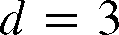
Our investigation of the MHP utility function was conducted with a spatially explicit agent-based model. This approach is very close to Schelling's original model and will allow for direct comparison. The model begins with a grid corresponding to the largest spatial area under investigation, which we will call a virtual city. This virtual city is composed of cells that we can think of as addresses. In our models, there are 1,225 cells arranged on a 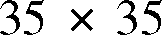 grid. This grid is wrapped around a torus to prevent edge effects. On to this grid, we randomly place 498 agents. In cases where two agents occupied the same positions, we reoriented one of the overlapping agents, by having it find a new location at random.
Each agent has some fixed property p, which, following Schelling, we can think of as race, first language, or some other (unchanging) observable property. The simulations reported here all consider cases in which agents have one of three possible values of this property, designated as types 1, 2, and 3. In all simulations, these types are evenly distributed among the 498 agents, yielding 166 agents of each type.Footnote 5
In addition to its intrinsic properties, each agent also has a radius of vision, r, within which other agents can be seen. The value of r defines the agent's perceived community, which may range in size from the agent's closest neighbors (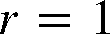 ) all the way up to the entire grid (
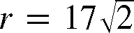 , which is approximately 24). To keep the analysis simple, every agent is given the same value for r in each simulation. This corresponds to 498 overlapping communities, each with radius r.
Given that this is an agent-based model, each agent implements a movement strategy based on an individual utility function. If  denotes the number of agents of type p in agent a's community and if (i, j, k) denotes some permutation of (1, 2, 3), then the MHP utility function,
 , for each agent a of type i is defined to be a satisficing utility of the following form:Footnote 6

Hence an agent a of type i will move to new position whenever 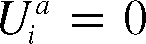 .
The basic structure of our iterative simulation model is that at the beginning of each model iteration we determine the current value of  for every agent a of type
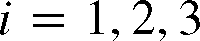 . If
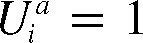 , then agent a does not move. If
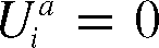 , then agent a moves according to the following rules:
1. Choose a random heading.
2. Walk forward n steps, where n is a random number between 1 and 10.
3. Determine whether any agent occupies the new grid cell. If so, return to step 1.
4. If not, occupy the center of the new grid cell.
In Schelling's own models, the movement order was decided either by starting from the center and working outward or by starting from the upper-left corned and sweeping right and down (Schelling Reference Simon1971, 148). In our models, we simulate a parallel process by randomizing the order of moves on each round. Also, Schelling had his agents move to the nearest empty square, while our procedure does not always guarantee this. The model itself is iterated repeatedly until either an equilibrium state is reached (where every agent has achieved an MHP utility of one) or else a time limit of 1,000 model iterations has elapsed.
For the analysis presented here, we consider instantiations of the model with community sizes ranging from 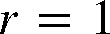 to
 in increments of 0.5. This covers the range from just under the size of the Moore neighborhoods in Schelling's model to just over the size of the entire virtual city.Footnote 7 For each community size, we ran 100 repetitions, each starting from a different random configuration of the 498 agents on the grid. We also constructed a comparison set of 100 random benchmark configurations, each generated by a random initialization of our model without running the decision procedure.
For the purposes of later analysis, a coordinate file was recorded for each simulation that gives the location of each agent and its type. In all the analyses discussed in subsequent sections, we arbitrarily chose a single type of agent for analysis and studied the extent to which this agent type exhibited either attraction to or segregation from the other two types.
3. Analysis of Segregation
Based on these simulations, our main finding is that, starting from random configurations, the equilibrium outcomes for most parameter values exhibit spatial segregation between agent types. The degree of segregation, however, depends crucially on the radius of vision r. When r is below 4.5, segregated clusters are extremely small and only exist as transients, not equilibrium states. Once we move to larger values of r, agents segregate themselves into increasingly larger clusters. It is only when r encompasses almost the whole population for each agent that segregation starts to decrease, and it eventually disappears when all agents are visible to one another. This suggests that in the current model, segregation is driven by agents having some, but not full, information about the wider community beyond their immediate neighborhood.
3.1. A Scale-Sensitive Test of Segregation versus Attraction
Given the assumed symmetry among agent types, our analysis of segregation focuses only on a single type (type 1), now designated as the target population of agents (labeled 1). Types 2 and 3 are then combined into a single reference population (labeled 0).Footnote 8 In this context, the most widely used test of attraction versus repulsion (segregation) between such spatial point populations is based on cross-K-function statistics, which formed the natural starting point for our analysis.Footnote 9 For each given community size, r, the cross-K-function value, K(d; r), denotes the expected number of reference individuals (per unit area) within distance d of a randomly selected target individual. These statistics are designed to detect either attraction or repulsion (segregation) between the target and the reference populations. Roughly speaking, an unusually small (large) value of K(d; r) is taken to indicate significant segregation (attraction) between these populations at scale d.
However, while tests based on cross-K-function values did indicate the presence of significant segregation over a range of spatial scales, visual comparisons between typical equilibrium patterns and test results showed that these statistics sometimes failed to detect segregation that was readily apparent (especially for extreme values of r). Further analysis suggested that the main reason for this is that values K(d; r) focus only on the numbers of reference agents within distance d of a given target agent and ignore the presence or absence of other target agents. Hence, segregated clusters of similar agents were often missed.
This led us to consider a modified test statistic that incorporates counts of both types of agents. The particular form of this statistic (which is tailored to our current simulation model) is based on the observation that if the three identical populations of agents were randomly distributed throughout the virtual city, then in any given subregion, one would expect to find about the same numbers of each agent type. Hence, if we now let 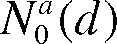 denote the number of reference agents within distance d of a given target agent, a, and let
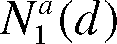 denote the number other target agents within distance d of a, then under complete randomness one would expect
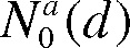 to be about twice as large as
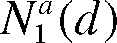 . Thus, our test statistic is designed to estimate the expected difference,
 , which should be about zero under complete randomness. However, to be precise, one must consider the conditional expectation,
 , given the inclusion of target agent a. It is shown in the appendix that if
 denotes the number of distinct cells within distance d of any given cell, that is, the d-neighborhood of this cell (which must be the same for all cells by our torus construction), then a correction term,
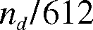 , is required in order to ensure zero expectation with respect to every d-neighborhood (given our specific population sizes of each agent type). With this correction, the desired modification of cross-K-functions for our current purposes is based on the conditional expected local differences defined for each agent, a, and distance, d, byFootnote 10

It is shown in the appendix that under the null hypothesis of randomly located agents, 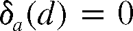 for all d-neighborhoods.Footnote 11 Hence, in each d-neighborhood of agent a, positive (negative) values of
 are associated with larger (smaller) numbers of reference agents relative to target agents than would be expected under randomness.
Observe next, from the identity of MHP utility functions for all agents and the complete symmetry of all cell locations on the torus, that this conditional expectation must be the same for all target agents. Hence, the specification of a particular agent, a, in (2) could in principle be dropped. But for expositional purposes, it is most convenient to eliminate dependency on a by averaging. Thus, we now focus on the expected local difference across all target agents,  , at scale d, as defined by

As a parallel to cross-K-functions, these expected local differences can equivalently be interpreted as values of (2) for a randomly sampled target agent.
Before developing tests based on these indexes, it should be noted that for d equal to the community size, r, there is a close relation between  in (2) and the values of a's MHP utility in (1). In particular, since
 for each agent, a, in equilibrium, and since the correction term (
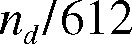 ) tends to be relatively small by comparison,Footnote 12 one can expect to find positive values of
 in equilibrium. So at equilibrium, one should not be surprised to find a substantial degree of attraction at the community scale, r, which is of course precisely what individual agents are trying to achieve. Thus, our main interest focuses on the consequences of this behavior for segregation or attraction at scales,
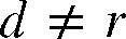 .
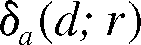
With these definitions and informal observations, we can now formalize our testing procedure as follows. If at each community size, r, we let 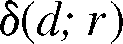 denote the expected local difference in (3) for MHP processes under r (with corresponding conditional forms,
 , in eq. [2]) and similarly let
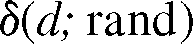 denote the expected local difference in (3) for the random benchmark process defined above, then our testing procedure focuses on the difference between these mean values,

at each scale, d, and community size, r. Given the above interpretation of expected local differences, positive (negative) values of 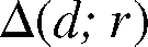 can also be taken to imply more attraction (segregation) between agent types at scale d than would be expected under the random benchmark process. A test of the statistical significance of these Δ-values can thus be implemented in terms of a standard difference-between-means test.
To carry out such a test, we performed  simulations of the MHP process under each community size, r. If for each simulation
 we let
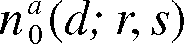 and
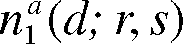 denote the observed values of
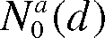 and
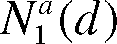 in that simulation and let

denote the corresponding (one-sample) estimate of 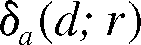 , then the resulting estimate of
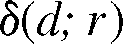 under community size r is given by

Similarly, for N parallel simulations of the random benchmark process, one can construct corresponding estimates:

At this point it should be noted that the individual estimates 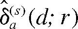 (respectively,
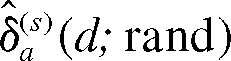 ) are not independent within a given simulation (since d-neighborhoods can overlap one another). However, the estimates
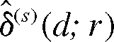 (respectively,
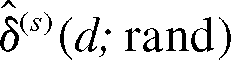 ) for separate simulations, s, are independent by construction. Hence, these can be regarded as N independent random samples of mean estimates from both the MHP process and the random benchmark process.
Given this independence property, it follows that if the resulting sample estimate of 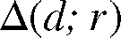 for each simulation, s, is denoted by

then the grand mean across all simulations; that is,
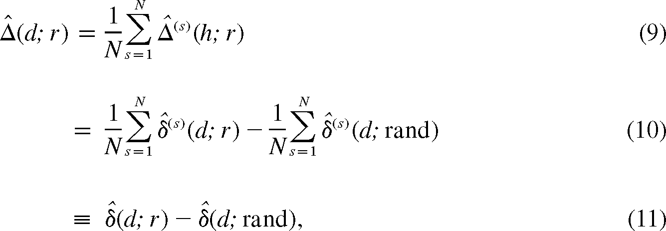
yields an appropriate test statistic for discriminating between the MHP and the random benchmark processes. In particular, this statistic satisfies the conditions for a Welch-Satterthwaite (WS) difference-between-means test that allows for possibly different variances between these two statistical populations.Footnote 13
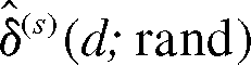
To carry out this test, we first calculated the sample means for the MHP process in (6) and the random benchmark process in (7) for each simulation. This was accomplished with a program (written in Matlab by one of the authors) that calculates 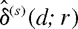 and
 at each scale, d, in each simulation, s. Here it should be noted that while community sizes, r, are allowed to range up to the maximum torus distance of approximately
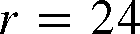 , we restrict the scale values, d, to lie in the range
 . The reason for this is that our torus approximation of d-neighborhoods on large planar grids breaks down for distances greater than half the width of the original (
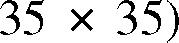 square, that is, for
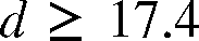 .Footnote 14 These computed sample means formed the basic inputs for the WS test conducted at each scale,
 , and community size,
 .
The test results were determined by calculating the t-values for 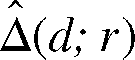 and applying the WS approximate t-distributions for two-sided tests of the null hypotheses
 for each choice of r and d. For all practical purposes, none of these t-distributions were distinguishable from the normal distribution at the given sample sizes (of
 for each population). So our formal rule was basically to conclude significant attraction for t-values above 1.96 and significant segregation for t-values below −1.96. But since the computed t-values ranged so far outside this interval, it proved to be more informative to plot these t-values directly and simply indicate the critical interval
 on the graphs.Footnote 15
3.2. Test Results
To summarize our test results, we begin by observing that for all community sizes,  , the simulations always settled to an equilibrium state. The only exception is the extreme full-visibility case of
 , where by definition no equilibrium is possible (since no agent can be in a strict minority). Moreover, the test results showed that these equilibrium states for community sizes
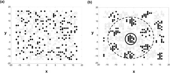
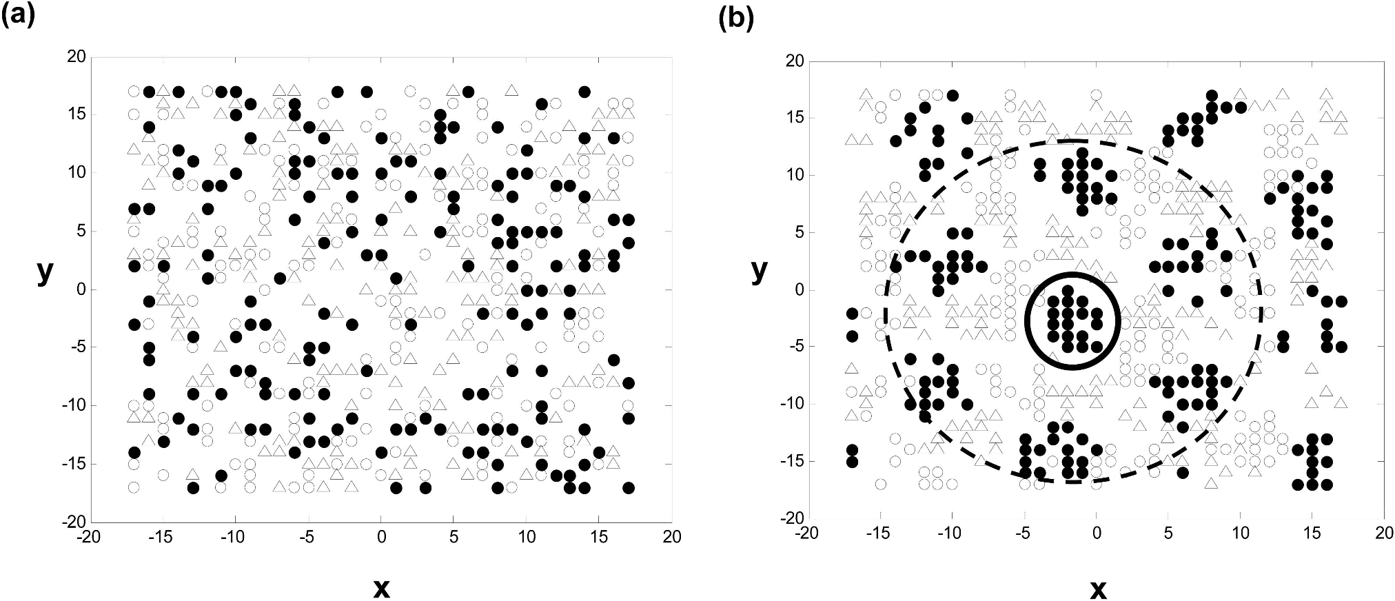
 always involve significant segregation below a certain critical scale, dr, depending on r. So even though agents are maximizing their MHP utilities (i.e., are in minorities less than one-third of their current community populations), they nevertheless find themselves in segregated neighborhoods at all scales not exceeding the critical scale, dr, for their radius of vision, r. This is illustrated in figure 1b for a community size of
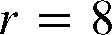 , with critical scale
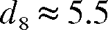 . Here, the filled circles denote locations of target agents (type 1), and the locations of reference agents (type 2 and type 3) are denoted by open circles and triangles, respectively. (The large circles in the figure will be discussed below.) Here it is visually evident that each agent type exhibits clustering that results in segregation at certain scales, as will be verified by the test results below. For purposes of comparison, figure 1a shows the initial realization of the random benchmark process leading to the equilibrium pattern in figure 1b.
Example equilibrium pattern (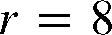 ). a, Initial random configuration; b, final equilibrium pattern.
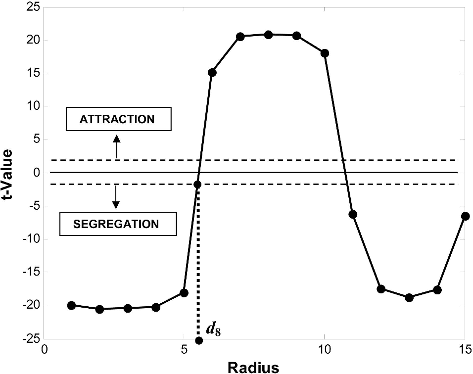
Turning now to the test results themselves, it is again useful to illustrate these findings for the case of community size 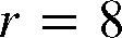 , in figure 1b. The full plot of t-values for all relevant scales,
 , is shown for this case in figure 2. Here the relatively narrow width of the critical interval
 (indicated by the horizontal dashed lines in the figure) shows that there is a strong degree of statistical significance in both the regions of attraction and the regions of segregation in the figure.Footnote 16
Plot of t-values for community size 8.
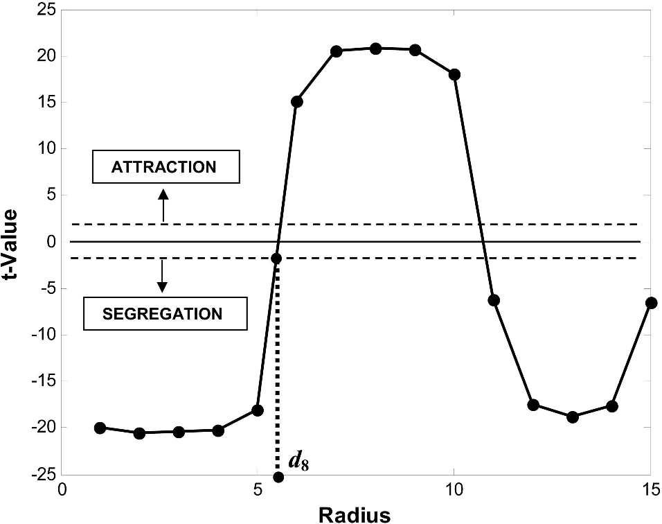
As for the shape of the plot in figure 2, notice first that as predicted above (in the discussion of expected local differences), there is a peak of very significant attraction at precisely scale  , reflecting the MHP utility-maximizing behavior of all agents.Footnote 17 More important for our current purposes is the lower end of the graph, where there is seen to be significant segregation between agent types at all scales,
 .Footnote 18 Here segregation appears to be most significant at a scale of about
 . Visually this corresponds to circular neighborhoods of radius 3 about each cell, as illustrated by the solid circle near the center of figure 1b. This particular neighborhood is seen to be just large enough to cover the cluster of target agents (filled circles) shown in the figure. More generally, the most significant scales of segregation (below the critical scale, dr) for each community size,
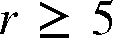 , tend to reflect the cluster sizes of agent types seen in typical equilibrium patterns for that community size.Footnote 19 Thus, while figure 1b shows only one instance of a simulated equilibrium pattern for community size
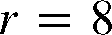 , it helps to illustrate the broader statistical results summarized in figure 2. Note finally that beyond the attraction peak at
 , there appears to be a second peak of significant segregation at about
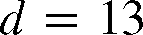 . But further analysis shows that secondary peak is essentially a reflection of the regularly spaced clusters of agents at smaller scales. For example, the dashed circular neighborhood of radius 13 that is concentric with the smaller circle in figure 1b is seen to be just large enough to include the second wave of target-agent clusters adjacent to the central cluster shown. Hence, the concentration of target agents at this scale is a consequence of a similar concentration at smaller scales.
To analyze further properties of these statistical results, it is useful to distinguish three ranges of community sizes, r. The first is the minimal range, involving community sizes 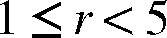 , in which equilibria do not always occur. The second is the intermediate range,
 , which covers the most interesting cases for our purposes, and the third is the maximal range,
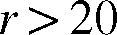 , which exhibits behavior somewhat different from that of the intermediate range. Here we begin with the most important intermediate range and then consider each of the extreme ranges in turn.
3.2.1. Intermediate Community Sizes
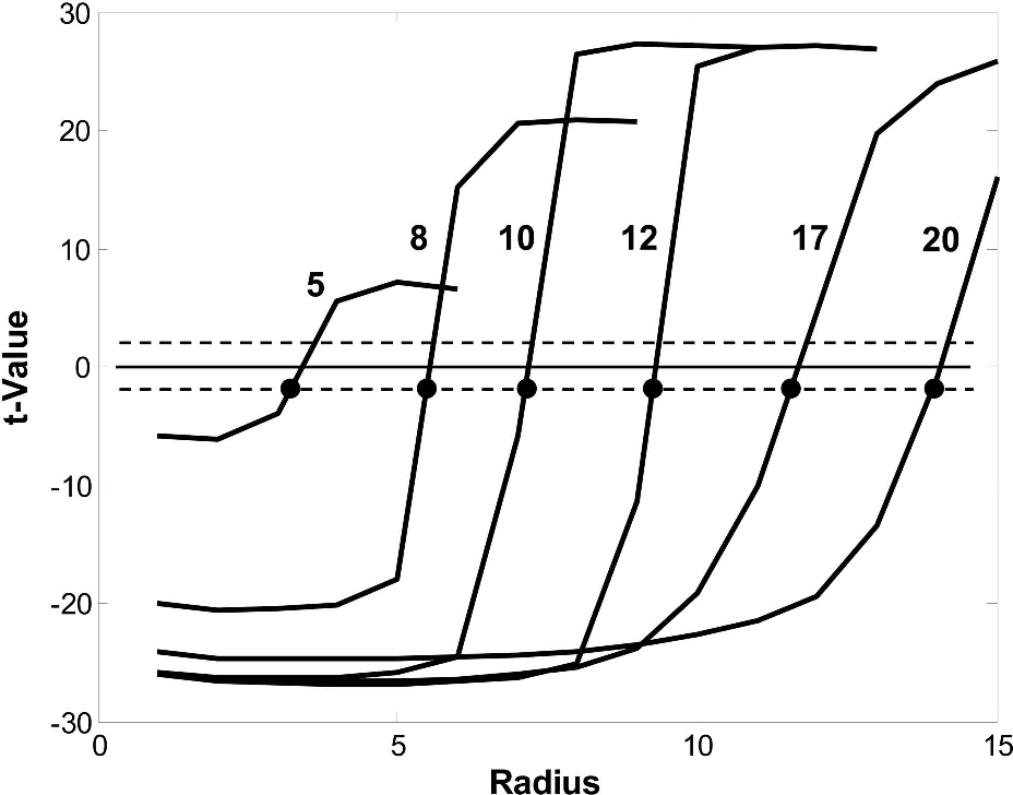
The key feature of the intermediate range,  , is the relation between each community size, r, and its associated critical scale, dr. Specifically, as the radius of vision increases, the critical scale for segregation also increases. This is illustrated in figure 3, where the t-values are plotted for selected values of intermediate radii (5, 8, 10, 12, 17, 20)Footnote 20 and where each curve is numbered by its associated community size.
Community sizes 5–20.
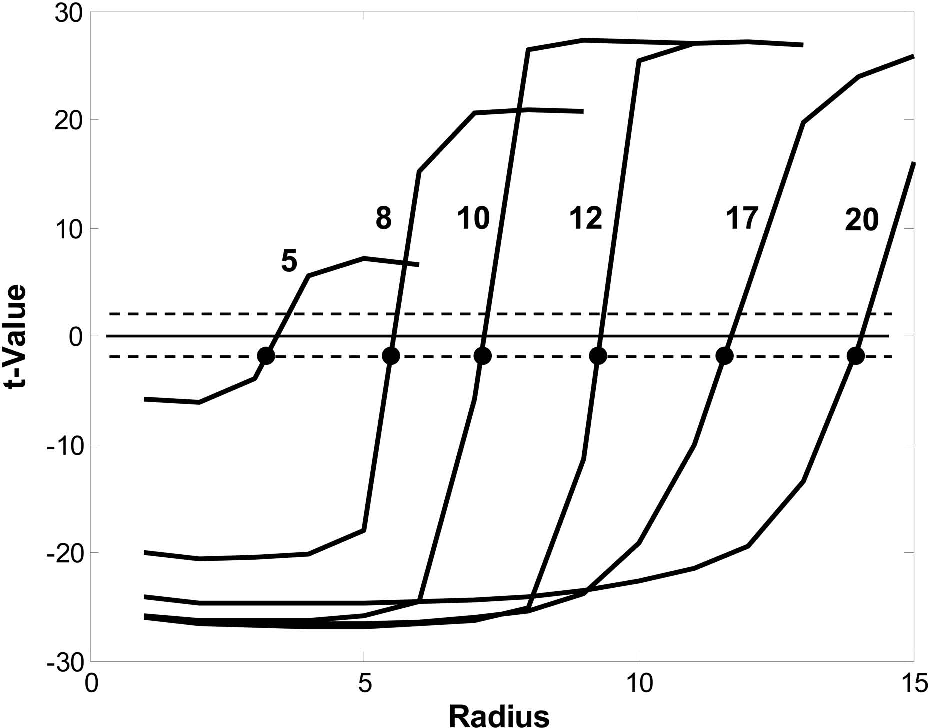
For the sake of visual clarity, only the most relevant portion of each curve is shown, specifically the t-values at all scales, 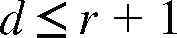 , for each community size, r. For example, the curve shown for community size
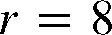 is seen to be the lower portion of the same t-value curve in figure 2. By definition, the critical scale, dr, for each community size, r, is seen to be the scale at which the associated t-value curve first intersects the critical interval from below (shown by a filled circle on each curve). So on curve
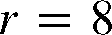 , the filled circle is seen to be at scale
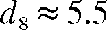 . Hence, the steady increase in these critical scale values is easily seen by the progression of these intersection points.
Estimating the number of agent clusters
To obtain further statistical insight into this segregation phenomena, we constructed a program that attempts to identify the number of spatial clusters in the target population. This program involves two stages. First, the equilibrium configuration of n individual target agents was successively grouped into smaller numbers of clusters by continually adding closest clusters (where distance between clusters was measured as the distance between their closest points). This hierarchical clustering procedure was continued until the n points corresponding to the target population were reduced to a specified cutoff number of clusters (which was set sufficiently low to include all clustering levels of potential interest).Footnote 21
With a cluster hierarchy in hand, the second step was to determine the best number of clusters with which to group the target population. This number was not always obvious on visual inspection and exhibited substantial variation between simulations (with different initial random configurations of agents). After considerable experimentation, it was found that two criteria seemed to place reasonable bounds on the number of clusters observed visually. The first criterion (which focuses on achieving compact groupings within each cluster) is to find the cluster configuration that minimizes the mean-squared distance of points to their respective cluster centroids.Footnote 22 Since this criterion value, C 1, for each cluster partition is always decreasing in the number of clusters, it was decided to compare observed values with those expected under random configurations. Here cluster hierarchies for 1,000 random configurations were constructed and used to estimate the sampling distribution of C 1 under randomness. When observed criterion values, C 1, are replaced with their z-scores, Z 1, under this distribution, the cluster number with the minimum Z 1 value can be interpreted as that for which C 1 is most significantly lower than would be expected under randomness. The second criterion (which focuses on achieving good separation between clusters) starts by computing for each cluster the shortest distance between points in the cluster and points outside and then finds the cluster configuration that maximizes the mean of these shortest distances for each cluster. Since these values, C 2, are also monotone decreasing in the number of clusters, the same random cluster hierarchies were used to construct a sampling distribution of C 2 under randomness. When observed values C 2 are replaced by their z-scores, Z 2, the cluster number with maximum Z 2 value can be interpreted as that for which C 2 is most significantly higher than would be expected under randomness. As stated above, the optimal cluster numbers, N 1 and N 2, produced by these two criteria tended to place reasonable bounds on the number of clusters observed visually over a wide range of examples. Hence, our final representative cluster number, N, was obtained by taking the average,  , of these two optima.
To analyze these cluster numbers, we simulated 1,000 equilibria for each possible community size,  , and constructed corresponding cluster numbers, Nir, for each simulation
 . But in order to interpret these results, it is important to note that cluster numbers by themselves are only meaningful relative to the particular size of the torus approximation used. Hence, it was deemed to be more appropriate to convert each cluster number, Nir, to a corresponding average cluster size,
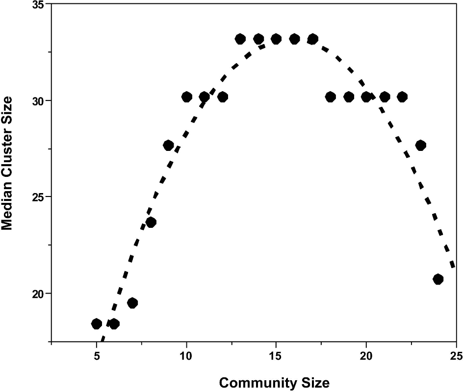
 , in terms of target agents per cluster.Footnote 23 In particular, the average size of these clusters relates more directly to the degree of segregation exhibited by the agents. In figure 4, the median of these cluster sizes
 is plotted for each community size,
 .
Equilibrium cluster sizes.
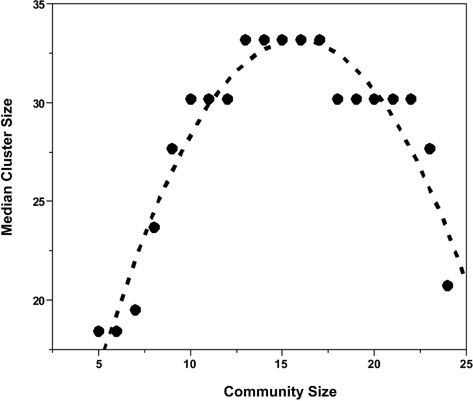
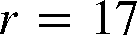
The step-function nature of the plot is a consequence the underlying discreteness of possible cluster numbers. But even with this lack of smoothness, the regularity of its overall pattern is evident.Footnote 24 In particular, median cluster size (degree of segregation) first increases with community size up to a radius of about 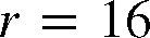 and then decreases with all larger community sizes (as emphasized by the simple quadratic fit shown as a dashed curve). This is in rough agreement with the segregation results above (in terms of critical scales), except for the slight decrease in cluster size from
 to
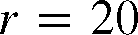 . But even here it should be borne in mind that this decrease from about 33 to 30 agents per cluster corresponds to the smallest possible increase in median cluster numbers from 5 to 5.5.Footnote 25 So substantial decreases in cluster sizes are only seen to occur beyond
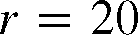 .
It should also be noted that the cluster identification procedure underlying this plot is far less precise that the statistical significance results above. But in spite of its lack of precision, this procedure served to identify one additional feature of these equilibrium patterns that was entirely missed by our difference-between-means tests.
A secondary equilibrium mode
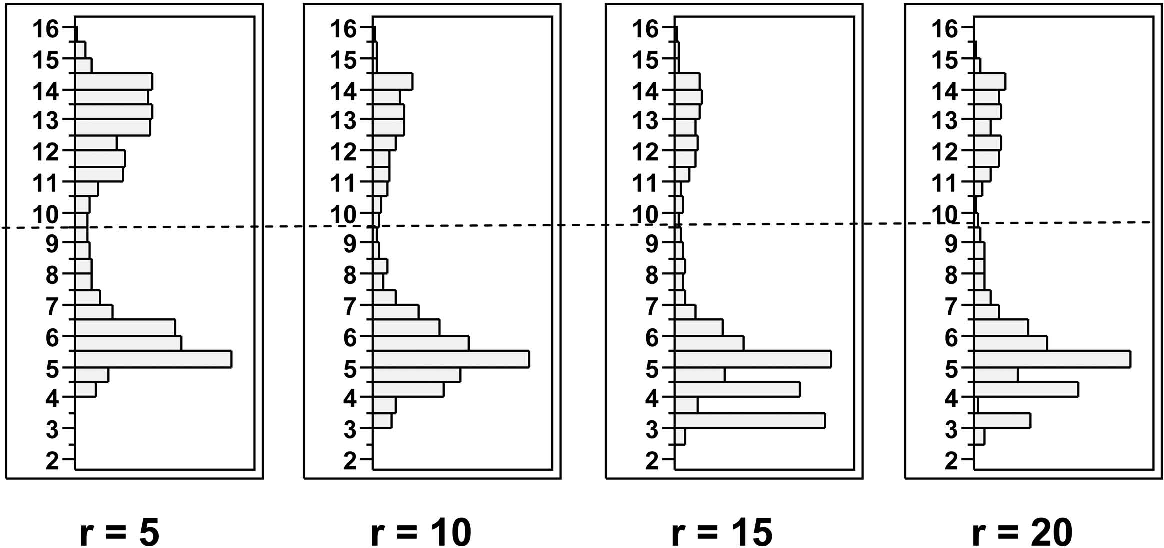
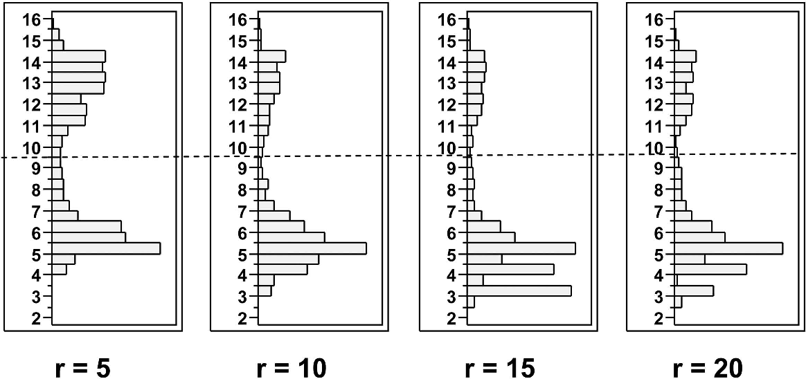
The histograms of cluster numbers identified at each community size revealed that there are actually two modes of equilibria: a primary mode and a secondary mode. In figure 4, we have displayed these histograms for four community sizes,  , that are typical of the full range of sizes.
Here, the primary mode (small numbers of clusters) corresponds to the segregated equilibria that are the focus of this article, and the secondary mode (large numbers of clusters) corresponds to equilibria in which essentially no segregation is evident.Footnote 26 One should hasten to add that, except for the most extreme community sizes (close to either 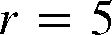 or
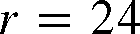 ), the primary mode involves about 75% of all equilibria. But nonetheless, this secondary mode is of some interest.
First of all, while it is not difficult to construct rather uniform equilibrium configurations in which all agents are maximizing MHP utility, it was not clear to us that such equilibria could be even locally stable. However, these results show that many are. Moreover, the presence of such equilibria suggests that unless the initial random configuration involves some minimal degree of clustering (as generally seems to be the case), segregation may fail to emerge in equilibrium.Footnote 27 It is also of interest to note that unlike the primary mode, these nonsegregated patterns appear to be very insensitive to community size. As shown by the dashed line in figure 5, this mode always ranges between about 10 and 16 clusters, with a mean around 12.5. Hence, these dispersed patterns appear to exhibit roughly the same degree of agent heterogeneity at all scales.
Cluster size distributions.
Finally, in view of the nonsegregated nature of this secondary mode, it is important to ask whether the inclusion of this mode might distort the relation of cluster sizes to community sizes occurring within the more important primary mode. This can be checked by including only cluster numbers, Nir, within in the primary mode (i.e., 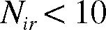 ) and constructing a median plot paralleling figure 4. Given the invariant shape of this secondary mode across community sizes, it is perhaps not surprising to find that the primary-mode plot is qualitatively almost exactly the same. Hence, the only effect of this secondary mode is to inflate the level of median cluster numbers obtained. But since the ultimate effect of this inflation is to yield lower (more conservative) estimates of the degree of segregation present, we have chosen to show only the combined plot.
3.2.2. Minimal and Maximal Community Sizes
When agents’ community size is very small 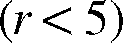 , the model fails to reach an equilibrium state in which all agents have maximal MHP utility. Nevertheless, the underlying dynamics of the model continue to exhibit a nonrandom spatial structure that we set out to investigate.
We began with 498 agents of three types distributed randomly over our toroidal grid. Like in the procedure used to study medium neighborhood sizes, we investigated 100 simulations for each neighborhood size corresponding to a different initial distribution of agents. Since the simulations never reach equilibrium, we chose to sample the pattern reached after 1,000 iterations of the model. This set of 100 samples was then compared to a set of 100 randomly generated distributions of agents on the grid using precisely the same procedure as above. In particular, we computed the appropriate  values in (6) and (7) above for each simulation,
 , and then tested for significant differences between them.
For these small neighborhoods, we found patterns that correspond to the secondary equilibria discussed above. Visually, this appears as very small clusters—more structured than completely random but not statistically significant. These clusters are unstable, as the agents in them all have low utility and will continue to move, seeking higher utility. Nevertheless, they persistently reappear as the model is iterated.
Finally, for large community sizes (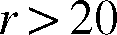 ) we found that equilibria continued to emerge all the way up to the maximal community size of
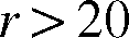
 (in which no equilibrium is possible). However, the critical scales, dr, for significant segregation in such equilibria began to diminish. This is also seen in figure 4 above, where median cluster sizes diminish rapidly for
 . A possible explanation for this diminishing effect is given in the next section.
4. Discussion
Schelling's original result was striking but perhaps not altogether surprising. While the degree of segregation observed in his model is far higher than any individual's preference for homogeneity, agents still desired some degree of homogeneity in their neighborhoods. In our model, agents want to be surrounded by agents that are different from themselves. So why does segregation still arise in the model?
We believe that the result can be explained by careful consideration of the microdynamics of MHP models. Consider a model like ours with only two types of agents, and start with a population of only two agents (a and b) of the same type in close proximity. Because they have maximally heterogeneous preferences, these agents will be repelled from each other until they move outside each other's community. This repulsion, however, begins to be modified as additional agents are added to the model.
For example, suppose now that three new agents (c, d, and e) of the opposite type are placed in close proximity to the original two. Agents a and b will still repel each other but will also both be attracted to c, d, and e because they are different in type. This means that a might now tolerate being close to b because there is a chance to be in a strict minority relative to c, d, and e.
A more formal way of thinking about these dynamics is to consider the informational state of the agents as they make decisions. As each agent relies on exactly the same decision rule and utility function, only two factors can cause agents to make different movement decisions: their agent type and their information about the locations and types of other agents, which we call the agent's information set.
Consider how these two factors interact. Each agent's information about its surroundings is strictly defined by its radius of vision. As such, this information set is position dependent. A consequence of this position dependence is that as two agents move closer together, their information sets become increasingly correlated. When they are adjacent, their information sets are very nearly identical. For two agents that are of different types, this near identity of information sets will not necessarily lead to identical behavior because their types will lead them to have different interests. However, for two agents that are of the same type, we should expect their movement decisions to be highly correlated. Thus, correlations in information sets will correspond to correlations in decisions about where agents want to move. As the relocation process continues, local groups of target agents will tend to move toward similar positions. This will in turn lead to further information convergence about the agents in their respective neighborhoods. In this way, similarity of information sets becomes its own attractor.
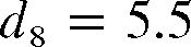
This attractive power of informational similarity is possible in our model because of the focus on communities rather than neighborhoods. Neighborhoods are fairly small and can contain relatively few agents. However, depending on their radius of vision, the communities relevant for agents can be much larger geographically and, hence, can contain many more agents. For example, in our current model suppose we let Sr denote the set of cells within distance r of any given cell and consider vision radius 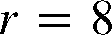 (as discussed in sec. 3.2 above). Then it is readily verified that the relevant community, S 8, for any target agent, a, can contain as many as 197 agents. In this context, if we consider a neighborhood, S 4, of radius 4 about agent a (which is less than the critical scale of
 ), then it can also be verified that S 4 can contain at most 49 agents. Hence, even if all agents in neighborhood S 4 are also target agents, it is still quite possible that this population is a strict minority in a's community, C 8. Moreover, as vision radius r increases, the maximum population size of Cr grows in proportion to r 2.Footnote 28
More generally, considerations of both (i) neighborhoods versus communities and (ii) the overlap between agents’ information sets offer possible explanations of the systematic changes in critical scales and median cluster sizes as vision radius changes. First, for small radii, r, since the communities of agents are not much larger than their immediate neighborhoods, no equilibrium is possible in which target agents have even a few other target agents as neighbors. It is only when r becomes sufficiently large relative to local neighborhoods that sizable clusters of target agents are possible in equilibrium. Moreover, as r increases, the overlap between the communities (information sets) of adjacent agents must also increase, so that adjacent agents are more likely to share minority positions in their similar communities. These two factors together thus help to account for the initial growth in both critical scale values and median cluster sizes as r increases from small values.
At the other extreme, recall that when r is maximal and all agents are visible to one another, no agent can be in a strict minority. In this extreme case, target agents will be equally dissatisfied at all locations. In particular, locations near target agents will be no more attractive than other locations. But as r decreases from this extreme, information sets will differ between locations and, in particular, will now be more correlated at locations close to one another. So as the system approaches equilibrium, with many target agents already satisfied, it is more likely that locations close to them will also yield satisfaction for relocating target agents. So again one can expect to see larger clusters of target agents appearing in equilibrium as r decreases from its maximal value.
5. Conclusions
We set out to investigate the robustness of Schelling's famous segregation result, subjecting it to the most stringent test that we know. Our model shows that MHP utility functions, where agents want to be in the smallest minority, can themselves create segregated clusters. So long as agents have only partial information about their entire city, and consider their community to be a few blocks in size, we find robust segregation in equilibrium.
This result, combined with those previously established, shows the overwhelming prevalence of segregation when agents base their decisions on racial preferences. So long as agents all base their decisions on the same property, regardless of their attitudes toward it, we will tend to find segregation in a population. In this model, we aimed to provide the strongest possible test of this hypothesis, by having agents actively seek out those that are different from themselves. However, by adding the very weak, realistic assumption that people care about their community rather than just their immediate neighbors, we find that individuals still typically end up in a segregated state.
This result tells us two things: First, it tells us that Schelling's original model is extremely robust to various kinds of perturbation. Second, it tells us that because of this robustness, we have a single macrobehavior that could be supported by a wide variety of underlying micromotives. Let us consider each in turn.
The robustness of Schelling's original model can be best explained by the fact that the underlying dynamic relies only on a tipping phenomenon. So long as all the agents have the same structure to their preferences, initial innocuous movements will quickly cascade across the entire population, and we have segregation as an absorbing state of the model. In our model, we saw that informational similarities were sufficient for this cascade to occur. Informational similarities result in highly correlated movement decisions, and as agents move more toward one another, their information sets become increasingly similar. This is a rather different dynamic from the standard Schelling model. In the original model, we get cascades of movement because agents were weakly repelled by agents of a different type, and once enough of their fellows have moved out of their neighborhood, their threshold for happiness is no longer met, and they move themselves. This creates a separating equilibrium, in which each type is most easily satisfied by being among its own. Nothing in that model relies on informational similarities. But in each model, a cascade of segregation occurs and quickly takes over the population.
This robustness reveals why Schelling's initial insight is so essential. We cannot argue from the observation of a macrobehavior to an understanding of its microfoundations without a great deal of additional investigation. While determining whether a model's results are robust is an essential component to most model validation, robust models can pose their own unique scientific challenges. When we have a model with very fragile results, where the phenomenon under study only manifests itself under quite limited conditions, we can often be in a superior epistemic position. If the fragile model's assumptions are appropriately realistic and calibrated against empirical information, then we have a much better chance of having captured the precise underlying dynamics for the macrophenomenon in question. This suggests that intervention strategies can be more easily studied and implemented. However, with robust modeling results the same phenomenon can be overdetermined by competing explanations. In cases of extreme robustness, such as with the Schelling result, our epistemic position can actually be weakened. As such, we learn less about the empirical phenomenon than we do in the fragile cases; we cannot identify what microdynamic is correct without further study.
Although segregation is extremely robust in the family of Schelling-like models, not all cities are massively segregated, and perhaps some cities are well integrated. This leads to the observation that these models do not capture the precise population dynamics unfolding in cities, which is unsurprising given the models’ simplicity. However, they remain important tools not only for a fundamental understanding of population dynamics but also for thinking about the effects of potential policy interventions.
Segregation's robustness suggests that most policy interventions are likely to fail to prevent one of the many possible microdynamics from taking over and continuing to drive segregation. But this prediction is testable. If we can find and study full or partially integrated communities, then we would discover that the Schelling model and its variations fail to capture some feature of the real world that is essential for a proper understanding of the segregation phenomenon. So while we have seen that the original Schelling model is quite robust, it is possible that it is too robust. Given its strong predictions of the near certainty of segregation, this robustness makes it easy to mount challenges to the completeness of the model.
Appendix
We derive the normalization term required for the zero-expectation condition that 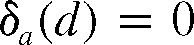 holds for all d-neighborhoods. In particular, we calculate the conditional expectations of both
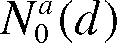 and
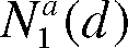 given the presence of an agent, a, and use these to normalize the expected difference,
 . To do so, we begin by observing that the null hypothesis of random assignments of each agent type to distinct cells on the torus grid of 1,225 (352) cells yields a standard “urn sampling” problem with associated hypergeometric distributions for the random variables,
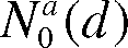 and
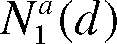 . But given the population sizes of 166 agents of each type, these distributions are well approximated by binomial distributions (which technically involves sampling with replacement, where more than one agent can in principle occupy the same cell). Given this approximation, and recalling from the text that nd denotes the number of distinct cells within distance d of the cell occupied by agent a (which is the same for all cells), the conditional expectation of
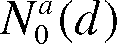 given the presence of a is simply

where  is the probability that any given cell other than a's cell is occupied by a reference (type 0) agent. Similarly the conditional expectation of
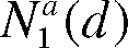 given the presence of a is of the form

where  is the probability that any given cell other than a's cell is occupied by one of the other 165 target (type 1) agents. Thus, it follows at once that
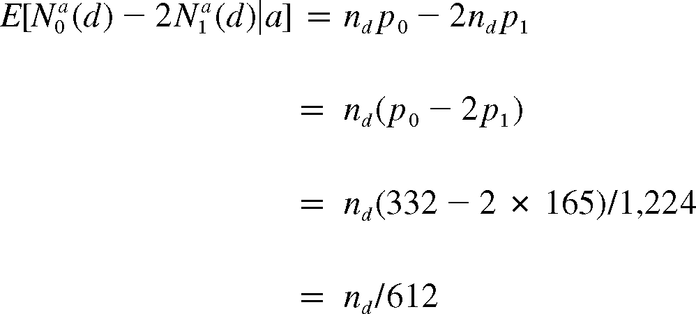
and hence from (3) that for all d,

must hold under these assumptions.
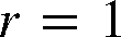 corresponds to a rook neighborhood (analogous to rook moves in chess) consisting of a cell together with the four cells sharing one of its faces. In these terms, a Moore neighborhood is also called a queen neighborhood since it includes the additional four cells sharing corners with the given cell.
 for each agent, a, in the target population depends only on the total size
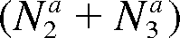 of the reference population in a's current community, there is no need to distinguish between agent types within this reference population.
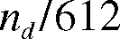 , cancels out and has no influence on the tests to be conducted.
 , it follows by definition that
 . This in turn implies that
 and, hence, that the effect of this correction is small relative to the expected counts involved.
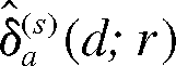 , are generally not normal, their sample means,
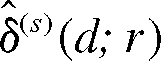 , were confirmed (by Shapiro-Wilks tests) to be sufficiently normal for testing purposes. Normality in this case can also be justified on theoretical grounds from the well-known asymptotic normality properties of sample means for locally dependent data.
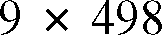 agents. But while the number of target-agent clusters would increase ninefold, the average cluster size in terms of target agents would remain the same.
 , that the closest value above 5 is
 .
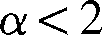 . In these instances, simulation results are qualitatively similar to the no-discounting case.