1. Introduction
Bilateral teleoperation has begun to formally spread during the mid-20th century [Reference Hokayem and Spong1], with exemplary cases such as Raymond C. Goertz’s master–slave architecture for radioactive material handling in 1953 [Reference Goertz2], or William R. Ferrel’s work on transmission delay in 1965 [Reference Ferrell3]. Since then, this approach has garnered escalating attention within the scientific co09unity, driving ongoing interest and development over the last decades.
Teleoperation excels by strategically addressing challenges tied to human presence. These challenges span from extreme environmental constraints [Reference Goertz2, Reference Imaida, Yokokohji, Doi, Oda and Yoshikawa4, Reference Jakuba, German, Bowen, Whitcomb, Hand, Branch, Chien and McFarland5] to logistical difficulties arising from systematic or unforeseen lack of skilled professionals in specific geographical areas, as evident in fields such as telemedicine and telesurgery [Reference Evans, Medina and Dwyer6–Reference Barba, Stramiello, Funk, Richter, Yip and Orosco8]. In such scenarios, optimal conditions can also necessitate the seamless exchange of visual, auditory, and haptic feedback from the slave device so as to mitigate the challenges related to the absence of the operator within the operation area [Reference Choi, Oskouian and Tubbs7, Reference Chu, Cui, Zhang, Yao, Tang, Fu, Nathan and Gao9]. Haptic feedback implementation has been demonstrated to optimally address to this problem [Reference Bolopion and Régnier10, Reference Bayraktaroglu, Argin and Haliyo11].
On the telesurgical field, a plethora of solutions have been invented in order to adequately address a various range of surgical interventions, such as spinal surgery [Reference Tian, Fan, Zeng, Liu, He and Zhang12, Reference Lopez, Benzakour, Mavrogenis, Benzakour, Ahmad and Lemée13], laparoscopy [Reference Rovetta, Sala, Wen, Cosmi, Togno and Milanesi14, Reference Meskini, Saafi, Mlika, Arsicault, Zeghloul and Laribi15], and cancer care [Reference Satcher, Bogler, Hyle, Lee, Simmons, Williams, Hawk, Matin and Brewster16]. In each mentioned scenario, the surgeon maneuvers a master device to monitor and control the position of an instrumented tool interacting with the patient. Often, this involves implementing a remote center of motion (RCM) constraint to minimize the surgical incision required for entering inside the patient’s body.
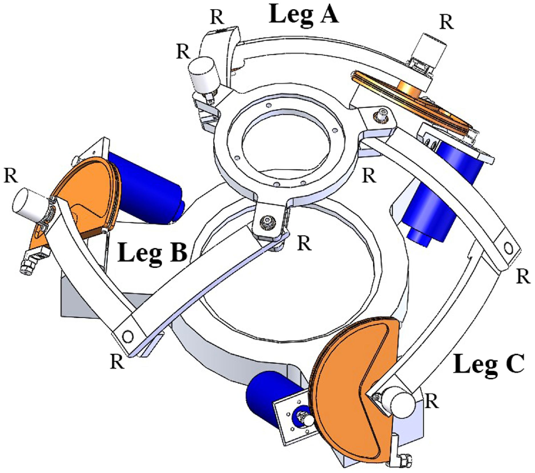
On the topic, one of the authors has already presented different spherical parallel manipulator (SPM) master prototypes [Reference Chaker, Mlika, Laribi, Romdhane and Zeghloul17–Reference Saafi, Laribi and Zeghloul20], out of many possible architectures present in literature, as in refs. [Reference Bonev, Chablat and Wenger21–Reference Zarkandi23]. The first design [Reference Chaker, Mlika, Laribi, Romdhane and Zeghloul17], as in Figure 1, consisted of three symmetrical legs composed by two links (“proximal” and “distal”) and three revolute joins (3-RRR prototype).
3-RRR spherical parallel manipulator inside solidWorks environment [Reference Chaker, Mlika, Laribi, Romdhane and Zeghloul17].

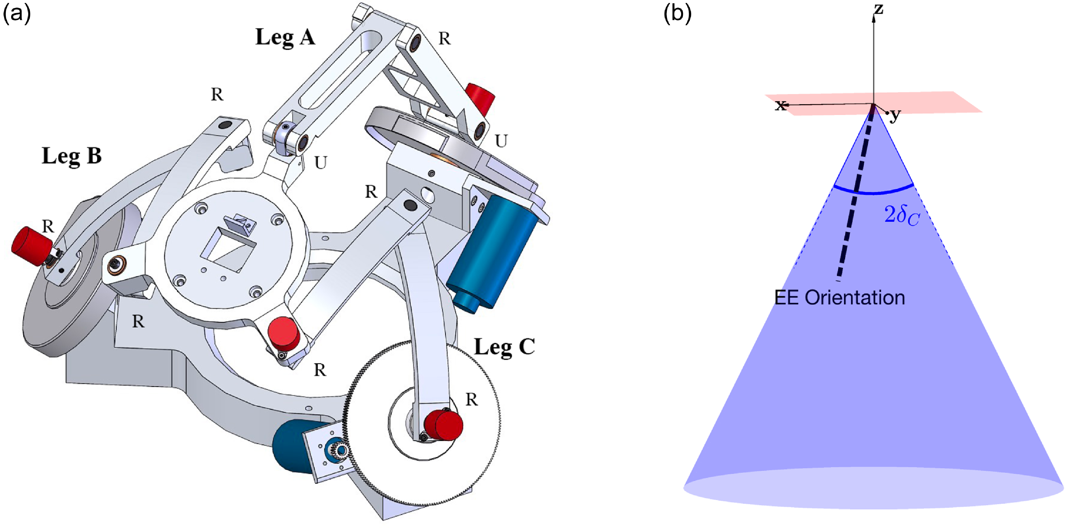
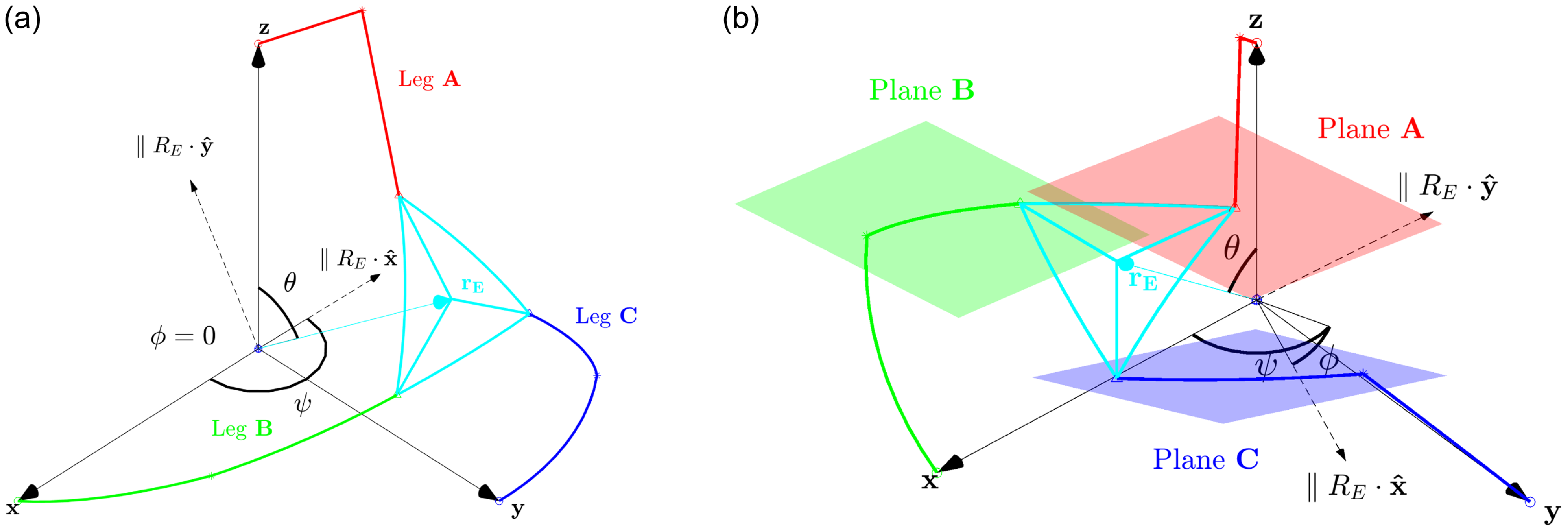
As a previous article has demonstrated [Reference Saafi, Laribi and Zeghloul18], the mentioned architecture lacked sufficient dexterity due to the presence of serial and parallel singularities of each of the three legs within the operative workspace. Other articles [Reference Saafi, Laribi, Zeghloul and Arsicault19, Reference Saafi, Laribi and Zeghloul20] have proposed and experimented on a different viable architecture, the quasi-spherical parallel manipulator (qSPM), deriving from the 3-RRR prototype by modifying the first and the last joint of one leg to be a universal joint instead of a rotational one, as in leg A of Figure 2a. This architecture was selected as it leads to a more dexterous solution, presenting singularity points further away from workspace center [Reference Saafi, Laribi, Zeghloul and Arsicault19]. The main objective of the end effector (EE) is controlling the orientation of an instrumented tool mounted on a robotic slave arm [Reference Sadeghian, Zokaei and Jazi24, Reference Trabelsi, Sandoval, Mlika, Lahouar, Zeghloul, Cau and Laribi25] and acting on an RCM conic workspace shown in Figure 2b. The architecture is actuated by three motors mounted around the absolute reference frame (RF) axes and acting on the proximal links, as highlighted by
 $A,B,C$
in Figure 2a.
The quasi-spherical manipulator (qSPM) device inside SolidWorks (a); operative workspace inside the cartesian space (b). Relevant dimensions of the device are outlined in Table II in appendix.

The previous scientific production [Reference Saafi, Laribi, Zeghloul and Arsicault19, Reference Saafi, Laribi and Zeghloul20], nonetheless, did not take into account the actual reachable workspace of the robot, that is, the workspace accessible from the central position without either crossing singularity or self-collision. Around the matter of self-collision, specific scientific production, and different on-line and off-line approaches have been developed [Reference Quiroz-Omana and Adorno26–Reference Yang, Wang, Zhang and Chen28], as the self-collision problem is in function of the robotic architecture and is often analytically implicit or generally complex to handle.
The rest of the article is organized as follows: Section 2 addresses the qSPM prototype’s geometry and kinematics, analyzing the Jacobian and its singularity, and defining an haptic feedback control; Section 3 defines the operative and reachable workspaces, focusing on the singularity study through dexterity maps; Section 4 proposes a general definition and analytical identification of self-collision in spherical manipulators; Section 5 compares reachable workspaces and joint space aspects with and without self-collision, evaluating the phenomenon experimentally in the best working mode on the prototype produced in ref. [Reference Saafi, Laribi and Zeghloul20] and presenting an off-line algorithm able to automatically detect and avoid critical points within the operative workspace; and Section 6 concludes the article, proposing future developments.
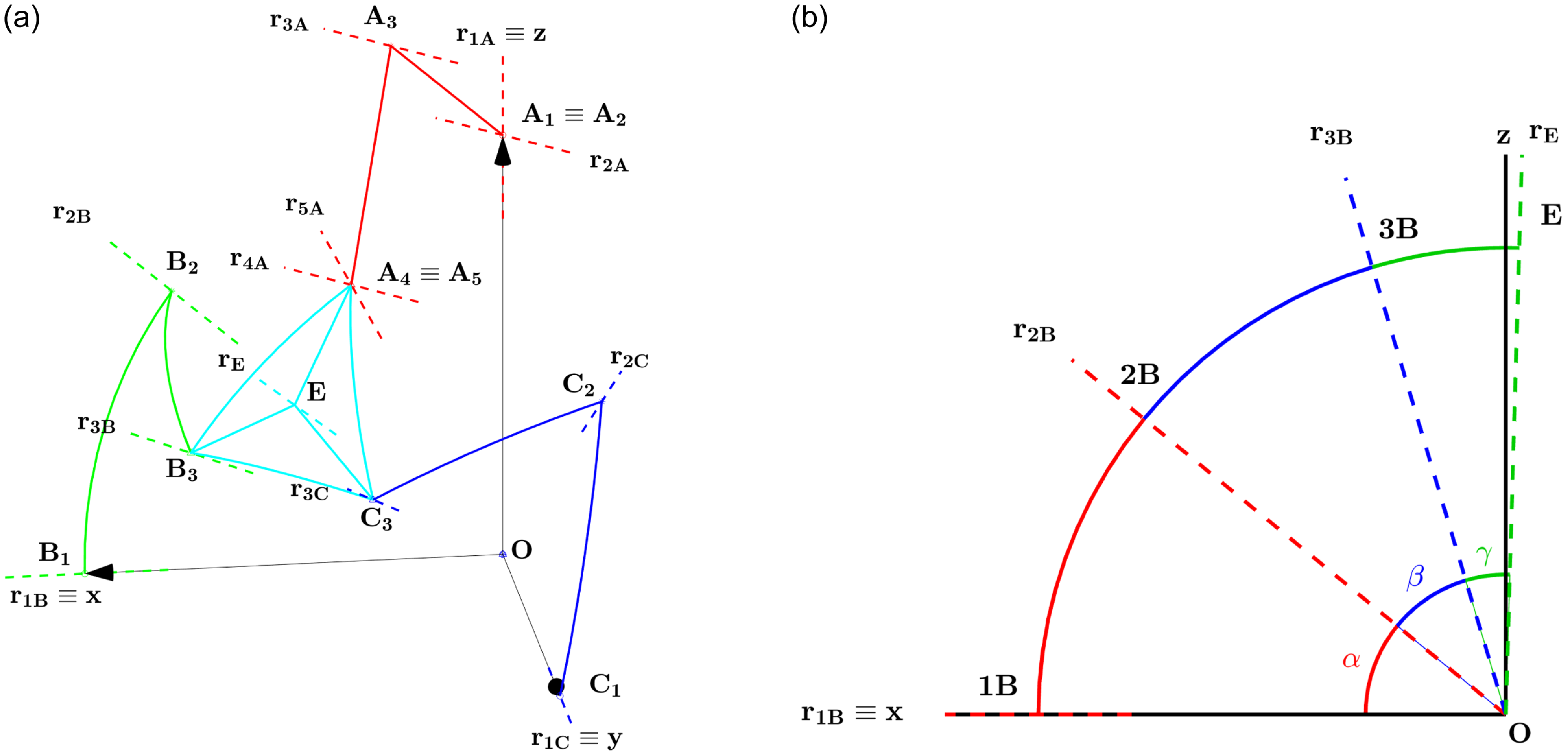
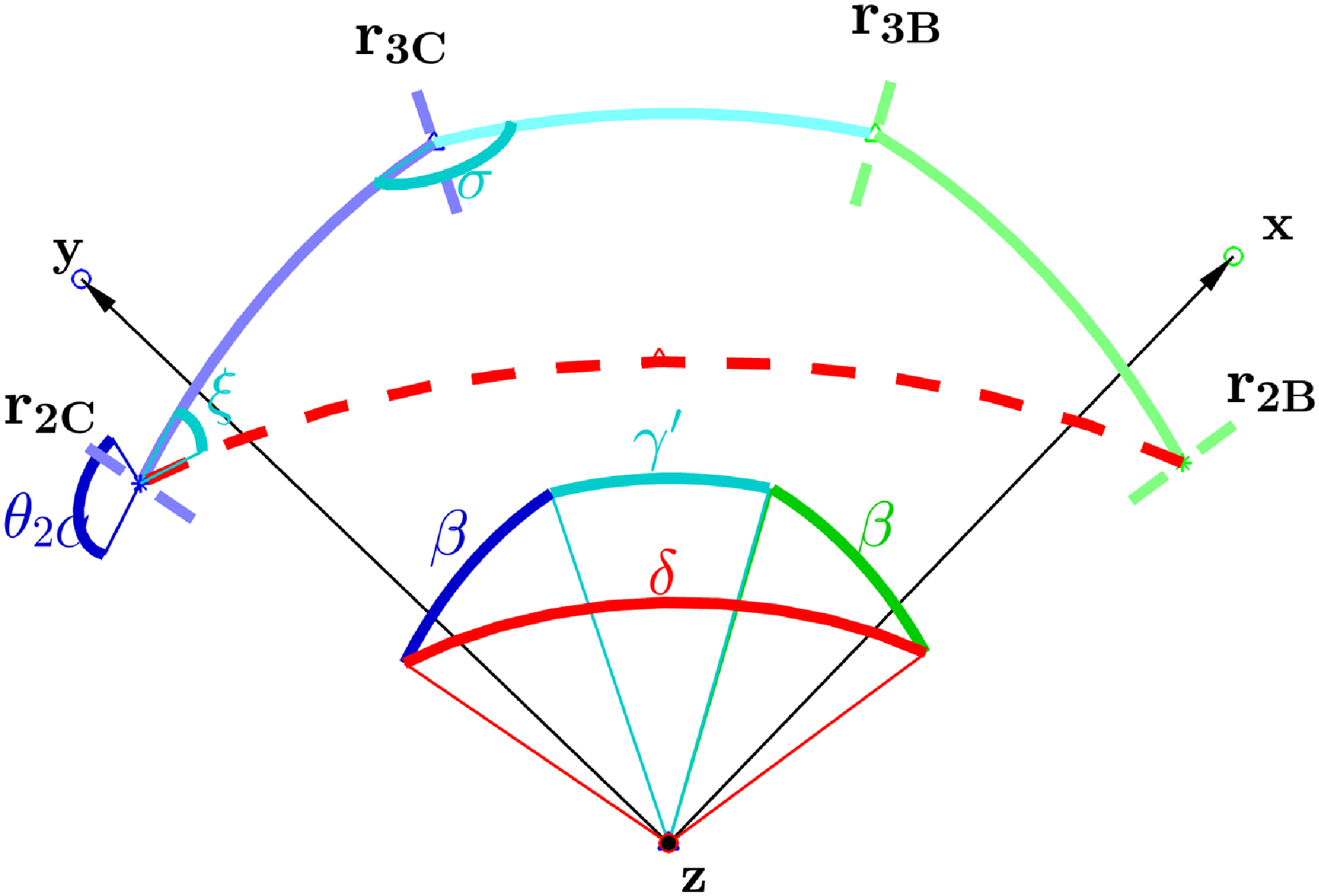
Schematized qSPM system in MATLAB environment, link nomenclature: legs A, B, C (red, green, blue), platform (cyan) (a). Geometrical angles definition of leg B on a common plane
 ${\boldsymbol{xz}}$
(b).

2. Kinematic Analysis
2.1. Main architecture assumptions
The proposed geometrical description of the qSPM, schematized in Figure 3a, derives from the following architecture assumptions:
-
M1) We define
 ${{\boldsymbol{r}}_{\boldsymbol{nK}}}|_{n=(1,\cdots, 5), K=(A,B,C)}$
the unitary vector referenced on the origin of the absolute RF
$({{\boldsymbol{O}},\hat{\boldsymbol{x}},\hat{\boldsymbol{y}},\hat{\boldsymbol{z}}})$
identifying the axis of revolution of a generic rotational joint
$K_n|_{n=(1,\cdots, 5), K=(A,B,C)}$
. We impose
${\boldsymbol{r}}_{\boldsymbol{1A}} \equiv {\hat{\boldsymbol{z}}}, {\boldsymbol{r}}_{\boldsymbol{1B}} \equiv {\hat{\boldsymbol{x}}}, {{\boldsymbol{r}}_{\boldsymbol{1C}}} \equiv {\hat{\boldsymbol{y}}}$
;
-
M2) For the superposition principle, universal joints of the URU leg can be divided in two rotative joints lying on perpendicular axes, namely
$A_1 \equiv A_2$
and
$A_4 \equiv A_5$
. Thus:
${\boldsymbol{r}}_{\boldsymbol{1A}} \perp {\boldsymbol{r}}_{\boldsymbol{2A}}$
and
${\boldsymbol{r}}_{\boldsymbol{4A}} \perp {\boldsymbol{r}}_{\boldsymbol{5A}}$
; -
M3) With such formulation, we define the constant geometrical angles
$(\alpha, \beta, \gamma )$
, respectively, identifying the proximal links’ and distal links’ angular span (i.e., respectively, angles
$K_1\hat{O}K_2|_{K=(B,C)}$
and
$K_2\hat{O}K_3|_{K=(B,C)}$
), and the angle
$E\hat{O}X|_{X=(A_4 \equiv A_5,B_3,C_3)}$
, as shown in Figure 3b; -
M4) Due to the architecture’s spherical geometry, and thus with minimal exceptions in the URU leg, links’ fundamental shapes only depend on geometrical angles of Assumption (M3). The overall description is thus scalable, having a quasi-spherical description;
-
M5) For the sake of brevity, we implicitly assume, unless stated otherwise, the formulation of vector
${{\boldsymbol{r}}_{\boldsymbol{nK}}}|_{n=(1,\cdots, 5), K=(A,B,C)} = R_{nK} \cdot {\hat{\boldsymbol{z}}}$
, being
$R_{nK}$
a suitable
$(3 \times 3)$
rotational matrix; -
M6) In order to be consistent with previous articles’ work [Reference Chaker, Mlika, Laribi, Romdhane and Zeghloul17–Reference Saafi, Laribi, Zeghloul and Arsicault19], the EE orientation
${{\boldsymbol{r}}_{\boldsymbol{E}}}$
is expressed in Euler
$zxz$
angles, as in (1);(1)In which:
\begin{equation} {\boldsymbol{r}}_{\boldsymbol{E}}(\psi, \theta, \phi ) = R_E(\psi, \theta, \phi ) {\hat{\boldsymbol{z}}} = R_z(\psi ) \cdot R_x(\theta ) \cdot R_z(\phi ) \end{equation}
$R_E$
and the triplet (
$\psi$
,
$\theta$
,
$\phi$
) the rotational matrix and the angles describing the
$zxz$
Euler description; inscriptions
$R_z (\!\cdot\!)$
and
$R_x (\!\cdot\!)$
rotation matrices around axes
${\hat{\boldsymbol{z}}}$
and
${\hat{\boldsymbol{x}}}$
.
-
M7) As described in Section 1, three motors are mounted on the proximal links and thus act on the active angles
$\theta _{1A}{\boldsymbol{r}}_{\boldsymbol{1A}}$
,
$\theta _{1B}{\boldsymbol{r}}_{\boldsymbol{1B}}$
, and
$\theta _{1C}{\boldsymbol{r}}_{\boldsymbol{1C}}$
.





2.2. Inverse kinematics model and working modes
Adopting the geometrical description as in Section 2.1, we can derive the inverse kinematics model (IKM) resolution as a trigonometric function of the active angles (2).
 \begin{align*} \;\;\;\qquad\qquad\qquad\qquad\qquad\qquad \left \{\begin{array}{c@{\quad}c@{\quad}c} A_1 \cdot \cos (\theta _{1A}) + A_2 \cdot \sin (\theta _{1A}) + A_3 &= 0 \qquad \qquad \qquad\qquad \qquad (2\textrm{a})\\[5pt] B_1 \cdot \cos (\theta _{1B}) + B_2 \cdot \sin (\theta _{1B}) + B_3 &= 0 \qquad \qquad \qquad \qquad\qquad (2\textrm{b})\\[5pt] C_1 \cdot \cos (\theta _{1C}) + C_2 \cdot \sin (\theta _{1C}) + C_3 &= 0 \qquad \qquad \qquad \qquad\qquad (2\textrm{c}) \end{array}\right .\nonumber \end{align*}
In which:
 $K_i|_{(K=A,B,C),i=(1,2,3)}$
are functions of constant and imposed angles
 $(\alpha, \beta, \gamma, \psi, \theta, \phi )$
and are reported in (34)(35)(36) in Appendix;
 $A_3=0$
due to the different structure of leg A.
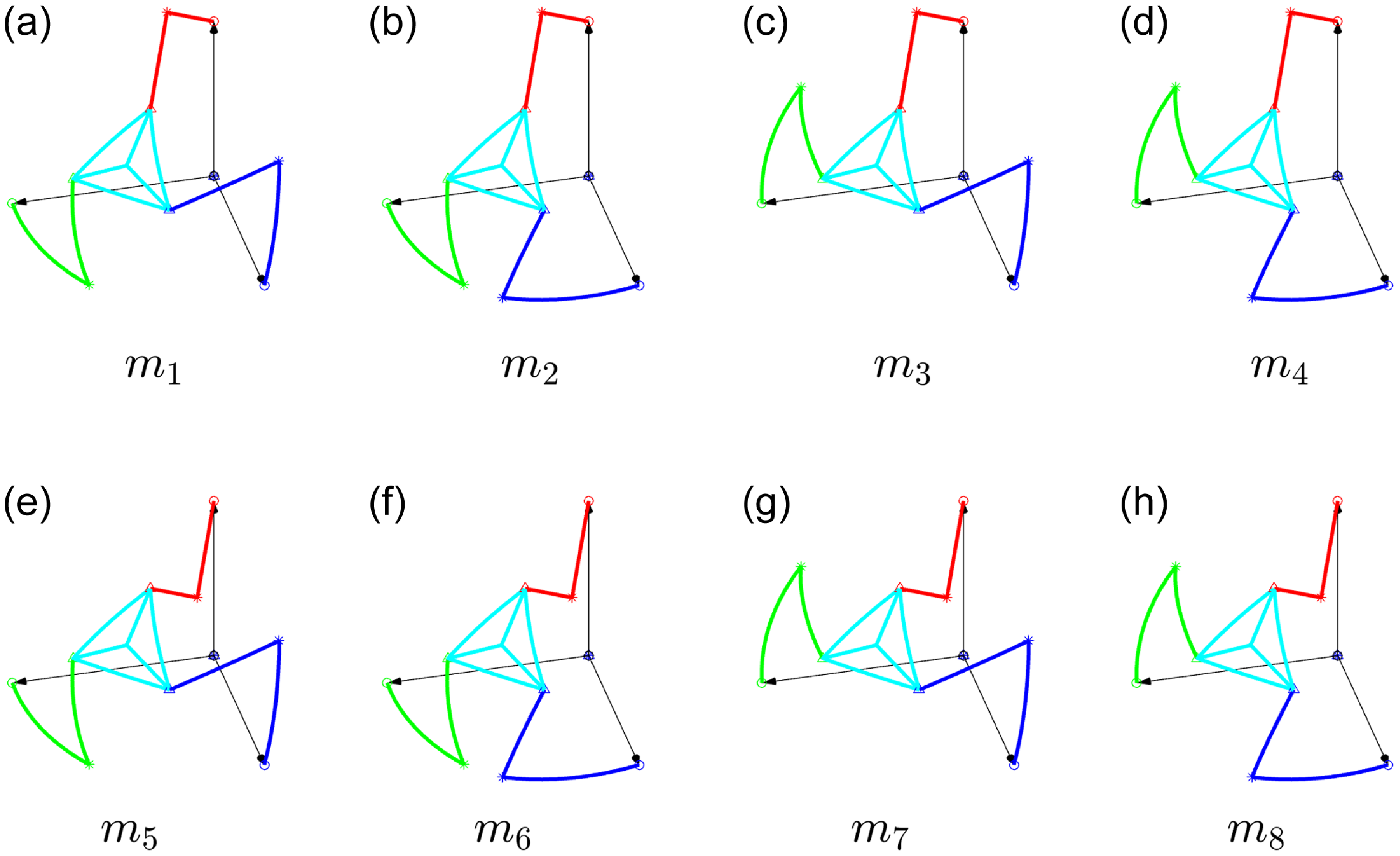
It can be demonstrated that the IKM admits eight solutions, or working modes
 $m_i|_{i=(1,\dots, 8)}$
, directly depending on the configuration of legs A, B, and C, as in Figure 4.
 \begin{equation} \begin{cases} \begin{alignedat}{3} \theta _{1A} =& \, atan2(\!-A_1,A_2)& \qquad (A_3 = 0), \, \, & m_i|_{i=(1,\dots, 8)} \\[5pt] \theta _{1B} =& \, atan2(y_{B1},x_{B1}) & \qquad & m_{1,5},m_{2,6} \\[5pt] & \, atan2(y_{B2},x_{B2}) & \quad & m_{3,7},m_{4,8} \\[5pt] \theta _{1C} =& \, atan2(y_{C1},x_{C1}) & \qquad & m_{1,5},m_{3,7} \\[5pt] & \, atan2(y_{C2},x_{C2}) & \qquad & m_{2,6},m_{4,8} \end{alignedat} \end{cases} \end{equation}
In which expressions of
 $x_{Ki} |_{K =(B,C), i = (1,2)}$
and
 $y_{Ki} |_{K =(B,C), i = (1,2)}$
are reported in (37) in Appendix.
2.3. Jacobian computation
The Jacobian matrix can be reconstructed by time deriving the geometric description of the three legs [Reference Saafi, Laribi, Zeghloul and Arsicault19]. The system can be reduced as in (4).
 \begin{equation} \boldsymbol{\omega } = J_p^{-1} J_s \dot{\boldsymbol{\Theta }} = J \dot{\boldsymbol{\Theta }} \end{equation}
In which:
 $\boldsymbol{\Theta } = [\theta _{1A},\theta _{1B},\theta _{1C}]^t$
is the joint vector;
 $\dot{\boldsymbol{\Theta }}$
and
 $\boldsymbol{\omega }$
are the angular speeds of the motors and the platform;
 $J_p$
(5a) and
 $J_s$
(5b) are the parallel and serial parts of the Jacobian.
 \begin{align*} \,\qquad\qquad\qquad\qquad\qquad \left \{ \begin{array}{l} J_p = \begin{bmatrix} ({\boldsymbol{r}}_{\boldsymbol{4A}} \times {\boldsymbol{r}}_{\boldsymbol{5A}})^t \\[5pt] ({\boldsymbol{r}}_{\boldsymbol{2B}} \times {\boldsymbol{r}}_{\boldsymbol{3B}})^t \\[5pt] ({\boldsymbol{r}}_{\boldsymbol{2C}} \times {\boldsymbol{r}}_{\boldsymbol{3C}})^t \\[5pt] \end{bmatrix}\qquad \qquad \qquad\qquad\qquad \, \qquad \qquad\qquad \qquad \qquad (5\textrm{a})\\[5pt] J_s = \begin{bmatrix} {\boldsymbol{r}}_{\boldsymbol{1A}} \cdot ({\boldsymbol{r}}_{\boldsymbol{4A}} \times {\boldsymbol{r}}_{\boldsymbol{5A}}) & 0 & 0\\[5pt] 0 & {\boldsymbol{r}}_{\boldsymbol{1B}} \cdot ({\boldsymbol{r}}_{\boldsymbol{2B}} \times {\boldsymbol{r}}_{\boldsymbol{3B}}) & 0\\[5pt] 0 & 0 & {\boldsymbol{r}}_{\boldsymbol{1C}} \cdot ({\boldsymbol{r}}_{\boldsymbol{2C}} \times {\boldsymbol{r}}_{\boldsymbol{3C}}) \end{bmatrix}\qquad \qquad \qquad (5\textrm{b}) \end{array}\right . \end{align*}
Note that
 $J$
implicitly depends on working modes
 $m_i|_{i=(1,\dots, 8)}$
due to the IKM structure.
Admitted working modes
 $m_i|_{i=(1,\dots, 8)}$
of the qSPM system.

2.4. Singularity definition
Singular positions can thus be achieved in three different ways:
-
• Serial singularity: happening if
$det(J_s)=0$
, that is, when factors of at least one triple product in expression (5b) are linearly dependent. This happens when the vectors lie on the same plane or at least two of them are parallel, that is, the legs are either fully retracted or fully extended, as shown in Figure 5a, and two solutions
$m_i|_{i=(1,\dots, 8)}$
coincide. Serial singularities tend to be outside of the operative workspace, defined in Section 3.1; -
• Parallel singularity: happening if
$det(J_p)=0$
, that is, when the matrix in (5a) is composed by linearly dependent vector entries, that is, when at least two of the planes containing
$(r_{3K},r_{2K})|_{K=(B,C)}$
or
$(r_{4A},r_{5A})$
are parallel, as shown in Figure 5b; -
• Structural singularity: happening when both determinants
$det(J_s)$
and
$det(J_p)$
are null.


Serial singularity example, obtained in
 $(\psi, \theta, \phi )=(179,54.7,0) (^{\circ })$
, in which leg B is fully extended and
 $m_{1}$
and
 $m_{3}$
coincide (a); parallel singularity example, obtained with
 $m_{3}$
in
 $(\psi, \theta, \phi )=(109.5,41.7,-40) (^{\circ })$
, in which planes described by vectors
 ${({\boldsymbol{r}}_{\boldsymbol{4A}},{\boldsymbol{r}}_{\boldsymbol{5A}})}$
(plane A, red) and
 ${({\boldsymbol{r}}_{\boldsymbol{2B}},{\boldsymbol{r}}_{\boldsymbol{3B}})}$
(plane B, green) are parallel (b).

2.5. Forward kinematics model
The forward kinematics model (FKM) of the architecture depends on the analysis of spherical four-bar loops presented in ref. [Reference Bai, Hansen and Angeles29]. In a similar way of what was done in ref. [Reference Saafi, Laribi and Zeghloul20], we can identify the
 $B_2B_3C_3C_2$
four-bar loop, expressed as in (6) (7).
 \begin{equation} {\boldsymbol{z}}^t \cdot R_x(\delta ) \cdot R_z(\pi - \xi ) \cdot R_x(\beta ) \cdot R_z(\pi - \sigma ) \cdot R_x(\gamma ') \cdot {\boldsymbol{z}} - {\boldsymbol{z}}^t \cdot \left (R_x(\beta )\right )^t \cdot {\boldsymbol{z}} = 0 \end{equation}
 \begin{equation} R_E = R_{2C} \cdot R_z(\theta _{2C}) \cdot R_x(\!-\beta ) \cdot R_z\left(\frac{5}{6} \cdot \pi +\sigma \right) \cdot R_x(\!-\gamma ) \cdot R_z(\!-\phi _E) \end{equation}
In which, as shown in Figure 6:
 $\xi$
and
 $\sigma$
are the input and output angles of the four-bar equations [Reference Bai, Hansen and Angeles29];
 $\delta$
is the angle between
 ${\boldsymbol{r}}_{\boldsymbol{2B}}$
and
 ${\boldsymbol{r}}_{\boldsymbol{2C}}$
, depending on the robot’s pose;
 $\gamma '$
is the constant angle between
 ${\boldsymbol{r}}_{\boldsymbol{3B}}$
and
 ${\boldsymbol{r}}_{\boldsymbol{3C}}$
;
 $R_{2C}$
derives from (M5);
 $\phi _E$
is a constant adjustment angle, as in Table II in Appendix.
Assuming as knowns the active angles
 $\theta _{1K}|_{K=(A,B,C)}$
,
 $\delta$
can be computed online. On the other hand,
 $\xi$
can be computed, with great computational gains, by adding an additional encoder measuring
 $\theta _{2C}$
. The Euler angles triplet (
 $\psi, \theta, \phi$
) can then be computed from (7) with reference to the Euler
 $zxz$
construction formulas.
Spherical four-bar loop used for the resolution of the FKM . Nomenclature from Figure 3a.

2.6. Haptic feedback
An haptic feedback system can then be built through the FKM, as in Section 2.5, providing the online computation of the Jacobian
 $J$
, and (8).
 \begin{equation} \boldsymbol{\tau } \stackrel{\text{def}}{=} \begin{bmatrix} \tau _{1A} \\[5pt] \tau _{1B} \\[5pt] \tau _{1C} \\[5pt] \end{bmatrix} = J^t \cdot {\boldsymbol{T}} + \boldsymbol\tau _{\boldsymbol{ctrl}} + \boldsymbol\tau _{\boldsymbol{comp}} \end{equation}
In which,
 $\tau _{1K}|_{K=(A,B,C)}$
are the active torques acting on the active angles
 $\theta _{1K}|_{K=(A,B,C)}$
;
 ${\boldsymbol{T}}$
are the operational torques acting on the slave robot’s tool and received by the master’s control algorithm;
 $\boldsymbol{\tau}_{\boldsymbol{ctrl}}$
are additional control torques that can be applied directly on the master device; and
 $\boldsymbol{\tau}_{\boldsymbol{comp}}$
are static compensation torques due to gravity acting on the qSPM mechanical elements.


3. Dominion analysis
3.1. Operative workspace definition
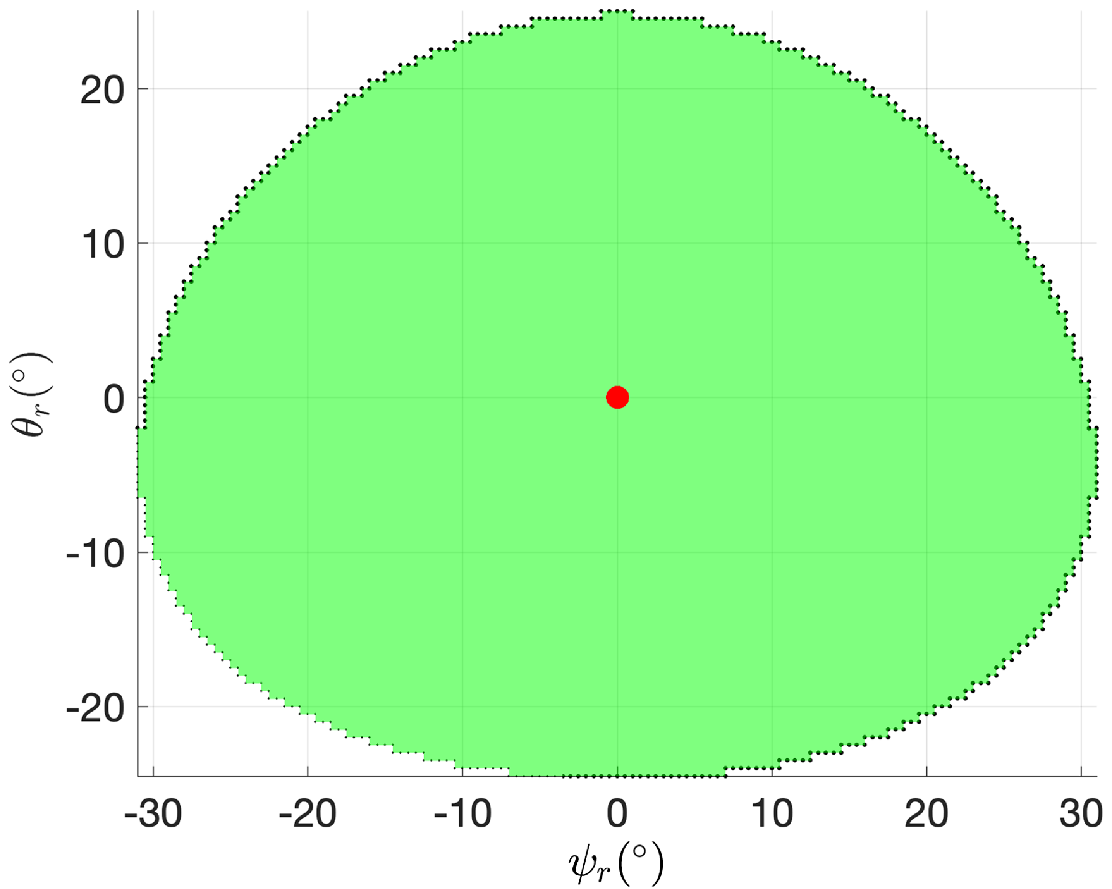
As mentioned in Section 1, the slave robot must operate on an RCM conic workspace built through a parametric cone demi-angle
 $\delta _C$
, as in Figure 2b. The operative workspace can be expressed in function of the Euler angles triplet (
 $\psi, \theta, \phi$
) as in (9):
 \begin{align*} \;\;\;\,\quad\qquad W_{op}= \left \{\begin{array}{l@{\quad}c} &\sin (\psi ) - \cos (\psi ) \cdot \sin (\theta ) + \cos (\theta ) \ge \sqrt{3} \cdot \cos (\delta /2)\\[-4pt] (\psi, \theta, \phi )\Bigg| \qquad & -50 ^{\circ } \leq \phi \leq 50 ^{\circ }\\[-4pt] & \delta = 50 ^{\circ } \end{array}\right \} \begin{array}{l@{\quad}c} &\qquad \qquad (9\textrm{a})\\[5pt] &\qquad \qquad (9\textrm{b})\\[5pt] &\qquad \qquad (9\textrm{c}) \end{array} \end{align*}
In which,
 $\delta _C$
is the cone demi-angle as in Figure 7; (9a) does not depend on the self-rotation angle
 $\phi$
due to conic symmetry of the workspace, and thus (9b) on
 $\phi$
is imposed; we assume, due to the geometric description presented in the previous paragraphs, a central workspace position
 $w_c$
as in (10).
 \begin{equation} \begin{aligned} {\boldsymbol{r}}_{\boldsymbol{wc}} =\frac{1}{\sqrt{3}} \begin{bmatrix} 1 \\[5pt] 1 \\[5pt] 1 \\[5pt] \end{bmatrix} & \quad & \Rightarrow &\quad & \begin{cases} \psi _{wc} &\thickapprox 135^{\circ }\\[5pt] \theta _{wc} &\thickapprox 54.7^{\circ }\\[5pt] \phi _{wc} &= 0^{\circ } \end{cases} \\[5pt] \end{aligned} \end{equation}
For the sake of brevity, we introduce the relative Euler angles triplet (
 $\psi _{r}, \theta _{r}, \phi _{r}$
) in (11). Workspace
 $W_{op}$
can be represented on the offset plane
 $\psi _r\theta _r$
independently from angle
 $\phi$
as in Figure 7.
 \begin{equation} \begin{cases} \psi _{r}(\psi ) = \psi - \psi _{wc}\\[5pt] \theta _{r}(\theta ) = \theta - \theta _{wc}\\[5pt] \phi _{r}(\phi ) = \phi - \phi _{wc} \end{cases} \end{equation}
We define
 $\delta _{E}$
as the angle between workspace center vector
 ${{\boldsymbol{r}}_{\boldsymbol{wc}}}$
(10), and the EE orientation vector
 ${\boldsymbol{r}}_{\boldsymbol{E}}(\psi _r,\theta _r,\phi _r)$
(1) (11), as in (12). Inside the workspace,
 $\delta _E \leq \delta _C$
due to (9).
 \begin{equation} \delta _E(\psi _r,\theta _r,\phi _r) = atan2({||{\boldsymbol{r}}_{\boldsymbol{wc}} \boldsymbol\times {\boldsymbol{r}}_{\boldsymbol{E}}||, {\boldsymbol{r}}_{\boldsymbol{wc}} \boldsymbol\cdot {\boldsymbol{r}}_{\boldsymbol{E}}}) \end{equation}
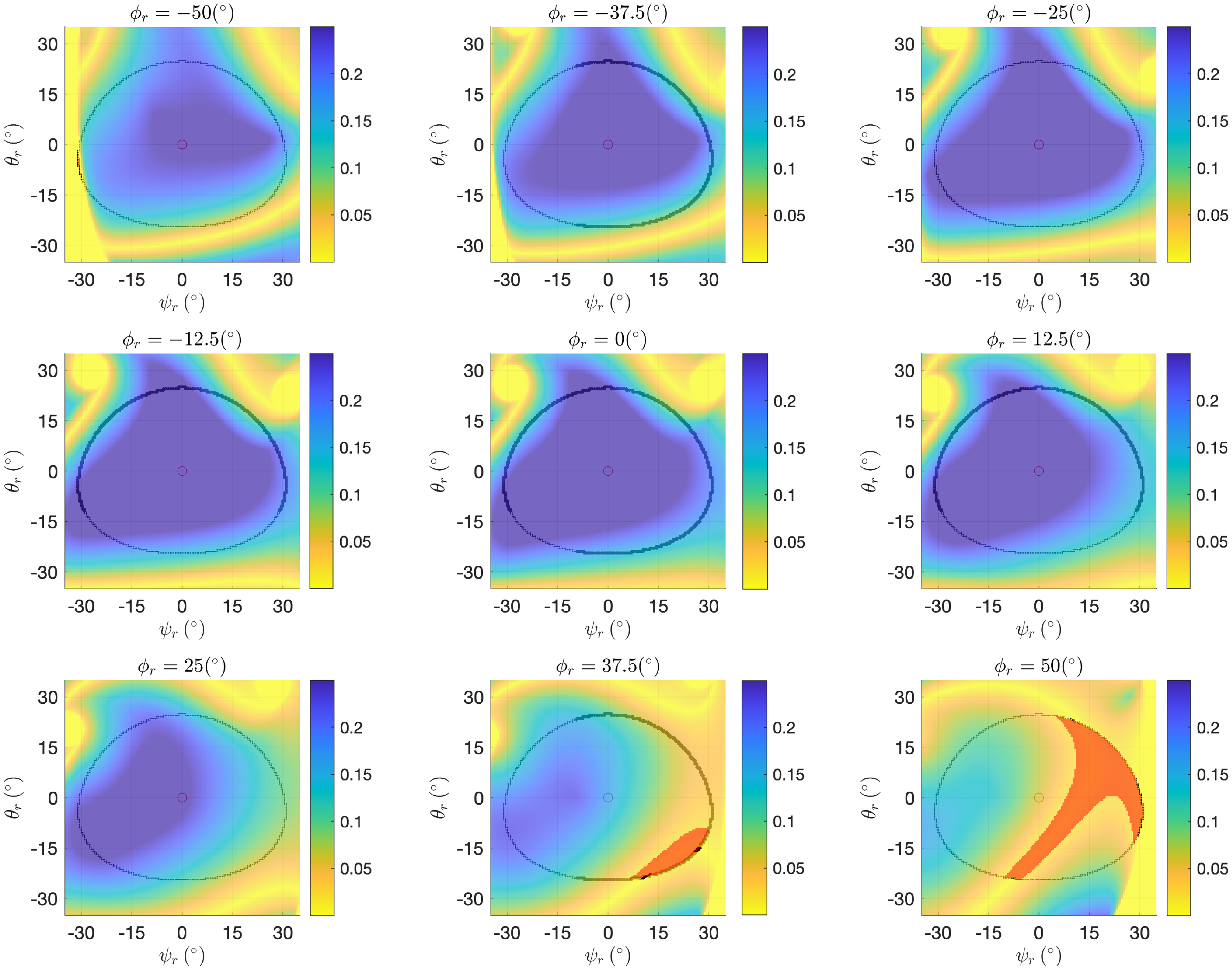
3.2. Dexterity maps
To enhance the analysis of singularities within the operative workspace, described in Section 3.1, for each working mode
 $m_i|_{i=(1,\dots, 8)}$
(3), we introduce the dexterity parameter
 $\eta (J)$
, defined as in (13).
 \begin{equation} \begin{aligned} \eta (J)=\frac{1}{||J|| \cdot ||J^{-1}||}, & \qquad & 0\lt \eta (J)\lt 1 \end{aligned} \end{equation}
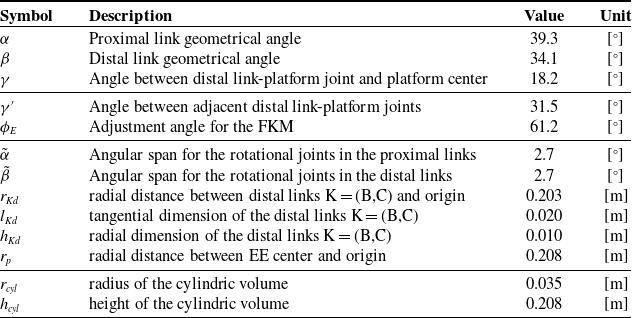
By imposing geometrical angles values as in Table II in Appendix, and a minimum dexterity threshold
 $\eta _{thr}=0.02$
, singularity areas
 $S_J$
can be defined by (14).
 \begin{equation} S_J = \{ (\psi _{r}, \theta _{r}, \phi _{r}) \mid \eta (J(\psi, \theta, \phi )) \lt \eta _{thr} = 0.02 \} \end{equation}


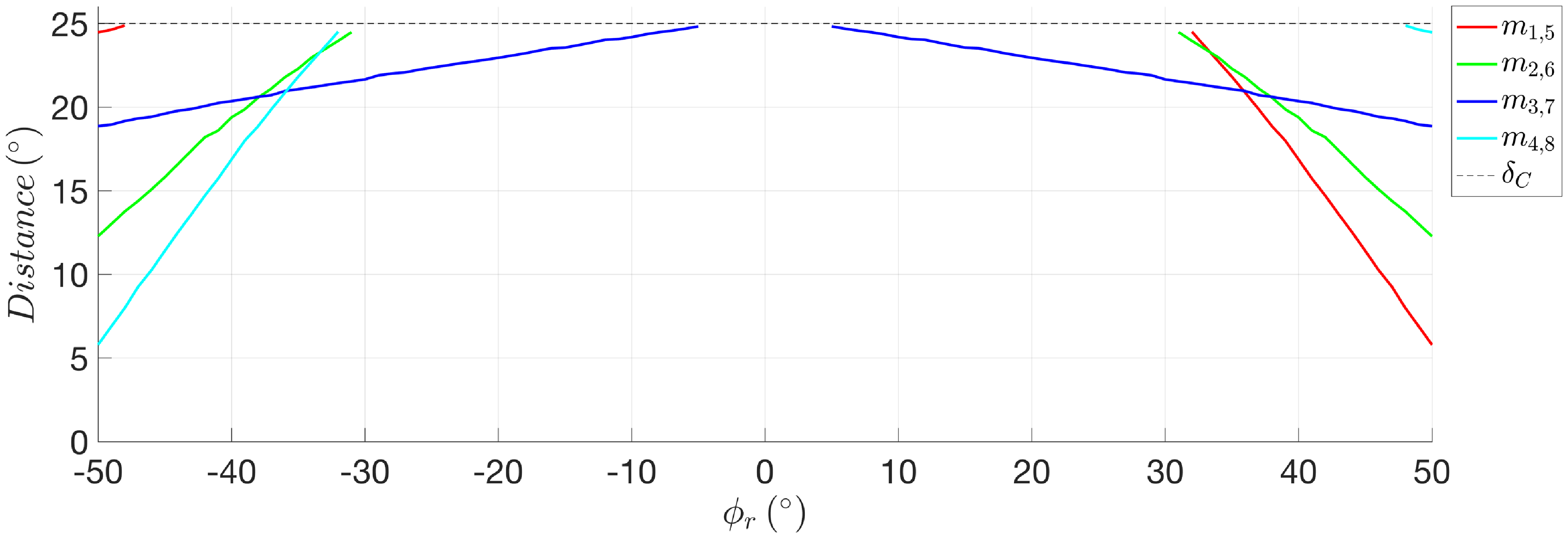
Performance index
 $\delta _{E,min,S_J}(\phi _r)$
of working modes
 $m_{i,i+4}|_{i=(1,\dots, 4)}$
(red, green, blue, and cyan). Black dashed line is
 $\delta _C$
(9).

Map results, depending on working modes
 $m_i|_{i=(1,\dots, 8)}$
, are shown inside the Euler
 $zxz$
space
 $(\psi _r, \theta _r,\phi _r)$
by varying discretely the Euler angle
 $\phi _r$
and analyzing planes
 $\psi _r\theta _r$
.
It can be demonstrated that, due to Assumptions (M1) and (M2) on the overall description of the architecture and (3), leg A’s configuration does not influence in any way the dexterity of the manipulator inside
 $W_{op}$
. Therefore, pairs of working modes
 $m_{i,i+4}|_{i=1,\dots, 4}$
produce the same dexterity maps. Figure 8 shows discrete results for
 $m_{1,5}$
and Figure 22 in Appendix for the other solutions.
3.3. Dexterity performance index and reachable workspace
As a mean to assess and compare working modes’ performances on dexterity, we introduce the performance index
 $\delta _{E,min,S_J}(\phi _r)$
. Said index corresponds to the partial minimization on planes
 $\psi _r\theta _r$
of all possible
 $\delta _E$
(12) corresponding to critical points
 $(\psi _r,\theta _r,\phi _r) \in S_J$
(14). Therefore, the index corresponds to the angular distance from workspace center to the nearest singularity point in the cartesian space. The index is expressed in (15) and is portrayed in Figure 9 for all working modes.
 \begin{equation} \delta _{E,min,S_J} (\phi _r) = \min _{\psi _r,\theta _r}{\delta _{E}(\psi _r,\theta _r,\phi _r)} \quad (\psi _r,\theta _r,\phi _r) \in S_J \end{equation}
Aspects
 $A_i|_{i=(1,\dots, 8)}$
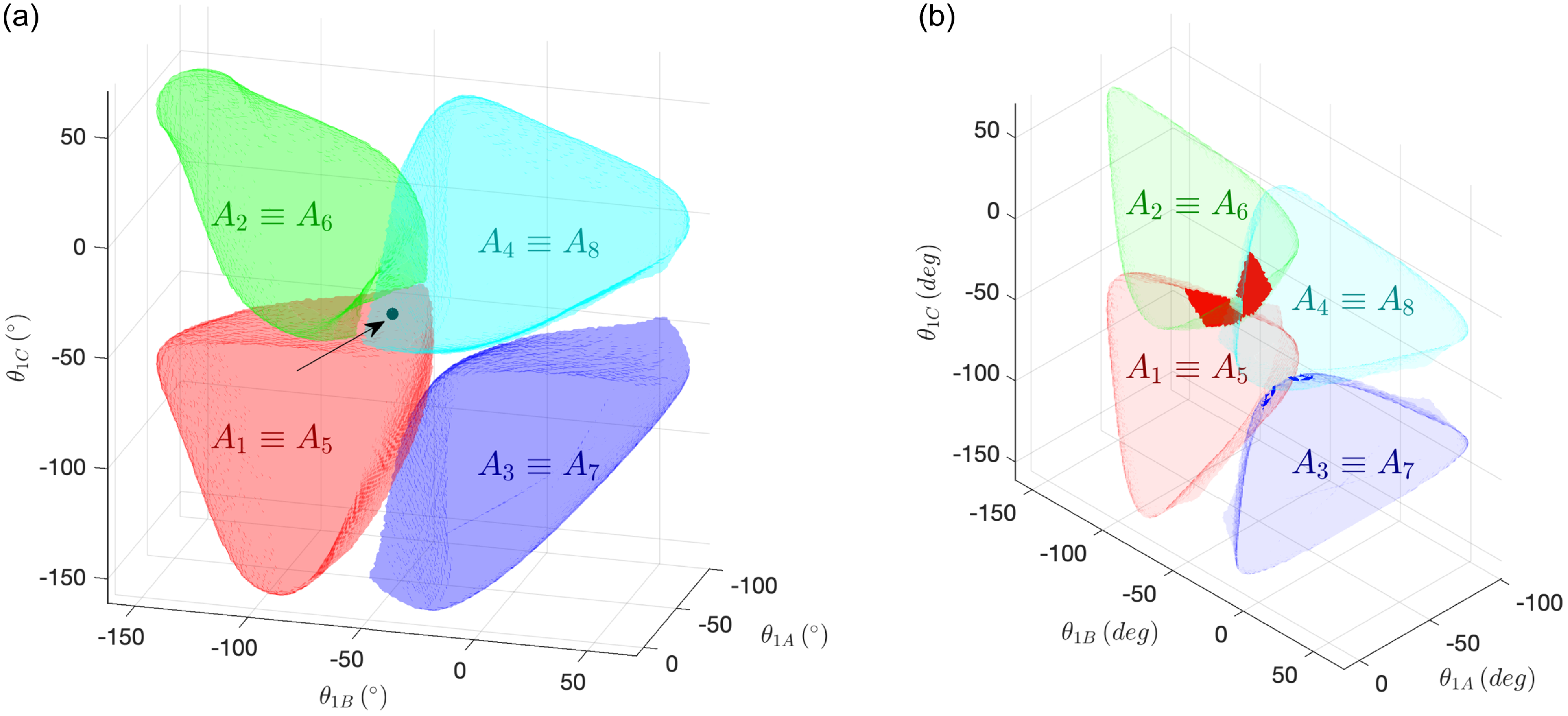
(red, green, blue, and cyan) defined in (17) inside the configuration space
 $(\theta _{1A}, \theta _{1B}, \theta _{1C})$
. Point-symmetry virtual center, to be discussed in Section 5.2, is a black dot highlighted by an arrow (a); Intersections (red) and tangential zones (blue) among aspects (b).

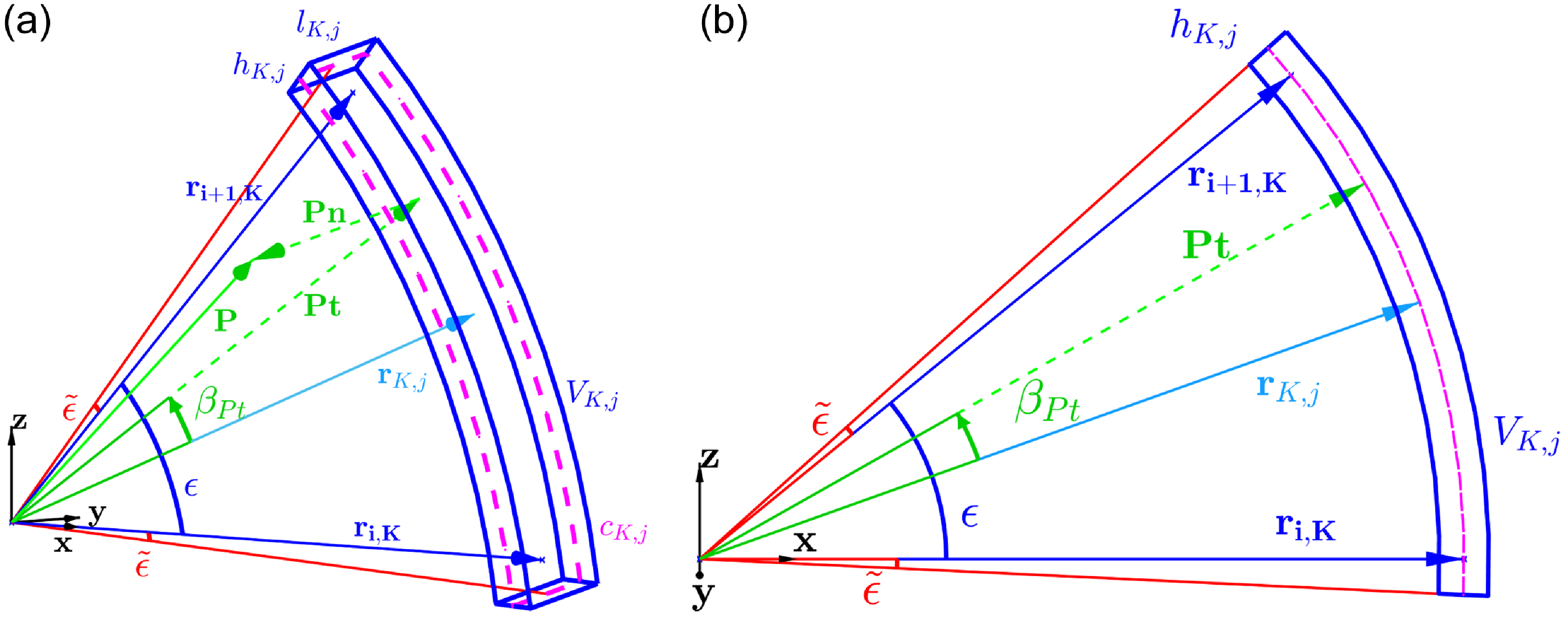
Parameters involved in the definition of a general link, with a generic point
 ${\boldsymbol{P}}$
, as in (20): generic view (a); View on plane
 $(r_{i,K},r_{i+1,k})$
(b).

Focusing, for example, on
 $m_{1,5}$
and thus Figure 8, note that, for
 $\phi _r = 50 ^{\circ }$
, there are parts of the workspace that are unreachable due to singularity crossings. The defined reachable workspace thus restricts according to the expression (16).
 \begin{equation} W_{reach} = \{ P=(\psi, \theta, \phi ) \in W_{op} \mid \exists s(w_c, P) \in C^0 \;:\; s(w_c, P) \cap S_J = \emptyset \} \end{equation}
In which,
 $s(w_c, P)$
is a random continuous path between point
 $P$
and the operative workspace center
 $w_c$
(10);
 $W_{reach}$
implicitly depends on to working modes
 $m_i|_{i=(1,\dots, 8)}$
through
 $S_J$
due to the Jacobian defined in Section 2.3.
3.4. Configuration space and aspects
Inside the configuration space, we define the Aspects
 $A_i|_{i=(1,\dots, 8)}$
as the images of the IKM function
 $f_{IKM}$
in the workspace
 $W_{reach}$
according to working modes
 $m_i|_{i=(1,\dots, 8)}$
as in (17) and Figure 10a.
 \begin{equation} A_i|_{i=(1,\dots, 8)} = \{ \Theta = (\theta _{1A}, \theta _{1B}, \theta _{1C}) \mid \exists (\psi, \theta, \phi ) \in W_{reach} \;:\; f_{IKM}(\psi, \theta, \phi ) = \Theta \} \end{equation}
As a direct product of the dexterity maps portrayed in Section 3.2, also Aspects
 $A_{i,i+4}|_{i=1,\dots, 4}$
are paired, providing the same results inside the configuration space.
4. Self-collision
4.1. Self-collision architecture assumptions
The self-collision phenomenon can involve either the legs, either, and possibly, the platform. To efficiently analyze the said phenomenon between legs, the following assumptions are needed:
-
A8) Every link in legs B and C can be defined, as in Figure 11, by the following parameters
$(K=(B,C), \, i=(1,2), \, j=(p,d)$
stands for “proximal” and “distal”):-
•
$\epsilon = (\alpha, \beta )$
is the geometrical angle of the link (M3); -
•
$\tilde{\epsilon }$
is the angular span which involves the non-lumped rotational joint; -
•
${{\boldsymbol{r}}_{\boldsymbol{i,K}}}$
and
${\boldsymbol{r}}_{{\boldsymbol{i}}\textbf{+1},{\boldsymbol{K}}}$
are the axes of its rotational joints; -
•
$r_{j,K}$
is the radial distance between the link’s geometrical center and the fixed RF origin; -
•
$l_{j,K}, h_{j,K}$
are, respectively, the tangential and radial dimensions of the link. -
•
$V_{d,K}|_{K=(A,B)}$
is the portion of space occupied by the link, function of the aforementioned parameters and the pose of the manipulator, that is, the active angles
$\Theta$
and
$m_i|_{i=(1,\dots, 8)}$
; -
•
$c_{d,K}|_{K=(A,B)}$
is the set of points defining the contour of the link lying in the spherical sector identified by
$r_{j,d}$
.
-
-
A9) Due to the involved rotational joint, the proximal and distal links of the same leg
$K$
do not lie within the same spherical sectors. Nevertheless, for simplicity, symmetry, system robustness, and manufacturing, it is assumed that
$r_{p,B} = r_{p,C}$
and
$r_{d,C} = r_{d,C}$
; -
A10) It is assumed that, in the qSPM, self-collision between legs happens only between distal links. Proximal links can collide only with working modes
$m_{2,6}$
and values of
$\alpha +\tilde{\alpha } \geq 45 ^{\circ }$
. Having imposed, as in Table II in Appendix,
$\alpha +\tilde{\alpha } \approx 42 ^{\circ }$
, from now on we will focus only on distal links.


In addition with the legs’ self-collision phenomenon, in prospect of a future axial displacement actuation along
 ${\boldsymbol{r}}_{\boldsymbol{E}}$
, this article also analyzes the self-collision phenomenon between the legs and a cylindric volume having as axis
 ${\boldsymbol{r}}_{\boldsymbol{E}}$
, as in Figure 12a. Additional assumptions are then required:
-
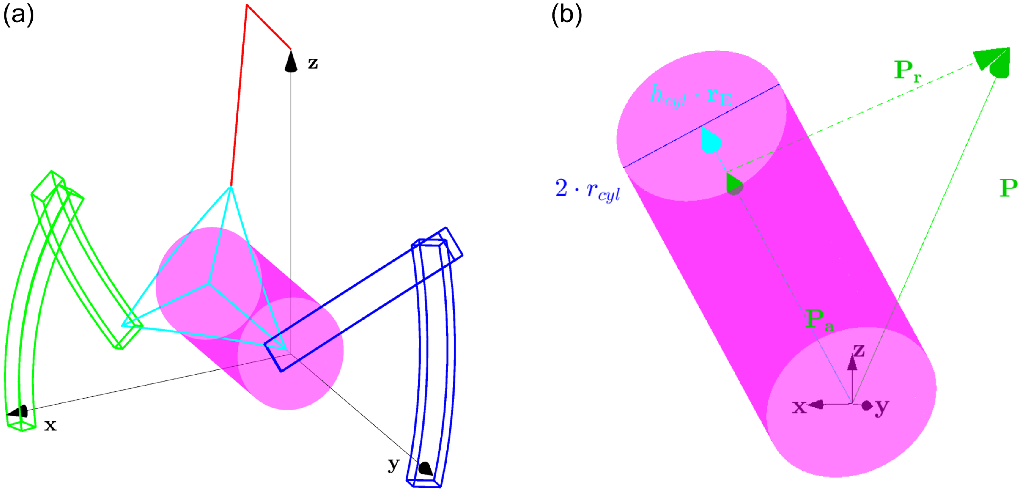
A11) Said cylinder can be defined with the following parameters, as in Figure 12b:
-
•
$r_{cyl}$
and
$h_{cyl}$
are the radius and the height of the cylinder, reported in Table II in Appendix; -
•
$V_{cyl}$
is the portion of space occupied by the cylinder;
With such formulation, the cylinder develops from point
${\boldsymbol{O}}$
(origin of the absolute RF) to point
$h_{cyl}{\boldsymbol{r}}_{\boldsymbol{E}}$
; -
-
A12) It can be demonstrated that the cylindric volume can collide only with the distal links inside the reachable workspace enriched with the collision phenomenon, to be presented in (25). Therefore, for the sake of brevity, collision between said volume and the proximal links is not analyzed.


Due to the superposition principle, the self-collision problem can then be divided in three subproblems, which can be analyzed separately: the collisions between distal links
 $V_{d,B}$
and
 $V_{d,C}$
; between distal link
 $V_{d,B}$
and cylinder
 $V_{cyl}$
; between distal link
 $V_{d,C}$
and cylinder
 $V_{cyl}$
.
Parameters involved in the definition of a general cylinder, with a generic point
 ${\boldsymbol{P}}$
, as in (20): contextual view (in
 $m_3$
,
 $(\psi _r,\theta _r,\phi _r)=(0,0,0)$
) (a); detailed view (b).

4.2. Self-collision description
4.2.1. Self-collision between distal links
With the premises made in the first part of Section 4.1, we can note that collision between distal links, labeled for brevity as
 $C1$
, happens with the expression (18):
 \begin{equation} C1 \iff \exists {\boldsymbol{P}} \;:\; {\boldsymbol{P}} \in V_{d,B} \cap V_{d,C} \end{equation}
From the perspective of logical computation, this condition can be reduced, with great computational gains, in the expression (19):
 \begin{equation} C1 \iff \exists {\boldsymbol{P}}_{\textbf{1}} \;:\; ({\boldsymbol{P}}_{\textbf{1}} \in c_{d,B} \cap V_{d,C}) \lor \exists {\boldsymbol{P}}_{\textbf{2}} \;:\; ({\boldsymbol{P}}_{\textbf{2}} \in c_{d,C} \cap V_{d,B}) \end{equation}
The problem then translates in identifying the logical conditions for which a general point
 ${\boldsymbol{P}}$
is inside the dominion
 $V_{d,K}$
(20) and apply said conditions to a discrete number of points in the contour
 $c_{d,K}$
of the other link.
 \begin{equation} {\boldsymbol{P}} \in V_{d,K} \iff \begin{cases} \begin{aligned} |\beta _{Pt}| &\leq \frac{\beta }{2} + \tilde{\beta }\\[5pt] r_{d,K} - \frac{h_{d,K}}{2} &\leq |{\boldsymbol{P}}_{\boldsymbol{t}}| \leq r_{d,K} + \frac{h_{d,K}}{2} \\[5pt] |{\boldsymbol{P}}_{\boldsymbol{n}}| &\leq \frac{l_{d,K}}{2} \\[5pt] \end{aligned} \end{cases} \end{equation}
In which:
 ${\boldsymbol{P}} = {\boldsymbol{P}}_{\boldsymbol{t}} + {\boldsymbol{P}}_{\boldsymbol{n}}$
, being
 ${\boldsymbol{P}}_{\boldsymbol{t}}$
and
 ${\boldsymbol{P}}_{\boldsymbol{n}}$
the tangential and normal projection vectors of
 ${\boldsymbol{P}}$
on the plane identified by vectors
 ${{\boldsymbol{r}}_{\boldsymbol{2K}},{\boldsymbol{r}}_{\boldsymbol{3K}}}$
;
 $\beta _{Pt}$
is the angle between
 $r_{d,K}{\hat{\boldsymbol{r}}}$
and
 ${\boldsymbol{P}}_{\boldsymbol{t}}$
, as portrayed in Figure 11.
4.2.2. Self-collision between distal links and cylinder
With the premises made in the second part of Section 4.1, we can note that collisions between the cylindric volume and the distal links, labeled for brevity as
 $C2$
and
 $C3$
, happens only when (21) is satisfied.
 \begin{equation} C2 \iff \exists {\boldsymbol{P}} \;:\; {\boldsymbol{P}} \in V_{d,B} \cap V_{cyl}, \quad C3 \iff \exists {\boldsymbol{P}} \;:\; {\boldsymbol{P}} \in V_{d,C} \cap V_{cyl} \end{equation}
From the computational point of view, as previously done with
 $C1$
, the problem can be reduced by identifying the logical conditions for which a general point
 ${\boldsymbol{P}}$
is inside the dominion
 $V_{cyl}$
(22) and apply them to a discrete number of points of the contours
 $c_{d,B}$
and
 $c_{d,C}$
, respectively, identifying
 $C2$
and
 $C3$
.
 \begin{equation} {\boldsymbol{P}} \in V_{d,K} \iff \begin{cases} \begin{aligned} |{\boldsymbol{P}}_{\boldsymbol{r}}| \leq r_{cyl} \\[5pt] |{\boldsymbol{P}}_{\boldsymbol{a}}| \leq h_{cyl} \\[5pt] \end{aligned} \end{cases} \overset{h_{cyl} \equiv r_p}{\implies } |{\boldsymbol{P}}_{\boldsymbol{r}}| \leq r_{cyl} \end{equation}
In which:
 ${\boldsymbol{P}} = {\boldsymbol{P}}_{\boldsymbol{r}} + {\boldsymbol{P}}_{\boldsymbol{a}}$
, being
 ${\boldsymbol{P}}_{\boldsymbol{r}}$
and
 ${\boldsymbol{P}}_{\boldsymbol{a}}$
the radial and axial projection vectors of
 ${\boldsymbol{P}}$
on axis
 ${\boldsymbol{r}}_{\boldsymbol{E}}$
, as in Figure 12b;
 $r_P$
is the actual distance between the EE center and the origin, reported in Table II in Appendix. Note that, imposing
 $h_{cyl} \equiv r_P$
, the condition on
 ${\boldsymbol{P}}_{\boldsymbol{a}}$
is always satisfied for every point inside
 $V_{d,K}|_{K=(B,C)}$
, and therefore can be simplified.
Experimental evaluation of this kind of collision is presented in Section 5.5.
4.3. Reachable workspace, dexterity maps, and performance index with collision
We can then enrich the reachable workspace introduced in (16) and the dexterity maps of Section 3.2 with the self-collision phenomenon between the two distal links and the cylindric volume. The resulting collision dominion
 $C_V$
, the reduced collision dominion
 $\tilde{C}_V$
, considering only
 $C1$
, and the reachable workspace
 $W_{reach,c}$
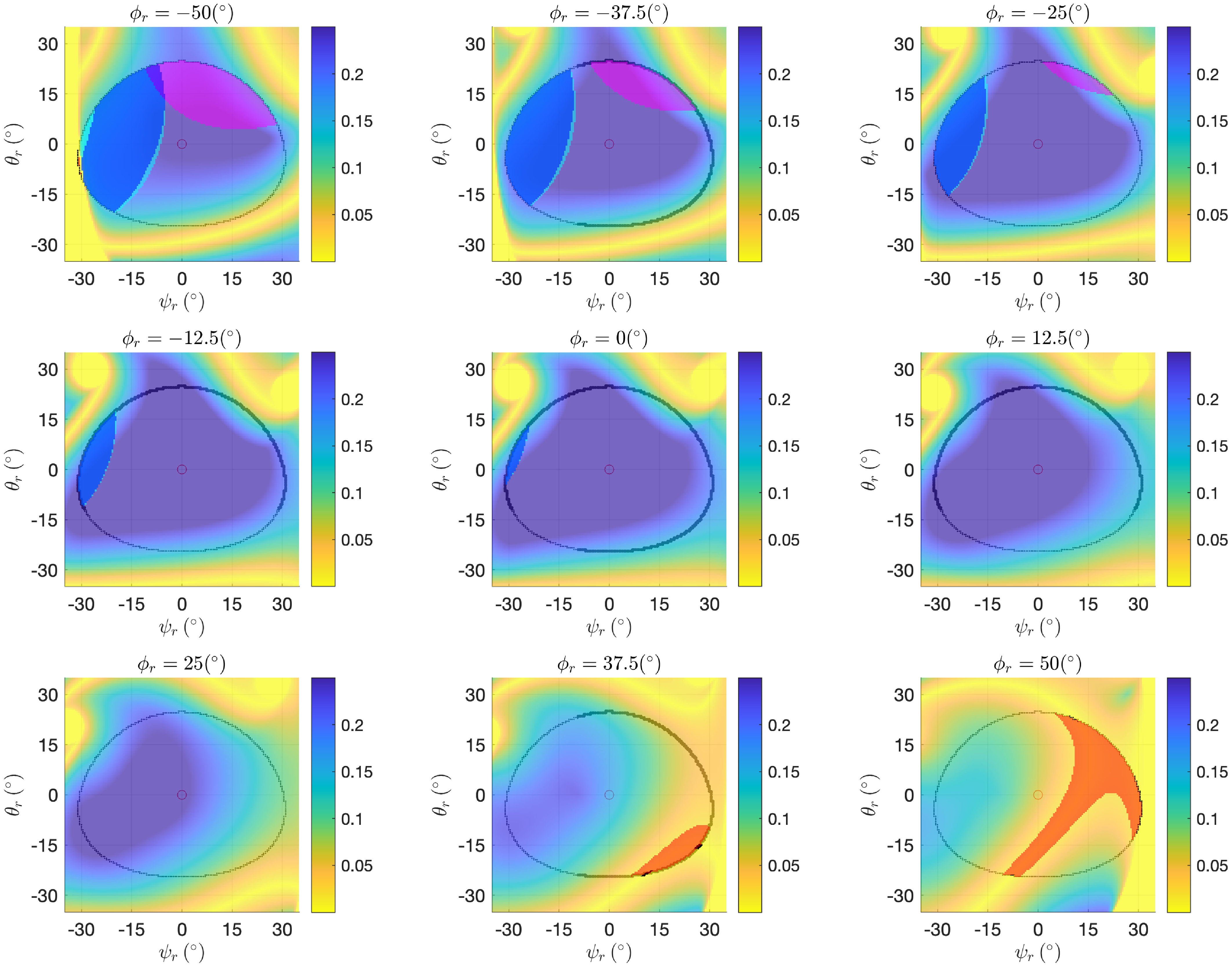
are described by (23) and (25), and discretely shown in Figure 13.
 \begin{equation*} \;\;\qquad\qquad\qquad\qquad\qquad\qquad C_V = \left \{\begin{array}{l@{\quad}l} & C1: \, V_{d,B} \cap V_{d,C} \neq \emptyset \\[-4pt] (\psi _{r}, \theta _{r}, \phi _{r})\Bigg| & C2: \, V_{d,B} \cap V_{cyl} \neq \emptyset \\[-4pt] & C3: \, V_{d,C} \cap V_{cyl} \neq \emptyset \end{array} \right \} \begin{array}{l@{\quad}c} &\qquad\qquad\qquad \qquad (23\textrm{a})\\[5pt] &\qquad\qquad \qquad\qquad (23\textrm{b})\\[5pt] &\qquad \qquad\qquad\qquad (23\textrm{c}) \end{array} \end{equation*}
 \begin{equation} \tilde{C}_V = \{ (\psi _{r}, \theta _{r}, \phi _{r}) \mid C1: \, V_{d,B} \cap V_{d,C} \neq \emptyset \} \end{equation}
 \begin{equation} W_{reach,c} = \{ P \in W_{op} \mid \exists s(w_c, P) \in C^0 \;:\; s(w_c, P) \cap (S_J \cup C_V) = \emptyset \} \end{equation}
Dexterity map in the Euler angles space for
 $m_{1,5}$
. Planes
 $\psi _{r}\theta _{r}$
with a discrete-step of
 $\phi _{r,step} =12.5^{\circ }$
. Relative angles defined in (11). Colored areas correspond, respectively, to singularity areas
 $S_J$
(red) (14) and collision areas
 $C_V$
(blue:
 $C1$
, cyan:
 $C2$
, magenta:
 $C3$
as in Section 4.2) (23) inside the operative workspace
 $W_{op}$
(9).

In a similar manner of Section 3.3, we can define two other performance indices, considering
 $C_V$
(23) and
 $\tilde{C}_V$
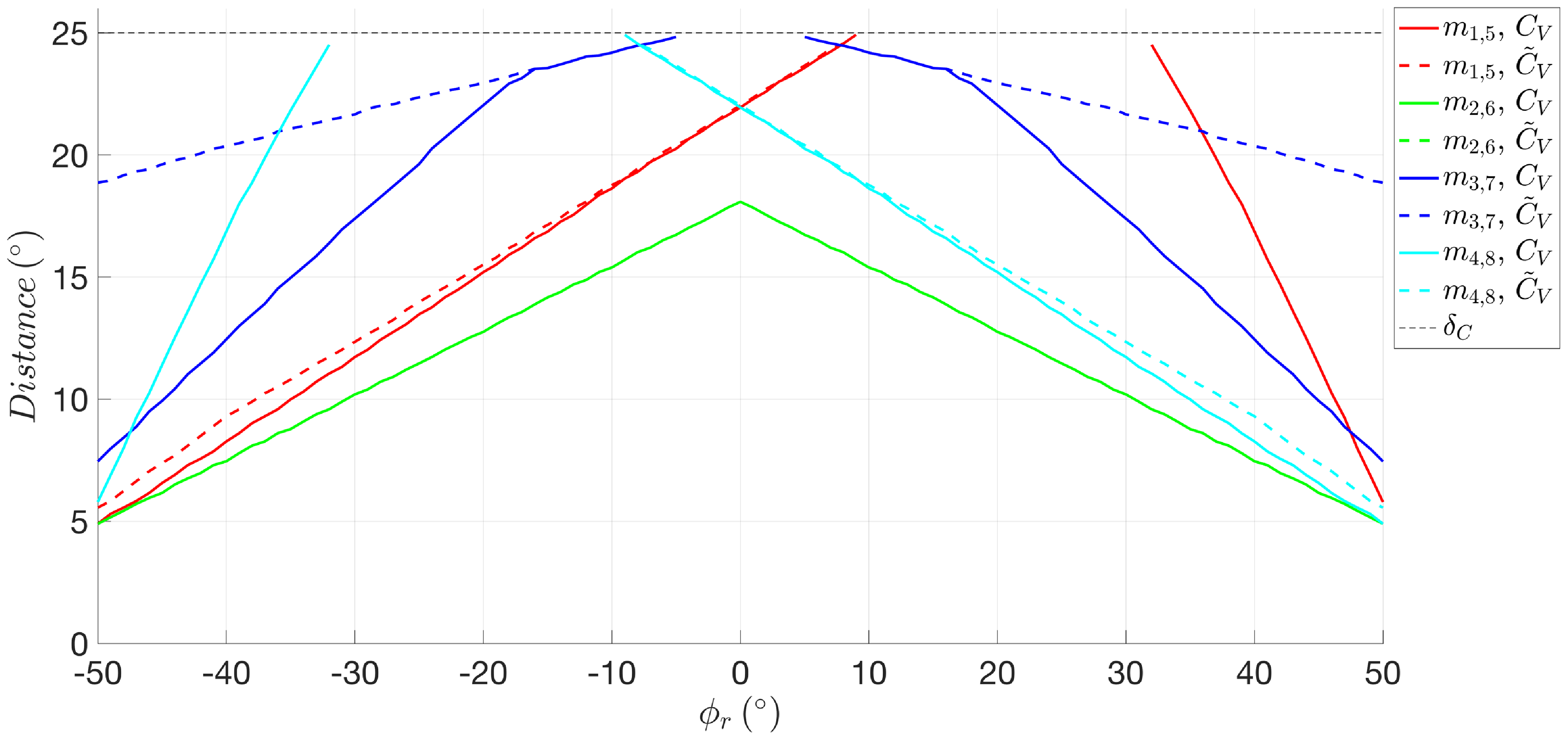
(24), as in (26) and (27). Figure 14 shows the two indices for all possible working modes
 $m_i|_{i=(1,\dots, 8)}$
.
 \begin{equation} \delta _{E,min,C_V} (\phi _r) = \min _{\psi _r,\theta _r}{\delta _{E}(\psi _r,\theta _r,\phi _r)} \quad (\psi _r,\theta _r,\phi _r) \in C_V \end{equation}
 \begin{equation} \delta _{E,min,\tilde{C}_V} (\phi _r) = \min _{\psi _r,\theta _r}{\delta _{E}(\psi _r,\theta _r,\phi _r)} \quad (\psi _r,\theta _r,\phi _r) \in \tilde{C}_V \end{equation}
Performance indices
 $\delta _{E,min,C_V}(\phi _r)$
(continuous lines) and
 $\delta _{E,min,\tilde{C}_V}(\phi _r)$
(dashed lines) of working modes
 $m_{i,i+4}|_{i=(1,\dots, 4)}$
(red, green, blue, and cyan) with collision. Black dashed line is
 $\delta _C$
(9).

4.4. Aspects enriched with collision
The knowledge of the workspace
 $W_{reach,c}$
(25), enriched with the collision phenomenon, allows for the updated definition of the Aspects
 $A_i|_{i=(1,\dots, 8),c}$
according to working modes
 $m_i|_{i=(1,\dots, 8)}$
inside the configuration space (28).
 \begin{equation} \begin{aligned} A_i|_{i=(1,\dots, 8),c} = \{\Theta = (\theta _{1A}, \theta _{1B}, \theta _{1C}) \mid \exists (\psi, \theta, \phi ) \in W_{reach,c} \;:\; f_{IKM}(\psi, \theta, \phi ) = \Theta \} \end{aligned} \end{equation}
5. Discussion
5.1. Observations on dexterity maps
Focusing on Sections 3.2 and 3.3, the following observations on
 $W_{reach}$
(16), the dexterity maps, in Figures 8 and 22, and the performance index
 $\delta _{E,min,S_J}$
(15) in Figure 9, can be made:
-
D1) As expected by the geometrical structure of the system, and by the symmetry of Assumption (M3), making both the proximal and the distal links equal with each other, working modes
$m_{2,6}$
and
$m_{3,7}$
are self-symmetric with respect to the workspace center, while
$m_{1,5}$
and
$m_{4,8}$
are symmetric with each other. The symmetry can be observed from both the dexterity maps and the euclidean distance plot; -
D2) Even if working modes
$m_{1,5}$
and
$m_{4,8}$
share the lowest
$\delta _{E,min,S_J}$
, working modes
$m_{3,7}$
can be considered, with only these premises, the worst modes, having singularity areas
$S_J$
even for
$|\phi _r| \leq 31 ^{\circ }$
; -
D3) Given Observation (D2), working modes
$m_{2,6}$
are the best configuration for the device’s dexterity.


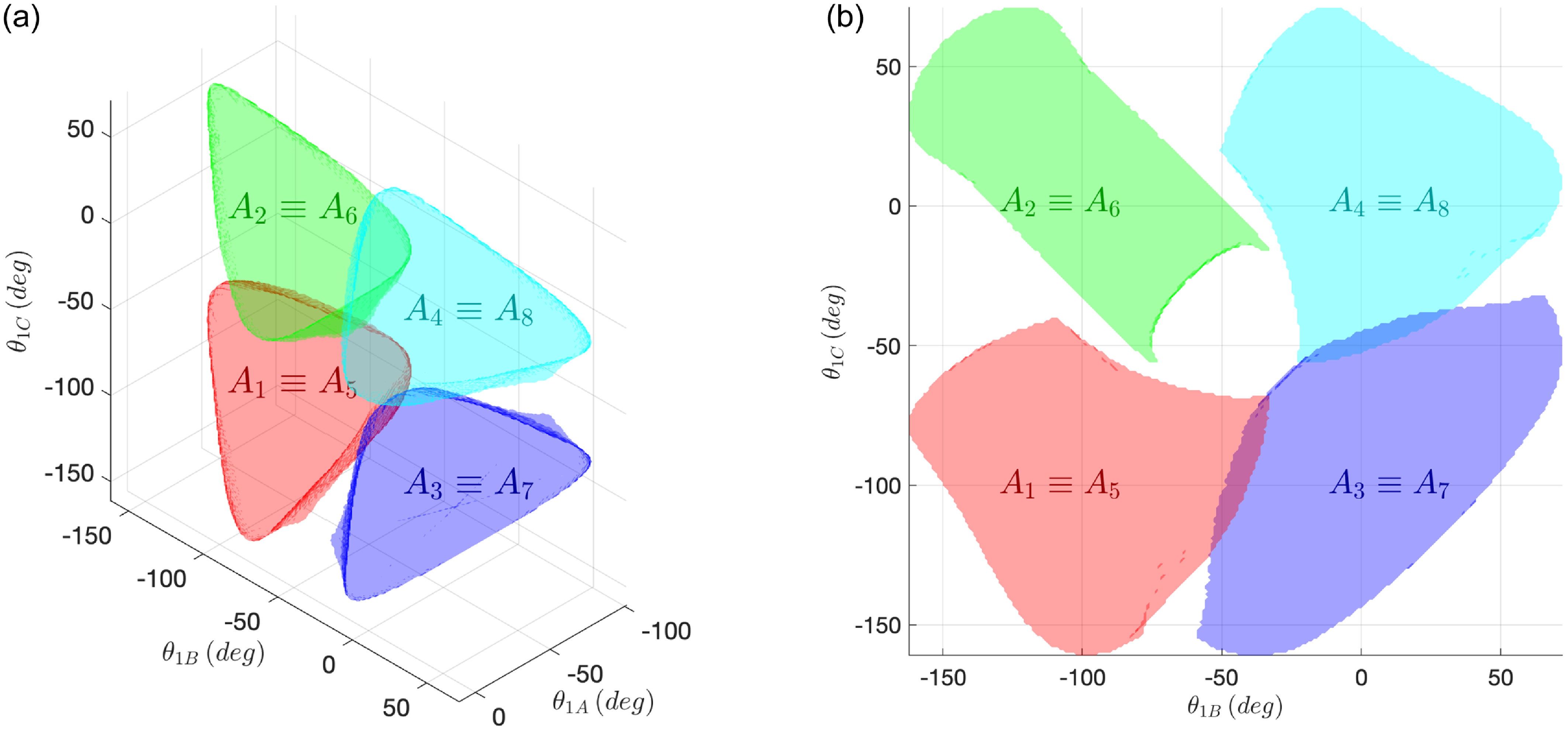
Aspects
 $A_i|_{i=(1,\dots, 8),c}$
(red, green, blue, and cyan) (28), enriched with the collision phenomenon, inside the configuration space
 $(\theta _{1A}, \theta _{1B}, \theta _{1C})$
(a)(b).

5.2. Observations on aspects
Focusing on Section 3.4, the following observations on
 $A_i|_{i=(1,\dots, 8)}$
(17) can be made:
-
E1) Due to their symmetric structure of the system, explained in Observation D1,
$A_{1,5}$
and
$A_{4,8}$
are point-symmetric toward a virtual center, highlighted by a black dot and an arrow in Figure 10a; -
E2) As portrayed by Figure 10b,
$A_{3,7}$
intersect both
$A_{1,5}$
and
$A_{4,8}$
in two tangential surface areas, that is, the singularity zones in which one 3-RRR leg is extended; -
E3) Couples
$(A_{1,5},A_{4,8})$
and
$(A_{2,6},A_{4,8})$
do not intersect nor touch each other. This is because it is not physically feasible to directly transition between the mentioned couple dominions, as the two 3-RRR legs can only extend one at a time; -
E4) Aspects
$A_{2,6}$
intersect both
$A_{1,5}$
and
$A_{4,8}$
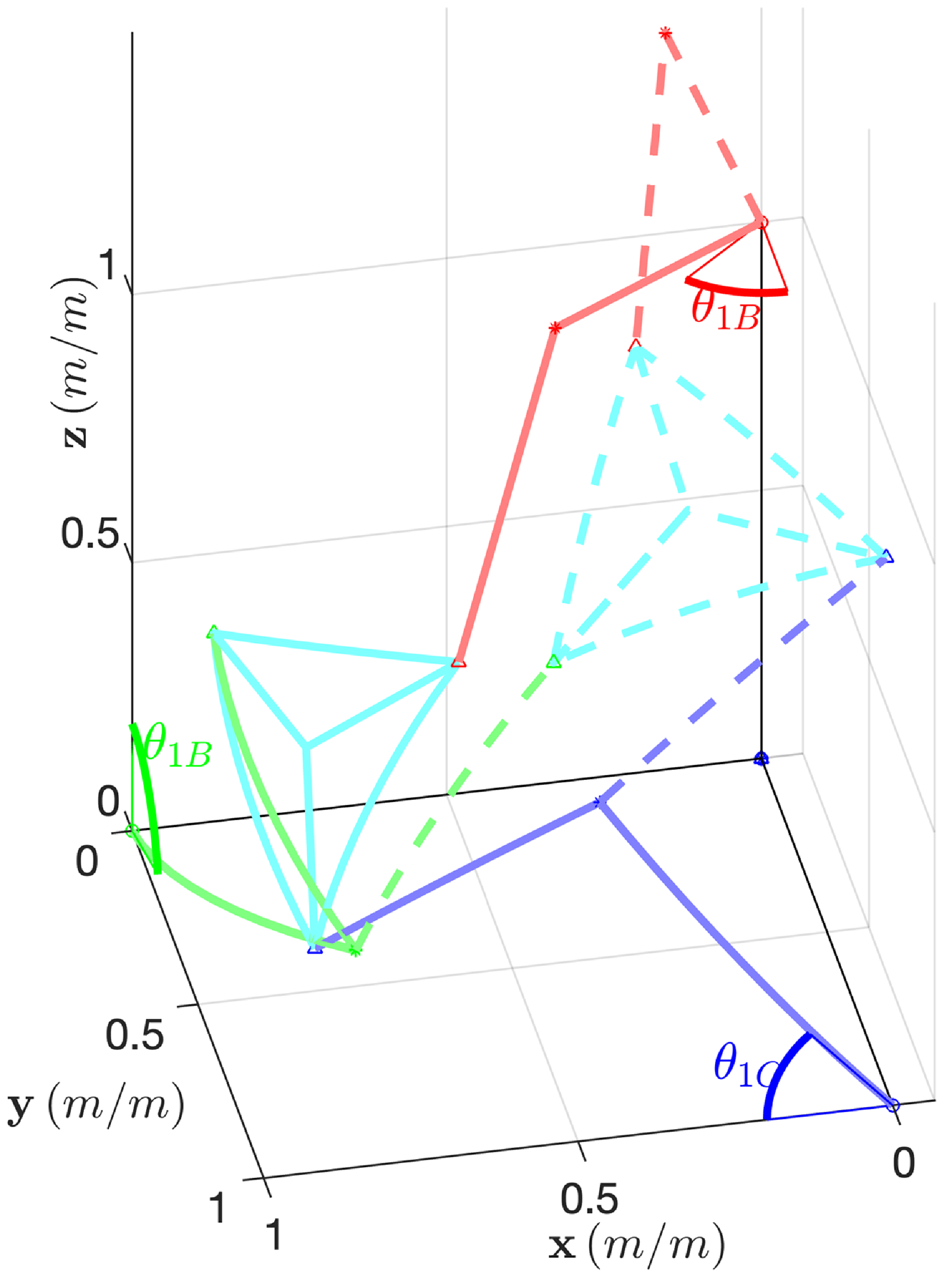
in two sub-dominions, evidencing how the FKM admits more than one solution, that is, working mode, which is a general peculiarity for parallel robots. An example is reported in Figure 16.


An example of intersection between
 $A_1$
and
 $A_2$
in
 $(\theta _{1A}, \theta _{1B}, \theta _{1C}) = (-48,-77,-49) ^{\circ }$
. Therefore, same active angles admit more than one (distinct) working mode:
 $m_1, m_2$
. The resulting configurations are with continuous line for
 $m_1$
and dashed lines for
 $m_2$
. Measures are in
 $(m/m)$
due to scalability described in (M4).

5.3. Observations on dexterity maps enriched with collision
Focusing on Section 4.3, the following observations on
 $W_{reach,c}$
(25), the dexterity maps, in Figures 13 and 23, and the performance indices
 $\delta _{E,min,C_V}$
(26) and
 $\delta _{E,min,\tilde{C}_V}$
(27) in Figure 14, can be made:
-
D4) Due to Assumption (M3), the self-collision phenomenon does not break symmetry;
-
D5)
$\delta _{E,min,\tilde{C}_V}\lt \delta _{E,min,S_J}$
for all working modes with the exception of
$m_{3,7}$
, which is unaffected of any
$\tilde{C}_V$
addition. This is because the working mode’s architecture does not allow any collision of distal links in the operative workspace
$W_{op}$
, as shown in Figure 4g; -
D6) As expected,
$\delta _{E,min,C_V} \leq \delta _{E,min,\tilde{C}_V}$
for all working modes. The equality happens:-
• In parts of
$m_{1,5}$
and
$m_{4,8}$
where the collision phenomenon of the arms and the cylindric volume cannot happen; -
• In
$m_{2,6}$
, in which, as shown in Figure 23, the additional contribution of
$C_V$
with respect to
$\tilde{C}_V$
does not modify the reachable workspace.; -
• In
$m_{3,7}$
for
$|\phi _r| \leq 16 ^{\circ }$
, in which the collision phenomenon between the cylindric volume and the legs happens outside the operative workspace
$W_{op}$
.
-
-
D7) Regarding the overall dexterity in the operative workspace
$W_{op}$
(9), working modes
$m_{2,6}$
, considered the best without collision by Observation (D2), show the worst performance. This is because the working mode’s architecture is particularly sensitive to self-collision between RRR legs, as shown in Figure 4f; -
D8) Considering the previous observations, the best working modes are
$m_{3,7}$
. This is because, as shown in Figure 14,
$m_{3,7}$
are not only symmetrical (D1) (D4) but also record greater distance from singularity regions compared to other modes. In fact, the collision phenomenon only interests the cylindric volume (D5) and for a limited angular range (D6). Consequently, they demonstrate enhanced dexterity and possess the widest reachable workspace.


5.4. Observations on aspects enriched with collision
Focusing on Section 4.4, the following observations on
 $A_i|_{i=(1,\dots, 8),c}$
(28) can be made:
-
E5) Due to Observation (D4), Observation (E1) is still true. In a similar fashion, being the self-collision just an enrichment, the kinematic architecture is not modified and Observation (E3) is still true;
-
E6)
$A_{3,7}$
still intersect both
$A_{1,5}$
and
$A_{4,8}$
in two tangential surface areas, that is, the singularity zones in which one 3-RRR leg is extended; -
E7) Being greatly reduced as a consequence of Observation (D7),
$A_{2,6}$
do not intersect
$A_{1,5}$
nor
$A_{4,8}$
. In fact, the example is reported in Figure 16 is not admissible for the self-collision phenomenon.


5.5. Experimental evaluation of the self-collision mathematical model
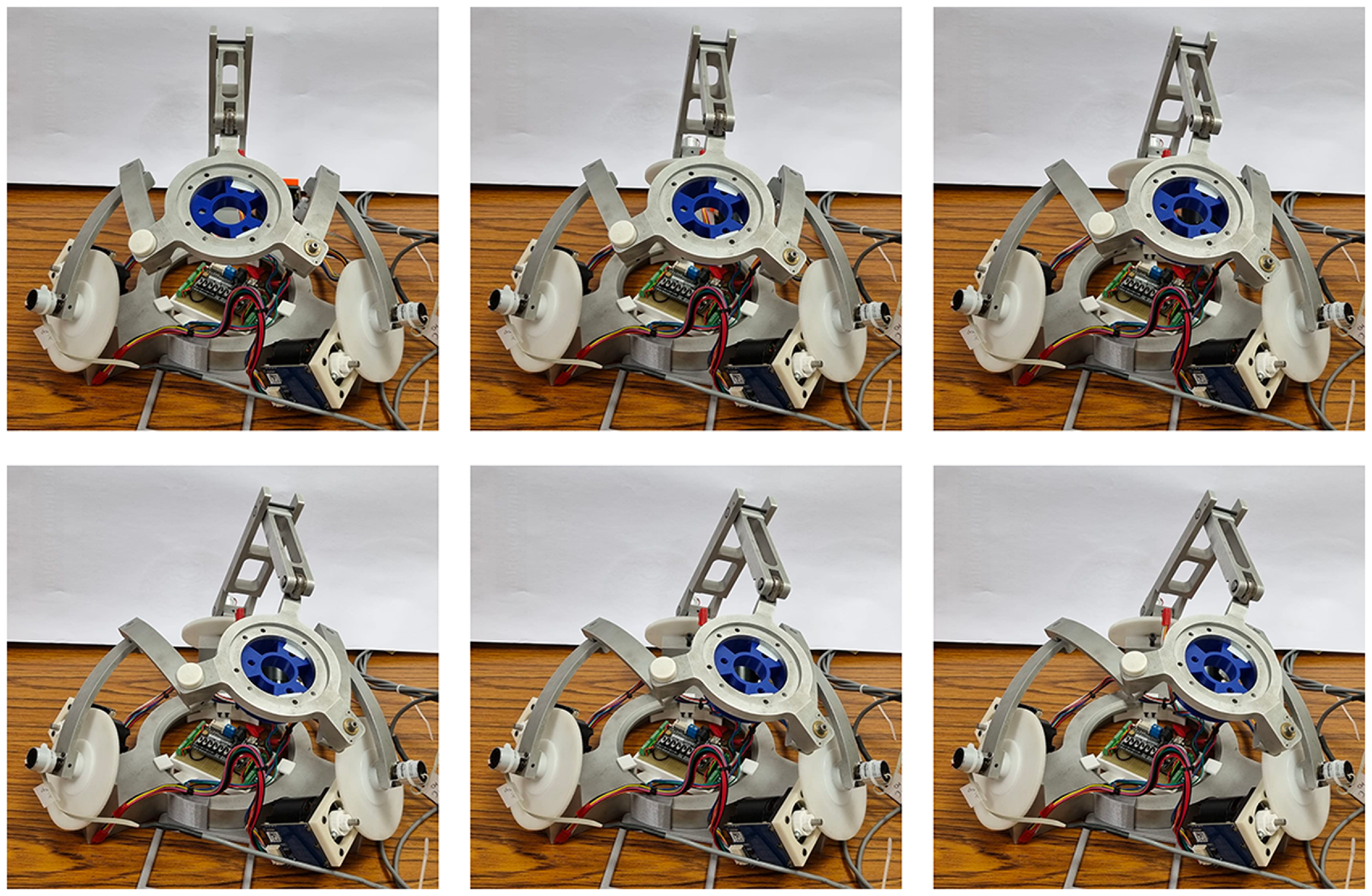
Focusing on the prototype presented in ref. [Reference Saafi, Laribi and Zeghloul20], we have implemented on the architecture the forward kinematic model as in Section 2.5 on the best working mode
 $m_3$
as concluded in Observation (D8). The self-collision mathematical model presented in Section 4 can be efficiently validated by designing a suitable self-colliding trajectory control between the workspace center
 ${\boldsymbol{r}}_{\boldsymbol{wc}}$
(10) and unreachable points
 ${\boldsymbol{P}}_{\boldsymbol{f}}=(\psi _{rf},\theta _{rf},\phi _{rf}) \in C_V$
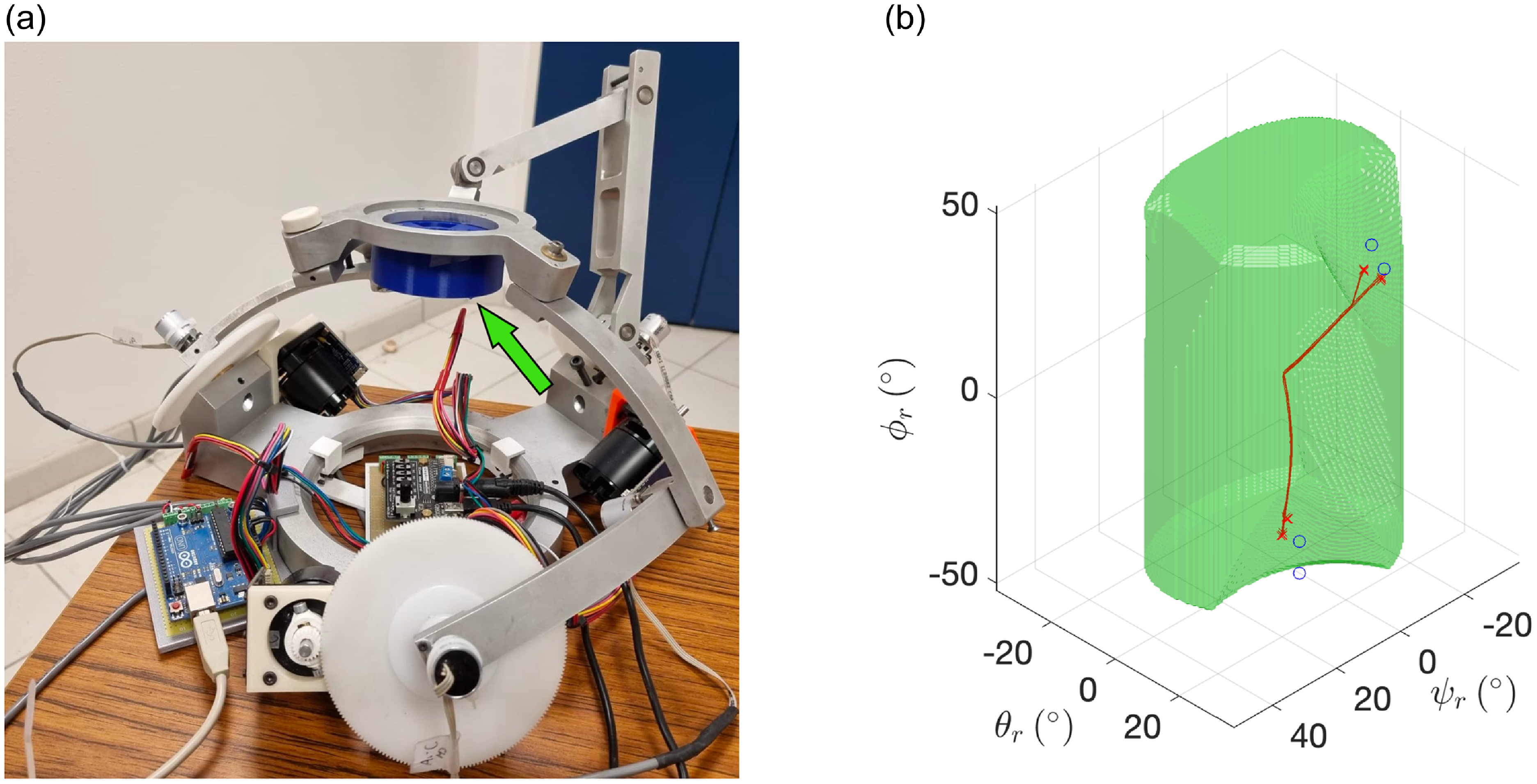
(23). Therefore, the prototype is made to collide with a proper 3D-printed cylindric volume mounted on the platform, as in Figure 17a.
Registering the absorbed current on the actuated motors (Simplex Motion, SC040B), as defined in Section 2.1, the collision is checked by monitoring the feedback torques and is demonstrated to happen on the threshold surface of
 $W_{reach,c}$
, as shown in Figure 17b. Four tested self-colliding trajectories, each one tested five times, are presented in Table I with their averaged collision points
 $\bar{\boldsymbol{P}}_{\boldsymbol{C}}=(\bar{\psi }_{rC},\bar{\theta }_{rC},\bar{\phi }_{rC})$
and their respective euclidean distance from
 $W_{reach,c}$
threshold surface
 $d_{wrs}$
.
Cylindric object (in blue, highlighted with an arrow) mounted on the platform of the prototype [Reference Saafi, Laribi and Zeghloul20] (a); reachable workspace within the Euler dominion
 $W_{reach,c}$
for
 $m_3$
(in green) with four self-colliding trajectories (in red, with blue
 $O$
marker pointing the referenced trajectory final points inside
 $C_V$
, and red
 $\times$
markers pointing the collision) (b).

A discrete frame-by-frame photographic representation of the first trajectory is exemplified in Figure 24 in Appendix.
5.6. Self-collision avoidance algorithm
In order to implement a self-collision avoidance algorithm, we must act on
 $\boldsymbol{\tau}_{\boldsymbol{ctrl}}$
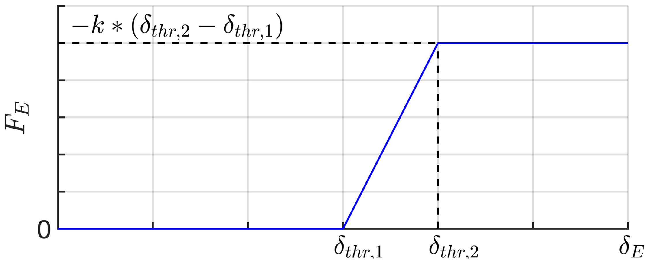
defined in (8), that is, the torque on the active angles regulating control actions which involve only the master device. This article proposes a segmented spring-like avoidance algorithm, acting on
 $W_{reach,c}$
, as in (29), (30), (31), and Figure 18.
 \begin{equation} {\boldsymbol{F}}_{\boldsymbol{E}} = \begin{cases} \begin{aligned} \underline{\textbf{0}} & \quad &\delta _E \leq \delta _{thr,1}\\[5pt] -k_\delta \cdot (\delta _E-\delta _{thr,1}) \cdot {\boldsymbol{t}}_{\boldsymbol{E}} & \quad & \delta _{thr,1} \lt \delta _E \leq \delta _{thr,2}\\[5pt] -k_\delta \cdot (\delta _{thr,2}-\delta _{thr,1}) \cdot {\boldsymbol{t}}_{\boldsymbol{E}} & \quad & \delta _E \geq \delta _{thr,2}\\[5pt] \end{aligned} \end{cases} \end{equation}
 \begin{equation} {\boldsymbol{M}}_{\boldsymbol{E}} = \begin{cases} \begin{aligned} \underline{\textbf{0}} & \quad &|\phi _r| \leq \phi _{thr,1}\\[5pt] -k_\phi \cdot (\phi _r-\phi _{thr,1}) \cdot {\boldsymbol{r}}_{\boldsymbol{E}} & \quad & \phi _{thr,1} \lt |\phi _r| \leq \phi _{thr,2}\\[5pt] -k_\phi \cdot (\phi _{thr,2}-\phi _{thr,1}) \cdot {\boldsymbol{r}}_{\boldsymbol{E}} & \quad & |\phi _r| \geq \phi _{thr,2}\\[5pt] \end{aligned} \end{cases} \end{equation}
 \begin{equation} \boldsymbol{\tau}_{\boldsymbol{ctrl}} = J^t \cdot {\boldsymbol{T}}_{\boldsymbol{ctrl}} = J^t \cdot ( r_p{\boldsymbol{r}}_{\boldsymbol{E}} \boldsymbol\times {\boldsymbol{F}}_{\boldsymbol{E}} + {\boldsymbol{M}}_{\boldsymbol{E}}) \end{equation}
Four tested self-colliding trajectories specifications (all values in
 $[^{\circ }]$
).


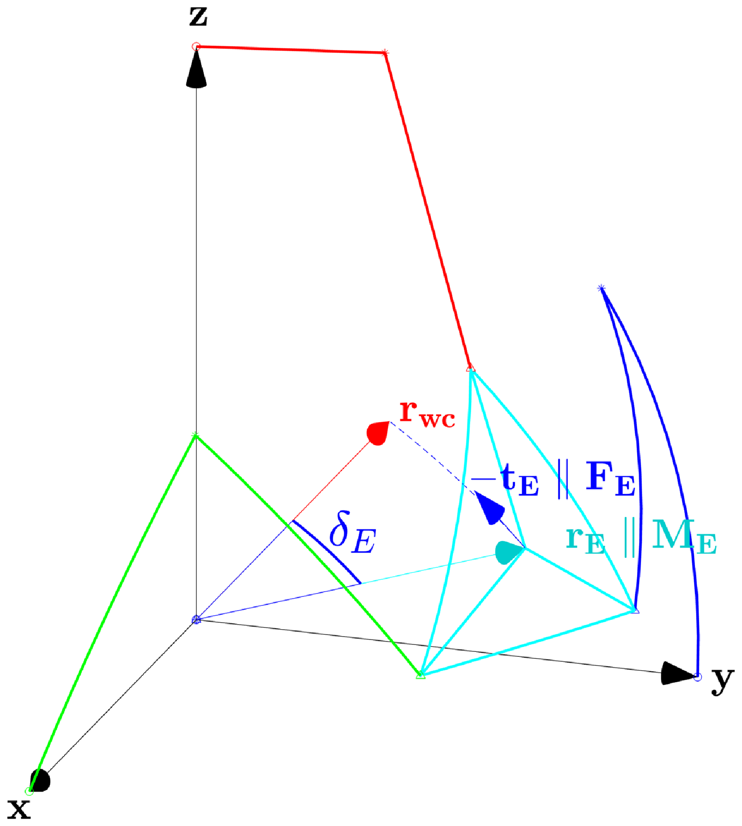
In which, as in Figure 19:
 ${{\boldsymbol{T}}_{\boldsymbol{E}}}$
and
 ${\boldsymbol{M}}_{\boldsymbol{E}}$
are the requested force and torque acting on the device in order to control, respectively, its angular distance
 $\delta _E$
from the workspace center
 ${\boldsymbol{r}}_{\boldsymbol{wc}}$
(10) (12) and its self-rotation angle
 $\phi$
;
 $k_\delta$
and
 $k_\phi$
are suitable spring constants;
 $\delta _{thr,1,2}$
and
 $\phi _{thr,1,2}$
are suitable threshold values;
 ${\boldsymbol{t}}_{\boldsymbol{E}}$
is the unitary vector perpendicular to
 ${\boldsymbol{r}}_{\boldsymbol{E}}$
lying on the plane
 $({\boldsymbol{r}}_{\boldsymbol{wc}}, {\boldsymbol{r}}_{\boldsymbol{E}})$
to maximize
 ${\boldsymbol{F}}_{\boldsymbol{E}}$
work (32);
 $r_p \, (m)$
is the actual distance between the EE center of mass and the RF origin, reported in Table II.
 \begin{equation} {{\boldsymbol{t}}_{\boldsymbol{E}} = {\boldsymbol{r}}_{\boldsymbol{E}} \boldsymbol\times ({\boldsymbol{r}}_{\boldsymbol{E}} \boldsymbol\times {\boldsymbol{r}}_{\boldsymbol{wc}})} \end{equation}
While
 $\phi _{thr,1,2}$
can be directly imposed considering
 $W_{op}$
(9),
 $\delta _{thr,1,2}$
cannot be set a-priori, since they are directly influenced by
 $W_{reach,c}$
(25). The proposed solution relies on the a-priori computation of a normalized force map in every point of
 $W_{reach,c}$
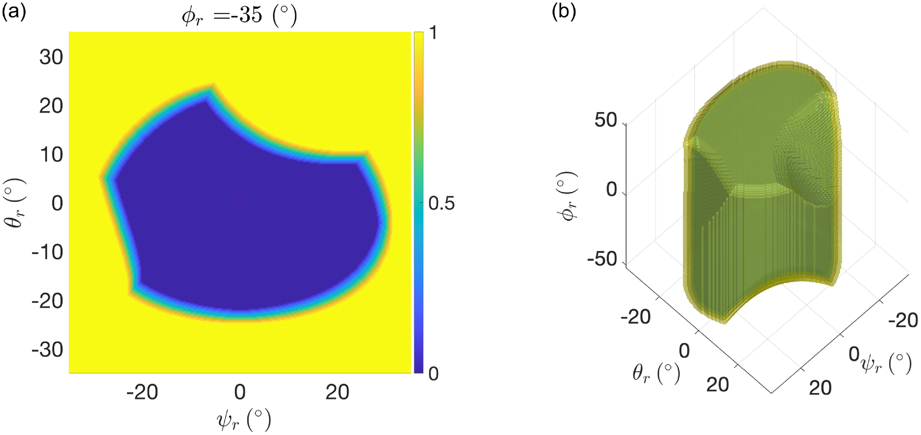
in the Euler space, as in (33) and Figure 20.
 \begin{equation} {\boldsymbol{F}}_{\boldsymbol{E}} = |F_{E,max}| f_{E,map}(\psi _r,\theta _r,\phi _r) \cdot {\boldsymbol{t}}_{\boldsymbol{E}} \end{equation}
In which:
 $|F_{E,max}|$
is the imposed maximum spring-like force;
 $0 \leq f_{E,map}(\psi _r,\theta _r,\phi _r) \leq 1$
is the normalized force map, unitary outside of
 $W_{reach,c}$
(25), and null inside a proper subset of it, as to implement
 $\delta _{thr,1,2}$
in (29).
Parameter values used for the IKM, FKM, and the self-collision phenomenon.

Normalized force map
 $f_{E,map}(\psi _r,\theta _r,\phi _r)$
in the plane
 $\psi _r\theta _r$
for
 $m_{3,7}$
and
 $\phi _r = -35 ^{\circ }$
(a) and in the overall Euler space (b). Offset
 $\delta _{thr,2}-\delta _{thr,1} = 3 ^{\circ }$
.

Once
 $f_{E,map}(\psi _r,\theta _r,\phi _r)$
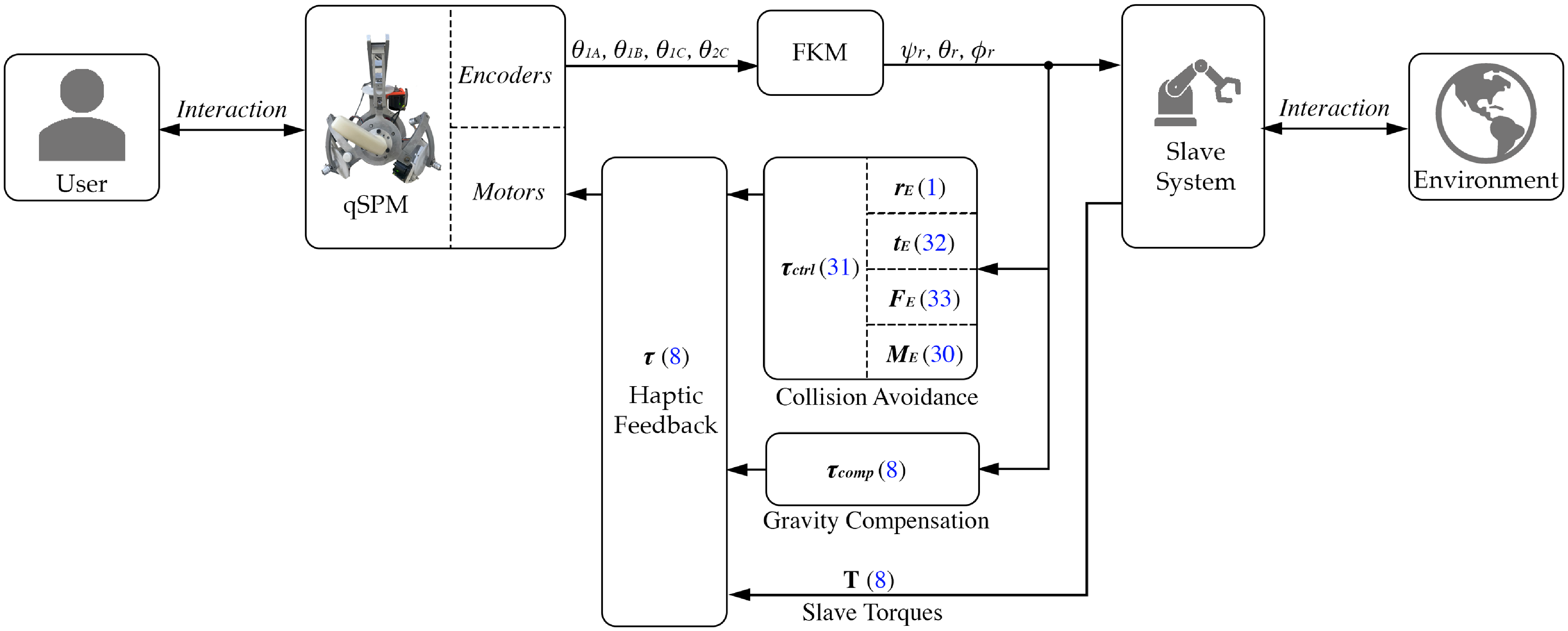
is computed offline, it can directly implement a collision avoidance control action through the use of the FKM, as in Section 2.5, and the computation of (8), (30), (31), (32), and (33), as schematized in Figure 21. Having an offline force map means that singularity areas
 $S_J$
(14) and self-collision points
 $C_V$
(23) are detected a priori, generating a suitable control action for the motors to keep the EE inside the reachable workspace (25).
Overall control scheme of the qSPM, including the collision avoidance action. All numbered labels refer to the respective equations presented in the article.

6. Conclusions
This article was devoted to a comprehensive analysis of the qSPM, a three-legged parallel robot with two spherical RRR legs and one nonspherical URU leg.
After presenting the mathematical definition of the prototype, laying out insights on inverse and forward kinematics, the Jacobian matrix, and the haptic feedback, the research has focused on the dominion analysis of the operative and reachable workspaces due to singularity areas, and introducing the concept of aspects within its joint space. All presented dominions were enriched by considering the phenomenon of self-collision, which was analytically presented, delineating a restricted reachable workspace by identifying self-collision critical points. The article has then discussed the differences among the dominions. In fact, working modes
 $m_{2,6}$
, appearing as the most suitable ones without the self-collision phenomenon description, were discarded in favor of
 $m_{3,7}$
, left unbiased by the phenomenon due to their peculiar architecture.
The self-collision phenomenon was experimentally evaluated on working mode
 $m_3$
, proposing a segmented spring-like avoidance algorithm in order to always remain inside the reachable workspace.
Future developments will revolve around haptic feedback control validation and the self-collision avoidance algorithm optimization, partaken on a prototype within a test-bench framework and a simulation environment implementing digital twins of both the master and slave robots.
Author contributions
LMA and PQD conceived and designed the study. PQD wrote the article. LMA and MD contributed to the revision process.
Financial support
This research received no specific grant from any funding agency, commercial or not-for-profit sectors.
Competing interests
The authors declare no conflicts of interest exist.
Ethical approval
None.
A. Appendix
For sake of clarity, notation
 $(cos(x)= c_x \,,\,sin(x)=s_x)$
has been adopted.
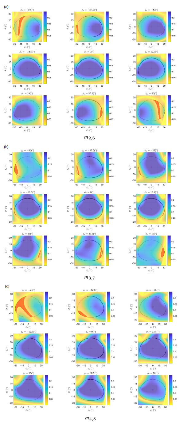
Dexterity map in the Euler angles space for
 $m_{2,6}, \, m_{3,7}, \, m_{4,8}$
. Planes
 $\psi _{r}\theta _{r}$
range with a discrete-step of
 $\phi _{r,step} =12.5^{\circ }$
. Relative angles defined in (11). Red areas correspond to singularity areas
 $S_J$
(14) inside the operative workspace
 $W_{op}$
(9).

 \begin{equation} \begin{cases} \begin{alignedat}{2} A_1&= c_{\gamma } s_{\psi } s_{\theta } - s_{\gamma } (c_{\psi } s_{\phi } + s_{\psi } c_{\theta } c_{\phi }) \\[5pt] A_2&= - c_{\gamma } c_{\psi } s_{\theta } - s_{\gamma } (s_{\psi } s_{\phi } - c_{\psi } c_{\theta } c_{\phi } ) \\[5pt] A_3&= 0 \end{alignedat} \end{cases} \end{equation}
 \begin{equation} \begin{cases} \begin{alignedat}{2} B_1&= s_{\alpha } [c_{\gamma } c_{\theta } - \tfrac{1}{2} s_{\gamma } s_{\theta } (c_{\phi } + \sqrt{3} s_{\phi })] \\[5pt] B_2&= s_{\alpha } \{ c_{\gamma } c_{\psi } s_{\theta } + \tfrac{1}{2} s_{\gamma } [c_{\phi } (c_{\psi } c_{\theta } + \sqrt{3} s_{\psi }) + s_{\phi } (- s_{\psi } + \sqrt{3} c_{\psi } c_{\theta })] \} \\[5pt] B_3 &= c_{\alpha } \{ c_{\gamma } s_{\psi } s_{\theta } + \tfrac{1}{2} s_{\gamma } [c_{\phi } (s_{\psi } c_{\theta } - \sqrt{3} c_{\psi }) + s_{\phi } (c_{\psi } + \sqrt{3} s_{\psi } c_{\theta })] \} - c_{\beta } \end{alignedat} \end{cases} \end{equation}
 \begin{equation} \begin{cases} \begin{alignedat}{2} C_1&= s_{\alpha } \{c_{\gamma } s_{\psi } s_{\theta } + \tfrac{1}{2} s_{\gamma } [c_{\phi } (s_{\psi } c_{\theta } +\sqrt{3} c_{\psi }) + s_{\phi } (c_{\psi } -\sqrt{3} s_{\psi } c_{\theta })] \} \\[5pt] C_2&= s_{\alpha } [ - c_{\gamma } c_{\theta } + \tfrac{1}{2} s_{\gamma } s_{\theta } (c_{\phi } - \sqrt{3} s_{\phi }) ] \\[5pt] C_3&= c_{\alpha } \{ - c_{\gamma } c_{\psi } s_{\theta } + \tfrac{1}{2} s_{\gamma }[c_{\phi } (- c_{\psi } c_{\theta } + \sqrt{3} s_{\psi }) + s_{\phi } (s_{\psi } + \sqrt{3} c_{\psi } c_{\theta })] - c_{\beta } \end{alignedat} \end{cases} \end{equation}
 \begin{equation} \begin{cases} \begin{alignedat}{2} x_{Ki} |_{K =(B,C), i = (1,2)} &= -\frac{1}{K_1} \cdot (K_3 \mp (K_2 \cdot \frac{K_1 \cdot \sqrt{K_1^2+K_2^2-K_3^2} \pm K_2 \cdot K_3}{K_1^2+K_2^2})) \\[5pt] y_{Ki} |_{K =(B,C), i = (1,2)} &= \mp \frac{K_1 \cdot \sqrt{K_1^2+K_2^2-K_3^2} \pm K_2 \cdot K_3}{K_1^2+K_2^2} \end{alignedat} \end{cases} \end{equation}
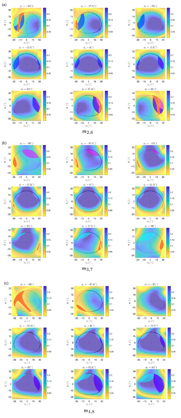
Dexterity map in the Euler angles space for
 $m_{2,6}, \, m_{3,7}, \, m_{4,8}$
. Planes
 $\psi _{r}\theta _{r}$
range with a discrete-step of
 $\phi _{r,step} =12.5^{\circ }$
. Relative angles defined in (11). Colored areas correspond, respectively, to singularity areas
 $S_J$
(red) (14) and collision areas
 $C_V$
(blue:
 $C1$
, cyan:
 $C2$
, magenta:
 $C3$
as in Section 4.2) (23) inside the operative workspace
 $W_{op}$
(9).

Discrete frame-by-frame photographic representation of the first collision trajectory adopted in Section 5.5.