1. Introduction
The role of financial regulation in maintaining financial stability during the green transition is gaining increasing attention, as it shapes the resilience of the financial system during structural economic changes. While fiscal policy leads climate initiatives, growing interest focuses on how financial regulation through collateral frameworks, and similar tools can complement these efforts. Although these policy measures are designed with long-term objectives in mind, they also have significant short-run implications for the business cycle, which are the main focus of this paper. We propose a nonlinear macro-finance model to analyze the interaction between fiscal policy and financial regulation to identify stability-preserving policy mixes.
Existing literature often offers a limited view by focusing on single regulations, abstracting from nonlinear interactions between policies, neglecting short-run implications and, in particular, the crucial role of credit markets and their inherent instability. We address these gaps by using a nonlinear overlapping generations (OLG) model, building on Matsuyama (Reference Matsuyama2013) and Matsuyama et al. (Reference Matsuyama, Sushko and Gardini2016), in which credit cycles emerge endogenously without exogenous shocks. We extend this framework by incorporating an environmental dimension, following Caravaggio and Sodini (Reference Caravaggio and Sodini2018), and introducing two regulatory authorities. At the core of this modeling framework are intergenerational externalities of production and sectoral asymmetries. In each period, young agents supply labor and earn wage income, which they save entirely.
When turning old, agents allocate their accumulated net worth among green projects, brown projects, and lending in the credit market. At the end of their life, they consume the returns from these investments. Green projects employ capital from the older generation and labor from the young, thereby generating intergenerational spillovers, and additionally use environmental resources as inputs. These projects face no binding financial constraints. In contrast, brown projects lack such positive spillovers, relying solely on capital from the older generation. Agents initiating the latter must obtain financing in a competitive capital market, pledging expected returns as collateral – a process shaped by the financial regulator. The higher their net worth, the less external finance they require. Moreover, brown projects emit pollution, imposing a negative externality on subsequent green production, and are subject to taxation set by the government. Note that the specific sectoral asymmetries generate endogenous cycles. Investment in the green sector raises net worth, thereby facilitating the financing of brown projects. However, investment in brown projects diverts credit away from the green sector, causing the next generation’s net worth to decline again. This design allows us to study how fiscal and financial regulation influence the joint dynamics of capital, credit, and the environment in a business cycle setting.
Our model features two types of environmental regulation. Financial regulation tightens financing conditions for brown projects by applying an environmental haircut to collaterals, thereby reducing the feasibility of new brown investments, lowering emissions, and improving environmental quality. While such measures are often associated with monetary policy authorities, our framework remains general and is not tied to a specific institution, provided that the entity can adjust the collateral framework governing credit access. In contrast, fiscal environmental regulation imposes a tax on brown projects, diminishing their profitability, curbing their numbers and thus emissions. The revenues generated from this tax can be directed toward abatement technologies or direct environmental investments, with positive effects on the environment. In combination, these regulatory tools constrain the expansion of the brown sector and redirect credit flows toward green investments.
While the model remains sufficiently simple for analytical treatment, it includes all necessary components to address the following research questions: How do fiscal and financial policies affect the income and environmental quality of the economy? Are there trade-offs or interaction effects between the two types of regulation on system stability? Finally, how does environmental regulation affect the distribution of income across generations, especially between younger and older agents?
Our model allows for a partial analytical assessment of fixed-point stability, which is complemented by numerical simulations to capture the effects of policy interactions. We show that financial regulation, via environmental haircuts, reduces financing for brown projects and redirects investment toward green alternatives. Yet, environmental outcomes remain ambiguous: fewer brown projects lower emissions but also cut tax revenues, limiting funds for abatement and environmental improvement. Green fiscal policy, through environmental taxes, discourages brown projects while generating revenue for improvements, though its effectiveness depends on revenue allocation, producing non-monotonic effects on both the environment and income distribution. Individually, both policies risk destabilizing dynamics, but in combination they can reduce fluctuations, yielding comparable average levels of environmental quality and income. From a distributional perspective, we identify generational conflicts: tighter environmental regulation often raises environmental quality and income of the young generation, but it reduces and destabilizes the incomes of the old, highlighting a trade-off between environmental quality and intergenerational equity.
The remainder of the paper is structured as follows. Sections 2 and 3 offer an overview of relevant literature and stylized facts that motivate our core assumptions. Section 4 introduces the model framework, discusses its global dynamics, and provides numerical simulations. Section 5 discusses the macroeconomic implications of the two regulatory approaches, while Section 6 examines their effects on income distribution. Section 7 concludes.
2. Related literature and modeling aspects
There exists a strand of literature that integrates environmental aspects into macroeconomic models, typically with a long-run perspective that abstracts from shorter-term business cycle dynamics. A foundational contribution stems from Nordhaus’s integrated assessment models (IAMs; see most recently, Barrage and Nordhaus, Reference Barrage and Nordhaus2024), which have been widely employed in policy evaluations (e.g., Golosov et al., Reference Golosov, Hassler, Krusell and Tsyvinski2014; Hassler et al., Reference Hassler, Krusell, Olovsson and Reiter2020). IAMs generally capture environmental degradation through a damage function that explicitly links aggregate productivity to an environmental indicator, such as global temperature (see, e.g., Bastien-Olvera and Moore, Reference Bastien-Olvera and Moore2021), with recent work providing microfoundations and estimation (Caggese et al., Reference Caggese, Chiavari, Goraya and Villegas-Sanchez2024).Footnote 1
Closer to our modeling approach are OLG models, that feature two principal approaches to capture how environmental quality affects production. The first approach employs a damage function that reduces aggregate productivity (e.g., Dao et al., Reference Dao, Burghauser and Edenhofer2017), whereas the second, which we adopt, treats environmental resources directly as production inputs (Smulders and Gradus, Reference Smulders and Gradus1996; Caravaggio and Sodini, Reference Caravaggio and Sodini2018). Most of these models focus on long-run growth and omit financial sectors as endogenous sources of cyclical fluctuations. By contrast, our framework centers on short-run business-cycle dynamics driven by financial markets and regulatory interventions.
Environmental policy also interacts with the financial sector, especially during the green transition. Recent literature explores how monetary policy and financial regulations can support these transitions, mainly within dynamic stochastic general equilibrium (DSGE) frameworks (see, e.g., Holtemöller and Sardone, Reference Holtemöller and Sardone2024; Chan et al., Reference Chan, Ji and Zhang2024; Dietrich et al., Reference Dietrich, Müller and Schoenle2022). Predominantly, tools such as green quantitative easing (QE) are investigated (Abiry et al., Reference Abiry, Ferdinandusse, Ludwig and Nerlich2022; Ferrari and Nispi Landi, Reference Ferrari and Nispi Landi2024).Footnote 2 In such models, business-cycle dynamics are typically driven by exogenous shocks. Recognizing the intrinsic instability of financial markets, we depart from these approaches by employing a framework explicitly featuring endogenous credit dynamics.
Our modeling strategy builds upon the finding that the financial sector is inherently unstable and subject to endogenous fluctuations (see, e.g., Minsky, Reference Minsky1986; Chiappori and Guesnerie, Reference Chiappori and Guesnerie1988; Boldrin and Woodford, Reference Boldrin and Woodford1990; Azariadis and Smith, Reference Azariadis and Smith1998; Aghion et al., Reference Aghion, Banerjee and Piketty1999), specifically extending the endogenous credit-cycle models introduced by Matsuyama (Reference Matsuyama2013), Matsuyama et al. (Reference Matsuyama, Sushko and Gardini2016). These models show how financial frictions can generate endogenous cycles in financial markets, building on earlier work that established such frictions as fundamental drivers of business cycle fluctuations (e.g., Bernanke and Gertler, Reference Bernanke and Gertler1989; Kiyotaki and Moore, Reference Kiyotaki and Moore1997; Gilchrist and Zakrajšek, Reference Gilchrist and Zakrajšek2012). The financial friction in our base model, following Matsuyama et al. (Reference Matsuyama, Sushko and Gardini2016), arises because only a fraction of an investment’s expected return can be pledged as collateral (i.e., it is subject to a haircut) thereby limiting access to credit financing.
Finally, our model captures both inter- and intra-generational inequality by distinguishing between capitalists and workers, as well as between young and old agents. This structure follows the tradition of OLG and credit-cycle models that explore income distribution dynamics (Kubin and Zörner, Reference Kubin and Zörner2021; Bougheas et al., Reference Bougheas, Commendatore, Gardini, Kubin and Zörner2025). By incorporating these features, we also contribute to the growing literature examining how environmental and energy policies influence economic inequality (Känzig, Reference Känzig2023; Pieroni, Reference Pieroni2023; Chan et al., Reference Chan, Ji and Zhang2024).
3. Environmental policy and sectoral asymmetries
This section discusses some observations motivating our model’s assumptions. We first document the increasing integration of environmental objectives into fiscal and monetary policy, emphasizing the growing role of both climate-related fiscal policies and green financial regulation. We then present stylized facts supporting our green–brown project distinction, a central feature of the framework that generates asymmetric regulatory impacts on sectoral dynamics.
3.1 Relevance of Climate-related Policies
Empirical evidence highlights the increasing relevance of climate-related policies among both fiscal and monetary authorities. Governments have progressively integrated climate change mitigation into their agendas, employing a range of instruments such as Pigouvian taxes (Baiardi and Menegatti, Reference Baiardi and Menegatti2011) and public investments in abatement technologies (Porter and van der Linde, Reference Porter and van der Linde1995; Brock and Taylor, Reference Brock and Taylor2010). As shown in Figure 1a, the number of environmental policies implemented across OECD countries from 1990 to 2022 exhibits a clear upward trend. Existing literature emphasizes that these instruments typically take the form of direct regulation (e.g., setting minimum standards or prohibiting inputs) and the taxation of polluters. In parallel, financial markets and monetary authorities have increasingly acknowledged climate-related risks. Survey evidence shows that while regulatory risk is perceived as the dominant concern in the near term, physical climate risks are expected to become more important in the long run, with asset prices widely believed to underestimate these risks (Stroebel and Wurgler, Reference Stroebel and Wurgler2021). Central banks, in particular, are devoting greater attention to the potential threats climate change poses to financial stability. This growing emphasis is also reflected in their public communication, as shown by Campiglio et al. (Reference Campiglio, Deyris, Romelli and Scalisi2025), who document a significant rise in climate-related discourse across central banks over recent decades. Figure 1b illustrates this shift: while Federal Reserve officials have integrated climate-related topics only moderately, nearly all recent ECB speeches include explicit references to climate change, indicating a stronger commitment to embedding environmental considerations into European monetary discourse.
Fiscal and monetary policy makers and climate change.
Notes: Panel (a) displays the annual aggregate number of climate mitigation policies adopted across various sectors or policy areas within OECD countries from 1990 to 2022. The policies are categorized into market- and non-market-based instruments, covering the electricity, building, transport, and industry sectors, as well as cross-sectoral and international policies (Source: OECD Climate Action Dashboard). Panel (b) illustrates the proportion of speeches by officials from the Federal Reserve (light gray) and ECB (dark gray) that addressed green topics, spanning from 1999 to May 2023 (Source: Speech database of Fed and ECB).

3.2 Sectoral Heterogeneity and the Polluting Brown Sector
Our model structure embeds the environmental externality into an OLG framework with endogenous credit cycles, in which sectoral heterogeneity is a core element. In our framework, the labor-intensive sector is non-polluting, whereas only the capital-intensive sector generates emissions. This distinction between a green and a brown sector is motivated by three considerations: capital intensity, financing frictions, and the environmental footprint of final consumption.
First, empirical evidence suggests a positive association between capital intensity and environmental pollution. Studies such as Antweiler et al. (Reference Antweiler, Copeland and Taylor2001), Cole and Elliott (Reference Cole and Elliott2003), Cole et al. (Reference Cole, Elliott and Shimamoto2005), Dietzenbacher and Yan (Reference Dietzenbacher and Yan2024) find that sectors with higher physical capital requirements, such as heavy industry and fossil fuel extraction, tend to generate disproportionately high emissions. In line with this evidence, we model the brown sector as highly capital-intensive, relying exclusively on capital in its production technology, while the green sector combines capital and labor. Cole and Elliott (Reference Cole and Elliott2005) also highlight the importance of high capital expenditures in relation to pollution. In a broader study that includes additional explanatory variables, Agnolucci and Arvanitopoulos (Reference Agnolucci and Arvanitopoulos2019) confirm the role of high capital expenditures among other contributing factors, although they cannot corroborate the role of physical capital input.
Second, in our model one sector requires external finance through collateralized credit. Above, we argued that monetary authorities and financial markets increasingly account for climate-related risks and polluting (brown) sectors typically face greater difficulties in accessing finance. Consistent with this stylized fact, we assume that projects relying on collateral-backed credit are those in the brown, polluting sector, whereas green projects are not subject to such financing frictions. Recent empirical evidence supports this assumption, showing an increasing divergence in financing conditions: sustainable investing has significantly lowered the cost of capital for green projects while raising relative financing costs for brown firms (Gormsen et al., Reference Gormsen, Huber and Oh2024; Chen and Takahashi, Reference Chen and Takahashi2024).
In our model we interpret these financing frictions as potential instruments for green financial regulation. One prominent example is the adjustment of collateral frameworks by central banks, such as the ECB’s planned 2024 reform that explicitly restricts collateral eligibility for assets issued by firms with high carbon footprints (Beckmann et al., Reference Beckmann, Gern, Jannsen and Sonnenberg2023).Footnote 3 Another example is Giovanardi et al. (Reference Giovanardi, Kaldorf, Radke and Wicknig2023), who analyze the use of “green haircuts” as financial policy tools (and find them beneficial, albeit potentially less effective than direct carbon taxation). Unlike their setup, which treats pollution at an aggregate level, our model explicitly differentiates between sectors. For financing projects in the brown sector, investors must pledge their expected returns as collateral, with financial constraints applying specifically to this sector. This is similar to Raberto et al. (Reference Raberto, Ozel, Ponta, Teglio and Cincotti2019), who examine how differentiated capital requirements can redirect investments toward greener sectors, aligning closely with our focus on sector-specific financial regulation.
Third and finally, the two sectors differ fundamentally in how their outputs are used. Output from the green sector serves as an investment good, funding both green and brown projects, as well as a consumption good for older agents who previously invested in green projects. In contrast, output from the brown sector is exclusively used for final consumption by older agents who have either invested directly in brown projects or provided credit to them. This asymmetry is particularly relevant from an environmental standpoint, as empirical studies consistently demonstrate that final consumption activities generate a significantly larger ecological footprint than investment activities, especially when consumption involves energy-intensive goods and services (e.g., Wiedmann et al., Reference Wiedmann, Minx, Barrett and Wackernagel2006; Ivanova et al., Reference Ivanova, Stadler, Steen-Olsen, Wood, Vita, Tukker and Hertwich2016). Thus, our model structure reflects the stylized fact that the brown sector produces exclusively for consumption and thus contributes disproportionately to environmental degradation.
Taken together, these arguments justify modeling the capital-intensive and consumption-oriented sector that is subject to financial frictions as the polluting sector. We acknowledge that alternative approaches exist for modeling sectoral heterogeneity and pollution profiles, but our framework deliberately focuses on the interaction of financial market frictions with fiscal and financial regulation. This focus allows us to analyze how credit dynamics and regulatory instruments jointly shape both macroeconomic stability and environmental outcomes.
4. A credit cycle model with an environment
In this section, we present our model framework, based on Matsuyama et al. (Reference Matsuyama, Sushko and Gardini2016), and outline our approach to modeling the environment within this framework. We then introduce the two regulatory authorities – one fiscal and one financial – and describe the mechanisms. Following this, we provide the dynamic map of the piecewise-smooth system and proceed with an analytical and numerical treatment to explore the global dynamics.
4.1 Production and investment choices
The model adopts an overlapping generations framework (Diamond, Reference Diamond1965) with two period lives where a unit measure of agents arrives at each point of time
 $t=0,1,2,\ldots$
.Footnote
4
The model features two sectors, a green and a brown sector, and an environment that is subject to pollution. In each period a final good, the numeraire, is produced in the green sector which can be used for investments or for consumption. The green goods sector uses the following Cobb-Douglas technology
 \begin{equation*} Y_{t}=Z E_{t}^{\gamma }K_{t}^{\alpha }L_{t}^{1-\alpha }, \end{equation*}
where
 $Y_{t}$
represents the final good produced at time
 $t$
,
 $Z$
denotes total factor productivity,
 $E_{t}$
is the environmental resource, and
 $K_{t}$
and
 $L_{t}$
represent physical capital and labor, respectively. Here,
 $\gamma \lt 1$
is the elasticity of output with respect to the environmental resource, while
 $\alpha \lt 1$
represents share of capital in production (i.e., the elasticity of output with respect to production). The environment is a freely usable aggregate resource that positively influences the productivity of the other input factors. It is not privately owned, and agents do not anticipate its aggregate development in their decision-making, nor do they consider the impact of their actions on this resource. Implementing the normalization
 $Z(1-\alpha )=1$
, competitive factor markets yield the following factor remunerations for capital and labor, respectively, depending on
 $k_t=\frac {K_{t}}{L_{t}}$
,
 \begin{equation} \rho _{t} = f^{\prime }(k_{t}) = \frac {\alpha }{1-\alpha }E_{t}^{\gamma } K_{t}^{\alpha -1} L_{t}^{1-\alpha } = \frac {\alpha }{1-\alpha } E_{t}^{\gamma } k_{t}^{\alpha -1} \end{equation}
and
 \begin{equation} w_{t} = f(k_{t})-k_{t}f^{\prime }(k_{t})= E_{t}^{\gamma } K_{t}^{\alpha } L_{t}^{1-\alpha } = E_{t}^{\gamma } k_{t}^{\alpha }. \end{equation}
Note that
 $\rho _{t}$
is decreasing and
 $w_{t}$
is increasing in
 $k_{t}$
, and the environmental resource
 $E_{t}$
is not measured in units of labor. The environmental resource enhances the returns to the other two inputs.
Each period, a new measure of agents arrives (is born) and stays active for two periods. In the first period, young agents provide one unit of labor and earn the net worth
 $w_{t}$
. They save everything and face an investment decision at the end of period one to maximize their consumption at the end of the second period (when they are old). To allocate their net worth, they can choose from three options: investing in one of two projects (green or brown) or supplying credit through competitive, albeit imperfect, capital markets.
Investing in the green sector that uses the final good as capital input for the next period as
 $k_{t+1}$
, is expected to yield a return equal to the marginal product of capital,
 $\rho _{t+1},$
under the assumption of perfect foresight. Green projects fuel production processes and have a positive intergenerational spillover: They generate labor demand and therefore income for the next generation. In the present specification and to keep the model tractable, we assume that green projects do not emit pollution and are therefore not subject to the environmental tax.
Our economy also includes a second sector with brown projects as an additional option for allocating net worth. These use only capital inputs and are independently profitable. Compared to green projects, the brown projects need credit to be financed and are thus only available if credit is available. We deliberately assume that brown projects need an indivisible amount of
 $m$
units of the final good. In the production process, they will be converted into
 $mB$
units of the final good in
 $t+1$
with
 $B\gt 1$
being an exogenously given profitability. Brown projects generate a negative intergenerational externality: they emit pollutants that adversely affect the production process in the subsequent period. Consequently, they are subject to an environmental tax
 $\theta$
, so that the final return is
 $mB(1-\theta )$
. Corresponding to the high capital intensity of such projects, they require external funds from the capital market, such that
 $m\gt w_{t}$
holds. This introduces a third option for allocating net worth. Our model features a financial market where agents may lend their net worth to other agents of the same generation (brown entrepreneurs), with an expected return in equilibrium equal to the marginal product of capital
 $r_{t+1}=\rho _{t+1}$
.
Confronted with the choice of investment opportunities, agents transitioning from the young to the old generation, assess their optimal choice by comparing the expected returns of the green to the brown sector. Hence, they are only willing to invest in the latter if the respective return is greater or equal to the green sector or the simple lending activity via the competitive capital markets. Thus, the agents’ choice is determined by a profitability assessment resulting in the profitability constraint (PC)
 \begin{equation} B(1-\theta ) \geq r^{e}_{t+1}=\rho ^{e} _{t+1}= \frac {\partial f(k_{t+1},E_{t})}{\partial k_{t+1}} = \frac {\alpha }{1-\alpha }E_{t}^{\gamma } k^{\alpha -1}_{t+1}. \end{equation}
Note that the expected return to green projects
 $\rho ^{e} _{t+1}$
depends on
 $E_{t}$
, since individual agents’ decisions do not take into account any changes in the aggregate environmental resource. It depends on
 $k_{t+1}$
since agents have perfect foresight with respect to their own individual capital stock. In the financial markets agents expect to earn by lending as much as by investing in green projects, thus
 $ r^{e}_{t+1}=\rho ^{e} _{t+1}$
.
Remark: This specification could be further refined by incorporating a more detailed utility function for the agents. In such an extended framework, agents could express preferences that reflect an intrinsic concern for the environment, enabling them to favor green projects over brown ones to varying degrees. Alternatively, a more straightforward adjustment would be to introduce a need for capital market financing for green projects, which may be easier to secure compared to financing for brown projects. Empirically, Chen and Takahashi (Reference Chen and Takahashi2024) demonstrates that green fund inflows increase in response to greater attention to climate change, highlighting investors’ growing preference for greener assets, which can be interpreted as having an eventual impact on financing conditions. Theoretically, this approach has been explored in Matsuyama (Reference Matsuyama2013), where it was found that while the dynamics of the model were altered slightly, they did not diverge significantly from those observed in the simpler specification. Hence, we have chosen to stay as close as possible to the baseline specification of Matsuyama et al. (Reference Matsuyama, Sushko and Gardini2016) for which detailed analytical and numerical results are available. This approach enables us to clearly identify the effects of financial and fiscal policies on environmental and economic outcomes without adding extra complexity to the model, which could obscure its key relationships.
4.2 Regulation and the environment
As brown projects also produce pollution and thus damage the environmental resource, they become subject to (exogenous) regulation. Our model tracks two distinct dimensions of regulation, which we deem financial and fiscal regulation. The fiscal regulator may impose a Pigouvian-style tax
 $0\lt \theta \lt 1$
on the brown projects’ return,
 $B$
, such that the net return agents receive is equal to
 $(1-\theta )B$
. This tax will then be used to invest either in an abatement technology or in direct improvements of the environment, which we will discuss below. Both are considered to exert a quality improving effect on the environment.Footnote
5
Note that we implicitly assume that the fiscal regulator runs a balanced budget.
The other dimension concerns an exogenous financial regulator who may intervene in the credit market. This intervention restricts agents in their borrowing and lending decisions. The regulatory authority assesses the state of pollution and sets the pledgeability ratio
 $\mu$
. Put differently, the authority enforces an environmental haircut,
 $(1-\mu )$
, for financing brown projects. Agents may pledge only a fraction
 $\mu$
of the expected net project revenue from brown projects,
 $mB(1-\theta )$
, as collateral. Thus, the regulatory parameter
 $0\lt \mu \lt 1$
makes financing harder, tightening the collateral requirement. Agents who would like to start a brown project have to borrow
 $m-w_{t} = m-E_{t}^{\gamma } k_{t}^{\alpha }$
. Thus, they can initiate brown projects if and only if the regulatory constraint (RC) is satisfied:
 \begin{equation} \mu mB(1-\theta )\geq r^{e}_{t+1}(m-E_{t}^{\gamma } k_{t}^{\alpha })\qquad \text{or} \qquad \frac {\mu mB(1-\theta )}{m-E_{t}^{\gamma } k_{t}^{\alpha }}\geq r^{e}_{t+1}. \end{equation}
That is, if the expected return (i.e., the collateral) that brown entrepreneurs offer to the lender (left side) is at least as high as the expected return in financial markets (right side). Financial regulations – specifically, the environmental haircut
 $(1-\mu )$
– thus tighten financing conditions for brown projects and channel more funding into green projects.Footnote
6
In general, the RC sets a tighter limit compared to the PC in equation (3), if
 \begin{equation} \frac {\mu mB(1-\theta )}{m-E_{t}^{\gamma } k_{\mu }^{\alpha }} \leq B(1-\theta ) \end{equation}
holds. The regulatory and PC are equal if
 \begin{equation} k_{\mu } = \left ( (1-\mu )mE_{t}^{-\gamma }\right )^{1/\alpha }. \end{equation}
What a lender can expect from providing finance to a brown project, i.e.,
 $R(k_{t},E_{t})$
, depends on which of the two constraints is tighter:
 \begin{equation} R(k_{t},E_{t})\equiv B(1-\theta ) \min \Bigl \{\frac {\mu }{1-E_{t}^{\gamma } k_{t}^{\alpha } /m},1\Bigr \}= \left \{ \begin{array}{ll} \frac {\mu B(1-\theta )}{1-\frac {E_{t}^{\gamma } k_{t}^{\alpha }}{m}} & \quad \text{if } k_{t}\leq k_{\mu } \quad { \text{(if RC is tighter)}} \\ B(1-\theta ) & \quad \text{if } k_{t}\geq k_{\mu } \quad {\text{(if PC is tighter)}. }\end{array} \right . \end{equation}
For modeling the environmental resource, we resort to a model in style of Smulders and Gradus (Reference Smulders and Gradus1996) and Caravaggio and Sodini (Reference Caravaggio and Sodini2018), where the environment is an input for production and economic activity damages this resource. For our specification, the environmental resource
 $E$
, which is an input for green projects, evolves according to the following dynamic equation
 \begin{equation} E_{t+1} =\dfrac {\bar {E}+[\varphi tax_{t}]^{\varepsilon _{I}}}{1+\frac {1}{1+((1-\varphi ) tax)^{-\varepsilon _{A}}}\Omega X_{t}}. \end{equation}
The natural level of the resource is given by
 $\bar {E}\gt 0$
and
 $tax _{t} = \theta m B X_t$
denotes the total tax accrued by the number of brown projects
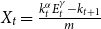 $X_t = \frac {k_{t}^{\alpha }E_{t}^{\gamma } - k_{t+1}}{m}$
. Parameter
 $\varphi$
is the fraction of taxes used for environmental improvement and thus
 $(1-\varphi )$
is used for abatement, with the respective semi-elasticities
 $\varepsilon _{I}\gt 0$
and
 $\varepsilon _{A}\lt 0$
. Finally,
 $\Omega X_t$
is the total pollution produced by brown projects that weigh on the environmental quality. Note that we do not model any accumulation or decumulation of environmental stocks over time. This assumption is consistent with our focus on short-run business-cycle dynamics and parallels the treatment of physical capital in the OLG framework, which fully depreciates each period. The natural level of the resource,
 $\bar {E}$
, defines the level of the resource if there are no brown projects at work generating emissions or taxes. Once brown project activity starts, this level decreases by total pollution
 $\Omega X_t$
. While damaging the resource, taxes accrue in the presence of a
 $\theta \gt 0$
, which then can be used twofold. First, introducing measures to improve the resource directly, e.g., by reforestation. The respective semi-elasticity
 $\varepsilon _I$
steers the effectivity of the improvement measures. As a second measure, abatement has the potential to directly diminish the emitted pollutants, as for instance filters. Again, the attached semi-elasticity,
 $\varepsilon _{A}$
, steers the ”productivity” of this abatement technology. This specification closely follows the argumentation in Brock and Taylor (Reference Brock and Taylor2010). To summarize, our specification features three avenues for regulation, with different general equilibrium and environmental effects. The environmental haircut
 $(1-\mu )$
and the Pigouvian tax
 $\theta$
represent financial and fiscal regulation, respectively, and are thus our two main policy parameters. The parameter
 $\varphi$
distributes the accrued taxes to either improve the environment directly or install abatement devices.
Remark: The environmental resource affects the economy only through production and not through households’ utility. Accordingly, agents do not internalize their environmental impact when allocating their net worth, but treat it as a pure externality. Policymakers, by contrast, are assumed to pursue multiple objectives, like higher environmental quality, higher income, lower fluctuations, and improved income distribution. We deliberately refrain from specifying an explicit policy target function, since doing so would require assigning arbitrary weights to these objectives. If policymakers act in the interest of households, then implicitly households also care about environmental quality, income, distribution, and stability, without us having to assume specific trade-offs.
4.3 Short-run equilibrium and its dynamics
We are now in a position to characterize the short-run equilibrium and derive its implied dynamics. In the short-run equilibrium
 $\rho ^{e}_{t+1}=r^{e}_{t+1}$
must hold with equality, as otherwise agents would never be willing to start brown projects due to the lower profitability compared to green projects. Hence, they will simply not be funded as the rate of return of lending is too low. This implies that
 \begin{equation} \rho _{t+1}^{e}=r^{e}_{t+1}=\frac {\partial f(k_{t+1},E_{t})}{ \partial k_{t+1}}=\frac {\alpha }{1-\alpha }k_{t+1}^{\alpha -1}E_{t}^{\gamma }\geq R(k_{t},E_{t}). \end{equation}
Now, if
 $\rho ^{e}_{t+1}=r^{e}_{t+1}\lt R(k_{t},E_{t})$
would hold with strict inequality, it is always desirable to start brown projects (higher returns). However, due to the return of lending being too low, agents will not be able to obtain credit as nobody would provide the required credit. Hence, this cannot be an equilibrium.
The short-run equilibrium value of
 $k_t$
determines the level of investment in green projects in the next period,
 $k_{t+1}$
, and thereby defines the dynamic map. We distinguish three regimes. In the first regime, when capital
 $k_t$
is low, green projects are more profitable than their brown counterparts; that is,
 $\rho ^{e}_{t+1} \gt R(k_t, E_t)$
in equation (9). Agents would never run brown projects, and capital will only flow toward green projects. This is due to the PC and the implied law of motion is
 \begin{equation} k_{t+1}=\Psi _{L}=E_{t}^{\gamma }k_{t}^{\alpha }. \end{equation}
This mechanism reflects a Solow-type accumulation process. Starting from a low level of investment in green projects, it initially increases, but rising capital reduce its profitability. At some point, green and brown projects become equally profitable, after which agents strictly prefer brown projects due to their higher returns. Now the regulatory constraint becomes binding, as the financial regulator steers the environmental haircut, making financing harder. Thus, with a net worth still too low to provide sufficient collateral, i.e., as borrowers are not able to pledge the full expected return to the lender, agents can still only start green projects and equation (10) continues to apply.
With increasing investment in green projects, the agents net worth increases. If it is sufficiently high (or the financial regulation loose enough), the RC eases. There exists a threshold,
 $k_{c}$
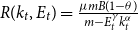
, where the regulatory constraint (see equations (4) and (9)) is satisfied with equality (and all agents still invest only in green projects). Observing that
 $R(k_{t},E_{t})=\frac {\mu mB(1-\theta )}{m-E_{t}^{\gamma }k_{t}^{\alpha }}$
and inserting equation (10) into equation (9) allows to determine the respective threshold
 $k_c$
. That is implicitly given as
 $k_{c}=\left [\frac {\alpha }{1-\alpha } \frac {1}{\mu B(1-\theta )} \left (1-\frac {k_{c}^{\alpha }E_{t}^{\gamma }}{m}\right ) E_{t}^{\alpha \gamma }\right ]^{\frac {1}{\alpha (1-\alpha )}}$
. In the second regime, the short-run value of investment in green projects is beyond this threshold, i.e.,
 $k_{t}\gt k_{c}$
, brown projects can and will be financed. The credit flow is determined such that the maximum pledgeable rate of return,
 $R(k_{t},E_{t})$
, equals the expected return on green projects, ensuring that equation (9) continues to hold with equality for
 $k_{t} \gt k_{c}$
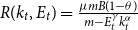
. For
 $k_{t}\lt k_{\mu }$
,
 $R(k_{t},E_{t})=\frac {\mu mB(1-\theta )}{m-E_{t}^{\gamma }k_{t}^{\alpha }}$
and the resulting dynamic equation is
 \begin{equation} k_{t+1}=\Psi _{M}=\left [\frac {\alpha }{1-\alpha } \frac {1}{\mu B(1-\theta )} \left (1-\frac {k_{t}^{\alpha }E_{t}^{\gamma }}{m}\right )\right ]^{\frac {1}{1-\alpha }} E_{t}^{\frac {\gamma }{1-\alpha }}. \end{equation}
In the third regime, either net worth is sufficiently high or regulation sufficiently loose to overcome the RC. Once capital exceeds the threshold
 $k_{\mu } = \left ( (1-\mu )mE_t \right )^{1/\alpha }$
, all additional credit flows into brown projects. Hence, investment in green projects is determined by
 $\rho ^{e}_{t+1}=\frac {\partial f(k_{t+1},\,E_{t})}{ \partial k_{t+1}}=B(1-\theta )$
such that the dynamics follow
 $\Psi _{R}$
,
 \begin{equation} k_{t+1}=\Psi _{R}=\left [\frac {\alpha }{1-\alpha } \frac {1}{B(1-\theta )}\right ]^{\frac {1}{1-\alpha }} E_{t}^{\frac {\gamma }{1-\alpha }}. \end{equation}
We are now able to specify the full dynamic equation, by putting above derivations together. The three regimes, indicated by
 $\Psi _{i},\,i\in (L,M,R)$
, are separated by the thresholds
 $k_{c}$
and
 $k_{\mu }$
.
 \begin{equation} \begin{array}{ll} k_{t+1}= & \left \{ \begin{array}{l@{\quad}ll} \Psi _{L}=k_{t}^{\alpha }E_{t}^{\gamma } & \text{if } & k_{t}\leq k_{c} \\ \Psi _{M}=\left [ \frac {A}{\mu }\left ( 1-\frac {k_{t}^{\alpha }E_{t}^{\gamma }}{m}\right ) \right ] ^{\frac {1}{1-\alpha }}E_{t}^{\frac {\gamma }{1-\alpha }} & \text{if } & k_{c}\leq k_{t}\leq k_{\mu } \\ \Psi _{R}=\left ( \frac {A}{\mu }\right ) ^{\frac {1}{1-\alpha }}E_{t}^{\frac {\gamma }{1-\alpha }} & \text{if } & k_{t}\geq k_{\mu }\end{array}\right . \\ & \\ E_{t+1}= & \ \ \ \Phi =\dfrac {\bar {E}+[\varphi \theta m BX_{t}]^{\varepsilon _{I}}}{1+\frac {1}{1+((1-\varphi )\theta m BX_{t})^{-\varepsilon _{A}}}\Omega X_{t}} \ \ \ \ \ \forall k_{t}\end{array} \end{equation}
where
 \begin{equation} X_{t}=\frac {k_{t}^{\alpha }E_{t}^{\gamma }-k_{t+1}}{m} \end{equation}
denotes the number of brown projects and
 \begin{equation} A=\frac {\alpha }{1-\alpha }\frac {1}{B(1-\theta )} \end{equation}
collects a parameter cluster for future reference.
The map is thus piecewise-smooth with the two variables
 $k_{t}$
and
 $E_{t}$
. The first and second regime are separated by
 \begin{equation} k_{c}=\left [ \frac {\alpha }{1-\alpha }\frac {1}{\mu B(1-\theta )}\left ( 1-\frac {k_{c}^{\alpha }E_{t}^{\gamma }}{m}\right ) E_{t}^{\alpha \gamma }\right ] ^{\frac {1}{\alpha (1-\alpha )}} \end{equation}
The threshold between the second and third regime is
 \begin{equation} k_{\mu }=[m(1-\mu )E_{t}^{-\gamma }]^{1/\alpha }. \end{equation}
Note that both thresholds depend on
 $E_t$
and are thus time-dependent. We restrict the twelve parameters as follows:
 $\varepsilon _{A}\lt 0$
;
 $0\lt \alpha ,\gamma ,\mu ,\varphi ,\theta \lt 1$
;
 $\Omega ,\bar {E},\varepsilon _{I}\gt 0$
and
 $m,B\gt 1$
.
Remark 1: Note that in this setup, multiple project types coexist in equilibrium because sectoral heterogeneity and financial frictions prevent any single option from dominating. Green projects generate net worth by employing the young generation, brown projects require external finance and face collateral constraints, and lending provides an alternative use of savings. These frictions and complementarities ensure that none of the options disappears completely (except in the left regime
 $\Psi _L$
, where all credit flows to green projects due to low net worth or high regulatory burden), which sustains the cyclical dynamics we analyze.
Remark 2: Note that only in the absence of an environmental sector and respective taxation (i.e., for
 $\gamma = \theta = 0$
) does the model collapse to the original framework of Matsuyama et al. (Reference Matsuyama, Sushko and Gardini2016). In that case, it reduces to a one-dimensional piecewise-smooth map in
 $k_t$
, consisting of
 $\Psi _i \ (i \in \{L, M, R\})$
as defined in equation (13). Introducing environmental dynamics, represented by
 $\Phi$
in equation (13), adds a second, interdependent dimension: environmental quality depends on the evolution of physical capital
 $k_t$
, and in turn, it affects the dynamics of physical capital. This mutual dependence increases the analytical complexity of the model, even though the underlying rationale for endogenous cycles continues to rest on the model’s core mechanism. Consequently, the results of Matsuyama et al. (Reference Matsuyama, Sushko and Gardini2016) cannot be directly applied.
4.4 Global dynamics: analytical results
This and the subsequent subsections examine the interaction between parameters and how these interactions influence the system’s dynamics and stability from both analytical and numerical perspectives. The economic interpretation and discussion are reserved for Section 5.
Depending upon the regime, the map has a unique fixed point with distinct characteristics. The following propositions outline the key properties of the fixed points in the left and in the right regime. Due to the analytical complexity, we do not provide explicit results for the fixed point in the middle regime. However, the properties of the fixed points in the left and right regimes have implications for the fixed point in the middle regime.
Proposition 1.
In the left regime, the fixed points of
 $k$
and
 $E$
is given as
 \begin{equation*} \begin{array}{lll} k_{L}^{\ast }=\Psi _{L}\left ( k_{L}^{\ast },E_{L}^{\ast }\right ) & & k_{L}^{\ast }=\left ( E_{L}^{\ast }\right ) ^{\frac {\gamma }{1-\alpha }} \\ & & X_{L}^{\ast }=0\\ E_{L}^{\ast }=\Phi \left ( X_{L}^{\ast }\right ) & & E_{L}^{\ast }=\bar {E} \end{array} \end{equation*}
Property 1:
The fixed point
 $L$
is (locally) stable for
 $\alpha \lt 1$
, which holds via assumption.
Property 2:
The fixed point
 $L$
collides with
 $k_{c}$
, given in equation (
16
) at
 \begin{equation*} \mu ^{BC-Lkc}=A\left ( 1-\frac {\bar {E}^{\frac {\gamma }{1-\alpha }}}{m}\right ). \end{equation*}
Property 3:
The fixed point
 $L$
potentially collides with
 $k_{\mu }$
as defined in (
17
) at
 \begin{equation*} \mu ^{BC-Lk\mu }=1-\frac {\bar {E}^{\frac {\gamma }{1-\alpha }}}{m}. \end{equation*}
Note that for
 $A=\frac {\alpha }{1-\alpha }\frac {1}{\left ( 1-\theta \right ) B}\lt 1$
,
 $\mu ^{BC-Lkc}\lt \mu ^{BC-Lk\mu }$
. In that range,
 $\mu ^{BC-Lkc}$
is the relevant threshold.
 $A=\frac {\alpha }{1-\alpha }\frac {1}{\left ( 1-\theta \right ) B}=1$
defines a critical value
 \begin{equation*} \theta ^{crit}=1-\frac {\alpha }{\left ( 1-\alpha \right ) B}. \end{equation*}
Proof. See Appendix A.
Proposition 2.
In the right regime, the fixed points of
 $k$
and
 $E$
are implicitly given as
 \begin{equation*} \begin{aligned} k_{R}^{\ast } &= \Psi _{R}\left ( k_{R}^{\ast }, E_{R}^{\ast } \right ) = A^{\frac {1}{1 - \alpha }} \left ( E_{R}^{\ast } \right )^{\frac {\gamma }{1 - \alpha }} \\ X_{R}^{\ast } &= \frac {1}{m} A^{\frac {\alpha }{1 - \alpha }} (1 - A) \left ( E_{R}^{\ast } \right )^{\frac {\gamma }{1 - \alpha }} \\ E_{R}^{\ast } &= \Phi \left ( X_{R}^{\ast } \right ), \end{aligned} \end{equation*}
where
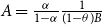 $ A = \frac {\alpha }{1 - \alpha } \frac {1}{(1 - \theta ) B}$
.
Property 1:
 $ X_{R}^{\ast } \gt 0$
for
 $ \theta \lt \theta ^{\text{crit}}$
. For
 $ \theta = \theta ^{\text{crit}}$
, we have
 $ X_{R}^{\ast } = 0$
, and the
 $ R$
fixed point collides with the
 $ L$
fixed point. For
 $ \theta \gt \theta ^{\text{crit}}$
, the
 $ R$
fixed point no longer exists.
Property 2:
The
 $ R$
fixed point collides with
 $ k_{\mu }$
at
 $ \mu ^{BC-Rk\mu }$
, which is implicitly defined by
 \begin{equation*} \left ( m\left ( 1-\mu ^{BC-Rk\mu }\right ) \right ) ^{\frac {1-\alpha }{\gamma }}A^{\frac {-\alpha }{\gamma }}=\frac {\bar {E}+\left ( \varphi \theta mB\left ( 1-\mu ^{BC-Rk\mu }\right ) \left ( 1-A\right ) \right ) ^{\epsilon _{I}}}{1+\frac {\Omega \left ( 1-\mu ^{BC-Rk\mu }\right ) \left ( 1-A\right ) }{1+\left [ \left ( 1-\varphi \right ) \theta mB\left ( 1-\mu ^{BC-Rk\mu }\right ) \left ( 1-A\right ) \right ] ^{-\epsilon _{A}}}}. \end{equation*}
Property 3:
The
 $ R$
fixed point collides with
 $ k_{c}$
at
 $ \mu ^{BC-Rkc}$
, which is implicitly defined by
 \begin{equation*} \left ( m\left ( 1-\mu ^{BC-Rkc}A^{\alpha -1}\right ) \right ) ^{\frac {1-\alpha }{\gamma }}A^{\frac {-\alpha }{\gamma }}=\frac {\bar {E}+\left ( \varphi \theta mB\left ( 1-\mu ^{BC-Rkc}A^{\alpha -1}\right ) \left ( 1-A\right ) \right ) ^{\epsilon _{I}}}{1+\frac {\Omega \left ( 1-\mu ^{BC-Rkc}A^{\alpha -1}\right ) \left ( 1-A\right ) }{1+\left [ \left ( 1-\varphi \right ) \theta mB\left ( 1-\mu ^{BC-Rkc}A^{\alpha -1}\right ) \left ( 1-A\right ) \right ] ^{-\epsilon _{A}}}}. \end{equation*}
Analogous to Proposition 1, note that
 $\mu ^{BC-Rk\mu } = \mu ^{BC-Rkc} A^{\alpha - 1}$
. For
 $A = \frac {\alpha }{(1 - \alpha )(1 - \theta ) B} \lt 1$
, it follows that
 $\mu ^{BC-Rkc} \lt \mu ^{BC-Rk\mu }$
. Hence, in this range,
 $\mu ^{BC-Rk\mu }$
constitutes the relevant threshold. Moreover, for
 $\theta = \theta ^{\text{crit}} = 1 - \frac {\alpha }{(1 - \alpha )B}$
(i.e.,
 $A = 1$
), all thresholds coincide:
 $\mu ^{BC-Rkc} = \mu ^{BC-Rk\mu } = \mu ^{BC-Lkc} = \mu ^{BC-Lk\mu } = 1 - \frac {\bar {E}^{\frac {\gamma }{1 - \alpha }}}{m}=\mu ^{crit}$
.
Proof. See Appendix A.
In Propositions 1 and 2, we derived analytic expressions for the border collision lines that partition the parameter plane. The respective fixed point exists for parameter combinations within one partition, while for parameter combinations in the other partition, the corresponding map exits its defining range (see equation (13)), and the fixed point no longer exists. Although we do not have explicit analytic results for the middle regime, these boundaries have implications for it: parameter combinations for which neither the left nor the right regime applies correspond to dynamics governed by the middle regime.
To prepare the ground for the numerical analysis, the following corollary summarizes the properties of the relevant critical lines and critical points.
Corollary 1.
It is possible to describe –almost fully– the parameter dependencies of
 $\mu ^{BC-Lkc}$
,
 $\mu ^{crit}$
, and
 $\theta ^{crit}$
. For
 $\mu ^{BC-Rk\mu }$
, however, results can only be obtained in the border case where
 $\theta = 0$
.
Property 1:
The derivative
 $\frac {d\mu ^{BC-Lkc}(\theta )}{d\theta } \gt 0$
, i.e., the slope of the border collision curve for the left fixed point is positive.
Property 2:
The derivative
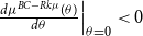 $\left .\frac {d\mu ^{BC-Rk\mu }(\theta )}{d\theta }\right |_{\theta =0} \lt 0$
, i.e., the slope of the border collision curve for the right fixed point is negative at
 $\theta = 0$
.
Property 3: In addition, the following parameter dependencies can be shown. Arrows indicate the direction of change in each threshold or critical value when the corresponding parameter increases:

Remark: Note that at the point
 $(\mu ^{\text{crit}}, \theta ^{\text{crit}})$
, the bifurcation curves
 $\mu ^{BC\text{-}Lkc}(\theta )$
and
 $\mu ^{BC\text{-}Rk\mu }(\theta )$
coincide. The corresponding results therefore apply to both curves.
Proof. See Appendix A.
4.5 Global dynamics: numerical analysis
We proceed with a numerical analysis to illustrate the analytically derived bifurcation lines and to gain further insight into the dynamics. The following parameter are set throughout the manuscript:
 \begin{equation} B = 2, m=1.05, \alpha = 0.33, \gamma = 0.4, \Omega = 1, \bar {E} = 0.8, \varepsilon _{I} = 0.5, \varepsilon _{A} = -0.5. \end{equation}
We follow the parameter specification of Matsuyama et al. (Reference Matsuyama, Sushko and Gardini2016) with respect to the exogenously given profitability of brown projects,
 $B$
, and the minimum investment size,
 $m$
. These parameters are kept constant throughout our analysis. However, as shown in Corollary 1, variations in their values would affect the results in predictable ways. The capital share is set to
 $\alpha = 0.33$
– the same value used by Matsuyama et al. (Reference Matsuyama, Sushko and Gardini2016), which is consistent with recent stylized empirical evidence (Karabarbounis, Reference Karabarbounis2024). This parameter also represents the elasticity of output with respect to physical capital. Assuming that the elasticity of output with respect to natural capital (i.e., the environmental resource) lies in a comparable range, we set
 $\gamma = 0.4$
(following Caravaggio and Sodini, Reference Caravaggio and Sodini2018). Furthermore, we normalize emissions by setting
 $\Omega = 1$
, implying proportionality between emissions and the number of brown projects. The natural environmental level,
 $\bar {E}$
, and the semi-elasticities
 $\varepsilon _{I}$
and
 $\varepsilon _{A}$
are treated as fixed constants. These parameters act primarily as scaling factors; they are not directly observable but are chosen to ensure that the key dynamic mechanisms of the model are clearly visible. As noted, Corollary 1 also indicates how variations in these parameters would influence the results.
The policy parameters – the pledgeability ratio
 $\mu$
(thus the environmental haircut
 $1-\mu$
), the environmental tax rate
 $\theta$
, and
 $\varphi$
, which governs the use of environmental tax revenues – are central to our analysis. We therefore vary them over the entire range. In particular, we consider
 $0\leq \mu , \theta \leq 0.8$
(the upper bound is set below unity because higher values no longer influence the dynamics). For
 $\varphi$
, which governs the allocation of environmental tax revenues, we primarily set
 $\varphi = 0$
, corresponding to full allocation to emissions abatement. In selected scenarios, we also consider
 $\varphi = 0.5$
, representing an equal split between abatement and environmental quality improvements. Finally, we explore the full range of allocation schemes,
 $0 \lt \varphi \lt 1$
, to highlight the non-trivial impact of tax allocation on the model’s outcomes.Footnote
7
By varying only the environmental policy parameters while keeping all other parameters fixed, we establish a consistent framework that isolates the effects of policy changes and allows us to assess their impact on the system’s dynamics.Footnote 8 This approach facilitates a clearer understanding of the interactions of financial and fiscal environmental regulation in a nonlinear dynamic general equilibrium model, where the financial market is subject to endogenous instabilities. Overall, our parameter exploration follows the approach advocated by Cai and Lontzek (Reference Cai and Lontzek2019), who caution against relying on a single calibration in climate-economic models due to inherent uncertainties. They emphasize that while optimal carbon taxation should ideally reflect the social cost of carbon, substantial variation in economic and climatic conditions leads to a wide range of plausible outcomes.
We proceed with a numerical analysis of the interaction between the two policy parameters,
 $\mu$
and
 $\theta$
, within the range
 $ 0 \leq \theta , \mu \leq 0.8$
, under the assumption that all environmental tax revenues are allocated solely to emissions abatement (i.e.,
 $\varphi = 0$
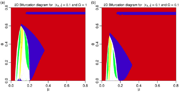
). Figure 2 presents the results: panel (a) shows a two-dimensional bifurcation diagram, while panel (b) displays the bifurcation lines corresponding to Propositions 1 and 2. In the bifurcation diagram, parameter combinations leading to convergence toward a fixed point are marked in red. In contrast, convergence to periodic cycles – specifically period-2, period-3, and period-4 cycles – is indicated in blue, yellow, and green, respectively.
The left panel (a) presents a two-dimensional bifurcation diagram in the
 $[\mu , \theta ]$
parameter plane for
 $\varphi = 0$
, illustrating the system’s stability regions and dynamic behavior. The color coding indicates convergence to different attractors: fixed point (red), period-2 cycle (blue), period-3 cycle (yellow), and period-4 cycle (green), with higher-order cycles denoted by white areas. The labels
 $\Psi _i$
(
 $i \in {L, M, R}$
) denote the regime of equation (13) in which the corresponding fixed point is located. The right panel (b) displays the bifurcation lines derived in Propositions 1 and 2, showing the boundaries between distinct dynamic regimes.

The bifurcation lines delineate three distinct regions,
 $L$
,
 $M$
, and
 $R$
, each corresponding to one of the three possible regimes where the respective fixed point exists. The middle regime is defined as the parameter region where neither the left nor the right regime applies. We have analytically shown that the left fixed point is stable. Numerical analysis further reveals that the right fixed point is also stable, while the middle fixed point loses stability at lower values of
 $\mu$
(higher values of
 $\theta$
), leading to cyclical dynamics.
We continue with a one-dimensional bifurcation analysis, presented in Figure 3, which displays bifurcation diagrams of the financial regulation parameter
 $\mu$
on
 $k_t$
for fixed values of the environmental tax rate
 $\theta$
. Specifically, the left panel (a) shows the case with
 $\theta = 0.4$
, and the right panel (b) corresponds to
 $\theta = 0.7$
, with
 $\varphi = 0$
in both cases. We use two sets of initial conditions to compute the bifurcation diagrams, shown in blue and red, respectively. The enlargement in panel (b) highlights the coexistence of a period-3 with a chaotic interval, respectively. These diagrams illustrate instances of multistability, where multiple cyclical attractors coexist within the same parameter regime. This coexistence highlights the system’s capacity for complex dynamic behavior, in which different initial conditions or slight parameter variations may lead to convergence toward distinct long-run outcomes, including periodic or potentially chaotic trajectories.
Bifurcation diagrams of the financial regulation parameter
 $\mu$
with respect to capital, for
 $\varphi = 0$
and two different values of the environmental tax rate
 $\theta$
. Panel (a) displays the case for
 $\theta = 0.4$
, while panel (b) shows the scenario for
 $\theta = 0.7$
, including an enlargement of the interval
 $\mu \in [0.16, 0.17]$
. colors indicate the two sets of initial conditions used for computation.

Finally, Figure 4 is drawn for
 $ \varphi = 0.5$
. The top left panel (a) shows a 2D bifurcation diagram, while the top right panel (b) depicts the bifurcation lines, highlighting the boundaries of different dynamical regimes. Note the small gray region, which is magnified in the bottom left panel (c). In this region, where
 $ \mu ^{BC-Rk\mu } \leq \mu \leq \mu ^{BC-Lkc}$
, both fixed points
 $ L$
and
 $ R$
coexist, indicating a parameter range with multi-stable behavior. The red/blue arrow refers to the one-dimensional bifurcation diagram in the bottom right panel (d), with
 $ \theta = 0.72$
fixed, illustrating the coexistence of attractors in this region. Using one set of initial conditions, the bifurcation diagram (shown in blue) exhibits a sharp transition from
 $k^{*}_{R}$
to
 $k^{*}_{L}$
as
 $\mu$
falls below
 $0.146$
. In contrast, when using a different set of initial conditions, the bifurcation diagram (shown in red) indicates that
 $k^{*}_{R}$
persists until
 $\mu$
declines to
 $0.113$
. For
 $\mu \lt 0.113$
, the system eventually converges to
 $k^{*}_{M}$
. Thus, for
 $ \mu ^{BC-Rk\mu }(\theta = 0.72) = 0.113 \leq \mu \leq 0.146 = \mu ^{BC-Lkc}(\theta = 0.72)$
, which corresponds to the gray region, we observe the coexistence of the fixed points
 $L$
and
 $R$
. This coexistence highlights the system’s capacity for complex behaviors, where multiple stable outcomes can arise depending on initial conditions and specific parameter values. Such findings underscore the rich dynamics and sensitivity to parameter changes present in the model, suggesting that policy measures affecting
 $ \mu$
or
 $ \theta$
could lead to unintended shifts in stability. This sensitivity implies that small adjustments in policy parameters could move the system across bifurcation thresholds, potentially triggering shifts from one stable state to another or even to cyclical behavior. These phenomena highlight the need for a cautious design of intervention strategies.
The upper left panel (a) presents a two-dimensional bifurcation diagram in the
 $[\mu , \theta ]$
parameter plane for
 $\varphi = 0.5$
, illustrating the system’s stability regions and dynamic behavior. The color coding indicates convergence to different attractors: fixed point (red), period-2 cycle (blue), period-3 cycle (yellow), and period-4 cycle (green), with higher-order cycles denoted by white areas. The labels
 $\Psi _i$
(
 $i \in {L, M, R}$
) denote the regime of equation (13) in which the corresponding fixed point is located. The upper right panel (b) displays the bifurcation lines derived in Propositions 1 and 2, showing the boundaries between distinct dynamic regimes. The lower left panel (c) provides an enlargement of the region exhibiting coexisting attractors. The red/blue line along
 $\theta = 0.72$
marks the bifurcation path illustrated in the lower right panel (d), where vertical lines denote the bifurcation values of
 $\mu$
.

5. Environmental policies and environmental quality
In this section, we provide a deeper analysis of how environmental policies impact environmental quality and explore the interactions between various policy measures. Our focus is on examining both the direct effects of individual policies and the combined effects when multiple environmental policies are implemented simultaneously.
First, an inspection of equation (13) and the two thresholds defined in equations (16) and (17) reveals that financial regulation, as represented by
 $ \mu$
, affects only the thresholds and the dynamics in the
 $ M$
regime. In this
 $ M$
regime, brown projects are initiated, but their quantity is limited by the financing constraints governed by
 $ \mu$
. Importantly,
 $ \mu$
has no impact in the
 $ L$
regime, where the marginal green project yields a higher return than a brown project, nor in the
 $ R$
regime, where brown project financing is unrestricted. As a result, the influence of
 $ \mu$
is limited to the middle
 $ M$
regime, emphasizing its effectiveness as a policy instrument only under specific conditions.
Second, tightening financial conditions for brown projects – by reducing
 $ \mu$
– can shift the economy sequentially from the
 $ R$
regime to
 $ M$
, and ultimately to
 $ L$
(as illustrated in Figures 2 and 4). In doing so, green financial regulation has the potential to phase out brown projects entirely by moving the system toward the
 $ L$
regime, where green projects dominate due to their comparatively higher returns. This transition demonstrates the policy’s ability to reshape investment dynamics by directing credit toward green projects and limiting financing for brown projects, thereby supporting an environmentally oriented economic transformation. More broadly, the analysis can be understood as a simulation of the financial sector’s green transition, in which successive regulatory measures progressively restrict brown projects’ access to credit. In our case, this mechanism is represented through the collateral eligibility of the expected returns from brown projects. More generally, however, brown assets used as collateral may also not be fully accepted, meaning that a higher amount of collateral is required relative to the credit value.
Third, it is not immediately clear whether this shift will also lead to an improvement in environmental quality, as this outcome depends on the interaction with green fiscal policy. On one hand, a reduction in brown projects lowers emissions, contributing positively to environmental goals. On the other hand, it also reduces tax revenue, which plays a crucial role in funding improvements to environmental quality. When
 $\varphi = 0$
, we obtain
 $E_{R}^{\ast } \lt E_{L}^{\ast } = \bar {E}$
. In this case, no tax revenues are devoted to environmental improvement, and only the direct emission-reduction effect is present. Consequently, for
 $\varphi = 0$
, environmental quality in the
 $R$
regime never exceeds
 $\bar {E}$
, which corresponds to the equilibrium level in the
 $L$
regime. However, when
 $\varphi$
(and
 $\theta$
) are sufficiently high, the positive effect of fiscal spending on environmental quality may dominate, leading to
 $E_{R}^{\ast } \gt E_{L}^{\ast } = \bar {E}$
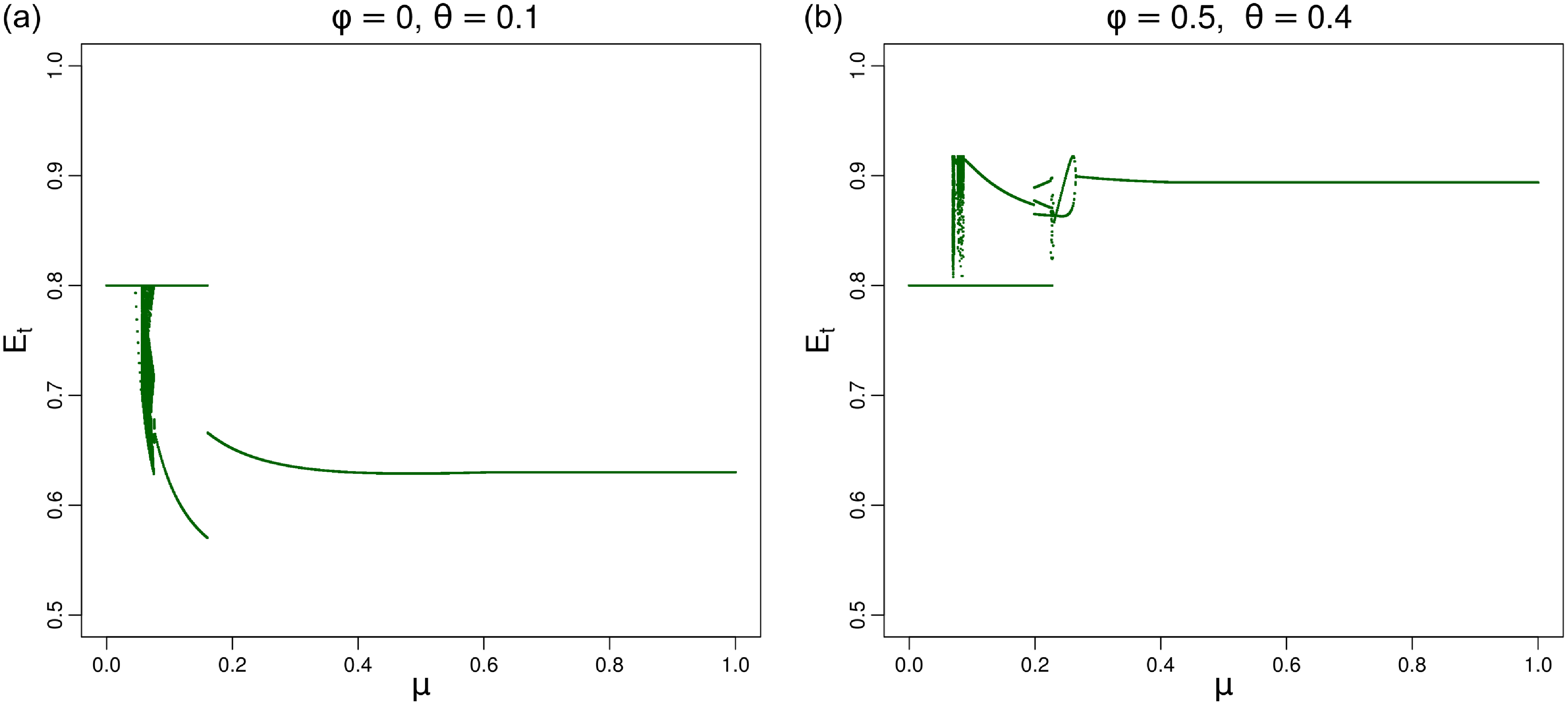
. Figure 5 illustrates this mechanism by displaying one-dimensional bifurcation diagrams for
 $0 \lt \mu \lt 0.8$
, where environmental quality is plotted on the vertical axis. For low values of
 $\mu$
, the system remains at the fixed point in the
 $L$
regime, and environmental quality equals
 $\bar {E}$
. As
 $\mu$
increases, the system transitions through the
 $M$
regime, where cyclical dynamics emerge, and eventually settles at the fixed point in the
 $R$
regime. The left panel (for
 $\varphi = 0$
) confirms that
 $E_{R}^{\ast } \lt E_{L}^{\ast } = \bar {E}$
, while the right panel (for
 $\varphi = 0.5$
) shows the opposite relationship,
 $E_{R}^{\ast } \gt E_{L}^{\ast } = \bar {E}$
, indicating that higher fiscal allocation toward environmental improvement can offset the emission effect and enhance environmental quality in the high-capital regime.
Bifurcation diagram of
 $\mu$
on the environmental quality,
 $E_t$
. In the left panel (a) parameter
 $\varphi =0$
,
 $\theta =0.1$
and in the right panel (b)
 $\varphi =0.5$
,
 $\theta =0.4$
.

Fourth, even for
 $ \varphi = 0$
, the relationship between financial regulation and environmental quality is not necessarily monotonous. Figure 6 presents a one-dimensional bifurcation diagram concerning
 $ \mu$
, with
 $ \varphi = 0$
and
 $ \theta = 0.1$
. The left panel illustrates environmental quality (in green), the middle panel shows per capita capital (in blue), and the right panel depicts the number of brown projects (in black). This diagram highlights the transition between the
 $ M$
and
 $ R$
regimes. Interestingly, reducing
 $ \mu$
initially leads to an increase in the number of brown projects, while environmental quality declines. In equilibria with lower
 $ \mu$
, financing brown projects becomes more challenging, which subsequently boosts investment in green projects, leading to an increase in the capital stock and, consequently, wages. Despite the deterioration in environmental quality, the higher wage rate enables the financing of more brown projects, even under stricter financial regulations. Initially, this latter effect dominates.
These bifurcation diagrams present the relationship between the parameter
 $\mu$
and the environmental quality in panel (a) in green, the per capita capital in panel (b) in blue, and the number of brown projects in panel (c) in black. Free parameters set to
 $\varphi = 0$
and
 $\theta = 0.1$
.

Fifth, when focusing solely on green fiscal policy and abstracting from financial frictions, we observe that a tighter fiscal stance shifts the economy from the
 $R$
regime to the
 $L$
regime (see Figures 2 and 4 for sufficiently high values of
 $ \mu$
). Figure 7 displays a one-dimensional bifurcation diagram for
 $ 0 \lt \theta \lt 0.8$
, with
 $ \mu = 0.7$
in the left panel. As before, green denotes environmental quality, blue represents capital per worker, and black indicates the number of brown projects. For
 $\varphi =0$
, depicted in the left panel (with an enlargement of brown projects in the middle panel), we find that
 $E_{R}^{\ast }\lt \bar {E}=E_{L}^{\ast }$
, which also implies that
 $k_{R}^{\ast }\lt k_{L}^{\ast }$
. Interestingly, the effect of increasing environmental taxes on the number of brown projects is non-monotonic. On the one hand, an increase in
 $\theta$
reduces the net return of brown projects and thus encourages greater investment in green projects, which also raises
 $k^{\ast }$
. On the other hand, this shift increases wages, which in turn raises the number of brown projects. Initially, the latter effect dominates, so that, counterintuitively, the number of brown projects increases with
 $\theta$
. However, for sufficiently high values of
 $\theta$
, the number of brown projects begins to decline. At first, environmental quality also improves despite the rise in the number of brown projects, since the abatement effect outweighs the additional pollution. Once the number of brown projects starts to fall, both effects reinforce each other, leading to further improvements in environmental quality. In the right panel, with
 $\varphi =0.5$
, we observe the same non-monotonic pattern for the number of brown projects. Similar to Figure 5, environmental quality in the
 $R$
regime can exceed
 $\bar {E}$
if the improvement policy is sufficiently strong, that is, when
 $\varphi$
and
 $\theta$
are both high.
Bifurcation diagram of
 $ \theta$
with
 $ \mu = 0.7$
. In panel (a)
 $ \varphi = 0$
, with an enlargement of number of brown projects,
 $X_t$
in panel (b). The right panel (c) shows
 $ \varphi = 0.5$
. In all panels, green represents the environmental quality, blue the capital per worker, and black the number of brown projects, respectively.

Sixth and finally, we examine the role of fiscal policy in allocating environmental tax revenues. In previous simulations, we focused on two specific cases: taxes allocated entirely to abatement measures (i.e.,
 $\varphi =0$
) and an even split between abatement and improvement (i.e.,
 $\varphi =0.5$
). However, our model allows us to explore the full spectrum of possible allocations. Figure 8 presents a bifurcation diagram that maps the effect of varying the allocation parameter
 $\varphi$
on both capital (in blue) and the environment (in green). This diagram reveals a crucial asymmetry: increasing
 $\varphi$
, i.e., shifting more tax revenue toward improvement measures, can elevate environmental quality beyond
 $\bar {E}=0.8$
. In contrast, abatement alone merely mitigates ongoing environmental degradation. This functional distinction between improvement and abatement helps explain the model’s dynamic behavior. In Figure 8 the system exhibits complex dynamics for low values of
 $\varphi$
. Only when
 $\varphi$
increases beyond a certain threshold does the system converge to a stable fixed point. These results suggest that the allocation of environmental tax revenues can itself become a source of macroeconomic instability if not carefully coordinated with broader fiscal and financial regulatory policies.
Bifurcation diagram of
 $ \varphi$
with
 $ \mu = 0.15$
and
 $\theta =0.72$
on capital (blue) and the environment (green).

6. Environmental policy, income and income distribution
6.1 Income definitions
Our specification allows us to analyze not only the overall income of the economy but also to differentiate income by agent types. Specifically, we distinguish between the labor income of the young generation and three categories of income for the old generation. The latter includes income from green projects, income from brown projects, and income from lending. Since we model the environmental resource as part of total factor productivity, its returns are not tied to a single income group.
We start our analysis at time
 $t+2$
, where total income comprises both labor and investment income generated by two generations. The young generation, denoted as
 $L_{t+1}$
, earns labor income
 $w_{t+1}$
from their work during period
 $t+1$
, which extends until time
 $t+2$
. The old generation, represented by
 $L_{t}$
, requires closer examination. They receive returns on investments made at point
 $t+1$
. It is important to consider the prevailing regime described in equation (13) when calculating the respective income for both generations.
First, in a situation where only green projects can be started due to tight regulation or low net worth, i.e., in regime
 $\Psi _{L}$
with
 $k_{t}\lt k_{c}$
, the income is based on the factor remunerations. Thus the income is determined by
 \begin{equation} I_{t+2}|\Psi _{L}=(\underbrace {k_{t+1}^{\alpha }E_{t+1}^{\gamma }}_{\text{wage young}})\cdot L_{t+1}+(\underbrace {\frac {\alpha }{1-\alpha }k_{t+1}^{\alpha -1}E_{t+1}^{\gamma }w_{t}}_{\text{return old (Green)}})\cdot L_{t} \end{equation}
As net worth increases (or regulation becomes looser), brown projects will be initiated, indicating that we are above the threshold
 $k_{c}$
and thus in regimes
 $\Psi _{M}$
or
 $\Psi _{R}$
. Total income now includes the labor remuneration of young agents as well as investment returns from both green and brown projects, in addition to income from lending. To allocate this income to the respective groups within the old generation
 $L_{t}$
, we must determine the generational shares of green investors,
 $L_{t}^{G}$
, brown investors,
 $L_{t}^{B}$
, and lenders,
 $L_{t}^{L}$
. In equilibrium, aggregate credit supply must equal aggregate credit demand, which can be expressed as
 $w_{t}L_{t} = k_{t+1}L_{t+1} + mL_{t}^{B}$
. Here,
 $L_{t}^{B}$
represents the number of agents investing in brown projects and thus coincides with the number of these projects. By definition, we have
 $L_{t} = L_{t+1} = 1$
, which allows us to determine
 $L_{t}^{B}$
.
The return on brown projects, after accounting for taxes, is expressed as
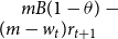 $mB(1-\theta ) - (m - w_{t})r_{t+1}$
, where lenders receive interest payments from brown investors. Consequently, green investors earn a profit rate on their invested net worth from the previous period, while brown investors accrue returns and must also cover their credit repayments. The total credit payment is given by
 $(m - w_{t})r_{t+1}L_{t}^{B}$
, with each lender receiving
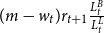 $(m - w_{t})r_{t+1} \frac {L_{t}^{B}}{L_{t}^{L}}$
from the brown investors. The return for green projects has been already defined above.
We define the lenders,
 $L_{t}^{L}$
, as the residual agents who do not engage in either green or brown projects. From this definition, we can derive the following income fractions and schedules:
 \begin{align} L_{t}^{G}=\frac {k_{t+1}L_{t+1}}{L_{t}w_{t}} &\quad\text{each with income}\quad R_{t+1}^{G}=r_{t+1}w_{t}\end{align}
 \begin{align} L_{t}^{B}=\frac {w_{t}L_{t}-k_{t+1}L_{t+1}}{m} &\quad\text{each with income}\quad R_{t+1}^{B}=mB(1-\theta )-(m-w_{t})r_{t+1}\end{align}
 \begin{align} L_{t}^{L}=L_{t}-L_{t}^{G}-L_{t}^{B} &\quad\text{each with income}\quad R_{t+1}^{L}=(m-w_{t})r_{t+1}\frac {L_{t}^{B}}{L_{t}^{L}}.\\[13pt] \nonumber\end{align}
With these derivations, the aggregated income equations for the the middle and right regimes reads
 \begin{align} I_{t+2}|\Psi _{M},\Psi _{R}=(\underbrace {k_{t+1}^{\alpha }E_{t+1}^{\gamma }}_{\text{wage young}})\cdot L_{t+1}+\underbrace {R_{t+1}^{G}\cdot L_{t}^{G}+R_{t+1}^{B}\cdot L_{t}^{B}+R_{t+1}^{L}\cdot L_{t}^{L}}_{\text{income old}}, \end{align}
which completes the income definition. Note that the taxes accrued in period
 $t$
are given by
 $mB\theta \cdot L_{t}^{B}$
. Importantly, only the old generation pays taxes; thus, in the following analysis, we will focus on their net income.
6.2 Results
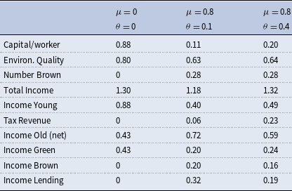
Figure 9 illustrates the one-dimensional bifurcation diagrams concerning the parameter
 $\mu$
. The parameters are set according to equation (18) with
 $\varphi =0$
. The diagrams are segmented by the values of
 $\theta$
, showcasing two distinct settings: the upper left and lower left panels correspond to
 $\theta = 0.1$
, while the upper right and lower right panels represent the scenario where
 $\theta = 0.4$
. Each panel delineates various income concepts, allowing for a comprehensive analysis of how changes in the parameter
 $\mu$
influence income dynamics within the model. The bifurcation structure provides insights into the stability of income distributions and highlights potential transitions between different economic states under varying regulatory conditions.
Bifurcation diagrams of the financial regulation parameter
 $\mu$
(horizontal axis) on average total income and average environmental quality (upper panels) and the generational incomes as well as the tax revenue (lower panels). Two distinct parameter settings (with
 $\varphi = 0$
) are presented. In the left panels (a)
 $\theta = 0.1$
, while
 $\theta = 0.4$
in the right panels (b).

Starting with
 $\theta = 0.4$
, the top right panel of the figure illustrates that tightening financial conditions, achieved by reducing
 $\mu$
, leads to an increase in average environmental quality, as previously discussed. However, the relationship between environmental quality and average income is non-monotonic. Initially, as financial restrictions take effect and the system transitions into the
 $M$
regime, income begins to rise. This increase continues until it reaches a peak, after which income declines. Notably, in the
 $L$
regime, characterized by the absence of brown projects, income falls to a level that is lower than that observed in the
 $R$
regime. This dynamic highlights a significant trade-off between environmental quality and income generation, suggesting the emergence of a potential policy dilemma. Policymakers face the challenge of promoting environmental improvements without negatively impacting income levels, highlighting the careful balance required in designing effective economic and environmental policies.
The bottom right panel illustrates the impact on income distribution. First, it is important to note that the fluctuations caused by financial market regulations are less pronounced for the income of the young generation, which derives its earnings solely from working in green projects that are not directly influenced by these regulations. Note that stricter regulations dampen the fluctuations. Second, tightening financial market regulations, by reducing
 $\mu$
, leads to a reversal in income distribution: at high values of
 $\mu$
, the net income of the old generation surpasses that of the young, while at lower values of
 $\mu$
, this relationship is reversed. The old generation loses income, while the young generation gains. These findings suggest that while stricter financial regulations may enhance environmental quality, they could inadvertently flip income disparities between generations. Policymakers should consider support measures or transfers for less well-off generations to mitigate these disparities.
We now focus on the scenario where
 $\theta = 0.1$
for comparison. The panels on the left reveal similar patterns to those seen in the previous analysis; however, a notable difference emerges: in this case, reducing
 $\mu$
leads to an increase in income within the
 $L$
regime, as illustrated in the top left panel. In this context, coordinated policy efforts could enhance the overall stability of the system, suggesting that aligning financial and environmental policies may yield beneficial outcomes for income stability and environmental quality.
As the impact of financial regulation is tied to the tax policy, a more in-depth examination of this relationship is warranted. In Table 1, we present an analysis of simulated values for key economic and environmental variables, highlighting the effects of various parameter settings, specifically for
 $\mu = 0$
,
 $\mu = 0.8$
, and two scenarios for
 $\theta$
at
 $0.1$
and
 $0.4$
. In the case where
 $\mu = 0$
, the system operates within the
 $L$
-regime, where financial decisions remain unaffected by tax policies. However, as
 $\mu$
is increased, which reflects a loosening of financial restrictions, the system transitions through the
 $M$
-regime and ultimately reaches the
 $R$
-regime, where financial constraints become negligible. This shift leads to an increase in the number of brown projects. Notably, in a higher tax environment, coupled with more stringent abatement measures, the deterioration of environmental quality is mitigated compared to the low tax regime. This enhanced environmental quality not only supports higher wage income and overall wealth but also serves as a foundation for investments by the older generation.
Simulated values for key variables across different parameter settings (with
 $\varphi =0)$
. The values are presented for
 $\mu = 0$
, indicating a scenario where no brown projects can be started, and for
 $\mu = 0.8$
, with two different values of
 $\theta$
:
 $0.1$
and
 $0.4$
. Each column corresponds to the impact of these parameters on capital per worker, environmental quality, the number of brown projects, total income, and the distribution of income among different generations

Consequently, this increased wealth enables a greater capital stock per worker, as well as a rise in the number of brown projects, even if the returns are lower due to taxation compared to the low tax regime. As a result, total income experiences an increase. In this high tax scenario, the income for the young generation rises, while the net income for the older generation declines, with green projects playing a more significant role in augmenting the income of the young. Additionally, it is important to note that income derived from lending significantly decreases; this reduction occurs because the heightened capital per worker results in lower profit rates, thereby diminishing the returns from lending activities.
7. Concluding remarks
In this paper, we analyze the interplay between fiscal and financial environmental regulation in an OLG credit cycle model, where cycles emerge endogenously. Focusing on short-run business cycles and two regulatory instruments that target brown projects, financial regulation through environmental haircuts and fiscal regulation via pollution taxes, we show how these policies jointly shape environmental quality, macroeconomic stability, and income distribution.
Our analysis shows that financial regulation plays a crucial role in shaping the composition of investment and, in turn, the stability of the economy. We find that collateral constraints and regulatory policies targeted at brown projects influence not only the distribution of credit but also the cyclicality of wages, investment, and environmental outcomes. Fiscal policies, such as taxation of brown activities, complement financial regulation by shifting incentives toward sustainable investment. We also show that the allocation of tax revenues can itself become a source of macroeconomic instability if not carefully coordinated with broader fiscal and financial policies. Taken together, our results highlight the importance of aligning financial and environmental regulation when addressing cyclical instability and environmental degradation. In particular, we find that combining financial regulation with green tax policies enhances policy effectiveness, reducing economic volatility and fostering higher income and capital accumulation. At the same time, these policies alter income distribution: younger generations and green investors benefit, while older generations that rely more heavily on capital income may be adversely affected.
We acknowledge that our framework is intentionally stylized and deliberately abstracts from growth considerations; it does not feature capital accumulation, population growth, or long-run environmental dynamics. While these aspects are interesting and relevant, analyzing them would require a different modeling framework, which we leave for future research. Further extensions could allow environmental quality to enter households’ preferences directly or provide fiscal policymakers with a third option: transferring accrued tax revenues to the worse-off generation. Such extensions would enable a deeper exploration of the effects of redistributive measures on both income distribution and the overall effectiveness of environmental policies. The environmental sector could also be refined so that abatement and improvement measures operate through distinct channels. The present paper, however, focuses on short-term business cycle fluctuations and provides a tractable setting that isolates the mechanisms through which financial frictions and environmental externalities interact. While these extensions would enrich the analysis, they would come at the cost of reduced tractability.
Acknowledgements
We thank Ana Abeliansky, Marwil Dávila-Fernández, Gilberto Lima, and three anonymous reviewers for helpful suggestions and valuable comments. We gratefully acknowledge helpful comments from the participants of the DISEI-Workshop on Climate Change and Ecological Behavior (2022, Florence), the Nonlinear Economic Dynamics Conference (2023, Kristiansand), the Macroeconomic Green Dynamics Workshop (2024, Urbino), the 12th Workshop of Dynamic Models in Economics and Finance (2024, Urbino), the MACRO-HET Workshop (2024, Siena), and the Wifo Workshop of the Vienna Climate Finance Network (2025, Vienna). Karen Spisso and Frane Gudelj provided excellent research assistance. The usual caveat applies.
Disclaimer
The views in this paper are those of the authors and do not necessarily reflect the views of the Oesterreichische Nationalbank or the Eurosystem.
Appendix A: Proofs of the Propositions
Proof of Proposition 1
In the
 $ L$
regime, note that
 $ X_{t} = 0$
(see equations (13) and (14)). Thus, the map is one dimensional
 $k_{t+1}=\Psi _{L}=\bar {E}^{\gamma }k_{t}^{\alpha }$
and
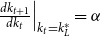 $\left . \frac {dk_{t+1}}{dk_{t}}\right \vert _{k_{t}=k_{L}^{\ast }}=\alpha$
. To derive
 $ \mu ^{BC-Lkc}$
, use equation (16), substitute
 $ k_{L}^{\ast }$
and
 $ E_{L}^{\ast }$
, and rearrange the terms. For
 $ \mu ^{BC-Lk\mu }$
, use equation (17), substitute
 $ k_{L}^{\ast }$
and
 $ E_{L}^{\ast }$
, and rearrange accordingly.
 $\blacksquare$
Proof of Proposition 2
In the
 $ R$
regime, we have
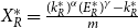 $X_{R}^{\ast } = \frac {(k_{R}^{\ast })^{\alpha } (E_{R}^{\ast })^{\gamma } - k_{R}^{\ast }}{m}$
. Using the expression for
 $ k_{R}^{\ast }$
provided in the proposition above, we simplify to obtain
 $ X_{R}^{\ast } = \frac {1}{m} A^{\frac {\alpha }{1-\alpha }} (1-A) (E_{R}^{\ast })^{\frac {\gamma }{1-\alpha }}$
. Next, consider the conditions under which
 $ X_{R}^{\ast } \gt 0$
. Specifically, we find that
 $ X_{R}^{\ast } \gt 0$
when
 $\frac {1 - \alpha }{\alpha } B(1 - \theta ) \gt 1$
, which implies
 $\theta \lt \theta ^{\text{crit}}$
. At the point where
 $\frac {1 - \alpha }{\alpha } B(1 - \theta ) = 1$
, we have
 $ X_{R}^{\ast } = 0$
, indicating that the
 $ R$
fixed point collides with the
 $ L$
fixed point. Conversely, for
 $\frac {1 - \alpha }{\alpha } B(1 - \theta ) \lt 1$
, it follows that
 $ X_{R}^{\ast } \lt 0$
, meaning the
 $ R$
fixed point ceases to exist. To derive
 $ \mu ^{BC-Rk\mu }$
, we utilize the definition provided in equation (17). Substituting in the expression for
 $ k_{R}^{\ast }$
from the proposition, we solve for
 $E_{R}^{\ast BC-Rk\mu } = (1 - \mu )^{\frac {1 - \alpha }{\gamma }} m^{\frac {1 - \alpha }{\gamma }} A^{\frac {-\alpha }{\gamma }}$
. Inserting this into
 $ X_{R}^{\ast }$
, we find
 $X_{R}^{\ast BC-Rk\mu } = (1 - \mu )(1 - A)$
. Substituting both results into
 $E_{R}^{\ast } = \Phi (X_{R}^{\ast })$
, gives us the implicit definition of
 $ \mu ^{BC-Rk\mu }$
.
For the derivation of
 $ \mu ^{BC-Rkc}$
, we reference the definition in equation (16) and insert the expression for
 $ k_{R}^{\ast }$
. Solving yields
 $E_{R}^{\ast BC-Rkc} = (1 - \mu A^{\alpha - 1})^{\frac {1 - \alpha }{\gamma }} m^{\frac {1 - \alpha }{\gamma }} A^{\frac {-\alpha }{\gamma }}$
. Inserting this into
 $ X_{R}^{\ast }$
provides
 $X_{R}^{\ast BC-Rkc} = (1 - \mu A^{\alpha - 1})(1 - A)$
. Finally, substituting both findings into
 $E_{R}^{\ast } = \Phi (X_{R}^{\ast })$
results in the implicit definition of
 $ \mu ^{BC-Rkc}$
.
 $\blacksquare$
Proof of Corollary 1
The following expressions allow us to directly assess the slope of
 $\mu ^{BC-Lkc}(\theta )$
(Property 1) and the parameter dependencies summarized in the corollary table (Property 3):
 \begin{equation*} \mu ^{BC-Lkc}(\theta ) = A \left ( 1 - \frac {\bar {E}^{\frac {\gamma }{1-\alpha }}}{m} \right ) = \frac {\alpha }{1-\alpha } \frac {1}{(1-\theta ) B} \left ( 1 - \frac {\bar {E}^{\frac {\gamma }{1-\alpha }}}{m} \right ), \end{equation*}
 \begin{equation*} \mu ^{crit} = 1 - \frac {\bar {E}^{\frac {\gamma }{1-\alpha }}}{m} \quad \text{and} \quad \theta ^{crit} = 1 - \frac {\alpha }{(1-\alpha ) B} = 1 - \frac {1}{\left ( \frac {1}{\alpha } - 1 \right ) B}, \end{equation*}
 \begin{equation*} \mu ^{BC-Rk\mu }(\theta = 0) = 1 - \frac {\bar {E}^{\frac {\gamma }{1-\alpha }}}{m} \left ( \frac {\alpha }{(1-\alpha ) B} \right )^{\frac {\alpha }{1-\alpha }}. \end{equation*}
For determining the slope of
 $\mu ^{BC-Rk\mu }(\theta )$
at
 $\theta = 0$
(Property 2), rewrite the equation in Proposition 2, Property 2 as
 \begin{equation*} \left ( m \left ( 1 - \mu ^{BC-Rk\mu } \right ) \right )^{\frac {1-\alpha }{\gamma }} A(\theta )^{\frac {-\alpha }{\gamma }} = \frac {\bar {E} + T_2(\text{tax})}{1 + T_1(\text{tax}) \, \Omega \, X(\mu ^{BC-Rk\mu }, \theta )}. \end{equation*}
Recall the definition
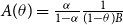 $A(\theta ) = \frac {\alpha }{1-\alpha } \frac {1}{(1-\theta ) B}$
. We assume that
 \begin{equation*} T_1(\text{tax}=0) = 1, \quad \frac {dT_1(\text{tax})}{d(\text{tax})} \lt 0, \quad T_2(\text{tax}=0) = 0, \quad \frac {dT_2(\text{tax})}{d(\text{tax})} \gt 0, \end{equation*}
with
 $\text{tax}(\theta , X) = \theta m B X$
. As shown in Proposition 2, at the border,
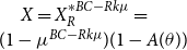 $X = X_R^{\ast BC-Rk\mu } = (1 - \mu ^{BC-Rk\mu }) (1 - A(\theta ))$
. Implicit differentiation with respect to
 $\mu ^{BC-Rk\mu }$
and
 $\theta$
then yields
 \begin{equation*} \left . \frac {d\mu ^{BC-Rk\mu }(\theta )}{d\theta } \right |_{\theta =0} \lt 0. \end{equation*}
Note that the specifications used in the main body of the paper,
 \begin{equation*} T_1(\text{tax}) = \frac {1}{1 + \left [(1-\varphi )\,\text{tax}\right ]^{-\epsilon _A}}, \quad T_2(\text{tax}) = (\varphi \cdot \text{tax})^{\epsilon _I}, \end{equation*}
satisfy the above assumptions as a special case. The proof, however, holds for the general specification.
 $\blacksquare$
Appendix B: Sensitivity Analysis
While a conventional robustness and sensitivity check is of limited use in our type of framework, where instability and sensitivity to parameter and initial condition changes are intrinsic features, we nevertheless provide some additional results with respect to the environmental dimension. As our setup is a business cycle model rather than a growth model, the length of each period can reasonably be considered shorter than in standard growth frameworks or infinite-horizon business cycle models, though we do not take a strong stance on the exact calibration of cycle length.
To account for this, we revisit our main result in Figure 4 under an alternative parametrization of the semi-elasticities of environmental quality with respect to abatement and improvement measures. Specifically, we set
 $|\varepsilon _A, \varepsilon _I|=0.1$
. Smaller absolute values of these parameters imply that both abatement and improvement exert even weaker effects on environmental quality within a single period compared to out benchmark specification. Moreover, we check for changes due to a lower negative external effect on the environment, that is, we set down
 $\Omega =0.1$
. This exercise allows us to assess whether our main findings remain valid under more conservative assumptions about the short-run effectiveness of environmental policy.
The result of this exercise is depicted in Figure B1, where in the left panel (a) we use the benchmark value
 $\Omega =1$
for the negative external effect on the environment and in panel (b) an even smaller value of
 $\Omega =0.1.$
Both panels present a two-dimensional bifurcation diagram in the
 $[\mu , \theta ]$
parameter plane for
 $\varphi = 0.5$
,
 $|\varepsilon _A, \varepsilon _I| = 0.1$
. In panel (a), the pollution parameter
 $\Omega$
is set to the benchmark value of
 $1$
, whereas in panel (b),
 $\Omega = 0.1$
, representing a scenario with even lower negative external effect on the environment. The color coding indicates convergence to different attractors: fixed point (red), period-2 cycle (blue), period-3 cycle (yellow), and period-4 cycle (green), with higher-order cycles denoted by white areas.

In our main specification (Figure 4), the stable fixed-point region dominates the parameter space, covering the majority of the
 $(\mu ,\theta )$
plane. Nevertheless, a significant region reveals periodic and chaotic dynamics, providing a clear structure of dynamical regimes. When
 $|\varepsilon _{A,I}|$
is reduced to
 $0.1$
, the proportion of stable fixed-point dynamics decreases only marginally and the periodic domain shrinks slightly, while the chaotic/irregular regions are larger. With a reduction to
 $\Omega = 0.1$
, the stabilizing effect is somewhat stronger, as the higher-order cyclical region shrinks even further and the periodic domain shifts toward lower values of
 $\mu$
and
 $\theta$
. Interestingly, the horizontal area of a period-2 cycle (in blue) along higher
 $\theta$
-values, is much more pronounced. However, we conclude that the overall qualitative picture remains very close to the benchmark.
Qualitatively, this analysis indicates that the sensitivity to
 $|\varepsilon _{A,I}|$
and
 $\Omega$
is not pronounced, especially for less strong environmental dynamics. Thus, while lower values of
 $\Omega$
, i.e., less severe negative environmental externalities, promote slightly more stability, the benchmark case captures the essential bifurcation structure reliably and remains a valid reference for system behavior.