1. Introduction
As a wearable intelligent device that integrates robotics, biomechanics, and sports science, the knee exoskeleton is progressively transitioning from laboratory research to real-world applications. It has emerged as a pivotal technological solution to tackle health challenges in an aging society and improve human locomotor capabilities [Reference Chen, Zi, Wang, Qin and Liao1]. Against the backdrop of accelerating global population aging, the prevalence of conditions such as knee osteoarthritis (KOA) and muscle strength decline has risen markedly, underscoring the pressing need for effective rehabilitation and therapeutic interventions. Epidemiology shows that the global prevalence rate of KOA is 16% for those over 15 years old and 22.9% for those over 40 years old [Reference Sampath, Venkatesan, Ghosh and Kotikalapudi2], and this serious disease has brought enormous physical and mental pain to countless patients and affected their ability to live independently [Reference March, Cross, Lo, Arden, Gates, Leyland, Hawker, King and Leyland3].
While traditional rehabilitation methods—such as physical therapy and pharmacological interventions—can alleviate symptoms, they often fail to deliver precise biomechanical support or personalized treatment. Surgical options like total knee arthroplasty are limited to severe KOA cases and carry inherent risks of complications. For mild to moderate KOA patients, wearable devices enabling conservative management and deceleration of degenerative progression have become a preferred therapeutic strategy [Reference Budarick, MacKeil, Fitzgerald and Cowper-Smith4]. In this context, knee exoskeleton technology has emerged as a research focus in rehabilitation medicine and assistive geriatric technologies, owing to its capabilities in programmable mechanical assistance, motion augmentation, and real-time biofeedback. Furthermore, in high-intensity scenarios such as military operations and industrial logistics, exoskeletons are increasingly utilized to reduce physical strain and enhance operational efficiency. To address the daily activity needs of the elderly population, research on rehabilitation and assistive knee exoskeletons has prioritized core objectives such as lightweight and portable design, safety and comfort, and functionality and intelligence. These devices are designed to support common daily activities, including walking assistance, stair climbing, and sit-to-stand transitions, aiming to reduce joint loads and slow degenerative progression through biomechanical intervention.
In terms of lightweight and portability design, existing research mainly adopts methods such as material innovation, topological optimization design [Reference Balser, Desai, Ekizoglou and Bai5–Reference Sha, Lin, Zhao and Kuang7], and the transformation of rigid exoskeletons into flexible exoskeletons [Reference Pérez Vidal, Morales, Torres, Sorcia Vázquez, Rojas, Mendoza and Rodríguez Cerda8] to design lightweight exoskeleton structures, so as to meet the movement requirements of the human body. Exoskeleton designs based on flexible materials have also been applied in lightweight design. For instance, Koo [Reference Koo, Yun, Costa, Scognamiglio, Yangali, Park and Cho9] designs and fabricates an exoskeleton-type assistive device. The exoskeleton is designed with soft materials such as fabric, rubber, wire, and other compliant materials. By adopting these materials and concentrating on specific target motions, the number and size of the actuators can be reduced, thereby decreasing the total complexity, weight, and size of the device. One of the purposes of lightweight design is to reduce the weight of the exoskeleton, thereby decreasing the load and pressure on the human body and enhancing its portability. For active exoskeletons, the portability can also be improved by changing the driving form of the exoskeleton. Take the cable-driven form as an example [Reference Tricomi, Lotti, Missiroli, Zhang, Xiloyannis, Muller, Crea, Papp, Krzywinski, Vitiello and Masia10]. In this form, the direct-drive motors at the exoskeleton joints are replaced by distal cable-driven motors, and components with a relatively large weight in the exoskeleton system, such as motors and power supplies, are placed in a backpack to reduce the weight and inertia on the user’s limbs [Reference Asbeck, De Rossi, Holt and Walsh11]. Another common driving form of exoskeletons is pneumatic drive [Reference Zhou, Hohimer, Young, McCann, Pont-Esteban, Civici, Jin, Murphy, Wagner, Cole, Phipps, Cho, Bertacchi, Pignataro, Proietti and Walsh12, Reference Veale, Staman and van der Kooij13], especially in some wearable soft exosuits. Such wearable devices offer better wearing comfort and safety compared to rigid exoskeletons. However, problems like the portability of the air source (e.g., air compressors), high noise, and the hysteresis of air inflation and deflation in the pneumatic drive form still remain to be further explored.
The Bowden cable-driven mechanism has gained increasing popularity in exoskeleton applications. Its ability to separate the driving device from the actuating components enables exoskeletons to achieve a compact structure. This spatial decoupling optimizes mechanical layout, enhances portability, and improves overall functionality. In order to improve the control accuracy of force/position in human-exoskeleton interaction, Li et al. [Reference Li, Ma and Wang14] constructed a friction model of force transmission for Bowden cables and fabrics, which serves as the basis for the compensation of the system’s force transmission. Hofmann [Reference Hofmann, Butzer, Lambercy and Gassert15] designed and evaluated a remote driving system based on Bowden cables. The integrated bending angle sensor and feedforward friction compensation model in this system can enhance the power-to-weight ratio and power-to-volume ratio of the driving system. Aiming at the inherent friction and hysteresis phenomena in cable-driven systems, Tan [Reference Tan, Shi, Mei, Geng and Yang16] proposed a novel control method. By introducing an angle recognition model, real-time detection and compensation of the cable bending angle were achieved, thus improving the force control accuracy of the cable-driven system. By imitating the activation pattern of human muscles, Xu et al. [Reference Xu, Zhou, Wang, Ruan, Mai and Wang17] proposed a bionic cable-driven design that can provide concentric and eccentric contractions and demonstrated its assisting performance in the application of an ankle exoskeleton.
The safety and comfort of exoskeletons are comprehensive issues that involve multiple aspects, such as the mechanical design, structural optimization [Reference Yang, Yin, Qi, Li, Zhou, Liu and Xu18], driving mode, and human–machine interaction algorithms of the exoskeleton [Reference Nasr, Inkol and McPhee19, Reference Nazari, Mohajer, Nahavandi, Khosravi and Nahavandi20]. Among them, the primary issue is the mechanical design of the exoskeleton [Reference Li, Liang, Lu, Su and Hou21]. The human-exoskeleton (H-E) kinematic compatibility is one of the key problems in the mechanical design of the exoskeleton. The fixed-axis design of traditional exoskeletons is prone to causing misalignment of joint axes, which can lead to discomfort for the wearer and an increase in the user’s metabolic consumption [Reference Cempini, De Rossi, Lenzi, Vitiello and Carrozza22].
Yang et al. [Reference Yang, Guo, Wang, Wu, Niu and Liu23] proposed an adaptive knee exoskeleton based on a gear-link mechanism, reducing the difficulty of aligning the H-E joint axis in the sagittal plane. Li et al. [Reference Li, Liang, Lu, Su and Hou21] proposed a self-aligning knee exoskeleton aiming to enhance wearing comfort. This exoskeleton has the ability to assist both the flexion and extension of the knee joint and the internal and external rotation of the hip joint simultaneously. Compared with existing exoskeletons, it exhibits lower H-E interaction forces and torques. Moreover, due to the characteristic of the dynamic change of the instantaneous center of rotation (ICR) of the knee joint [Reference Lee and Guo24, Reference Williams and Logan25], anthropomorphic designs [Reference Zhou, Shao, Shi, Feng, Ding and Zhang26] have been widely explored. For instance, exoskeleton joints based on cam structures mimicking the human knee have been extensively studied. The core of the cam mechanism design lies in capturing the physiological movements of the human knee joint. In this regard, Wang et al. [Reference Wang, Lee, Guo and Yang27] and Kim et al. [Reference Kim, Jeong and Kong28] successively proposed knee exoskeletons based on cam mechanisms. By analyzing the characteristics of relative rolling and sliding between the femur and the tibia, Li et al. [Reference Li, Sui, Ju, An, Zhao and Zhu29] proposed a rolling pair based on a cam structure. The exoskeleton knee joint with this structure can generate an ideal ICR curve for the knee joint, thus maintaining consistency with the rotation center of the human knee joint. In addition, a slider with an elastic limiter [Reference Liu, Han, Han and Zhang30] inspired by the knee ligaments, as well as a knee exoskeleton based on a parallel elastic self-aligning mechanism [Reference Zhang, Zhu, Song, Bao, Su, Xu, Zheng, Shi, Zhang and Li31], has also been utilized to reduce misalignment. Introducing redundant joints or designing multi-link mechanisms is also a way to improve H-E kinematic compatibility [Reference Cao, Wang, Zhang, Li and Zhang32]. However, the introduction of redundant joints [Reference Stienen, Hekman, van der Helm and van der Kooij33, Reference Choi, Lee, Kim, Lee, Lee, Roh, Choi, Kim and Choi34] and multi-link mechanisms [Reference Yang, Guo, Wang, Wu, Niu and Liu23, Reference Amigo, Casals and Amat35] will complicate the mechanical design and motion control of the exoskeleton. How to balance H-E kinematic compatibility and the complexity of the exoskeleton structure is one of the core contradictions that need to be resolved in exoskeleton design.
According to the different functions or tasks they undertake, knee exoskeletons can be classified into assistive types and rehabilitative types. Among them, the assistive knee exoskeleton is dedicated to providing torque for the knee joint to assist in the flexion and extension movements of the knee joint, and the assisting performance of the exoskeleton is evaluated through changes in muscle activities and metabolic consumption. Wu et al. [Reference Wu, Zhu, Dang and Shi36] tested the performance of a knee-ankle exoskeleton under real-world conditions. Compared with walking without an exoskeleton, when walking with the exoskeleton, the exoskeleton can reduce the energy consumption by 8.9%
 $\pm$
1.3%. Lee et al. [Reference Lee, Lee and Young37] proposed a general exoskeleton system driven by artificial intelligence. Meanwhile, Molinaro et al. [Reference Molinaro, Scherpereel, Schonhaut, Evangelopoulos, Shepherd and Young38] also proposed a task-agnostic exoskeleton control method. By estimating the joint torque through a neural network and providing assistance for the knee joint and hip joint, this system can dynamically switch the type of assistance under different walking modes, enabling it to adapt to various unstructured terrains in the real world. Compared with traditional assistance methods, the artificial intelligence-based assistance method can further reduce the metabolic cost. The reduction in metabolic cost means that the exoskeleton can help individuals improve their athletic performance. Therefore, it is suitable for people who intend to enhance their own athletic ability to help them complete a certain task more efficiently.
For knee exoskeletons used in rehabilitation and elderly care, the core technology of such exoskeletons lies in the function of intervening in the internal load of the joint while assisting the rotation of the biological knee joint. For example, actively supporting the knee joint through the exoskeleton to achieve joint unloading, so as to protect the knee joint, reduce the pressure on the user’s knee joint, and relieve pain. Typical cases are the walking assistance gravity-support system developed by Honda [Reference Ikeuchi, Ashihara, Hiki, Kudoh and Noda39] and the force-sharing device named Moon walker [Reference Krut, Benoit, Dombre and Pierrot40]. Their common feature is to provide support at the pelvis and reduce the weight-bearing of the lower limbs by exerting a vertically upward force. Similarly, a passive unloading exoskeleton [Reference Wang, Lee and Ji41] for body weight support also provides support under the pelvis and realizes the support of body weight based on the gait changes of the human body. Rodrigues et al. [Reference Rodrigues and Gonçalves42] proposed an active body weight support system for the gait rehabilitation of stroke patients. This system integrates specialized games simultaneously to enhance the rehabilitation effect and patient compliance. Regarding the use of exoskeletons to assist patients with KOA in their mobility, a study conducted in both clinical and home environments [Reference Dereshgİ, GÖSe, DemİR and Ghannam43] indicated that exoskeletons have shown improvements in cumulative effects, such as in indicators like stair test time, pain level, and functionality. Although exoskeletons have great potential in medical, industrial, and military fields, there is currently a lack of recognized performance evaluation criteria. A comprehensive study on exoskeleton performance evaluation [Reference Zhang, Chen, Huo, Liu, Zhu, Zu, Wang, Chen and Sun44] found that exoskeletons have a certain assisting effect in preliminary and semi-realistic tests, but they have deficiencies in real-world tests. This suggests that formulating a more comprehensive evaluation system can better reflect the impact of exoskeletons on the human body in the real world, or these evaluation indicators can be used to further clarify the directions for exoskeleton improvement.
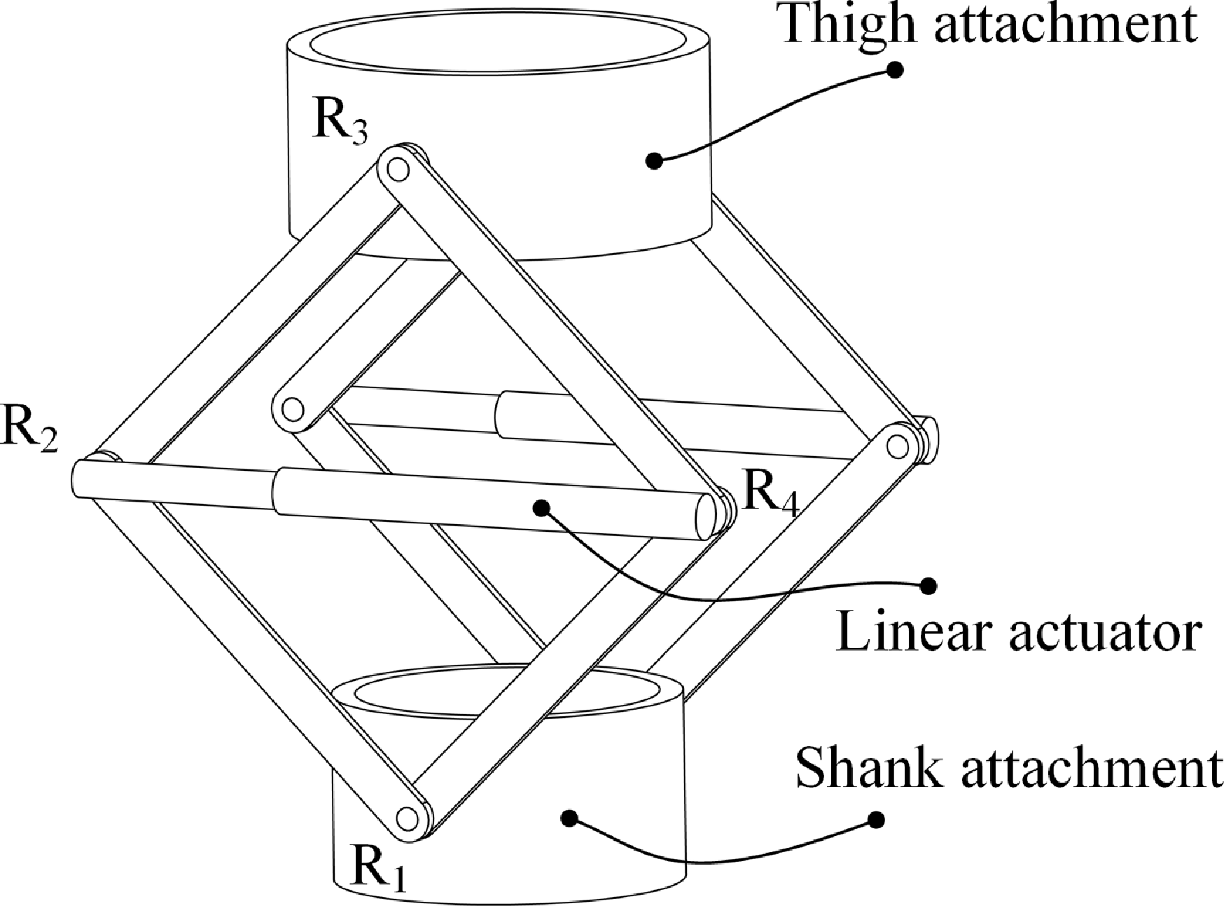
Rhombus linkage exoskeleton mechanism.

This study focuses on the mechanical design, analysis, and modeling of a novel knee exoskeleton, with the aim of providing an exoskeleton that can adapt to knee joint motion and actively support and unload the knee joint. The content of this paper is organized as follows: Section 2 introduces the exoskeleton mechanism and analyzes its degrees of freedom (DOF). Section 3 presents the kinematic modeling of the exoskeleton mechanism and the H-E closed-loop mechanism. In Section 4, the mechanical modeling of the exoskeleton driving system is conducted. Subsequently, in Section 5, the exoskeleton Bowden cable system is simulated to analyze its output characteristics. In Section 6, compatibility tests, Bowden cable output force optimization, and gait experiments were conducted, respectively, and the experimental results were discussed in Section 7. Finally, in Section 8, a summary of this paper is provided.
2. Knee exoskeleton mechanism
2.1. Exoskeleton robot structure
The design of a knee unloading exoskeleton mechanism must consider not only the physical interaction forces between the exoskeleton and the human body, specifically, the supportive forces exerted on the body, but also the kinematic characteristics of the knee joint and the H-E kinematic compatibility. The primary motion of the knee joint is flexion–extension in the sagittal plane, with a time-varying ICR. To address this, an adaptive knee mechanism for the knee unloading exoskeleton has been proposed, as illustrated in Figure 1.
The exoskeleton mechanism consists of a thigh attachment, a shank attachment, linkage rods, and a linear actuator. The thigh and shank attachments are securely attached to the thigh and shank, respectively. On both the left and right sides of the attachments, four linkage rods are connected to form a rhombus configuration, with all components joined by revolute joints (denote it with the symbol R). A linear actuator reduces the distance between the two central revolute joints (R
 $_2$
and R
 $_4$
), causing the vertical distance between the upper and lower revolute joints (R
 $_3$
and R
 $_1$
) to increase, thereby achieving active support motion. When the linear actuator is inactive, the entire mechanism passively follows the knee joint’s motion, enabling adaptive knee motion.
2.2. DOF of the exoskeleton mechanism
The knee exoskeleton mechanism, composed of linkage rods and a linear actuator, forms a multi-loop coupled parallel structure. The linear actuator is modeled as an equivalent prismatic joint (denote it with the symbol P). As shown in Figure 2, the shank attachment is designated as the fixed platform, while the thigh attachment serves as the moving platform. Fixed and moving coordinate systems are established accordingly. The origin of the fixed coordinate system, denoted as
 $O$
, is located at the center of the revolute joint R
 $_1$
. The
 $X$
-axis aligns with the axis of R
 $_1$
, the
 $Z$
-axis is oriented vertically upward, and the
 $Y$
-axis follows the right-hand rule, forming the fixed coordinate system
 $O-XYZ$
. Similarly, the origin of the moving coordinate system, denoted as
 $P$
, is positioned at the center of the revolute joint R
 $_3$
. The axes of the moving coordinate system
 $P-xyz$
are aligned with those of
 $O-XYZ$
.
Diagram of the mechanism coordinate system and screw system. (a) Mechanism coordinate system. (b) Twists and wrenches of the branch R
 $_1$
R
 $_2$
R
 $_3$
.

H-E motion matching requires that the exoskeleton mechanism possess sufficient DOF to accommodate or adapt to knee joint movements. To ascertain this, a DOF analysis is imperative. Additionally, for multi-loop mechanisms, the presence of over-constraints can complicate the DOF analysis. The screw theory, however, stands out for its clear physical interpretations in mechanism analysis. It enables the convenient identification of constraints acting on the mechanism and allows for the accurate determination of its DOF. Therefore, the screw theory is employed to analyze the DOF of the proposed mechanism. To ensure consistent active support forces on both the medial and lateral sides of the knee joint, the exoskeleton mechanism is configured symmetrically. Therefore, only one side of the mechanism needs to be analyzed. The twist system
 $\mathbb{S}_{1}$
for the branch R
 $_1$
R
 $_2$
R
 $_3$
can be expressed as
 \begin{equation} \mathbb{S}_{1}= \begin{cases} \boldsymbol{\$}_{11} =\begin{bmatrix} 1 & \, 0 & \, 0 & \, 0 & \, 0 & \, 0 \end{bmatrix}^T \\ \boldsymbol{\$}_{12} =\begin{bmatrix} 1 & \, 0 & \, 0 & \, 0 & \, f_{12} & \, -e_{12} \end{bmatrix}^T \\ \boldsymbol{\$}_{13} =\begin{bmatrix} 1 & \, 0 & \, 0 & \, 0 & \, f_{13} & \, -e_{13} \end{bmatrix}^T \end{cases} \end{equation}
where the variables
 $f_{12}$
,
 $f_{13}$
, and those in other vectors of this subsection all represent position variables related to the axes of the mechanism joints.
For the branch R
 $_1$
R
 $_4$
R
 $_3$
(see Figure 3(a)), the twist system
 $\mathbb{S}_{2}$
can be expressed as
 \begin{equation} \mathbb{S}_{2}= \begin{cases} \boldsymbol{\$}_{21} =\begin{bmatrix} 1 & \, 0 & \, 0 & \, 0 & \, 0 & \, 0 \end{bmatrix}^T \\ \boldsymbol{\$}_{22} =\begin{bmatrix} 1 & \, 0 & \, 0 & \, 0 & \, f_{22} & \, -e_{22} \end{bmatrix}^T \\ \boldsymbol{\$}_{23} =\begin{bmatrix} 1 & \, 0 & \, 0 & \, 0 & \, f_{23} & \, -e_{23} \end{bmatrix}^T \end{cases} \end{equation}
The twist system
 $\mathbb{S}_{3}$
of branch R
 $_2$
PR
 $_4$
(see Figure 3(b)) can be expressed as
 \begin{equation} \mathbb{S}_{3}= \begin{cases} \boldsymbol{\$}_{31} =\begin{bmatrix} 1 & \, 0 & \, 0 & \, 0 & \, f_{31} & \, -e_{31} \end{bmatrix}^T \\ \boldsymbol{\$}_{32} =\begin{bmatrix} \, 0 & \, 0 & \, 0 & \, 0 & \, e_{32} & \, f_{32} \end{bmatrix}^T \\ \boldsymbol{\$}_{33} =\begin{bmatrix} 1 & \, 0 & \, 0 & \, 0 & \, f_{33} & \, -e_{33} \end{bmatrix}^T \end{cases} \end{equation}
According to the reciprocal relationship between the motion screw and the constraint screw, the wrench system of the branches R
 $_1$
R
 $_2$
R
 $_3$
, R
 $_1$
R
 $_4$
R
 $_3$
, and R
 $_2$
PR
 $_4$
can be written as
 \begin{equation} { \mathbb{S}_{123}^{r}= \begin{cases} \boldsymbol{\$}_{11}^{r} =\boldsymbol{\$}_{21}^{r} = \boldsymbol{\$}_{31}^{r}=\begin{bmatrix} 1 & \, 0 & \, 0 & \, 0 & \, 0 & \, 0 \end{bmatrix}^T \\ \boldsymbol{\$}_{12}^{r} = \boldsymbol{\$}_{22}^{r}= \boldsymbol{\$}_{32}^{r}=\begin{bmatrix} 0 & \, 0 & \, 0 & \, 0 & \, 1 & \, 0 \end{bmatrix}^T \\ \boldsymbol{\$}_{13}^{r} = \boldsymbol{\$}_{23}^{r}= \boldsymbol{\$}_{33}^{r}=\begin{bmatrix} 0 & \, 0 & \, 0 & \, 0 & \, 0 & \, 1 \end{bmatrix}^T \end{cases} } \end{equation}
Schematic diagram of a branch screw system. (a) The twist system and wrench system of the branch R
 $_1$
R
 $_4$
R
 $_3$
. (b) The twist system and wrench system of the branch R
 $_2$
PR
 $_4$
.

Obviously, the wrench system of Eqs. (1), (2), and (3) are equal, indicating that the constraints on the three branches are the same. The constraint screws are the constraint force in the
 $X$
-axis, the constraint couple in the
 $Y$
-axis, and the constraint couple in the
 $Z$
-axis. The constraints on the opposite side are the same as those on this side. The mechanism as a whole has 15 redundant constraints. The remaining motions of the mechanism are rotation about the
 $X$
-axis, translation along the
 $Y$
-axis, and translation along the
 $Z$
-axis. So, the mechanism has three DOFs.
The above analysis has obtained the property of the DOF of the mechanism. The number of DOF of the mechanism can be obtained by using the modified G–K formula [Reference Huang, Li and Ding45]:
 \begin{equation} M=6(n-g-1)+\sum _{i=1}^{g} f_i+v =6 \times (14-18-1)+18+15 =3 \end{equation}
where
 $n$
is the number of components,
 $g$
is the number of joints,
 $\sum _{i=1}^{g} f_i$
is sum of the number of DOF of all joints of the mechanism,
 $v$
is the overconstraint. Overall, this exoskeleton mechanism has two translational and one rotational DOF within the plane. It is capable of adapting to the changes in the ICR of the knee joint in the sagittal plane.
2.3. DOF of the H-E closed-loop mechanism
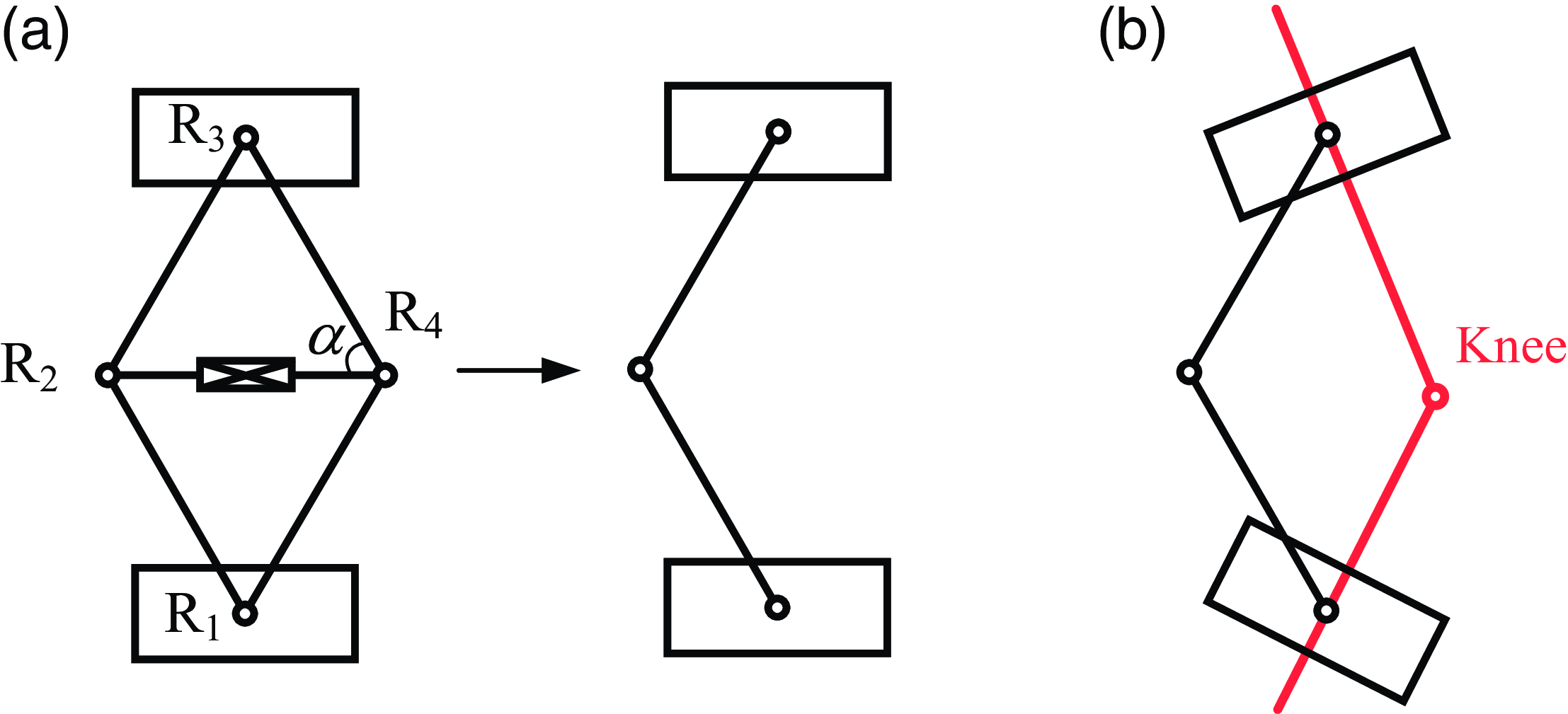
Since the exoskeleton mechanism is strapped to the thigh and calf, its motion is constrained by the human leg. Therefore, it is necessary to consider the human leg and the exoskeleton as a closed-loop mechanism to analyze its DOF. The rhombus linkage mechanism has three DOFs. To simplify the analysis of the DOF of the H-E closed-loop mechanism, the exoskeleton mechanism can be equivalent to a planar serial 3-DOF mechanism, such as a planar serial 3R mechanism (see Figure 4). Project the closed-loop mechanism composed of the serial 3R mechanism and the human lower limb onto the sagittal plane. Obviously, the H-E closed-loop mechanism is a planar four-bar mechanism. Thus, the DOF of the H-E closed-loop mechanism is one.
It is worth noting that although the rhombus linkage mechanism and the serial 3R mechanism have the same DOF and similar kinematic properties, they have different advantages and disadvantages in the application field of knee exoskeletons. The advantage of the serial 3R mechanism is its simple and compact structure, which is easy to design. However, to achieve support for the knee joint, it is necessary to drive the rotation of its rotary joints. In contrast, although the closed-loop rhombus linkage mechanism has a more complex structure, it can support the knee joint without driving the rotary joints. Specifically, the support can be realized by driving the prismatic joint between joints R
 $_2$
and R
 $_4$
. In addition, when the angle
 $\alpha$
between the connecting rods is greater than
 $45^{\circ }$
, the driving force of the linear actuator can amplify the support force. A detailed discussion can be found in Section 4.2. This characteristic of force amplification means that the driving force of the linear actuator does not need to be substantial. Therefore, to a certain extent, it can reduce the performance requirements for the actuator.
Schematic diagram of the H-E closed-loop mechanism. (a) The equivalent mechanism of the rhombus linkage mechanism, that is, the 3R mechanism on the right. (b) Knee exoskeleton closed-loop mechanism.

3. Kinematic modeling
3.1. Exoskeleton mechanism kinematics
The inverse kinematics solution of the exoskeleton mechanism is to solve the length and rotation angle parameters of the driving device based on the known position and orientation parameters of the moving platform (thigh attachment). The geometric schematic diagram of the mechanism is shown in Figure 5. The establishment of the coordinate system is the same as in the previous section. The pose of the platform can be represented by the angle
 $\gamma$
between the
 $Y$
-axis of the coordinate system
 $O-XYZ$
and the
 $y$
-axis of the coordinate system
 $P-xyz$
, along with the coordinates of point
 $P$
, that is,
 \begin{equation} ^{0}\mathbf{P}= \left[\begin{array}{l@{\quad}l@{\quad}l} 0 & P_Y & P_Z \end{array}\right]^T \end{equation}
The lengths of the connecting rods
 $A_1B_1$
,
 $A_1B_2$
,
 $B_1C_1$
, and
 $B_2C_1$
are all
 $l$
. Given the pose of the platform, the input parameters
 $\theta _1$
,
 $l_2$
, and
 $\theta _3$
can be solved through geometric relationships. According to the geometric relationships in Figure 5, we have
 \begin{align} \theta _1=\arccos \frac {P_Y}{\| ^{0}\mathbf{P} \| } -\arccos \frac {\| ^{0}\mathbf{P} \|}{2l} \\[-28pt] \nonumber \end{align}
 \begin{align} l_2=\sqrt {4l^2-\| ^{0}\mathbf{P} \|^{2}} \\[6pt] \nonumber \end{align}
where
 $\theta _1$
is the angle between the
 $A_1B_2$
and the base,
 $l_2$
is the length of the
 $B_1B_2$
, and
 $\theta _3$
is the angle between the
 $B_2C_1$
and the platform.
The coordinates of the point
 $B_2$
in the moving coordinate system are
 \begin{equation} ^{P}\mathbf{B}_2= \left[\begin{array}{l@{\quad}l@{\quad}l} 0 & l\cos \theta _3 & l\sin \theta _3 \end{array}\right]^T \end{equation}
Similarly, the coordinates of the point
 $B_2$
in the base coordinate system are
 \begin{equation} ^{0}\mathbf{B}_2= \left[\begin{array}{l@{\quad}l@{\quad}l} 0 & l\cos \theta _1 & l\sin \theta _1 \end{array}\right]^T \end{equation}
The rotation matrix of the moving coordinate system
 $P-xyz$
with respect to the base coordinate system
 $O-XYZ$
is written as
 \begin{equation} ^{0}_{P}\mathbf{R}= \left[\begin{array}{l@{\quad}l@{\quad}l} 1 & 0 & 0 \\ 0 & \cos \gamma & -\sin \gamma \\ 0 & \sin \gamma & \cos \gamma \end{array}\right] \end{equation}
By expressing the coordinates of point
 $B_2$
in the moving coordinate system
 $P-xyz$
as coordinates in the base coordinate system
 $O-XYZ$
, there is
 \begin{equation} ^{0}\mathbf{B}_2= ^{0}_{P}\mathbf{R} \cdot ^{P}\mathbf{B}_2+^{0}\mathbf{P} \end{equation}
Thus,
 $\theta _3$
can be solved as
 \begin{equation} \theta _3=\arccos \left [ \frac {l\cos (\theta _1-\gamma )-P_Y\cos \gamma -P_Z\sin \gamma }{l} \right ] \end{equation}
The forward kinematics model of the exoskeleton mechanism is determined by three parameters
 $\theta _1$
,
 $l_2$
, and
 $\theta _3$
, which are used in solving the platform pose (
 $\mathbf{P}$
and
 $\gamma$
):
 \begin{align} \| ^{0}\mathbf{P} \| =\sqrt {4l^2-l_{2}^{2}} \\[-24pt] \nonumber \end{align}
 \begin{align} P_Y=\| ^{0}\mathbf{P} \| \cos \left [ \arcsin \Big ( \frac {l_2}{2l} \Big )+\theta _1 \right ] \\[-24pt] \nonumber \end{align}
 \begin{align} P_Z=\| ^{0}\mathbf{P} \| \sin \left [ \arcsin \Big ( \frac {l_2}{2l} \Big )+\theta _1 \right ] \\[-24pt] \nonumber \end{align}
 \begin{align} \gamma =- \left\{\pi - \left [ \arcsin \Big ( \frac {l_2}{2l} \Big )+\theta _1 \right ] +\theta _3 -\arcsin \Big (\frac {l_2}{2l} \Big ) \right\} \\[6pt] \nonumber \end{align}
Geometric diagram of exoskeleton kinematics.

3.2. H-E closed-loop kinematics
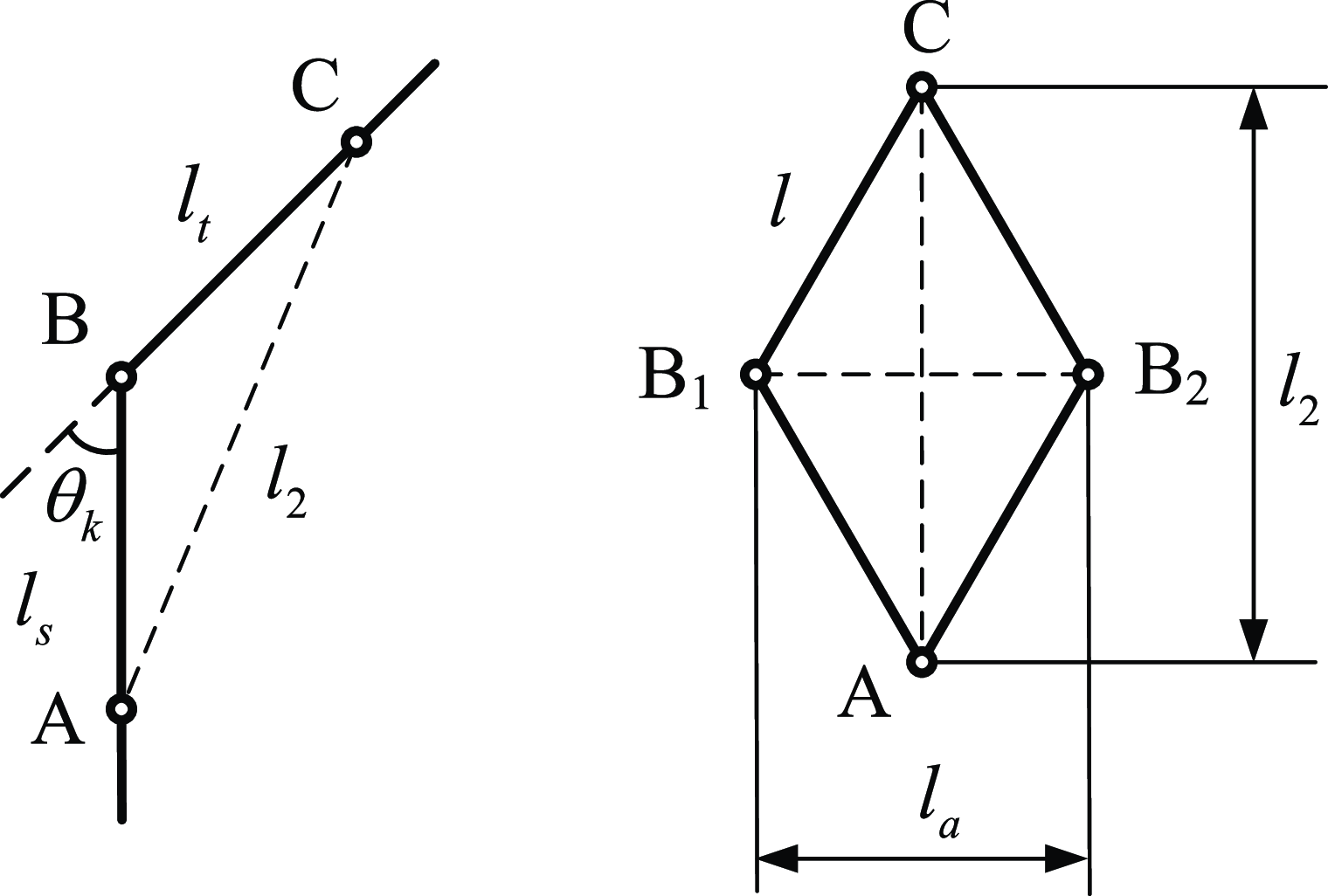
The distance of the active support motion required by the exoskeleton mechanism is related to the motion distance of the driving joints. Moreover, during the stance phase of the gait cycle, the mechanism needs to support the thigh and the calf. During the swing phase of the gait cycle, the mechanism has to swing along with the lower limb, with the driving joints in a free state to adapt to the movement of the knee joint. Thus, the motion pattern of the driving joints is associated with the knee angle in the gait. As depicted in Figure 6, on the left is the simplified model of the thigh, calf, and knee joint, while on the right is the simplified model of the exoskeleton mechanism. Point A represents the revolute joint on the calf attachment, point B is the simplified human biological knee joint, and point C is the revolute joint on the thigh attachment. The lengths of the four connecting rods of the exoskeleton are all
 $l$
. The length
 $l_2$
of the connection point between the thigh and calf attachments can be expressed as
 \begin{equation} l_2=\sqrt {l_{s}^{2}+l_{t}^{2}-2l_sl_t \cos (\pi -\theta _k)} \end{equation}
where
 $l_t$
is the distance from the revolute joint on the thigh attachment to the center of the knee joint,
 $l_s$
is the distance from the revolute joint on the calf attachment to the center of the knee joint, and
 $\theta _k$
is the knee angle.
In the quadrangle
 $AB_1CB_2$
, one has
 \begin{equation} l_{a}^{2}+l_2^{2}=4l^{2} \end{equation}
Combining Eqs. (18) and (19), the connecting rod length of the actuator can be expressed as
 \begin{equation} l_{a}=\sqrt {4l^{2}-l_{s}^{2}-l_{t}^{2}-2l_{s}l_t \cos \theta _k} \end{equation}
where
 $l$
is the length of the linkage of the rhombus linkage mechanism. The right side of Eq. (20) contains only one variable, the knee angle, so the relationship between the length of the actuator and the knee angle is obtained.
Schematic illustration of simplified mechanisms for lower limbs (left) and exoskeleton (right).

3.3. Numerical example
To further illustrate the kinematic characteristics of the mechanism, numerical simulations are carried out using MATLAB software and RecurDyn dynamics software. The simulation model in RecurDyn software is shown in Figure 7(a). Here, the length parameter of the rod is given as
 $l=200$
mm, the angle of the platform
 $\gamma =0^{\circ }$
, and the motion applied to the thigh attachment is defined as
 \begin{equation} P_z=10\sin \left(\frac {2\pi t}{10} \right)+280 \end{equation}
where
 $t$
represents the motion time. As shown in Figure 8, the calculation results of MATLAB software are consistent with the simulation results of RecurDyn, verifying the correctness of the mechanism kinematics. The changes in the three joint angles of the mechanism exhibit a sinusoidal curve, which is consistent with the given motion trend of the platform.
Simulation model. (a) Exoskeleton mechanism. (b) H-E closed-loop mechanism, where the yellow cylinder is the lower limb.

Comparison diagram between theoretical calculation and simulation curves of the joint angles.

According to Eq. (20), the length of the actuator connecting rod is related to the dimensions of the mechanism and the strapping positions on the thigh and calf. Given the strapping distances relative to the knee joint
 $l_s=140$
mm,
 $l_t=140$
mm, as
 $\theta _k$
varies from zero to
 $\pi /2$
, the calculated and simulated curves of the actuator length variation are shown in Figure 9. As the knee flexion angle gradually increases, the length of the actuator connecting rod also gradually increases. This variation relationship is quite intuitive because the flexion of the knee joint will inevitably reduce the distance between point A and point C in Figure 6, thus increasing the distance between points B
 $_1$
and B
 $_2$
.
The relationship between the length of the actuator rod and the knee flexion angle.

Typically, within a walking gait cycle, the knee angle first increases, then decreases, then increases again, and finally decreases [Reference Rose and Gamble46]. Based on this, the curve relationship between the actuator rod length and the knee angle in the gait cycle can be obtained, as shown in Figure 10. The variation law of the actuator rod length is very similar to that of the knee angle in the gait because the relationship between the actuator rod length and the knee angle is close to a linear one (see Figure 9). During the stance phase, the change in the actuator rod length is relatively small, while during the swing phase, the change in the actuator rod length is relatively large, and the driving joint needs to follow the swinging motion of the lower limb.
The relationship between the length of the actuator rod and the knee angle during the gait cycle.

Exoskeleton system wearing schematic diagram.

4. Modeling of exoskeleton actuating system
The exoskeleton system primarily consists of two components: the actuation and control unit (housed in a backpack) and the exoskeleton mechanical structure. As illustrated in Figure 11, the actuation and control unit includes a portable power supply, a controller, joint motors, and a cable-driven unit. The exoskeleton mechanical structure comprises a rhombus linkage mechanism, contour-fitting limb braces, and fastening straps.
The exoskeleton employs a Bowden cable-driven actuation system, which decouples the actuation devices from the execution components. This design avoids the need to directly integrate motors into the linkage structure, thereby maintaining low weight and inertia for the exoskeleton. The Bowden cable consists of an outer Bowden sheath and an inner high-strength rope. The Bowden sheath, a flexible and extensible protective sleeve, guides and protects the rope while accommodating various motion requirements. The rope, characterized by high flexibility and tensile strength, transmits significant forces and torques. A motor in the backpack drives the system by rotating to spool or release the rope. A spool wheel converts the motor’s torque into tensile force on the rope. Spooling the rope generates a contraction motion, which is transmitted to the distal exoskeleton joint and converted into active support forces. Simultaneously, a tension spring is stretched during the spooling process. When the rope is released, the spring restores the exoskeleton mechanism to its initial configuration.
4.1. Mechanical modeling of cable-driven system
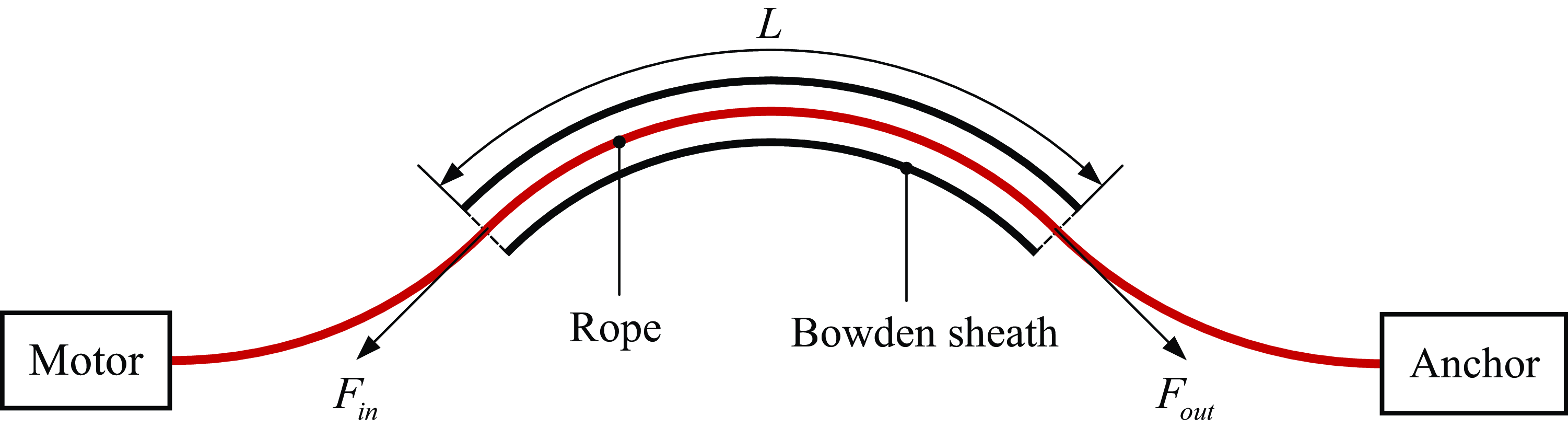
The output force of the cable-driven system will be affected by the friction between the rope and the Bowden sheath, as well as the bending path of the Bowden sheath. Therefore, it is necessary to establish a mechanical model of the cable-driven system to analyze the relationship between the input force and output force of the cable-driven system. The schematic diagram of the Bowden cable-driven unit is shown in Figure 12. The input side includes a motor and a winch, and the output side is connected to the exoskeleton anchor point. The input force and output force are defined as
 $F_{in}$
and
 $F_{out}$
, respectively, and the length of the Bowden sheath is
 $L$
.
Schematic diagram of the Bowden cable-driven unit.

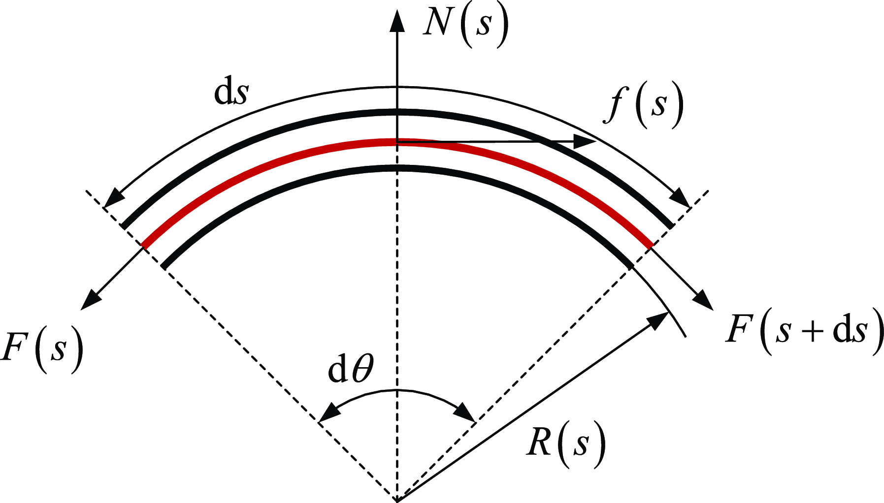
To establish the mechanical model of the Bowden cable, a microelement d
 $s$
of the Bowden cable is taken, and its force analysis is carried out, as shown in Figure 13. It is assumed that the mass of the internal cable of the Bowden cable, as well as the impacts of temperature changes and material fatigue issues on the system, can be neglected. There is only relative motion along the axial direction of the sheath between the outer sleeve and the internal rope of the Bowden cable, and the friction force between the rope and the inner wall of the sheath conforms to the sliding friction formula. The force balance equation of this microelement can be written as
 \begin{align} f(s)+F(s+\mathrm{d}s) \cos \frac {\mathrm{d}\theta }{2} - F(s) \cos \frac {\mathrm{d}\theta }{2} = 0 \\[-24pt] \nonumber \end{align}
 \begin{align} N(s)-F(s+\mathrm{d}s) \sin \frac {\mathrm{d}\theta }{2} - F(s) \sin \frac {\mathrm{d}\theta }{2} = 0 \end{align}
where
 $F(s)$
is the force on the input side of the microelement,
 $f(s)$
is the friction force between the rope and the sheath,
 $N(s)$
is the normal positive pressure of the rope on the sheath,
 $F(s+\mathrm{d}s)$
is the force on the output side of the microelement, and
 $\mathrm{d}\theta$
is the central angle corresponding to the arc length of the microelement.
Mechanical model of the Bowden cable.

Defining the tension difference between the output side and the input side of the microelement as
 $\mathrm{d}F(s)=F(s+\mathrm{d}s)-F(s)$
, the force balance equation of the microelement can be rewritten as
 \begin{align} f(s)=-\mathrm{d}F(s)\cos \frac {\mathrm{d}\theta }{2} \\[-24pt] \nonumber \end{align}
 \begin{align} N(s)=\mathrm{d}F(s) \sin \frac {\mathrm{d}\theta }{2} + 2F(s) \sin \frac {\mathrm{d}\theta }{2} \\[6pt] \nonumber \end{align}
When the microelement is small enough, one has
 $\mathrm{d}F(s) \sin \frac {\mathrm{d}\theta }{2} \approx 0$
,
 $\sin \frac {\mathrm{d}\theta }{2} \approx \frac {\mathrm{d}\theta }{2}$
,
 $\cos \frac {\mathrm{d}\theta }{2} \approx 1$
, thus,
 \begin{align} f(s)=-\mathrm{d}F(s) \\[-24pt] \nonumber \end{align}
 \begin{align} N(s)=F(s)\mathrm{d}\theta \\[6pt] \nonumber \end{align}
According to the friction formula, one has
 \begin{equation} f(s)=\mathrm{sign}(a) \mu N(s) \end{equation}
where
 $a$
represents the motion direction of the rope relative to the Bowden sheath. It is considered positive when its direction is consistent with that of the tension at the input side, and negative otherwise. Also,
 $\mu$
is the friction coefficient.
According to the relationship between the arc length of the element and the center angle, one has
 \begin{equation} \mathrm{d}\theta =\frac {\mathrm{d}s}{R(s)}=\kappa (s)\mathrm{d}s \end{equation}
where
 $R(s)$
is the radius of the element and
 $\kappa (s)$
is the curvature of the element.
Combining Eqs. (26), (27), (28), and (29), one has
 \begin{equation} \frac {\mathrm{d}F(s)}{\mathrm{d}s}=-\mathrm{sign}(a) \mu F(s) \kappa (s) \end{equation}
Define
 $F^{'}(s)$
as the derivative of the tension difference at both ends of the element with respect to the arc length, that is,
 \begin{equation} F^{'}(s)=\frac {\mathrm{d} F(s)}{\mathrm{d} (s)} \end{equation}
Furthermore, we can obtain
 \begin{equation} \frac {F^{'}(s)}{F(s)}=-\mathrm{sign}(a) \mu \kappa (s) \end{equation}
Integrating both sides of it over the interval
 $[s,\ s+\mathrm{d}s]$
, one has
 \begin{equation} \int _{s}^{s+\mathrm{d}s} \frac {F^{'}(s)}{F(s)} \mathrm{d} s = -\mathrm{sign}(a) \mu \int _{s}^{s+\mathrm{d}s} \kappa (s) \mathrm{d} s \end{equation}
If the element curvature
 $\kappa$
can be regarded as a constant, then the tension relationship between the input side and output side of the element can be obtained
 \begin{equation} {F(s+\mathrm{d}s)}=F(s) e^{-\mathrm{sign}(a) \mu \kappa (s) \mathrm{d}s} \end{equation}
Diagram of the relationship between the output force of the Bowden system and the active support force.

Extending to the general case, assuming the same curvature, that is,
 $\theta =\int _{0}^{L} \kappa (s) \mathrm{d}s$
, then the relation between the input force and the output force is
 \begin{equation} F_{out}=F_{in} e^{-\mathrm{sign}(a) \mu \theta } \end{equation}
Considering the movement direction
 $a$
of the rope relative sheath and rewriting (35), the relationship between the input force and the output force of the Bowden cable can be finally obtained as
 \begin{equation} \begin{cases} F_{out}=F_{in} e^{-\mu \theta } & a\gt 0 \\ F_{out}=F_{in} e^{\mu \theta } & a\lt 0 \end{cases} \end{equation}
The internal rope of the Bowden cable is affected by the friction force from the external Bowden sheath. Moreover, the direction of the friction force is related to the direction of the motion tendency, which results in the characteristic of output force hysteresis in the cable-driven system. The relationship between the input force and the output force of the cable-driven system will be described in detail in Section 5.
4.2. Active supporting force of the exoskeleton
The tension of the Bowden cable is transformed into the active supporting force for the human body through the exoskeleton mechanism. The magnitude of this active supporting force is related to the output force of the cable-driven system. As shown in Figure 14, the output force of the Bowden system is converted into a vertical supporting force along the leg. Through the thigh and calf attachment modules of the exoskeleton, the supporting force is transmitted to the thigh and calf, allowing part of the human body’s gravitational load to bypass the knee joint. In other words, the exoskeleton and the knee joint jointly bear the human body’s gravity, thereby reducing the load on the knee joint. Conducting a force analysis on the exoskeleton mechanism, we have
 \begin{equation} \begin{gathered} F_a=2F_c \sin \left(\frac {\pi }{2}-\alpha \right) \\ F_s=2F_c \cos \left(\frac {\pi }{2}-\alpha \right)-F_t \end{gathered} \end{equation}
where
 $F_a$
and
 $F_s$
are the output force of the Bowden cable and the active support force of the exoskeleton, respectively.
 $F_t$
is the elastic force generated by the tension spring between joints R
 $_1$
and R
 $_3$
, which satisfies
 $F_t=k \Delta x_s$
. Here,
 $k$
and
 $\Delta x_s$
are the stiffness coefficient and the deformation of the spring, respectively. By eliminating the component force
 $F_c$
along the connecting rod direction, the relationship between the active supporting force and the output force of the cable-driven system is obtained as
 \begin{equation} F_s=F_a \tan \alpha -k \Delta x_s \end{equation}
The above analysis has dealt with the relationship between the output force and the input force of the cable-driven system, as well as the relationship between the actuator force of the exoskeleton and the active supporting force. Next, the input–output relationship of the entire exoskeleton system from the motor torque to the exoskeleton supporting force will be established. Considering that the output shaft of the motor is connected to a winch to convert the motor torque into the input force of the cable-driven system, we have
 \begin{equation} F_{in}=\frac {M}{R} \end{equation}
where
 $M$
is the motor torque and
 $R$
is the radius of the winch to spool the rope. To simplify the model, it is assumed that the curvature of the Bowden cable path is the same, combining Eqs. (36), (38), and (39), the relationship between the motor torque and the active support force of the exoskeleton can be written as
 \begin{equation} F_{s}=\frac {M}{R} e^{- \mu \theta } \tan \alpha - k \Delta x_s \end{equation}
In addition, considering the rotation angle
 $\alpha _m$
of the motor and referring to Figure 6, under the action of the cable-drive system, the distance between joints R
 $_2$
and R
 $_4$
can be expressed as
 \begin{equation} l_{a}^{\, '}=\frac {1}{2}(l_{a}-\alpha _mR) \end{equation}
Combined with Eq. (41), the relationship between the exoskeleton support displacement
 $X$
and the motor rotation angle can be expressed as
 \begin{equation} X=\sqrt {4l^2-(l_a-\alpha _mR)^2} - l_2 \end{equation}
5. Simulation of the Bowden cable-driven system
In Section 4, the relationship between the input force and output force of the cable-driven system was established. In this section, the output force of the cable-driven system will be simulated to analyze its output characteristics. A 3D model of the Bowden cable is built in CAD software and then imported into RecurDyn software to establish a simulation model. As shown in Figure 15, a fixed constraint is added between the sheath of the Bowden cable and the ground. A surface contact is added between the internal rope and the external sheath of the Bowden cable, and the friction coefficient is set. Taking the friction coefficient of 0.15 and the bending angle of 60
 $^{\circ }$
as an example, the simulation is carried out. An axial force is added between the rope and the ground, and its magnitude is controlled by an expression. A spring is connected between the output end and the ground to measure the output force of the cable-driven system.
Simulation model of the Bowden cable-driven system.

In the simulation, the magnitude of the input force is set to first increase from 0 N to 100 N and then decrease to 0 N. Taking the input force as the abscissa and the output force as the ordinate, the relationship between the input force and output force of the cable-driven system obtained from the simulation is shown in Figure 16(a). When the input force increases, the output force increases approximately linearly. Due to the existence of friction, the maximum actual output force is 84 N, which is lower than the input force. When the input force decreases, also because of friction, the output force remains basically unchanged within a certain range. When the input force drops to about 68 N, the output force then decreases approximately linearly with the input force.
In the simulation, the input force is first increased from 0 N to 100 N, then decreased from 100 N to 50 N, and then increased to 100 N again; the relationship between the input force and output force of the cable-driven system obtained is shown in Figure 16(b). Here, the process of increasing the input force from 0 N to 100 N and then decreasing it from 100 N to 50 N is the same as that in Figure 16(a). When the input force increases from 50 N to 100 N again, the hysteresis of the output force will appear again. The output force remains basically unchanged within a certain range and only starts to increase approximately linearly with the input force after the input force reaches a certain value. By synthesizing the results from Fig. Reference Tan, Shi, Mei, Geng and Yang16(a) and (b), we can derive the relationship between the total input force and the output force of the Bowden cable-drive system. As illustrated in Figure 17, the possible sequences of force application involve two paths: a–b–c and a–b–c–d–a. The curve segment labeled d represents the hysteresis in the output force when the force suddenly transitions from a decreasing phase (corresponding to curve c) to an increasing phase. Similarly, curve segment b depicts the hysteresis that occurs when the force abruptly shifts from an increasing phase (associated with curve a) to a decreasing phase. Furthermore, based on the theoretical model of the cable-driven system in Section 4, the comparison results between the theoretical calculation and the simulation of the relationship between the output force and input force of the cable-driven system are shown in Figure 17. The trends of the two curves are basically the same, which verifies the correctness of the mechanical model of the cable-driven system. In general, due to friction, the output force of the cable-driven system lags behind the input force. That is, segments b and d of the curve in Figure 17 represent the hysteresis, while segments a and c of the curve represent the linear stage of the output force with respect to the input force.
Output force simulation curve of the Bowden cable-driven system. (a) Output force simulation curve where the input force increases from 0 N to 100 N and then decreases to 0 N. (b) Output force simulation curve where the input force increases from 0 N to 100 N, then decreases to 50 N, and finally increases to 100 N. An upward arrow denotes a force increase, and a downward arrow indicates a force decrease.

The comparison curve of theoretical calculation and simulation between the output force and the input force of the Bowden cable-driven system.

In addition to the influence of friction, the output force of the cable-driven system is also affected by the bending angle. Based on the theoretical model of the cable-driven system in Section 4, taking the bending angle and the input force as variables, the output force of the cable-driven system under different input forces and different bending angles can be calculated. The results are shown in Figure 18. When the bending angle is zero, the value of the output force is equal to that of the input force, which means there is no loss of the output force of the cable-driven system when it is not bent. When the input force is non-zero, as the bending angle increases, the output force decreases. That is, the cable-driven system is affected by the bending angle, and part of the output force is lost. Moreover, the larger the bending angle, the smaller the output force.
The relationship between the output force and the input force and the bending angle of the cable-driven system.

Similar to the settings of the simulation model in Figure 15, simulation models of the Bowden cable with bending angles of
 $30^{\circ }$
,
 $60^{\circ }$
,
 $90^{\circ }$
,
 $120^{\circ }$
,
 $150^{\circ }$
, and
 $180^{\circ }$
are established, respectively, as shown in Figure 19. The simulation results at each bending angle are compared with the curve of the relationship between the output force and the bending angle obtained from theoretical calculation and analysis, as shown in Figure 20. The numerical values of the simulation results under these bending conditions are distributed around the theoretical calculation curve and basically coincide with it, which further verifies the correctness of the mechanical model of the cable-driven system. When the value of the input force is fixed, the relationship between the bending angle and the output force is approximately an inverse-proportional linear function; that is, the output force decreases as the bending angle of the Bowden cable increases.
Simulation model of the Bowden cable-driven system under different bending angles.

Comparison of output force simulation and theoretical calculation at different bending angles.

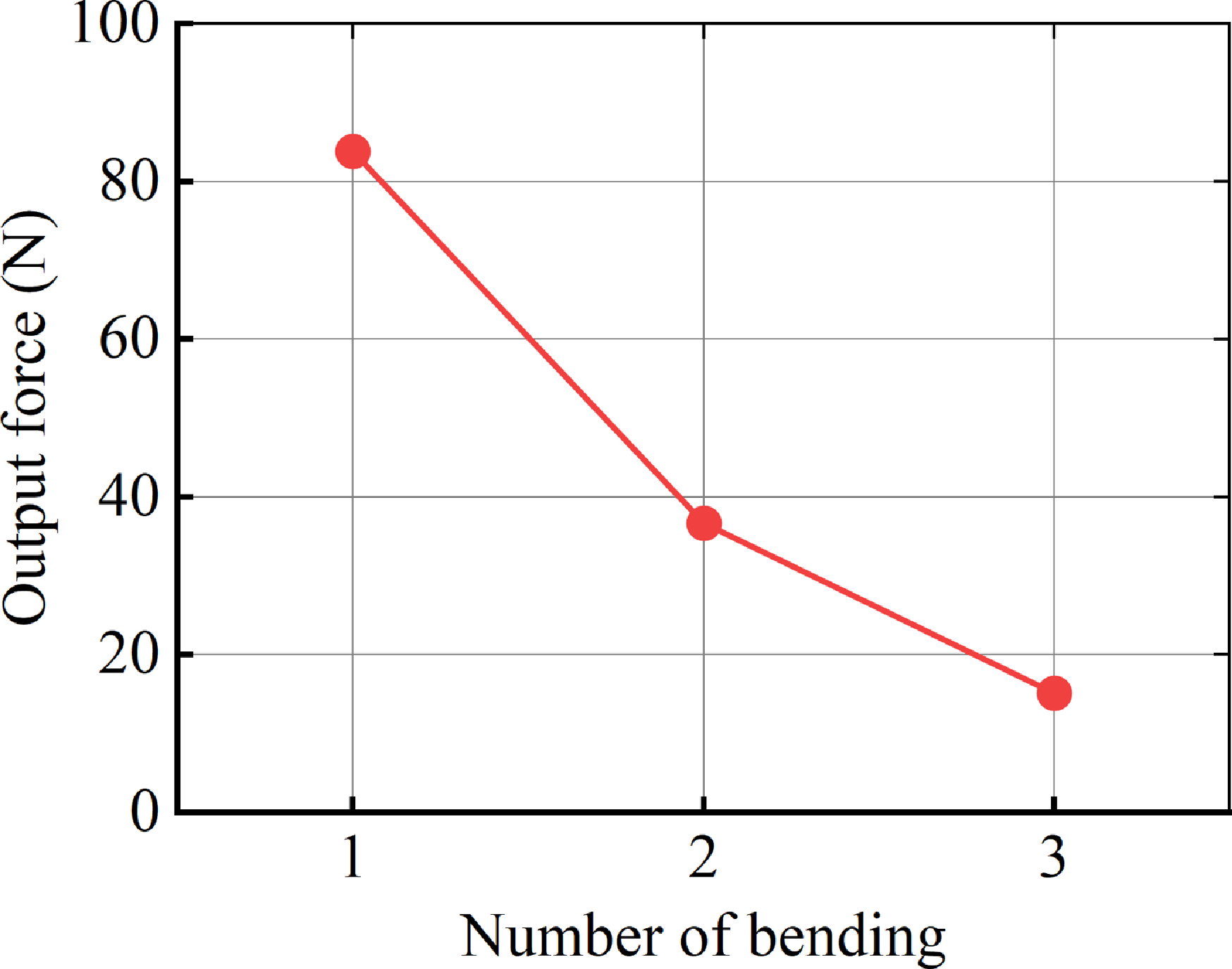
In addition, when the Bowden cable drive system is mounted on the exoskeleton and worn on the human body, in the transmission path from the input end to the output end of the cable-driven system, the number of bends of the Bowden cable will also affect the transmission effect. Next, the influence of the number of bends on the transmission effect of the cable-driven system will be further analyzed through simulation. Simulation models of the cable-driven system with the number of bends ranging from 1 to 3 are established, respectively (see Figure 21). The simulation parameters such as the input force and geometric contact are set the same as those in the previous simulation model, and the internal rope of the cable-driven system is set as a finite-element flexible body. The simulation results of the output force are shown in Figure 22. As the number of bends of the cable-driven system increases, the output force decreases continuously. When the number of bends exceeds 3, the loss of the output force exceeds 80%. Therefore, in the setting of the transmission path of the exoskeleton cable-driven system, the number of bends in the transmission path should be minimized. The fewer the number of bends and the smaller the bending angle, the less the impact on the transmission effect.
Simulation model diagram of the cable-drive system under different bending times.

Simulation results of the relationship between output force and bending times.

6. Exoskeleton wearing experiment
This study consists of three main experiments designed to evaluate the compatibility of the exoskeleton with human motion, its support performance, and its impact on gait, thereby validating the overall performance of the exoskeleton system. First, in the compatibility test, subjects were required to wear the exoskeleton and perform basic daily movements to assess whether the exoskeleton restricts or interferes with natural human motion. Next, for the support performance test, it was considered that a greater support force is not necessarily better—excessive support force may cause discomfort, gait disturbances, or even movement injuries, while insufficient support force may fail to effectively reduce knee joint load. Therefore, this study employs a human-in-the-loop optimization method to repeatedly adjust the output force and motion parameters of the actuation system, ultimately obtaining a set of control parameters that ensure wearing comfort, provide moderate support, and do not interfere with normal gait. Finally, the optimized control strategy was applied to multiple subjects. By comparing and analyzing the changes in lower limb joint kinematic characteristics before and after wearing the exoskeleton, the adaptability of this control strategy to different individual gait patterns was further investigated.
Several typical motion positions while wearing the exoskeletons. (a) Standing on tiptoe. (b) High-knee raising. (c) Deep knee flexion. (d) Forward lunge. (e) Backward lunge. (f) Pushing off the ground with the toes. (g) Mid-stance phase. (h) Step forward. (i) Standing. (j) Sitting position.

6.1. Motion compatibility test
This study first selected a healthy adult male with a height of 180 cm and a body mass of 73 kg for exoskeleton wearability and compatibility testing. As shown in Figure 23, a phased testing approach was adopted: First, the subject wore only the main structure of the exoskeleton (without the cable-driven actuation system) and sequentially performed typical movements, including high knee lifts, deep knee flexion, lunges, normal walking, and sit-to-stand transitions. The experimental results demonstrated that the exoskeleton did not restrict or interfere with the subject’s natural motion in any of the tested movements, and the subject reported no discomfort, confirming the exoskeleton system’s excellent biomechanical compatibility. Notably, the exoskeleton mechanism incorporates an innovative misalignment-free design, effectively avoiding the technical challenge of knee joint rotational axis alignment in traditional exoskeletons, thereby enhancing the adaptability and wearing comfort of the human-exoskeleton system.
6.2. Exoskeleton electromechanical system
The overall structure of the rhombic exoskeleton prototype is shown in Figure 24, where the rod length of the rhombus mechanism is 160 mm. The exoskeleton mechanism connects to the thigh and shank through customized braces at both ends. To achieve optimal fit between the braces and lower limbs, we first acquired 3D geometric data of the lower limbs using laser scanning. Based on this scan data, we designed anatomically conforming braces that precisely match the limb contours, which were then fabricated using additive manufacturing technology. The inner surface of each brace incorporates a flexible liner with silicone particle padding. This design serves dual purposes: enhancing wearer comfort while preventing slippage during motion through improved frictional properties.
Exoskeleton electromechanical system and its overall wearing illustration. (a) Rhombic mechanism part of the exoskeleton. (b) Overall wearing illustration of the exoskeleton. (c) Actuating and control unit. (d) Input end of the Bowden cable-drive system (including the motor, winch, and PE wire). (e) Force-sensitive resistor unit for detecting gait events.

The actuation and control unit employs a modular integrated design, with all components mounted on a backpack. The system core consists of an STM32 F407 embedded controller. Beneath the control board lies a lithium battery that powers both the controller and motors. The actuation system utilizes a Bowden cable mechanism. At the input end, a motor (Xiaomi CyberGear, China) coupled with a 20 mm radius winch forms the driving component (see Figure 24(d)). Each Bowden cable comprises an outer sheath and an inner core made of ultra-high molecular weight polyethylene (PE) fishing line (Aosite, 1.2 mm diameter, China). The output ends of the Bowden cables connect to joints R
 $_2$
and R
 $_4$
of the rhombic mechanism. During operation, motor rotation tightens the PE lines via the winch, converting the motor torque into tensile force on the PE lines. This force reduces the distance between joints R
 $_2$
and R
 $_4$
, thereby generating a vertical support force to alleviate knee joint loading. Concurrently, extension springs (with a stiffness coefficient of 0.09 N/mm) between joints R
 $_1$
and R
 $_3$
store energy. Upon motor release, the springs’ elastic restoring force returns the system to its initial state, completing a full support cycle.
To enable the exoskeleton to provide supporting force at the appropriate timing, a force-sensitive resistor (FSR) unit (Ruiboyi, 30
 $\times$
60 mm, China) was installed at the heel area as the triggering sensor for the actuation system. As shown in Figs. 24(e) and 25(c), this sensor precisely detects the initial contact moment of the stance phase in the gait cycle by monitoring pressure-induced resistance changes (manifested as resistance drop) during heel strike. To ensure measurement accuracy, a specialized protective structure was implemented: both surfaces of the thin-film FSR were reinforced with rigid circular plates, and the entire assembly was encapsulated using waterproof adhesive tape. This design effectively eliminates measurement errors caused by sensor bending deformation while simultaneously ensuring durability and reliability.
6.3. Human-in-the-loop optimization
The FSR-triggered control strategy for the exoskeleton system is illustrated in Figure 25(a). When heel strike occurs and the FSR detects plantar pressure exceeding the predefined threshold, the control motor activates, causing the Bowden cable system to contract and generate tension in the PE lines. When the pressure falls below this threshold, the motor releases and the Bowden cable system resets.
Human-in-the-loop optimization experiment. (a) Control strategy of exoskeleton system triggered by FSR. (b) Exoskeleton system and Bowden cable output force measurement sensor (1-D force sensor). (c) FSR pasted on the heel

Since direct measurement of the exoskeleton’s supportive force on human limbs is challenging without installing sensors on the thigh or shank, an indirect approach was adopted by monitoring the tension in the PE lines (Bowden cable output force) to evaluate the support force (the conversion relationship between Bowden cable driving force and support force is detailed in Section 4.2). At the Bowden cable output end, between joints R
 $_2$
and R
 $_4$
, 1-D force sensors (ZNLBS-VI-50 KG, Znsensor, China, 50 Hz) were installed on both medial and lateral sides of the knee to collect line tension data. As shown in Figure 25(b) and (c), the system employs an FSR-triggered control strategy. The FSR sensor attached to the heel monitors the initial contact phase of gait in real-time, while the motor operates in position control mode. Through human-in-the-loop optimization, control parameters were iteratively adjusted. During optimization, subjects walked on a treadmill at 3 km/h for approximately 1-min per test. After multiple iterations, the optimal control parameters were determined (motor rotation: 13 rad, speed: 25 rad/s). This configuration provides substantial support while maintaining natural gait patterns. Figure 26 displays the averaged and normalized Bowden cable output force curve, derived from a complete gait cycle analysis during one minute of walking tests.
During the initial stance phase of gait, the Bowden cable output force demonstrates an approximately sinusoidal increasing trend, reaching its peak during mid-stance. Experimental data show that the peak tension values recorded by the medial and lateral knee sensors were 38.2
 $\pm$
5.6 N (mean
 $\pm$
SD) and 39.2
 $\pm$
5.2 N (mean
 $\pm$
SD), respectively. As the gait transitions into the swing phase (accounting for 60–100% of the gait cycle), the system actively releases the motor, allowing cable tension to rapidly decay to zero. This dynamic force control strategy ensures unrestricted knee flexion–extension during the swing phase, thereby inherently avoiding gait perturbation.
Human-in-the-loop optimized Bowden cable output force profile.

6.4. Gait experiment
To validate the adaptability of the optimized Bowden cable output force profile across different individuals, this study conducted a multi-subject gait adaptation experiment involving five healthy male participants (coded S1-S5) with a mean height of 178
 $\pm$
2.5 cm (mean
 $\pm$
SD) and body mass of 69.8
 $\pm$
3.2 kg (mean
 $\pm$
SD). The experiment adopted a controlled design where baseline natural gait data were first collected during 1-min walking trials at 3 km/h without exoskeleton assistance, followed by trials under identical conditions with exoskeleton engagement (experimental setup shown in Figure 27). A high-precision optical motion capture system (Mars, Nokov, China) recorded lower-limb kinematic data in both conditions. To ensure data reliability, dozens of gait cycles collected within 1 min were temporally normalized to percentage-based gait phases and ensemble averaged, ultimately generating the sagittal-plane joint angle profiles presented in Figure 28.
Experimental scene of the experimenter walking while wearing the exoskeleton.

Joint kinematic data of participants (S1–S5), where solid lines represent the averaged joint angle curves from 1-min walking trials, and shaded areas indicate
 $\pm$
1 standard deviation.

7. Discussion
It was observed that when the linkage angle
 $\alpha \gt 45^{\circ }$
, the exoskeleton’s rhombic mechanism exhibits a force amplification effect on the Bowden cable output. Consequently, the supportive force applied to the thigh must exceed the sum of the medial and lateral cable tensions. Under maximum support conditions (corresponding to 30 mm spring displacement, 2.7 N elastic force, and
 $\alpha = 68.7^{\circ }$
), the system amplifies the peak Bowden cable output (totaling approximately 77.4 N from both cables) to 195.8 N of vertical support force, equivalent to 28.6%
 $\pm$
3.7% (mean
 $\pm$
SD) of the subject’s body weight. This mechanical amplification constitutes the key feature enabling the exoskeleton’s efficient support performance.
Comparative analysis with existing studies shows that (1) the body weight support system proposed in Ref. [Reference Ikeuchi, Ashihara, Hiki, Kudoh and Noda39] provides a maximum vertical support force of 100 N; (2) the passive exoskeleton system in Ref. [Reference Lovrenovic and Doumit47] delivers support forces ranging from 253 to 571 N, corresponding to 9.41–26.18% of the subject’s body weight; and (3) the weight-support lower extremity exoskeleton presented in Ref. [Reference Wang, Lee and Ji41] reduces plantar pressure by 21.9% during the stance phase. However, these exoskeletons feature relatively complex structures, and experiments also demonstrated that excessive support forces can interfere with normal walking. In contrast, the active support exoskeleton developed in this study achieves comparable biomechanical support effectiveness while maintaining a simpler structural design.
As shown in Figure 28, the lower limb joint kinematic curves of all five subjects demonstrated similar overall trends before and after exoskeleton wearing, though observable subtle differences were present. During the stance phase, subjects S1, S4, and S5 exhibited slightly reduced hip flexion angles when wearing the exoskeleton compared to the non-wearing condition, with a maximum decrease of 7
 $^{\circ }$
(occurring at approximately 20% of the gait cycle for S1). In contrast, the hip movement patterns of S2 and S3 remained largely unaffected. For knee joint kinematics during the stance phase, subjects S1, S2, and S3 showed increased flexion angles when wearing the exoskeleton, with a maximum deviation of 7
 $^{\circ }$
observed at around 10% of S2’s gait cycle. During swing phase, peak knee flexion angles decreased for subjects S1–S4, with S2 showing the largest reduction (8
 $^{\circ }$
), followed by S4 (3.3
 $^{\circ }$
), S1 (2.2
 $^{\circ }$
), and S3 (0.8
 $^{\circ }$
). Ankle joint kinematics during the stance phase remained consistent across all subjects, except for S3, who displayed a unique ankle movement pattern in the non-wearing condition—maintaining nearly constant ankle angles between 10 and 20% of the gait cycle, potentially related to individualized gait strategies. Notably, despite these observed subtle kinematic alterations, none of the subjects reported wearing discomfort. These results indicate that the physical human-exoskeleton interaction established by our system remains within physiologically acceptable limits, without causing significant movement compensation or adverse reactions.
Through comprehensive evaluations including human-exoskeleton compatibility tests, Bowden cable force optimization, and multi-subject gait experiments, this study has systematically assessed the exoskeleton’s human adaptability and support performance. However, it should be noted that the current research still presents certain limitations. The implemented control strategy remains relatively basic, requiring time-consuming and labor-intensive human-in-the-loop optimization processes to iteratively adjust motor parameters for achieving Bowden cable output force profiles that simultaneously ensure support effectiveness and maintain natural gait patterns. Future research should focus on developing adaptive control algorithms capable of intelligently recognizing human gait characteristics and providing assistance at optimal timings. Such improvements are expected to further enhance the exoskeleton’s support efficacy beyond current levels while minimizing interference with natural gait kinematics.
8. Conclusion
This study presents a novel rhombic-mechanism knee exoskeleton with a simple structure and alignment-free design that achieves dual functionality of adaptive knee motion and active weight support. The research establishes kinematic models for both the rhombic mechanism and the human-exoskeleton closed-loop system, with numerical simulations validating the model accuracy. For the cable-driven actuation system, mechanical modeling clarifies the force transmission relationship between cable input/output and the conversion mechanism from motor torque to support force, while simulations analyze the Bowden cable’s output characteristics under various bending conditions. The mechatronic system of the exoskeleton was demonstrated, and motion compatibility experiments showed that the exoskeleton does not interfere with human movement under several typical motion postures. Human-in-the-loop optimization was used to obtain the optimized output force curve of the Bowden cable, while joint kinematics from multiple test subjects indicated that wearing the exoskeleton caused acceptable variations in joint kinematics. Ultimately, the exoskeleton system was validated to exhibit excellent motion adaptability and effective active support performance.
Author contributions
Yu Guo and Xiangyu Yan wrote the article. Xiao Yang developed the exoskeleton prototype. Ziming Chen and Fei Liu conceived and designed the study.
Financial support
This work was supported in part by the National Natural Science Foundation of China (Grant 52275035) and in part by the Natural Science Foundation of Hebei Province of China (Grant E2023203109).
Competing interests
The authors declare no conflicts of interest exist.
Ethical approval
This work involved human subjects and has been approved by the local ethics committee (First Hospital of Qinhuangdao).