INTRODUCTION
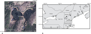
The northeastern United States (NE USA) experienced multivariate patterns of climate change, including seasonal differences in temperature during the late Pleistocene–early Holocene transition from a glacial to an interglacial climate. Global shifts in insolation and atmospheric CO2 combined with regional feedbacks related to ice sheet dynamics and abrupt changes in ocean heat transport and sea ice extent heavily modified climate trends in the North Atlantic region (Denton et al., Reference Denton, Anderson, Toggweiler, Edwards, Schaefer and Putnam2010; Clark et al., Reference Clark, Shakun, Baker, Bartlein, Brewer, Brook, Carlson, Cheng, Kaufman and Liu2012). Cooling centered over the North Atlantic during the Younger Dryas chronozone (YD, 12.9–11.7 cal ka BP) caused a reversal of the long-term warming trend (Ruddiman and McIntyre, Reference Ruddiman and McIntyre1981; Rind et al., Reference Rind, Peteet, Broecker, McIntyre and Ruddiman1986; Dansgaard et al., Reference Dansgaard, White and Johnsen1989). Although many paleoclimate records from the NE USA and adjacent Canada also indicate cooling during the YD (e.g., Cwynar and Levesque, Reference Cwynar and Levesque1995; Mayle and Cwynar, Reference Mayle and Cwynar1995b; Hou et al., Reference Hou, Huang, Oswald, Foster and Shuman2007), there is not always alignment across proxies, and there is evidence of regional variability (Yu and Eicher, Reference Yu and Eicher1998; Cwynar and Spear, Reference Cwynar and Spear2001; Shuman et al., Reference Shuman, Webb, Bartlein and Williams2002b; Gonzales and Grimm, Reference Gonzales and Grimm2009). Additionally, while multiple records from the North Atlantic and northwestern Europe suggest an unstable and more variable climate during the latter part of the YD (McManus et al., Reference McManus, Francois, Gherardi, Keigwin and Brown-Leger2004; Bakke et al., Reference Bakke, Lie, Heegaard, Dokken, Haug, Birks, Dulski and Nilsen2009; Carlson et al., Reference Carlson, Clark, Haley, Klinkhammer, Simmons, Brook and Meissner2007; Elmore and Wright, Reference Elmore and Wright2011; Pearce et al., Reference Pearce, Seidenkrantz, Kuijpers, Massé, Reynisson and Kristiansen2013), evidence for YD temporal variability in northeastern North America is limited (Yu and Eicher, Reference Yu and Eicher1998; Gonzales and Grimm, Reference Gonzales and Grimm2009; Watson et al., Reference Watson, Williams, Russell, Jackson, Shane and Lowell2018). There is also evidence from the NE USA for the continuation of centennial-scale climatic variability into the early Holocene, although the climatic significance, regional extent, and causes of these changes are not clear (e.g., Anderson et al., Reference Anderson, Mullins and Ito1997, Reference Anderson, Levac and Lewis2007; Yu and Eicher, Reference Yu and Eicher1998; Kirby et al., Reference Kirby, Patterson, Mullins and Burnett2002a; Ellis et al., Reference Ellis, Mullins and Patterson2004; Mullins et al., Reference Mullins, Patterson, Teece and Burnett2011; Hou et al., Reference Hou, Huang, Shuman, Oswald and Foster2012). Finally, the teleconnections between changes in the North Atlantic and upwind regions are not fully understood and were likely overshadowed by the influence of continental climatic factors, including the lingering presence of the Laurentide Ice Sheet and the larger impacts of increasing summer insolation on the continent (Rind et al., Reference Rind, Peteet, Broecker, McIntyre and Ruddiman1986; Fawcett et al., Reference Fawcett, Ágústsdóttir, Alley and Shuman1997; Manabe and Stouffer, Reference Manabe and Stouffer1997). This paper takes a multiproxy approach to reconstruct the sequence of environmental change from 13.5 to 9.0 cal ka BP at Twin Ponds, VT, and addresses some of the uncertainties surrounding the Pleistocene–Holocene transition in the NE USA (Fig. 1). We focus first on the YD and then on early Holocene variability.
(A) Site and bathymetric map of Twin Ponds showing the location of core 48 along the littoral zone on west Twin Ponds. (B) Regional map showing location of Twin Ponds relative to other sites with previous evidence for climate change during and after the Younger Dryas. 1, Crawford Lake; 2, Twiss Marl Pond (Yu and Eicher, Reference Yu and Eicher1998); 3, Fayetteville Green Lake (Kirby et al., Reference Kirby, Patterson, Mullins and Burnett2002a, Reference Kirby, Mullins, Patterson and Burnett2002b); 4, Pond of Safety; 5, Lake of the Clouds; 6, Lost Lake (Cwynar and Spear, Reference Cwynar and Spear2001); 7, Winneconnet Pond (Suter, Reference Suter1987); 8, Rogers Lake (Davis, Reference Davis1969); 9, Moulton Pond (Davis et al., Reference Davis, Bradstreet, Stuckenrath and Borns1975); 10, Trout Pond; 11, Tilley Pond (Cwynar and Levesque, Reference Cwynar and Levesque1995); 12, Splan Pond (Mayle and Cwynar, Reference Mayle and Cwynar1995b; Walker et al., Reference Walker, Mott and Smol1991); 13, Killarney Lake (Levesque et al., Reference Levesque, Mayle, Walker and Cwynar1993).

Most paleoenvironmental records from the NE USA and eastern Canada show some evidence of climate change during the YD (e.g., Mott et al., Reference Mott, Grant, Stea and Occhietti1986; Peteet et al., Reference Peteet, Vogel, Nelson, Southon, Nickmann and Heusser1990; Levesque et al., Reference Levesque, Mayle, Walker and Cwynar1993; Anderson and Macpherson, Reference Anderson and Macpherson1994; Yu and Wright, Reference Yu and Wright2001; Shuman et al., Reference Shuman, Webb, Bartlein and Williams2002b; Fig. 1). Loss-on-ignition (LOI) records show a consistent decrease in organic carbon during the YD that has been attributed to a decline in aquatic productivity (Shuman et al., Reference Shuman, Newby, Huang and Webb2004; Thompson et al., Reference Thompson, Dorion, Ridge, Balco, Fowler and Svendsen2017) and increased erosion (Levesque et al., Reference Levesque, Mayle, Walker and Cwynar1993; Yu and Eicher, Reference Yu and Eicher1998; Cwynar and Spear, Reference Cwynar and Spear2001). Lacustrine oxygen isotope records from the northeast also show a regionally coherent decline during the YD that suggests cold conditions (Anderson et al., Reference Anderson, Mullins and Ito1997; Kirby et al., Reference Kirby, Mullins, Patterson and Burnett2002b; Zhao et al., Reference Zhao, Yu, Ito and Zhao2010; Mandl et al., Reference Mandl, Shuman, Marsicek and Grigg2016). Pollen records from the region are more spatially variable and do not always indicate unequivocal cooling; records from maritime Canada, Maine, southern New England, and the southern Great Lakes suggest a definitive cooling during the YD (Davis, Reference Davis1969; Suter, Reference Suter1987; Mayle and Cwynar, Reference Mayle and Cwynar1995a; Gonzales and Grimm, Reference Gonzales and Grimm2009; Watson et al., Reference Watson, Williams, Russell, Jackson, Shane and Lowell2018), whereas those from New Hampshire and southern Ontario do not (Spear, Reference Spear1989; Spear et al., Reference Spear, Davis and Shane1994; Yu and Eicher, Reference Yu and Eicher1998). High-resolution pollen and branched glycerol dialkyl glycerol tetraether records from the southern Great Lakes indicate increased moisture during the YD and cooling that began 300–400 years after its onset in the North Atlantic (Gonzales and Grimm, Reference Gonzales and Grimm2009; Watson et al., Reference Watson, Williams, Russell, Jackson, Shane and Lowell2018). Chiromonid water temperature reconstructions from maritime Canada and Maine confirm cooling during both the YD summer and winter (Walker et al., Reference Walker, Mott and Smol1991; Cwynar and Levesque, Reference Cwynar and Levesque1995; Mayle and Cwynar, Reference Mayle and Cwynar1995b); however, in the White Mountains of New Hampshire, the chiromonid record reflects less summer cooling than at the coastal sites (Cwynar and Spear, Reference Cwynar and Spear2001).
East–west gradients observed in both the pollen and chiromonid data point to coastal versus inland climatic factors as an explanation for some of the observed YD spatial diversity (Cwynar and Spear, Reference Cwynar and Spear2001; Shuman et al., Reference Shuman, Webb, Bartlein and Williams2002b). Paleoclimate models show the greatest YD cooling during the winter along the northeastern coast of North America and warmer summer temperatures at inland locations (Rind et al., Reference Rind, Peteet, Broecker, McIntyre and Ruddiman1986; Manabe and Stouffer, Reference Manabe and Stouffer1997). Others have proposed that the lack of a pollen signal during the YD at some sites may be dependent on the location of the site relative to an ecotone, with sites closer to an ecotone being more sensitive to climate change than those far from the ecotone (Cwynar and Levesque, Reference Cwynar and Levesque1995; Yu and Eicher, Reference Yu and Eicher1998); other analyses indicate the reverse and raise questions about the potential sensitivity of ecotones to rapid climate changes (Shuman et al., Reference Shuman, Webb, Bartlein and Williams2002b).
Evidence for post-YD variability in the NE USA and adjacent Canada falls into two different categories. One category of evidence shows a series of brief (150–250 year) cold periods that have been linked with continued freshwater influxes into the North Atlantic from melting ice sheets and subsequent changes in sea-surface temperatures (SSTs) and Atlantic meridional overturning circulation (Broecker, Reference Broecker1990; Clark et al., Reference Clark, Marshall, Clarke, Hostetler, Licciardi and Teller2001; Fisher et al., Reference Fisher, Smith and Andrews2002; Teller et al., Reference Teller, Leverington and Mann2002). These include a cold interval at 11.3 cal ka BP, known from North Atlantic and European records as the Preboreal Oscillation (Björck et al., Reference Björck, Kromer, Johnsen, Bennike, Hammarlund, Lemdahl, Possnert, Rasmussen, Wohlfarth and Hammer1996, Reference Björck, Rundgren, Ingolfsson and Funder1997; Rasmussen et al., Reference Rasmussen, Vinther, Clausen and Andersen2007). A similar cold event has been identified in oxygen isotope records from Ontario, New York, and New Jersey (Anderson et al., Reference Anderson, Mullins and Ito1997; Yu and Eicher, Reference Yu and Eicher1998; Ellis et al., Reference Ellis, Mullins and Patterson2004; Zelanko et al., Reference Zelanko, Yu, Bebout and Kaufman2012) and in pollen records from the Gulf of St. Lawrence region, Canada (Anderson et al., Reference Anderson, Levac and Lewis2007). Compound-specific hydrogen isotope and carbonate oxygen isotope records from Massachusetts, New Jersey, and Ontario suggest a series of additional early Holocene cold intervals at ca. 10.6, 10.2, 9.5, 9.3, 8.8, and 8.2 cal ka BP (Yu and Eicher, Reference Yu and Eicher1998; Hou et al., Reference Hou, Huang, Oswald, Foster and Shuman2007, Reference Hou, Huang, Shuman, Oswald and Foster2012; Yu, Reference Yu2007). Although pollen records from the NE USA generally do not show evidence for these cool periods, there is widespread evidence for vegetation change at ca. 8.2 cal ka BP that aligns with a prominent cold period seen in North Atlantic and European records (Alley et al., Reference Alley, Mayewski, Sowers, Stuiver, Taylor and Clark1997; Shuman et al., Reference Shuman, Bartlein, Logar, Newby and Webb2002a, Reference Shuman, Newby and Donnelly2009; Veski et al., Reference Veski, Seppä and Ojala2004). The second type of post-YD variability that has been described in the NE USA is a broad plateau in oxygen isotope records from New York, Vermont, and New Jersey from ca. 11.5 to 10.0 cal ka BP (Kirby et al., Reference Kirby, Patterson, Mullins and Burnett2002a; Zhao et al., Reference Zhao, Yu, Ito and Zhao2010; Mandl et al., Reference Mandl, Shuman, Marsicek and Grigg2016). Kirby et al. (Reference Kirby, Patterson, Mullins and Burnett2002a) attribute this positive interval of δ18O values to an expanded trough in the polar vortex that allowed southern-sourced precipitation to flow into the northeast.
This paper presents pollen and ostracode records from Twin Ponds, VT (Fig. 1) that build upon previously published oxygen isotope and LOI records from the same core (Mandl et al., Reference Mandl, Shuman, Marsicek and Grigg2016). The record extends from 13.5 to 9.0 cal ka BP and further explores both spatial and temporal climatic variability during and after the YD. Twin Ponds is positioned along an east–west gradient between published sites in maritime Canada and Maine and those in the Great Lakes region and provides a further test for the presence of coastal versus inland climatic variability (Fig. 1). The northerly location of Twin Ponds also provides a contrast to sites in southern New England that were located within different types of boreal ecosystems after deglaciation (Jacobson et al., Reference Jacobson, Webb, Grimm, Ruddiman and Wright1987; COHMAP, 1988). The multiproxy approach of this study allows the different types of aquatic versus terrestrial biotic responses to be compared with one another and with abiotic (sedimentary, geochemical) changes to provide a more accurate environmental reconstruction. A change in only one or two proxies may be explained by any number of environmental factors that were independent of climate, whereas the alignment of all proxies provides a strong case for a climatic cause. General environmental and climatic reconstructions are made for both the late Pleistocene (>11.7 cal ka BP) and the early Holocene (<11.7 cal ka BP) and for centennial-scale changes consistent across multiple proxies.
Study Site
Twin Ponds is located in Brookfield, VT (44°01′41.6″N, 72°34′45.6″W, 372 m elevation) within two connected basins with a maximum depth of 7 m in the west basin and 9 m in the east basin (Fig. 1). Twin Ponds is fed by one small permanent inlet located in the northwest part of the western basin and multiple seasonal groundwater seeps that enter through a fringing sedge wetland. The outlet for Twin Ponds is located at the southern end of the east basin and is a tributary of the Second Branch of the White River. Twin Ponds is one of many ponds that occupy basins along strike within the Devonian-aged Waits River Formation, composed of carbonaceous phyllite and limestone (Ratcliffe et al., Reference Ratcliffe, Stanley, Gale, Thompson, Walsh, Rankin, Doolan, Kim, Mehrtens and Aleinikoff2011). The ponds were formed during deglaciation of the Laurentide Ice Sheet between 14.5 and 14.0 cal ka BP (Ridge et al., Reference Ridge, Balco, Bayless, Beck, Carter, Dean, Voytek and Wei2012) that left behind numerous scoured basins, particularly within more soluble CaCO3-rich bedrock. The ponds are immediately surrounded by rich northern hardwood forest dominated by Acer saccharum (sugar maple), Fagus grandiflora (American beech), and Tsuga canadensis (eastern hemlock) (Thompson and Sorenson, Reference Thompson and Sorenson2000). The climate of this region is cool-temperate and moist with an average annual precipitation of 112 cm, a mean temperature of the coldest month (January) of −9.35°C, and a mean temperature of the warmest month (July) of 18.55°C (National Weather Service, w2.weather.gov/climate. Accessed June 2020).
There are several distinct depositional environments within Twin Ponds that provide important context for paleoenvironmental reconstructions. The influence of groundwater rich in dissolved Ca2+ and HCO3− results in high alkalinity (ca. 140 mg/L as CaCO3) and supports a dense mat of the macro algae Chara sp. on the littoral benches up to a depth of ca. 3.5 m. Intense photosynthetic activity in the microzone surrounding Chara cells leads to a reduction in CO2 and the inorganic precipitation of CaCO3 encrustations on the stem- and leaf-like cells (Wetzel, Reference Wetzel1960). The fragments of these encrustations accumulate in the littoral zone, forming sedimentary benches. The composition of the littoral sediment currently ranges between 70% and 90% inorganic carbon and 5% and 10% organic carbon. In contrast, phytoplankton are the dominant primary producers in the deeper, seasonally anoxic areas of the ponds (ca. 3.5–9.0 m depth) where the sediment is composed of 30%–60% organic carbon and 5%–10% inorganic carbon. On the landward side of the littoral zone, a fringing sedge wetland leads to the development of a fibrous peat and the highest percentages of organic carbon (50%–80%) and low (<5%) inorganic carbon.
METHODS
Core collection, LOI, δ18O, and X-ray fluorescence (XRF)
The cores were collected from the Chara-rich littoral bench on the east side of the west basin at a water depth of ca. 0.5 m (Fig. 1). A Livingstone piston corer with a 70-mm-diameter Bolivia attachment was used to collect three 1-m-long cores during the fall of 2012. Sampling, core imaging, and LOI analyses were done at the University of Wyoming and are fully described by Mandl et al. (Reference Mandl, Shuman, Marsicek and Grigg2016). LOI burns at 550° and 1000°C were used to determine percentages of organic and inorganic carbon, respectively (Dean, Reference Dean1974). Eight samples from the late-glacial interval were previously analyzed by XRF analysis at the U.S. Geological Survey in Denver, CO (Serravezza, M. personal communication) and provided a limited mineralogical survey on the changing weight percent of clay minerals. The weight percentages of the clay minerals were used as an indication of the relative abundance of allocthonous minerogenic material.
The preparation and measurement of <63 μm bulk carbonate for stable isotope analysis is described fully by Mandl et al. (Reference Mandl, Shuman, Marsicek and Grigg2016). This fraction of CaCO3 is primarily composed of inorganically precipitated CaCO3 and reflects the isotopic composition of water at the depth and time of formation. Inorganic precipitation of CaCO3 in the littoral zone of Twin Ponds currently occurs during the growing season at depths between ca. 20 cm and 2 m. Oxygen isotope values of the bulk carbonate were measured at the University of Wyoming Stable Isotope Facility using a Thermo Finnigan Delta Plus XP mass spectrometer, a CTC Analytics gas chromatography PAL autosampler and a Thermo Finnigan GasBench II and were reported with 2ơ standard uncertainty (0.2‰).
The oxygen isotope values of the ostracode shells were measured at the University of Minnesota on a Finnigan MAT252 mass spectrometer with a Kiel device. Shells of common species of benthic and nektic ostracodes were carefully selected and cleaned following the methods of Xia et al. (Reference Xia, Haskell, Engstrom and Ito1997). Multiple shells of the same species within a sample were selected, with the number based on the size of the species: 4–5 adult valves for benthic species and 15–30 adult valves for nektic species. Reaction with phosphoric acid followed, and the isotopic ratio of the released CO2 gas was analyzed following standard methods (Ito and Forester, Reference Ito and Forester2017). Quality assurance/quality control procedure included analysis of NBS-19 for every eight samples. All isotopic values are reported as the per mil (‰) deviation from the VPDB standard. In midlatitudes of the Northern Hemisphere, benthic species can live more than a year at the sediment–water interface and molt throughout the seasons as they grow, whereas nektic species tend to live among the aquatic plants in the littoral zone during the spring and summer and typically have a shorter life span. One consequence of this difference is that nektic species tend to reflect surface-water isotopic values for the spring and summer months, while benthic species are a better indicator of annual bottom-water isotopic values (Dettman et al., Reference Dettman, Smith, Rea, Moore and Lohmann1995; Oleskiewicz, Reference Oleskiewicz1998; Bacon, Reference Bacon1999; Jones, Reference Jones2002).
Chronology
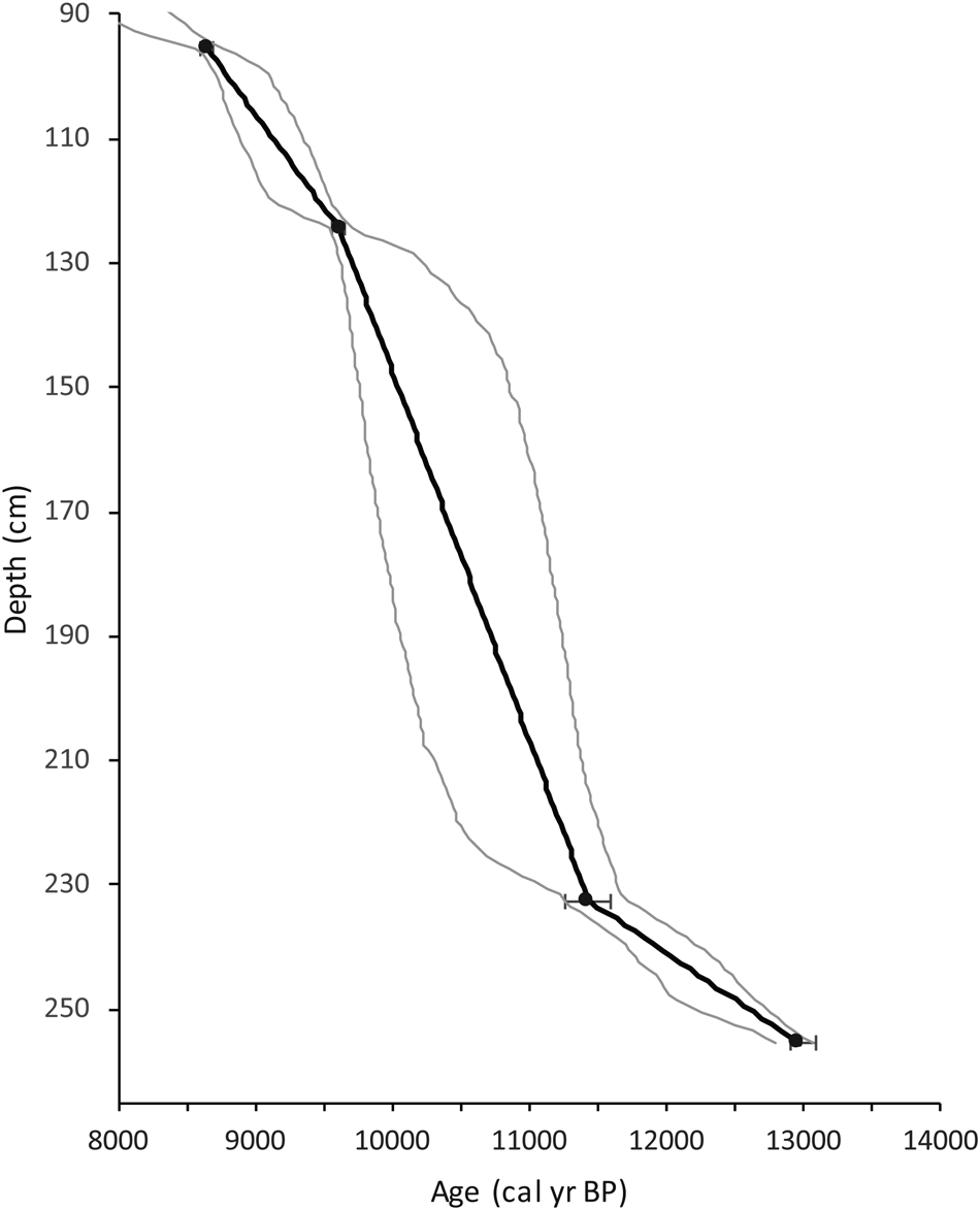
The chronology for the entire 255 cm core was developed by Mandl et al. (Reference Mandl, Shuman, Marsicek and Grigg2016) using 9 14C ages measured with accelerated mass spectrometry (AMS) at the Keck Carbon Cycle AMS Laboratory at the University of California, Irvine. The late-glacial portion of the record is from ca. 90 to 255 cm and contains 4 14C ages (Fig. 2). 14C ages were originally calibrated by Mandl et al. (Reference Mandl, Shuman, Marsicek and Grigg2016) using the IntCal09 calibration data set within the Bchron package in R (Reimer et al., Reference Reimer, Baillie, Bard, Bayliss, Beck, Blackwell, Ramsey, Buck, Burr and Edwards2009; Parnell, Reference Parnell2014). Since this publication, the Bchron package has been updated with the IntCal13 calibration curve (Reimer et al., Reference Reimer, Bard, Bayliss, Beck, Blackwell, Ramsey, Buck, Cheng, Edwards and Friedrich2013). A comparison of the mean age models produced using the two calibration curves shows a maximum offset between samples ages of 43 years and an average offset of 5.5 years. Based on the closeness of the two chronologies and the desire to keep ages consistent between previously published proxies, this study retained the original IntCal09 calibrated ages from Mandl et al. (Reference Mandl, Shuman, Marsicek and Grigg2016).
Calibrated radiocarbon ages plotted as circles and error bars vs. depth. The mean age model (black line) and the range of possible age models between 97.5% and 2.5% (gray lines) values are also shown plotted vs. depth.

The Bchron package was used to calculate age uncertainties for each dated interval and were then interpolated to each 1 cm sample interval throughout the core. The resulting calculated errors for the entire core were then propagated with a Monte Carlo Markov chain, which yielded a population of 10,000 possible age estimates for each sample interval. These data were used to develop a mean age for each sample and the 2.5% and 97.5% quantiles (Fig. 2). From depths of 90 to 130 cm, the range of possible dates between quantiles span an average of 400 years. The lack of ages between 130 and 230 cm and increased radiocarbon and calibration errors result in average age uncertainties of 1000 years. Two dates constrain age uncertainties for the remainder of the record to within an average of 500 years. The mean age model is used to present this record, but all ages should be viewed as an average within a 400–1000 year range of possible ages. These large age uncertainties limit intercore comparisons of specific centennial- to millennial-scale events but do not hinder same-core comparisons between multiple proxies.
Pollen analysis
Subsamples of 1 cm3 at 2–10 cm intervals were sent for pollen processing at the LaCore Facility at the University of Minnesota following standard methods (Faegri and Iversen, Reference Faegri, Iversen, Faegri, Kaland and Krzywinski1989). Microspheres were added to each sample to enable calculation of pollen influx and accumulation rates (Stockmarr, Reference Stockmarr1971). Pollen residues were stored and mounted in silicon oil for examination at magnifications of 400× and 1000×. Taxon identifications were made based on reference manuals (McAndrews et al., Reference McAndrews, Berti and Norris1973; Kapp et al., Reference Kapp, King and Davis2000) and visits to the pollen reference collection at the Harvard Forest, Peachum, MA. Between 300 and 450 pollen grains were identified for each sample. Counts below 350 were limited to those samples with low pollen concentrations (depths >245 cm).
Betula is an important genus at Twin Ponds, and the ability to identify it to the species level facilitates environmental reconstruction. Measurements of Betula pollen grain diameter and pore depth were made following previously described methods (Leopold, Reference Leopold1956; Davis, Reference Davis1958; Ives, Reference Ives1977; Clegg et al., Reference Clegg, Tinner, Gavin and Hu2005). Twenty-five grains from four separate intervals corresponding to peaks in Betula percentages were measured. Pore depth and the ratio of grain diameter to pore depth have both been shown to be effective at differentiating between shrub birch (Betula glandulosa) and paper birch (Betula papyrifera) in herbarium samples from northern North America (Ives, Reference Ives1977; Clegg et al., Reference Clegg, Tinner, Gavin and Hu2005). Differentiation by grain diameter alone has been used for eastern fossil pollen species by Leopold (Reference Leopold1956) and Davis (Reference Davis1958) but has not been systematically tested against modern reference material. For this study, both methods, (1) pore depth and diameter/pore depth and (2) grain diameter alone, were used to distinguish Betula shrub versus tree pollen types.
The modern analog technique (MAT) (Overpeck et al., Reference Overpeck, Webb and Prentice1985) for the quantitative reconstruction of past environments from pollen data was performed using the Analogue package in R (Simpson, Reference Simpson2007) and the North American Pollen Database (Whitmore et al., Reference Whitmore, Gajewski, Sawada, Williams, Shuman, Bartlein, Minckley, Viau, Webb and Shafer2005). Forty-nine eastern- and/or northern-specific species were selected for the analysis (Williams and Shuman, Reference Williams and Shuman2008). For Betula, B. papyrifera pollen-type was combined with other undifferentiated Betula pollen to account for the likely presence of both tree and shrub species. Given the northern location of Twin Ponds and the timing of the record, sites from the modern database from latitudes south of 34.5°N were not included. The first set of MAT analyses identified the closest modern analogs for each fossil sample through the calculation of the dissimilarities (square-chord distances) between each fossil pollen assemblage and the modern data set. Samples with a square-chord distance greater than the 5.0 percentile of the distribution of dissimilarities in the modern data set were classified as no-analog samples. The second set of analyses averaged the climate data from the four to five closest modern analog sites to each fossil sample to reconstruct climate through time. The errors associated with these reconstructions were derived for each climatic variable by adding to/subtracting from the reconstructed fossil value, the residual mean-square error (RMSE) between predicted and observed values in the modern data set. Annual temperature, growing degree days, mean temperature of coldest months, mean temperature of warmest months, and annual and seasonal precipitation totals were all considered.
Ostracode analysis
Ostracode sample preparation and analysis were completed at the Paleolimnology Lab at Kent State University (Engle, Reference Engle2015). One cubic centimeter of sediment was sampled at 1-cm intervals, then the sediment was washed through 150 and 63 μm sieves (100 and 230 mesh). In some cases, the sediment had to first be disaggregated before sieving by treating the sample with 800 ml of hot water and 5 cc of baking soda, followed by cooling to room temperature (Forester, Reference Forester1988). The samples were treated with 2 cc of Calgon® and allowed to sit for 24–48 hours (Forester, Reference Forester1988) and were then washed through the sieves. Once samples were sieved, they were freeze-dried in a Virtis Freezemobile 12ES freeze dryer for ca. 48 hours. The dried samples were then examined under a dissecting microscope at magnifications of 20×–80×. Ostracode shells were picked using a fine-tipped wet paintbrush and were placed on a 60 grid paleontology slide for identification. Identification was based on the extensive ostracode species collection and monograph collection housed in the Geology Department at Kent State. Results are reported as number of ostracod valves counted per gram of dried sediment.
Principal components analysis
To better capture variability across the different proxies through time, principal components analysis (PCA) was performed using a correlation matrix (princomp in R). Before the PCA, the pollen percentage and isotope data were interpolated (approx. in R) to match the higher resolution of the ostracode and LOI data. The variable loadings and sample scores for the first three principal components were examined to identify the most significant patterns of variability across all proxies.
RESULTS
Chronology, LOI, and XRF
The late-glacial chronology was extracted from the age model for the full core (13.6-0 cal ka BP) and is based on four radiocarbon dates from charcoal and/or wood fragments (Mandl et al., Reference Mandl, Shuman, Marsicek and Grigg2016; Fig. 2). Radiocarbon results from sediment younger than 8.0 cal ka BP contain two radiocarbon dates out of chronological order (not used in the age model) and very low sedimentation rates (<0.02 mm/yr) that suggest the reworking of old sediments and a depositional hiatus in a nearshore environment (Mandl et al., Reference Mandl, Shuman, Marsicek and Grigg2016). Because this study does not focus on the period after 9.0 cal ka BP, the age uncertainties associated with this hiatus do not impact our analyses. The sedimentation rate was highest (0.8–0.5 mm/yr) between 13.5 and 11.5 cal ka BP. Sedimentation rates dropped after 11.5 cal ka BP to 0.1–0.3 mm/yr and remained low throughout the rest of the record.
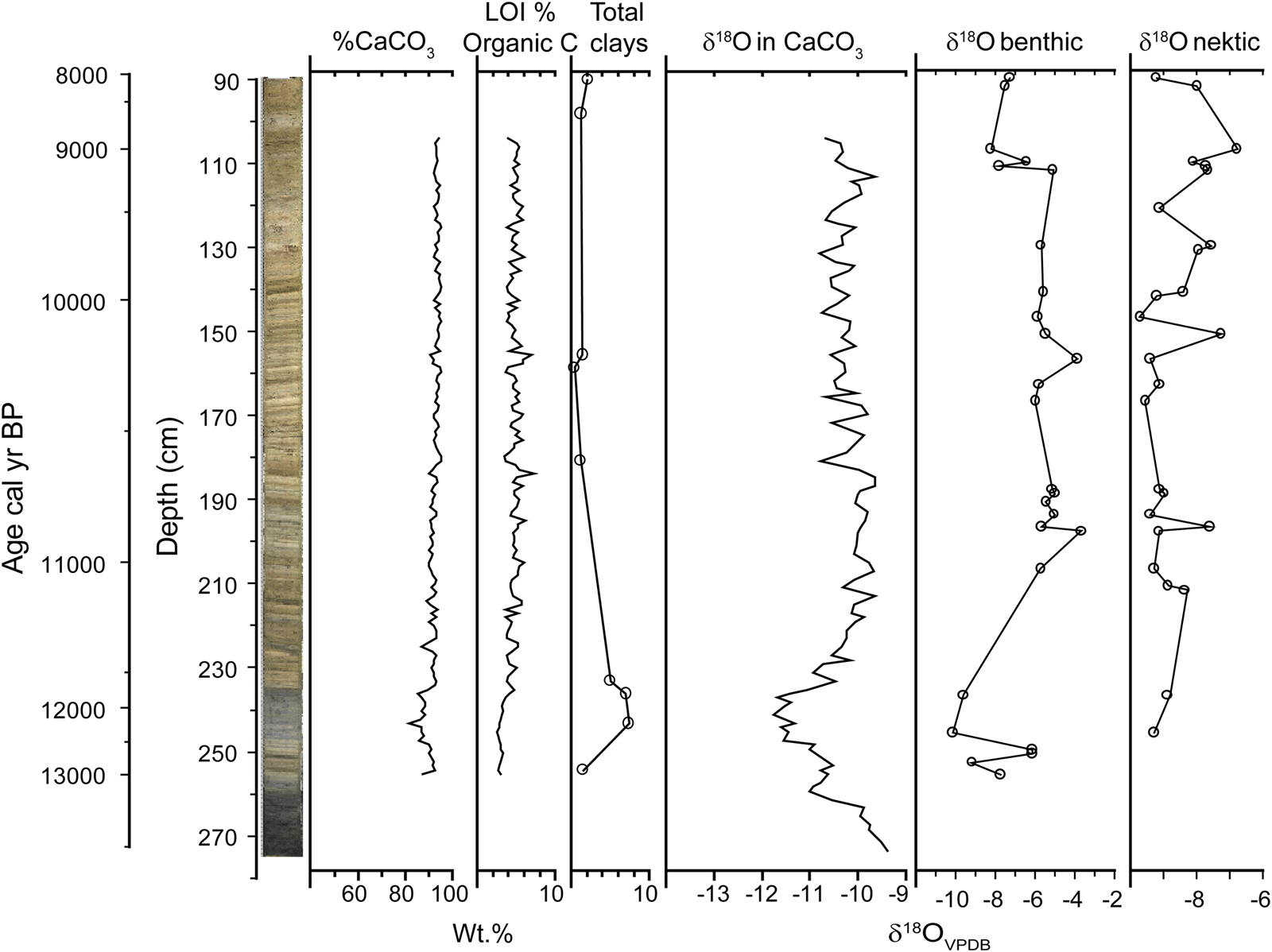
The LOI results from Mandl et al. (Reference Mandl, Shuman, Marsicek and Grigg2016) show the dominance of carbonate sediments throughout the core (Fig. 3). LOI carbonate values range from ca. 81% to 95% and organic carbon values range between 2% and 7%. A period of lower carbonate values (81%–88%) occurred between ca. 12.8 and 11.78 cal ka BP. Organic carbon percentages are low (2%–3%) from 13.5 to 11.8 cal ka BP and then increase slightly to ca. 5%. XRF analysis of select samples reveals the highest weight percentages of clay minerals (4.97%–7.37%) between 12.3 and 11.6 cal ka BP (Fig. 3). The end of this interval of high clay content is poorly constrained by a large sample gap between ca. 232 and 180 cm core depth.
(color online) Core image, loss-on-ignition (LOI) percentages for CaCO3 and organic carbon, percentages of total clays, and δ18O oxygen isotope values for bulk CaCO3 and benthic and nektic ostracodes plotted with a primary axis of depth and age as a secondary axis.

Oxygen isotopes
The full δ18Ocalcite record for Twin Ponds was previously published by Mandl et al. (Reference Mandl, Shuman, Marsicek and Grigg2016) and compared with other δ18O records from the region. δ18Ocalcite values at the base of the core are the highest of the record (−9.34‰) but drop rapidly at 13.3 cal ka BP and remain low until rapidly increasing between 11.7 and 11.2 cal ka BP. The early Holocene portion of the δ18Ocalcite record shows less variability than the preceding late Pleistocene and a broad plateau of δ18Ocalcite values (−9.65‰ to −10.00‰) between 11.2 and 10.6 cal ka BP. The end of the late-glacial record shows a peak centered at 9.3 cal ka BP followed by a steady decline to −11.22‰.
The δ18Obenthic ostracode record is in general agreement with that of the δ18Ocalcite record (Fig. 3). The offset of about 2.00‰ in the benthic ostracode isotope values as compared with that of the bulk carbonate values is due to a vital effect observed in species of the genus Candona (Von Grafenstein et al., Reference Von Grafenstein, Erlernkeuser and Trimborn1999). The lowest values (−10.14‰) of the benthic record occur between ca. 12.4 and 11.8 cal ka BP followed by a rapid increase. Between ca. 11.0 and 9.2 cal ka BP, the benthic values are generally high (−5.97‰ to −3.67‰), with two peaks occurring at 10.9 and 10.3 cal ka BP. The peak at 10.9 cal ka BP overlaps with the high plateau in the δ18Ocalcite values but not with any individual peak. The final increase (−5.09‰) in the benthic record at 9.2 cal ka BP overlaps with the δ18Ocalcite peak centered at 9.3 cal ka BP and is followed by a similar decline to an average of ca. −7.00‰ for the remainder of the record. The δ18Onektic ostracode record begins at ca. 12.4 cal ka BP (Fig. 3). In contrast to the δ18Ocalcite/benthic records, the lowest values (ca. −9.50‰) of the record occur during the early Holocene and are separated by peaks (−7.24‰ to −7.92‰) at 11.1, 10.9, and 10.2 cal ka BP. The record ends with two broad peaks at 9.9–9.5 and 9.2–8.3 cal ka BP. Peaks in the nektic record generally occur when the δ18Ocalcite/benthic records are low and vice versa (Fig. 3).
Pollen data
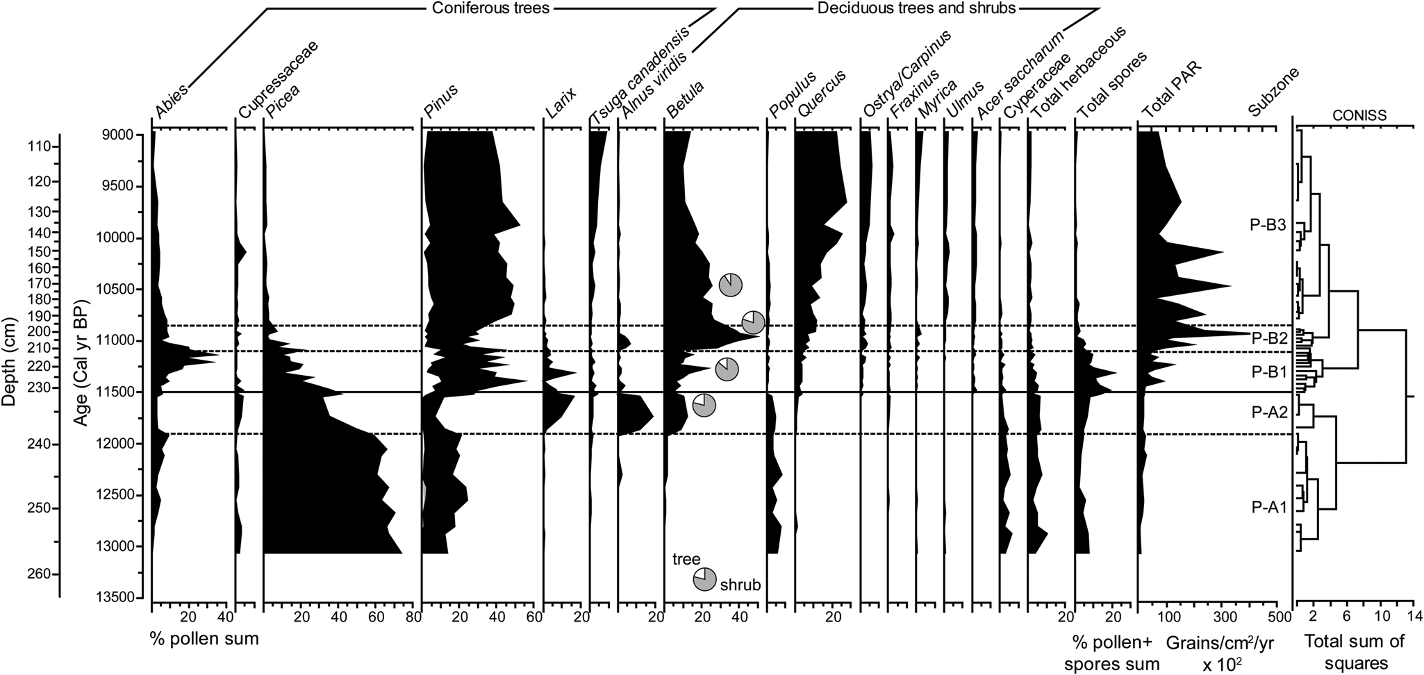
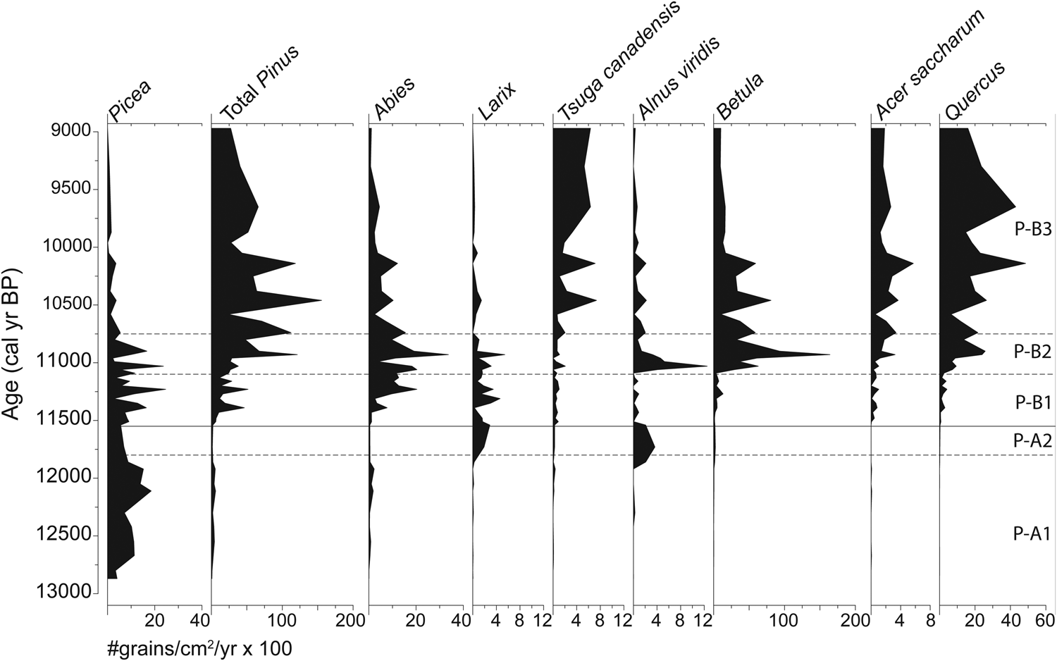
Pollen zones were established based on a stratigraphically constrained cluster analysis on only upland pollen percentages (spores and aquatic pollen were not included) (Grimm, Reference Grimm1987; Fig. 4). The nomenclature for pollen zones follows those established for northeastern North America by Deevey (Reference Deevey1939) and also used for nearby Knob Hill Pond in Marshfield, VT (Oswald and Foster, Reference Oswald and Foster2012). Pollen accumulation rates (PARs) and percentages are shown for major taxa (Figs. 4 and 5).
Pollen percentage diagram for selected taxa with percentages ≥5%. For the Pinus curves: black curve, Pinus undifferentiated; white curve, Pinus strobus; stippled gray curve, Pinus pinus. The small pie charts along the Betula curve show the results of species differentiation at four intervals: gray area, % shrub pollen; white area, % tree pollen. Total pollen accumulation rates, subzones, and the results of CONISS cluster analysis (Grimm, Reference Grimm1987) are also shown.

Pollen accumulation rates for major taxa shown by age with pollen subzones.

Pollen zone A (zone P-A) spans the early part of the record from 13.0 to 11.5 cal ka BP and is characterized by low total PARs of <2000 grains/cm2/yr (Figs. 4 and 5). The pollen percentage record is broken up into two subzones. Subzone P-A1 is dominated by high percentages of Picea (ca. 70%) and smaller amounts of Pinus (20% to 10%), Abies (10% to 5%), and herbaceaous taxa (5%–10%; mostly Cyperaceae). Picea PARs increase (from ca. 500 to 1700 grains/cm2/yr) between 12.8 and 11.8 cal ka BP (Fig. 5). Following the subzone boundary at 11.8 cal ka BP, percentages and PARs of coniferous taxa decrease and Alnus viridis, Betula, and Larix (<2 to ca. 15%) increase. The end of P-A2 shows a brief peak in Picea pollen (50%) and a corresponding decline in A. viridis, Betula, and Larix (≤5%).
The onset of pollen zone B (11.5–9.0 cal ka BP) is marked by an increase in total PARs to >10,000 grains/cm2/year and the continued decline in the dominance of Picea pollen (Figs. 4 and 5). A series of changes in the dominance of arboreal pollen separates zone P-B into three subzones. During subzone P-B1 (11.5–11.1 cal ka BP), Pinus (30%–50%) and Abies (5%–30%) pollen increase, while Picea (10%–25%) and Cyperaceae (<5%) pollen decrease. Larix (5%–15%) and Betula (10%–25%) pollen is also present and peaks ca. 11.3 cal ka BP. Measurements of Betula pollen grains from 11.5 and 11.3 cal ka BP suggest the dominance of shrub Betula, most likely B. glandulosa (Fig. 4), based on published thresholds for pore depth, pore depth:diameter, and grain diameter (Davis, Reference Davis1958; Clegg et al., Reference Clegg, Tinner, Gavin and Hu2005). Subzone P-B1 also shows a noticeable increase in the total number of spores (10%–20% of total pollen and spores). Subzone P-B2 (11.1–10.8 cal ka BP) is dominated by high percentages of Betula pollen (25%–50%) and a decline in coniferous taxa, including Pinus (20%), Abies (5%–10%), and Picea (≤5%). Betula pollen measurements from 11.0 cal ka BP indicate the continued dominance of shrub Betula. Subzone P-B3 (10.8–9.0 cal ka BP) shows a relative stabilization of pollen percentages compared with the previous subzones. P-B3 is dominated by Pinus (40%–50%) but also shows a decline in Betula pollen (still mostly shrub at 10.5 cal ka BP) down to 10% and a corresponding increase in Quercus pollen up to 25%. The diversity of pollen from arboreal taxa increases during subzone P-B3, with the first significant appearances of T. canadensis, Acer, Ostrya/Carpinus, and Ulmus.
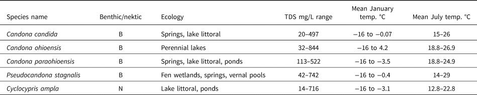
Ecohydrologic significance of common ostracode species in the Twin Ponds record (NANODe, http://www.kent.edu/NANODe; access|ed June 2020; Forester et al., Reference Forester, Smith, Palmer and Curry2005).

The cutoff dissimilarity for close modern analogs for the fossil pollen assemblages was 0.209 square-chord distance, as determined by the 5.0 percentile distribution of dissimilarities in the modern data set. Out of 46 samples, 4 had dissimilarity distances greater than the cutoff and therefore did not have any close modern analogs. Twenty-one samples had less than 5 close modern analogs. The first half of subzone P-B3 (10.8–10.3 cal ka BP) had the largest number of modern analogs and the lowest dissimilarity distances between the fossil samples and the closest modern analogs, while zone P-A had the lowest number of modern analogs and the highest dissimilarity distances. Climate variables were reconstructed for all fossil samples, but given the limited number of modern analogs throughout the record, the MAT results should be viewed as indices of relative change in temperature and precipitation, rather than exact reconstructions. The MAT results for mean temperatures of the warmest (MTWM) and coldest month (MTCO) and total annual precipitation are presented.
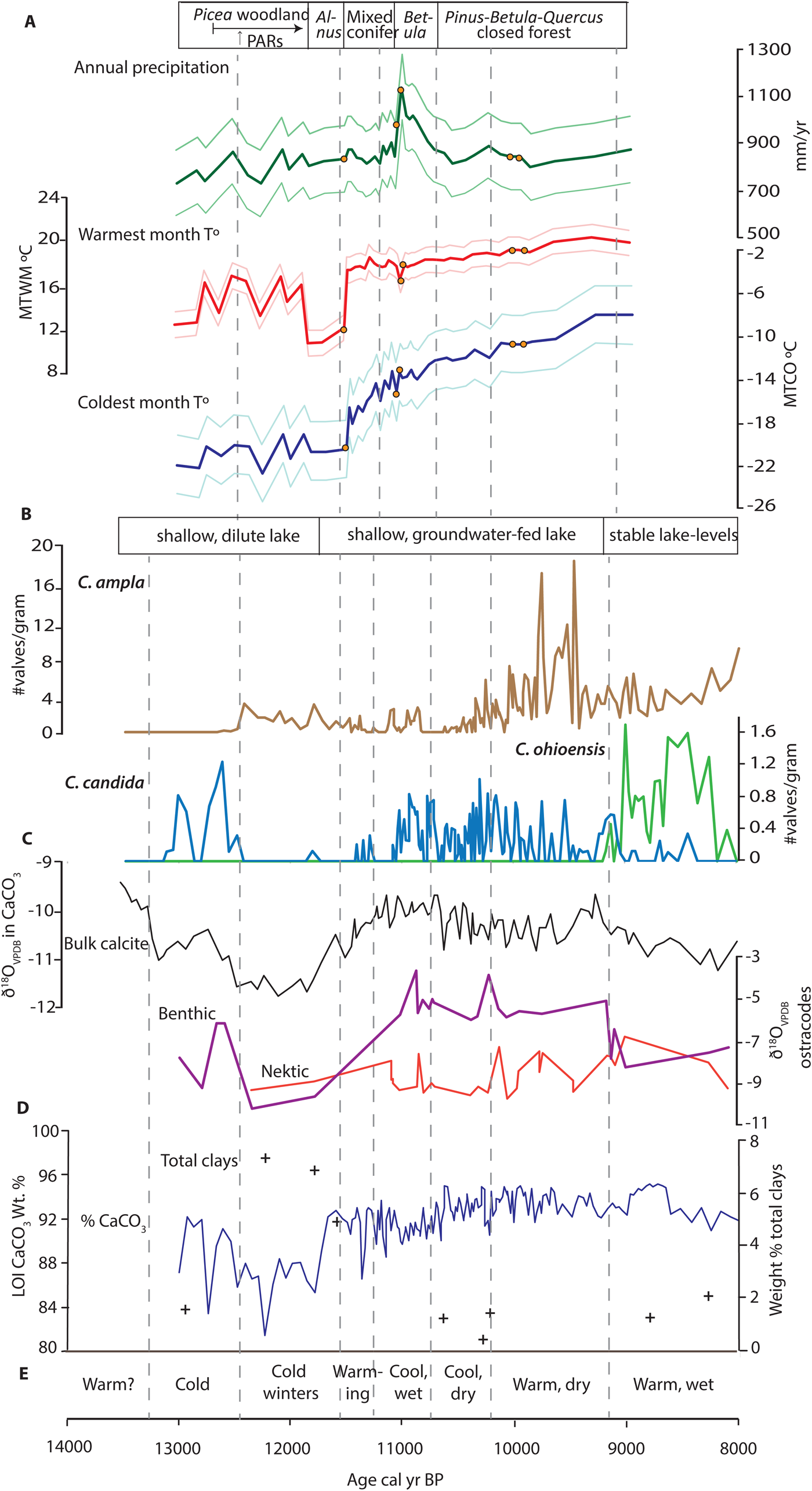
The limited number of modern vegetation analogs found during zone P-A come from the boreal forests and taiga of eastern and midcontinental Canada, which accounts for the generally low reconstructed temperatures (Fig. 6A). The degree of cooling relative to the present was greatest during the winter, with less cooling in the summer. Winter and summer temperatures were highest during zone P-A between 12.6 and 11.9 cal ka BP and reached a low between 11.8 and 11. 6 cal ka BP. The reconstructions for total annual precipitation show the driest conditions of the record occurring during zone P-A before 12.0 cal ka BP (Fig. 6A).
Summary figure of multiproxy environmental and climate variables. Variables are listed under each subheading in order of appearance from the top to bottom of the diagram. Dashed vertical gray lines show the timing of major shifts in the first two principal components (see text and Fig. 9 caption). (A) Vegetation reconstructions from pollen data. Pollen modern analog technique (MAT) reconstructions and residual mean-square error–derived errors for: total annual precipitation in mm/yr (green curves), mean temperature for warmest month (MTWM °C, red curves), and mean temperature for coldest month (MTCO °C, blue curves); orange points mark the four samples that did not have a modern analog with a dissimilarity below the threshold. (B) Hydrologic reconstructions from ostracode data: changes in concentration (no. valves/g) of Cyclocypris ampla (brown curve), Candona candida (light blue curve), and Candona ohioensis (light green curve). (C) Oxygen isotope data: δ18Ocalcite (black curve), δ18Obenthic (purple curve), and δ18Onektic (orange curve). (D) Loss-on-ignition (LOI) percentages of CaCO3 (dark blue curve) and percent total clays (+). (E) Summary of climatic interpretations discussed in the text. (For interpretation of the references to color in this figure legend, the reader is referred to the web version of this article.)

Modern analogs for zone P-B are found in the boreal forests of southeastern Canada and the eastern temperate forest of the NE USA. The temperature reconstructions show a rapid rise in both summer and winter temperatures from 11.7 to 11.5 cal ka BP, followed by a small decline in winter temperatures at 11.5 cal ka BP and a leveling out of summer temperatures. Winter temperatures continue to increase until 11.2 cal ka BP. Between 11.2 and 10.8 cal ka BP, both winter and summer temperatures show more centennial-scale variability but maintain the same general trends, with winter temperatures warming and summer temperatures staying constant. Winter temperatures plateau between 10.8 and 10.2 cal ka BP, followed by warming during both seasons for the remainder of the record (Fig. 6A).
The rapid warming that occurred between zones P-A and P-B was accompanied by a moderate increase in total annual precipitation, although conditions still remained drier than present (Fig. 6A). One exception to generally dry conditions was a significant increase in total annual precipitation between 11.1 and 10.8 cal ka BP. This increase in moisture in the MAT is driven by high percentages of Betula that currently occur in cool, moist habitats, such as wetlands and damp forests (Flora of North America Editorial Committee, 1997). Following this interval, annual precipitation decreases to pre-Holocene levels (Fig. 6A).
Ostracode data
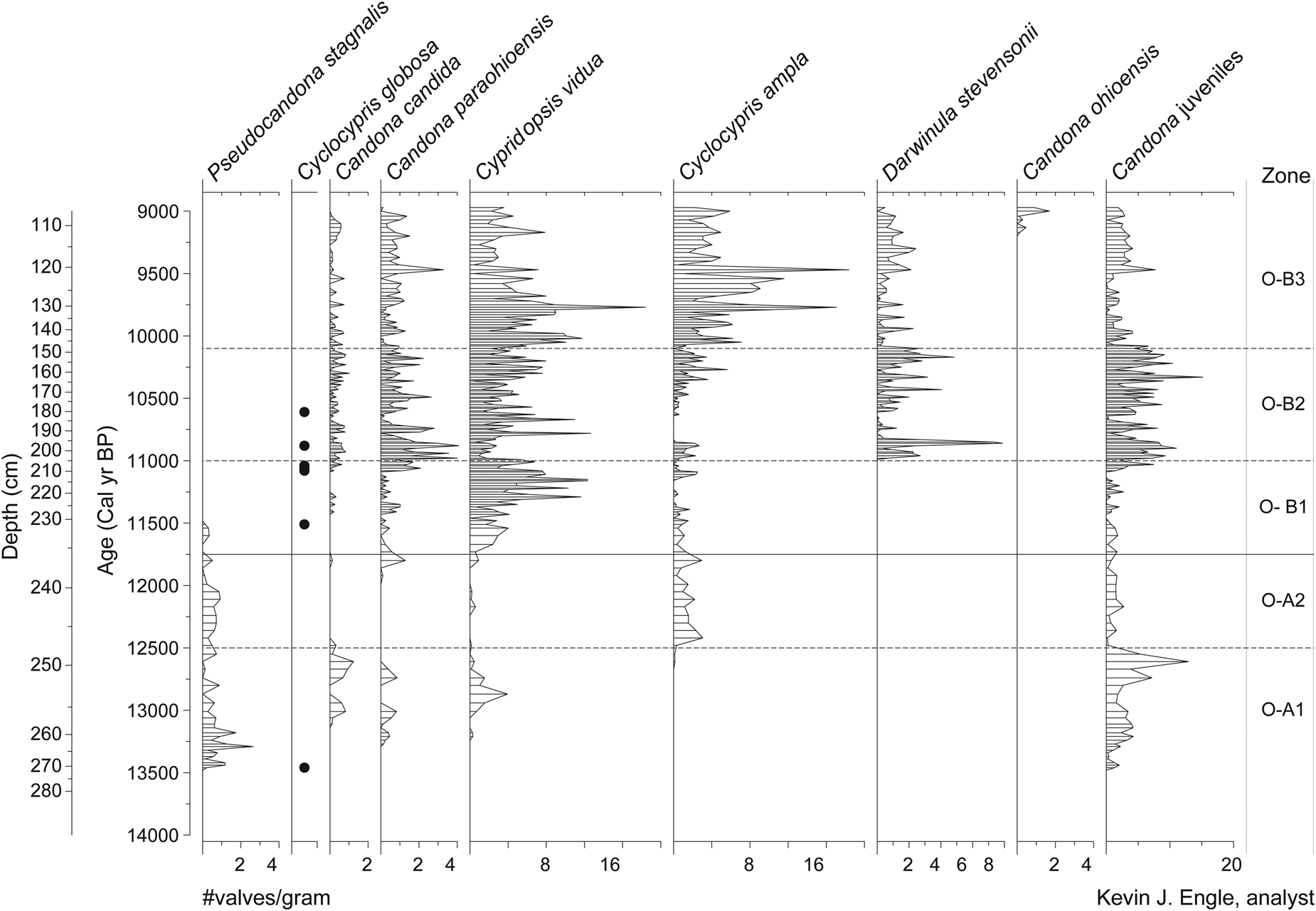
Ostracode (O) zones show close alliance with the pollen zonation (Fig. 7). Overall, the species in this record are cold-tolerant fauna, and most of these species are in the region today, occupying the forested Great Lakes, northern New England, and the Canadian eastern forests (Table 1). One exception is the presence of Cyclocypris globosa, a nektonic species found exclusively in the Arctic today (www.neotomadb.org. Accessed June 2020). This species appears sporadically and in very low numbers in the Twin Ponds core between 13.0 and 10.5 cal ka BP. Zone O-A (13.5–11.8 cal ka BP) is characterized by generally low concentrations of adult ostracodes (<4 valves/g) and the dominant presence of Pseudocandona stagnalis. Subzone O-A1 (13.5–12.5 cal ka BP) begins with the highest concentrations of P. stagnalis (1–3 valves/g) and the rare appearance of C. globosa. During the latter part of this subzone, small peaks in Candona candida (1–2 valves/g) and Candona paraohioensis (0.5–1.0 valves/g) are separated by an increase in Cypridopsis vidua (4 valves/g). Subzone O-A2 (12.5–11.8 cal ka BP) is marked by the absence of C. candida, C. vidua, and C. globosa, the arrival of Cyclocypris ampla (1–2 valves/g), and the continued presence of low concentrations (0.5–1.0 valves/g) of P. stagnalis.
Ostracode concentration diagram (no. valves/gram) plotted by age (Engle, Reference Engle2015). Horizontal bars show intervals sampled. Black dots along the Cyclocypris globosa curve represents its presence.

Ostracode zone B (11.8–9.0 cal ka BP) shows a general increase in the concentrations of adult ostracodes (up to 15 valves/g) and increased species diversity (Fig. 7). Pseudocandona stagnalis disappears at the start of zone O-B and does not return for the remainder of the core, while all other species show a marked increase from the previous zone. Subzone O-B1 (11.8–11.0 cal ka BP) is dominated by C. vidua (5–15 valves/g) and lesser amounts (<2 valves/g) of C. paraohioensis and C. ampla. Subzone O-B2 (11.0–10.10 cal ka BP) is marked by a decrease in C. vidua (to about 4 valves/g), an increase in C. paraohioensis (up to 4 valves/g), and the first appearance of Darwinula stevensoni (ca. 4 valves/g). Candona candida and C. globosa are also present in this subzone in low concentrations (≤1 valve/g). The final O-subzone (O-B3; 10.1–9.0 cal ka BP) is characterized by increased concentrations of both C. vidua and C. ampla, the first appearance of Candona ohioensis at the top of the subzone, and continued low concentrations of all other species from the previous subzone, with the exception of C. globosa, which disappears for the remainder of the record.
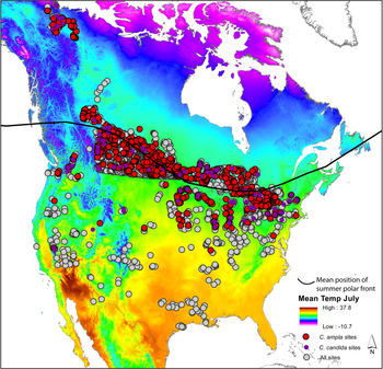
The North American Non-Marine Ostracode Data Project (NANODe, http://www.kent.edu/NANODe. Accessed June 2020; Forester et al., Reference Forester, Smith, Palmer and Curry2005) and the Canadian Museum of Nature–Delorme Ostracoda surface samples data sets (Delorme, Reference Delorme1969; Delorme et al., Reference Delorme, Zoltai and Kalas1977; Delorme and Zoltai, Reference Delorme and Zoltai1984; Forester et al., Reference Forester, Delorme, Ager, David and Peterson1989; Curry and Delorme, Reference Curry and Delorme2003) were used to analyze the environmental significance of the fossil assemblages (www.neotomadb.org). Zone O-A is primarily defined by the occurrence of P. stagnalis, which is the only ostracode present throughout the entire zone and is hydrologically significant in that its preferred habitat is low in total dissolved solids (TDS as low as 42 mg/L) and it is found in ephemeral fens and shallow ponds with aquatic plants with calcium, bicarbonate, and carbonate as the dominant major ions. The rare appearance of the nektonic C. globosa at the start of the subzone O-A1 suggests the early influence of polar air. Candona candida is present between 13.2 and 12.5 cal ka BP and is a northern species with a current southern biogeographic extent that traces the summer position of the polar front (Fig. 8). The presence of C. candida between 13.2 and 12.5 cal ka BP suggests that the position of the summer polar front was at or south of Twin Ponds and implies cool summer air and water temperatures. Candona candida is replaced by C. ampla at the base of subzone O-A2 at ca. 12.5 cal ka. Cyclocypris ampla is also a northern species and has a biogeographic extent similar to that of C. candida, and the two species co-occur in most samples later in the core between 11.4 and 8.5 cal ka BP. However, the modern spatial distribution of the two species shows that C. ampla has a slightly wider southern range at low-elevation sites relative to C. candida (Fig. 8). Thus, this mid-YD shift may suggest a shift to warmer summers.
Map of modern ostracode sites from the North American Non-Marine Ostracode Data Project (NANODe, http://www.kent.edu/NANODe; Forester et al., Reference Forester, Smith, Palmer and Curry2005) and the Canadian Museum of Nature–Delorme Ostracoda surface samples data sets (Delorme, Reference Delorme1969; Delorme et al., Reference Delorme, Zoltai and Kalas1977; Delorme and Zoltai, Reference Delorme and Zoltai1984; Forester et al., Reference Forester, Delorme, Ager, David and Peterson1989; Curry and Delorme, Reference Curry and Delorme2003). Gray circles show the location of all sites from the two data sets; red circles show the sites where Cyclocypris ampla has been found; and purple circles show the sites where Candona candida has been found. Base map shows average July surface temperatures in °C (data from PRISM Climate Group, Oregon State University, http://prism.oregonstate.edu, created November 15, 2020) and black arrow shows the average position of the summer polar front. (For interpretation of the references to color in this figure legend, the reader is referred to the web version of this article.)

The transition to zone O-B is marked by the disappearance of P. stagnalis from the record at 11.5 cal ka BP and the rise in the abundance of littoral-zone swimmers such as C. vidua and benthic C. paraohioensis (Fig. 7). This shift in taxa suggests an increase in groundwater flow into the shallow lake/wetland with TDS > ca.115 mg/L. The increase in D. stevensoni at 11.0 cal ka BP is another indicator of the increasing importance of groundwater into the pond, as this species is associated with interstitial habitats in groundwater-fed littoral zones. The continued presence of C. candida and the rare appearance of C. globosa between 11.5 and 10.5 cal ka BP implies that the position of the summer polar front periodically shifted south of the latitude of Twin Ponds.
The increase in the nektic swimmers C. ampla and C. vidua at the base of subzone O-B3 likely reflects increased productivity in the littoral zone resulting from warmer summers and this is reflected in their isotopic values, which stay relatively constant and isotopically lower than the benthic species (Figs. 3 and 7). The appearance of C. ohioensis in O-B3, at about 9.3 cal ka BP, marks the establishment of a permanent lake (perennial). Candona ohioensis occurs in permanent freshwater lakes in a relatively narrow band in the forested Great Lakes region and the NE USA, and north to about 55° latitude (www.neotomoadb.org). This species has a life span of about a year, reaching adulthood in the winter months and, in the north, under the ice (Ito and Forester, Reference Ito and Forester2017). Its previous absence and the affinity of earlier assemblages to shallow lake/wetland spring environments all suggest that water levels became more stable at the higher end of its previous range. Higher year-round water levels imply an increase in effective moisture and some combination of increased precipitation or less evaporation. An alternative or additional explanation is a reduction in the thickness of ice cover. The grounding of thick winter ice in the littoral zones before this time could have prevented the survival of C. ohioensis, which needs permanent water; thus, its appearance may also mark a transition to warmer, shorter winters.
Multiproxy PCA
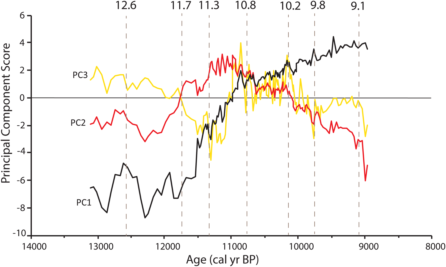
The first three components of the principal components analysis explain 61% of the variance in the interpolated multiproxy data set (Fig. 9). The first principal component (PC1) captures 41% of the variance in the record and reflects the major differences between the late Pleistocene and the early Holocene. Negative scores for PC1 from 13.5 to 11.0 cal ka BP indicate relatively high percentages of Picea, Cyperaceae, and total herbaceous pollen types and high concentrations of the ostracode P. stagnalis. Compared with modern vegetation and ostracode assemblages, these fossil assemblages suggest a climate colder than at present. Positive PC1 scores represent high bulk δ18O, CaCO3, organic carbon, deciduous arboreal taxa, Pinus, and all other ostracode taxa (except P. stagnalis) and collectively indicate a warmer climate relative to negative PC1 scores and an increase in groundwater discharge into Twin Ponds. PC1 scores rise rapidly between 11.5 and 10.8 cal ka BP and then more gradually for the remainder of the record. The steadily increasing trend in PC1 scores is briefly interrupted between 10.9 and 10.6 cal ka BP by a general flattening of the curve slope.
(color online) Principal component scores for principal component 1 (PC1, black curve), principal component 2 (PC2, red curve), and principal component 3 (PC3, yellow curve) plotted by age. Thin horizontal black line marks 0; values above or below this line show intervals that are most strongly aligned with the variation represented by each PC. Dashed vertical gray lines show the timing of major changes in PC scores (>1 PC score between samples) in two or more PCs. (For interpretation of the references to color in this figure legend, the reader is referred to the web version of this article.)

The second principal component (PC2) accounts for 11.5% of the variance within the multiproxy record (Fig. 9). Positive PC2 scores from 11.3 to 10.7 cal ka BP represent a transitional set of proxies between the late Pleistocene and early Holocene and are dominated by high positive loadings of Abies and Betula pollen and bulk δ18O. The lowest negative PC2 scores occur at the very end of the record and reflect the increased importance of T. canadensis and Myrica pollen and the ostracodes C. ohioensis and C. ampla. PC2 also reflects a shift in proxies between 12.5 and 11.8 cal ka BP that is primarily driven by an increase in C. ampla. The third principal component (PC3) further defines the high degree of variance (8.5%) that occurs in the middle and early parts of the record (Fig. 9). High PC3 scores are driven by increases in the ostracodes C. candida, C. paraohioensis, and D. stevensoni and in Betula pollen. The highest PC3 scores occur between 11.0 and 10.0 cal ka BP. The lowest PC3 scores occur between 11.8 and 11.0 cal ka BP and at the end of the record and represent increases in Abies, Larix, total spores, and C. vidua.
Collectively, the first three PC scores show low variability during the late Pleistocene portion of the record (<11.7 cal ka BP) (Fig. 9). The largest changes during this time occur at ca. 12.6 cal ka BP in PC1 and PC2. The early Holocene from 11.7 to 9.8 cal ka BP shows the largest amount of variability in PCs, beginning with shifts in all PCs between 11.7 and 11.5 cal BP. Large fluctuations in PC2 and PC3 continue until 10.8 cal ka BP, with major shifts at 11.2 and 10.8 cal ka BP. The latter third of the record (10.8–9.0 cal ka BP) shows less variability than the preceding interval, with smaller shifts in PC2 and PC3 at 10.2, 9.8, and 9.1 cal ka BP (Fig. 9). These intervals of increased multiproxy change are used in Figure 6 to summarize the multiproxy climatic signal.
DISCUSSION
Late Pleistocene (13.5–11.7 cal ka BP)
The pre-YD record from Twin Ponds is limited because of low concentrations of both pollen and ostracodes (Figs. 4, 5, and 7). High δ18Ocalcite values at the beginning of the record may reflect warm air temperatures associated with the end of the Bølling-Allerød warm interval but may also indicate changes in moisture source area and seasonality (Fig. 6C). A consistent shift at the start of the YD is not apparent in any of the first three principal components and points to a complex climate signal across proxies (Fig. 9). The clearest signal of change during the YD comes from the δ18Ocalcite/benthic values and CaCO3 percentages, which show a decline between ca. 12.8 and 11.6 cal ka BP (Fig. 6C and D). Several samples from this interval also show higher percentages of total clay minerals. Low δ18O calcite and benthic values during the YD could reflect cold air temperatures, less effective moisture, a more northern moisture source area, or an increase in the proportion of winter to summer precipitation (Bowen and Revenaugh, Reference Bowen and Revenaugh2003). The associated decline in CaCO3 percentages and increase in clay content suggest either an increase in erosion into the lake or colder summer water temperatures that caused an increase in the solubility of CaCO3, leading to less dilution of clays. Collectively, these data imply that the relatively large negative excursion in δ18Ocalcite/benthic values may be explained by colder air temperatures or an increase in the proportion of winter precipitation leading to more snowmelt and surface erosion.
The predominance of Picea pollen in the late Pleistocene results in uniformly high pollen percentages throughout the YD until 11.8 cal ka BP. However, an increase in Picea PARs between ca. 12.8 and 11.8 ka cal BP may have a climatic significance (Figs. 5 and 6). Increased PARs result from either an expansion of Picea on the surrounding landscape and/or an increase in the rate of pollen transport into the pond via stream inflow and/or wind. Picea is a cold-adapted species, and its expansion at Twin Ponds during the YD is consistent with the continuation of cold conditions (Fig. 6A). The lack of a pre-YD warm signal from the pollen record may reflect the early stages of ecological succession in central Vermont at the onset of the YD, as indicated by the low diversity of taxa and PARs. Deglaciation did not occur in central Vermont until 14.5–14.0 cal ka BP (Ridge et al., Reference Ridge, Balco, Bayless, Beck, Carter, Dean, Voytek and Wei2012) and perhaps later (13.8 cal ka BP) in the nearby Winooski River valley (Larsen, Reference Larsen2001). Very low PARs in the early part of the record suggest that Twin Ponds had not yet developed a productive and diverse forest community despite evidence from high δ18Ocalcite values for potentially warmer pre-YD atmospheric conditions. YD cooling would have allowed for the continued expansion of cold-adapted, early-successional Picea. Alternatively, or additionally, increased Picea PARs could have resulted from an increase in the transport of pollen into the pond via surface runoff or wind. Increased surface runoff into the pond from winter snowmelt is consistent with low δ18O values and increased clay content.
The ostracode record shows a brief increase in cold-adapted, groundwater-adapted taxa (C. candida and C. paraohioensis) at 12.8 cal ka BP that may indicate the onset of YD cooling (Figs. 6B and 7). However, at 12.6 cal ka BP, these taxa are replaced by P. stagnalis, which persists until 11.8 cal ka BP and suggests that for most of the YD, Twin Ponds was a shallow pond or wetland with low TDS (Figs. 6B and 7). Low TDS during the YD is consistent with evidence from the other proxies for an increase in the influx of snowmelt into the pond. Candona candida and C. ampla are also present during the YD, although at different times (Fig. 6B). While both are northern species with a southern limit that is close to the position of the summer polar front, C. ampla shows more tolerance for warmer summers (Fig. 8), and the shift between the two species at 12.6 cal ka BP may indicate warmer summer temperatures. This interpretation is supported by a higher pollen MAT summer temperature between 12.6 and 11.9 cal ka BP (Fig. 6A); however, because of a lack of modern analogs for this interval, comparisons of the fossil reconstructions to the modern range of temperatures for these two ostracode species is not feasible.
There is evidence for a final cool interval at the end of the YD (11.8–11.6 cal ka BP) from several proxies, as shown by a decline in PC1 at 11.8 cal ka BP (Fig. 9). δ18Ocalcite values and percentages of CaCO3 both decline at 11.8 cal ka BP and then begin a steady rise (Fig. 6C and D). These changes occur alongside a decline in Picea pollen (% and PARs) and increase in A. viridis and shrub Betula pollen (Figs. 4 and 5). This shift in assemblages indicates the development of a shrub tundra in subzone P-A2 (11.8–11.6 cal ka BP) that results in the lowest MAT temperatures of the record (Fig. 6A). However, the pollen-inferred cooling is of longer duration than the cooling indicated by the other proxies (Fig. 6). A similar expansion of A. viridis at the expense of Picea has been identified at high-elevation sites in New Hampshire and New York during and just after the YD and is attributed to increased snowfall and exposure of minerogenic soils related to YD cooling (Jackson, Reference Jackson1989; Spear, Reference Spear1989). The duration of the pollen-inferred cooling beyond that shown by the other proxies from Twin Ponds may be explained by the rapid rise in atmospheric CO2 that occurred throughout the YD (Monnin et al., Reference Monnin, Indermühle, Dällenbach, Flückiger, Stauffer, Stocker, Raynaud and Barnola2001). Increased atmospheric CO2 results in greater plant water-use efficiency and would have allowed less-xeric, cold-deciduous taxa such as Betula and Alnus to expand at the expense of coniferous taxa (Polley et al., Reference Polley, Johnson, Marinot and Mayeux1993; Cowling and Sykes, Reference Cowling and Sykes1999; Williams et al., Reference Williams, Webb, Shurman and Bartlein2000). This explanation may also apply to the widespread occurrence of Alnus during the YD previously noted throughout the NE USA and adjacent Canada (Mayle et al., Reference Mayle, Levesque and Cwynar1993).
In summary, the multiproxy data from Twin Ponds suggest that the YD was generally cold and dry with a greater portion of the cooling occurring in the winter (Fig. 6). There is also evidence from across proxies for an increase in surface runoff from snowmelt. The Twin Ponds YD record is similar to records from southern Ontario that show little change in pollen percentages but a notable decrease in δ18O values and an increase in erosional elements (Yu and Eicher, Reference Yu and Eicher1998). Increased surface runoff from snowmelt during the YD implies colder or wetter winters leading to increased snow accumulation followed by subsequent summer snowmelt. Strong winter cooling at Twin Ponds is supported by the pollen MAT temperature reconstructions (Fig. 6A) and is consistent with the expansion of sea ice and colder SSTs in the North Atlantic (Ruddiman and McIntyre, Reference Ruddiman and McIntyre1981; Rind et al., Reference Rind, Peteet, Broecker, McIntyre and Ruddiman1986; Pearce et al., Reference Pearce, Seidenkrantz, Kuijpers, Massé, Reynisson and Kristiansen2013). Less YD cooling during the summer at Twin Ponds is evident in the MAT temperature reconstructions (Fig. 6a) and has also been noted in other inland records from northern New England, while coastal records from Maine and maritime Canada suggest year-round cooling (Cwynar and Levesque, Reference Cwynar and Levesque1995; Cwynar and Spear, Reference Cwynar and Spear2001; Shuman et al., Reference Shuman, Webb, Bartlein and Williams2002b). These paleoclimatic observations are supported by model simulations that show the strongest YD cooling in North America during the winter time along the northeastern coastline and steep east–west summer temperatures gradients driven by cold SSTs and summertime heating of the interior continent by increasing summer insolation values (Rind et al., Reference Rind, Peteet, Broecker, McIntyre and Ruddiman1986; Fawcett et al., Reference Fawcett, Ágústsdóttir, Alley and Shuman1997; Manabe and Stouffer, Reference Manabe and Stouffer1997).
Although evidence for increased moisture during the YD has been observed in central New York and multiple locations in the Midwest (Dwyer et al., Reference Dwyer, Mullins and Good1996; Gonzales and Grimm, Reference Gonzales and Grimm2009; Voelker et al., Reference Voelker, Stambaugh, Guyette, Feng, Grimley, Leavitt, Panyushkina, Grimm, Marsicek and Shuman2015) and would also explain the observed increase in surface runoff from snowmelt at Twin Ponds, the pollen MAT annual precipitation reconstructions show consistently dry conditions both before and during the YD (Fig. 6A). This is further evidence that increased seasonality and not increased precipitation is the likely explanation for the observed increase in surface runoff during the YD. These results are supported by climate simulations of hydroclimate variability in North America that indicate increased moisture in the Midwest and decreased moisture in Vermont during the YD (Renssen et al., Reference Renssen, Goosse, Roche and Seppä2018; Lora and Ibarra, Reference Lora and Ibarra2019).
Early Holocene (11.7–9.0 cal ka BP)
The end of the YD is clearly marked by a steady rise in PC1 and PC2 at ca. 11.7 cal ka BP and reflects the increase in δ18Ocalcite/benthic values, percentages of CaCO3, and groundwater-adapted ostracodes and C. vidua (Fig. 9). These isotopic changes imply warmer air temperatures, a reduction in the proportion of winter precipitation flowing into the lake, or a southern shift in moisture source area (Bowen and Revenaugh, Reference Bowen and Revenaugh2003). The shift in ostracode assemblages suggests a greater proportion of groundwater influx and the expansion of productive shallow littoral environments. The pollen MAT temperature reconstructions match these trends, with a rapid increase beginning at 11.6 cal ka BP (Fig. 6A). Collectively, these results point toward a moderation in air and water temperatures and are consistent with the rapid loss of sea ice off Newfoundland at 11.7 cal ka BP (Pearce et al., Reference Pearce, Seidenkrantz, Kuijpers, Massé, Reynisson and Kristiansen2013).
The pollen record shows a sequence of centennial-scale changes during pollen subzones P-B1 and P-B2 (11.6–10.8 cal yr BP) that indicate a rapid sequence of vegetation change from mixed conifer forest to shrub birch to pine/oak forest (Figs. 4 and 5). A pollen record from nearby Knob Hill Pond in Marshfield, VT (Oswald and Foster, Reference Oswald and Foster2012) shows the same sequence and general timing of vegetation changes, indicating that these changes were regional in extent. Similar rapid sequences of vegetation change following the end of the YD are common (Birks and Ammann, Reference Birks and Ammann2000; Williams et al., Reference Williams, Post, Cwynar, Lotter and Levesque2002) and could be a response to a combination of factors, including variable rates of plant migration, soil development, landscape instability, or the continuation of a rapidly changing climate (Birks and Birks, Reference Birks and Birks1980). At Twin Ponds, rapid vegetation change coincides with the continuation of climatic instability, as inferred from the other proxies.
Superimposed on the early Holocene warming trend is evidence for brief cooling at ca. 11.5 cal ka BP. All three PCs show a decline at 11.5 cal ka BP and reflect the multiproxy nature of this event, including decreases in δ18Ocalcite values and percentages of CaCO3. (Figs. 6 and 9). Additionally, increases in Picea pollen (% and PARs) at 11.5 cal ka BP result in a brief decline in MAT-reconstructed winter temperatures (Fig. 6A). The timing and duration of this cold period is similar to a brief cold event identified in Ontario and New Jersey around 11.3 cal ka BP (Anderson et al., Reference Anderson, Mullins and Ito1997; Yu and Eicher, Reference Yu and Eicher1998) and evidence for an interruption in warming at the end of the YD in Nova Scotia (Vincent and Cwynar, Reference Vincent and Cwynar2016). Yu and Eicher (Reference Yu and Eicher1998) correlate the timing of this cold interval with the Preboreal Oscillation, a cold, wet period identified in Greenland ice cores (Lehman and Keigwin, Reference Lehman and Keigwin1992; Rasmussen et al., Reference Rasmussen, Vinther, Clausen and Andersen2007) and in northwest Europe between 11.3 and 11.15 ka cal BP (Björck et al., Reference Björck, Kromer, Johnsen, Bennike, Hammarlund, Lemdahl, Possnert, Rasmussen, Wohlfarth and Hammer1996, Reference Björck, Rundgren, Ingolfsson and Funder1997). The cool interval from Twin Ponds predates the Preboreal Oscillation, and the short duration and timing of this event during several 14C plateaus, in addition to uncertainties in the Twin Ponds age model, limits precise intersite correlation (Björck et al., Reference Björck, Rundgren, Ingolfsson and Funder1997).
A broad peak in PC2 between 11.3 and 10.8 ka cal BP reflects a plateau in the bulk and δ18Ocalcite/benthic values, a low in the δ18Onektic values, a small decrease in percentages of CaCO3, an increase in the groundwater-adapted ostracodes C. paraohioensis and D. stevensoni, and high percentages/PARs of Betula pollen (Figs. 6 and 9). The increase in Betula pollen results in the highest MAT-reconstructed annual precipitation of the record and a decrease in temperatures around 11.0 cal ka BP (Fig. 6A). Lower δ18Onektic values and percentages CaCO3 also suggest summer cooling during this time (Fig. 6C and D). The increase in groundwater-adapted ostracodes and plateau in δ18Ocalcite/benthic values can be explained by an increase in shallow-groundwater discharge into the lake resulting from increased summer or southern-sourced precipitation. Alternatively, high δ18Ocalcite/benthic values could reflect increased shallow-groundwater discharge of more 18O-enriched groundwater and may not require a seasonal or geographic shift in precipitation sources. A multiproxy study from Minnesota noted a similar discrepancy, with low δ18O values corresponding to drought (Donovan et al., Reference Donovan, Smith, Ito, Engstrom and Panek2002; Smith et al., Reference Smith, Donovan, Ito and Engstrom1997, Reference Smith, Donovan, Ito, Engstrom and Panek2002). This apparent discrepancy was attributed to a decrease in the size of groundwater recharge zones and groundwater residence time during dry conditions, which resulted in the influx of less evolved groundwater into the lake. Thus, enriched δ18O values in groundwater at Twin Ponds during wet conditions may similarly be explained by an increase in the area of shallow recharge zones and a longer residence time leading to higher δ18O values.
The plateau in δ18O values centered around 11.0 cal ka BP at Twin Ponds was previously described by Mandl et al. (Reference Mandl, Shuman, Marsicek and Grigg2016) and is also seen in the isotope record from Fayetteville Green Lake, NY, where it was attributed to an expanded trough in the polar jet stream (Kirby et al., Reference Kirby, Patterson, Mullins and Burnett2002a, Reference Kirby, Mullins, Patterson and Burnett2002b). The more meridional flow associated with this trough would have brought storms from more southerly locations into the NE USA and would have caused an increase in high δ18O values. Kirby et al. (Reference Kirby, Patterson, Mullins and Burnett2002a) suggest that an expanded trough resulted from an increase in land–ocean temperature differences between the North Atlantic and North America. Steeper east–west temperature gradients are consistent with a stronger post-YD Atlantic Meridional Overturning Circulation and the lingering presence of the Laurentide Ice Sheet over Canada (Kirby et al., Reference Kirby, Patterson, Mullins and Burnett2002a). The evidence for increased precipitation from Twin Ponds does not contradict this interpretation but does provide an alternative explanation for high δ18Ocalcite/benthic values. Low δ18Onektic values and pollen-inferred temperatures from Twin Ponds also suggest that summer air and water temperatures were likely cooler. Ellis et al. (Reference Ellis, Mullins and Patterson2004) also document cooling at Seneca Lake, NY, during the post-YD between 11.6 and 10.3 cal ka BP.
PC2 scores decline at ca. 10.8 cal ka BP and mark the decrease in Betula pollen and δ18Ocalcite/benthic values and the increasing importance of the ostracode C. ampla (Figs. 6 and 9). PC1 scores remain level with minor fluctuations until 10.6 cal ka BP and then rise steadily for the remainder of the record (Fig. 9). Increasing PC1 scores reflect decreasing Picea pollen, increasing Pinus and deciduous arboreal pollen, and increasing CaCO3 percentages. The δ18Onektic values are generally low during this time but show more variability, with peaks centered on 10.9, 10.2, and 9.8 cal ka BP, and suggest cool but fluctuating summer water temperatures (Fig. 6C). The pollen MAT indicates a decline in precipitation as Betula pollen decreases at the expense of Pinus pollen (Fig. 6A). These data are consistent with the interpretation that a reduction in δ18Ocalcite/benthic values represents a decrease in the source area of shallow-groundwater flow due to drier conditions. The pollen MAT temperature indices show a plateau in warming between 10.8 and 10.2 cal ka BP (Fig. 6A). The continued presence of C. candida and appearances of C. globosa until 10.5 cal ka BP also suggest the continuation of cool conditions (Figs. 6b and 7).
PC2 and PC3 scores decrease after 10.2 cal ka BP and reflect a decline in Betula pollen and the groundwater-adapted ostracodes C. paraohioensis and D. stevensonii (Fig. 9). The pollen MAT temperatures indices both steadily increase from 10.2 cal ka BP to the end of the record, while precipitation remains low (Fig. 6A). A decrease in δ18Ocalcite/benthic values and CaCO3 percentages and a peak in C. ampla at ca. 9.6 cal ka BP may represent a brief cold interval, but there were no significant changes in the pollen, which could be a reflection of a coarser sampling interval after 10.0 cal ka BP (Fig. 6). The record ends with a final shift in isotopes and ostracodes. A peak in δ18Ocalcite/benthic values between 9.4 and 9.2 cal ka BP overlaps with a small increase in CaCO3 and the appearance of the ostracode C. ohioensis (Fig. 6). After 9.2 cal ka BP, δ18Ocalcite/benthic values decline, while δ18Onektic values and the abundance of the ostracode C. ohioensis increase (Fig. 6). Candona ohioensis is an important indicator of permanent open-water conditions. Its establishment in conjunction with these isotopic shifts is consistent with an increase in effective moisture and water level. The initial increase in δ18Ocalcite/benthic values reflects the increased influx of shallow groundwater into the pond, and the subsequent decline in δ18Ocalcite/benthic values indicates cooler, benthic water temperatures caused by increased water levels (Fig. 6). The fact that that δ18Onektic values remain high supports warm summer surface water. Thus, these final changes show evidence for both increased effective moisture and more stable and increasing summer warmth.
Other studies from the northeast have identified early Holocene cold intervals, including events at 10.6, 10.2, and 9.5 cal ka BP (Ellis et al., Reference Ellis, Mullins and Patterson2004; Hou et al., Reference Hou, Huang, Oswald, Foster and Shuman2007, Reference Hou, Huang, Shuman, Oswald and Foster2012; Yu, Reference Yu2007; Yu and Eicher, Reference Yu and Eicher1998). The cold intervals at 10.6 and 10.2 cal ka BP fall within the plateau in temperatures indicated by the pollen MAT temperature indices, while cooling at 9.5 cal ka BP overlaps with decreased δ18O values and CaCO3 percentages at 9.6 cal ka BP (Fig. 6). These similarities suggest some regional coherence to these events, although the lack of agreement across all proxies at Twin Ponds implies that these events may have been too short-lived or not strong enough to override other variables impacting the signal of individual proxies.
CONCLUSIONS
The multiproxy late-glacial record from Twin Ponds provides further insight into the general climate during and after the YD in northern New England and introduces new evidence from Vermont for centennial-scale climatic variability. The late Pleistocene portion of the record indicates generally cold and dry conditions with low aquatic and terrestrial biodiversity. Multiple proxies suggest increased snowmelt during the YD driven by cold winters and increasing summer temperatures at ca. 12.6 cal ka BP. These results align with previously observed and simulated east–west seasonal temperature gradients in northeastern North America during the YD (Shuman et al., Reference Shuman, Webb, Bartlein and Williams2002b; Cwynar and Spear, Reference Cwynar and Spear2001; Manabe and Stouffer, Reference Manabe and Stouffer1997; Rind et al., Reference Rind, Peteet, Broecker, McIntyre and Ruddiman1986) and with evidence from the northwest Atlantic for unstable sea ice after 12.3 cal ka BP (Pearce et al., Reference Pearce, Seidenkrantz, Kuijpers, Massé, Reynisson and Kristiansen2013).
The early Holocene portion of the record shows a rapid warming starting at 11.7 cal ka BP followed by a more gradual warming trend. Superimposed on the warming trend are several interruptions, including a cold interval at 11.5 cal ka BP and a cool, wet period between 11.2 and 10.8 cal ka BP. There is limited evidence for additional cool events between 10.8 and 10.2 and at 9.6 cal ka BP. More stable lake levels and isotopic shifts suggest increasing moisture beginning at ca. 9.2 cal ka BP. These results are broadly similar to other paleoclimate records from the region that show a series of early Holocene cold intervals and a broad increase in δ18O values (Anderson et al., Reference Anderson, Mullins and Ito1997; Yu and Eicher, Reference Yu and Eicher1998; Kirby et al., Reference Kirby, Patterson, Mullins and Burnett2002a; Ellis et al., Reference Ellis, Mullins and Patterson2004; Hou et al., Reference Hou, Huang, Oswald, Foster and Shuman2007, Reference Hou, Huang, Shuman, Oswald and Foster2012; Yu, Reference Yu2007; Vincent and Cwynar, Reference Vincent and Cwynar2016) and suggest that despite the overall warming trend, the climate of the NE USA continued to be impacted by feedbacks in the North Atlantic related to deglaciation.
Acknowledgments
We would also like to acknowledge the contributions of Mathew E. C. Kirby, an anonymous reviewer, and the editors toward improving the final version of this article.
Financial Support
This research was funded in part by National Science Foundation Ecosystems (DEB-1146297) to BNS.