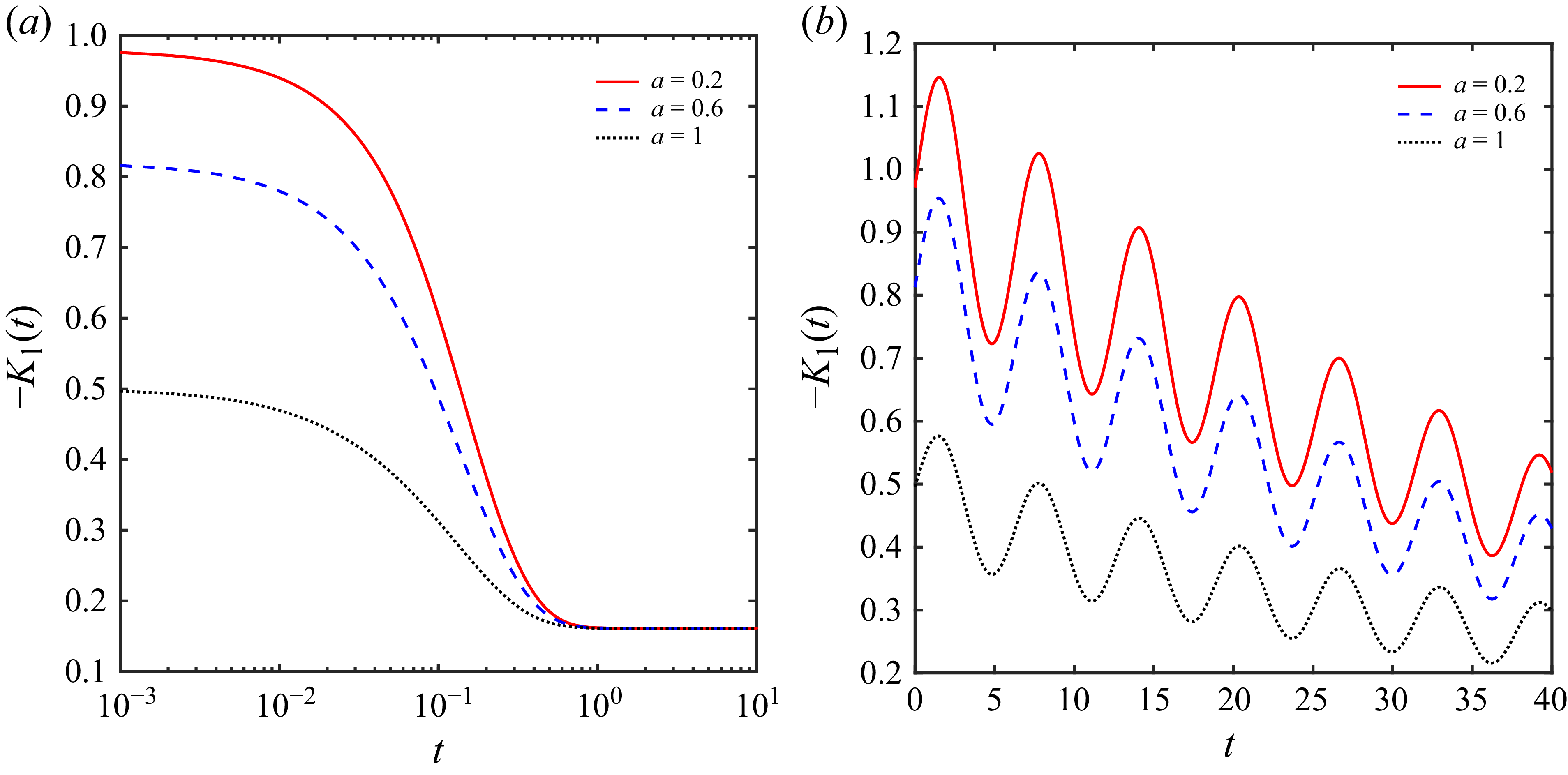
1. Introduction
Solute dispersion in a tubular two-phase system comprising a fluid core and a surrounding wall layer is relevant in diverse systems, including biological systems, chemical processing, environmental systems, microfluidics and lab-on-a-chip devices. Owing to this, Davidson & Schroter (Reference Davidson and Schroter1983), Shankar & Lenhoff (Reference Shankar and Lenhoff1991), Phillips, Kaye & Robinson (Reference Phillips, Kaye and Robinson1995), Phillips & Kaye (Reference Phillips and Kaye1998), Ng (Reference Ng2006), Ng & Rudraiah (Reference Ng and Rudraiah2008), Berg et al. (Reference Berg, Davit, Quintard and Lorthois2020), Das et al. (Reference Das, Sarifuddin, Rana and Mandal2021, Reference Das, Sarifuddin, Rana and Kumar Mandal2022) and Jiang et al. (Reference Jiang, Zeng, Fu and Wu2022) have investigated solute dispersion in a tubular two-phase system. Davidson & Schroter (Reference Davidson and Schroter1983) and Phillips et al. (Reference Phillips, Kaye and Robinson1995) analysed solute dispersion in a tubular two-phase system relevant to flow in pulmonary airways, which allowed them to consider a lower solute molecular diffusivity in the wall phase compared with the fluid phase and a small thickness of the wall phase. In the human circulatory system, the transport of solute (e.g. oxygen, nutrients and drugs) in the blood flow through the blood vessels to the surrounding tissues plays an irreplaceable role (Hunt & Bruley Reference Hunt and Bruley1978; Popel Reference Popel1981; McGuire & Secomb Reference McGuire and Secomb2001; Nicholson Reference Nicholson2001; Whiteley, Gavaghan & Hahn Reference Whiteley, Gavaghan and Hahn2002; Matzavinos et al. Reference Matzavinos, Kao, Green, Sutradhar, Miller and Friedman2009; Rana, Murthy & Gorla Reference Rana, Murthy and Gorla2017; Berg et al. Reference Berg, Davit, Quintard and Lorthois2020; Das et al. Reference Das, Sarifuddin, Rana and Mandal2021). However, blood flow is characterised by pulsatile driving force, yield stress behaviour of blood, high blood vessel thickness and substantial solute molecular diffusivity in the wall phase compared with the fluid phase. These practically important factors were not considered in the previous studies, which are explored in detail in this study.
1.1. Solute dispersion in single-phase Newtonian and non-Newtonian fluid flows
The development of solute dispersion theory originated from the classical work of Taylor (Reference Taylor1953), which provided the initial foundation for understanding the dispersion in the steady Newtonian fluid flow through a straight tube, i.e. in a single-phase shear flow. Taylor’s analysis predicted that the solute is dispersed with the combined effect of the variation of the fluid velocity across the cross-section of the tube and the molecular diffusion. Building upon Taylor’s analysis, Aris (Reference Aris1956) developed a new mathematical technique, namely the method of moments, to analyse solute dispersion in single-phase fluid flow and corrected the Taylor diffusion coefficient by incorporating the molecular diffusivity term. Taylor–Aris dispersion theory, valid for the large time limit, was further strengthened by Gill (Reference Gill1967), Gill & Sankarasubramanian (Reference Gill and Sankarasubramanian1970, Reference Gill and Sankarasubramanian1971) and Sankarasubramanian & Gill (Reference Sankarasubramanian and Gill1973) in the presence and absence of the wall absorption for a uniform and non-uniform initial distribution of the solute. They developed a new generalised dispersion model (i.e. Gill’s methodology) to capture the dispersion behaviour during the transient regime in the context of a single phase. However, this analytical technique, in the presence of wall absorption, was limited to the asymptotic regime corresponding to large times. Later, this limitation was overcome by Rana & Murthy (Reference Rana and Murthy2016a ), extending the methodology to arbitrary time scales in the presence of the wall absorption, the unsteady nature of the flow and the non-Newtonian behaviour of the fluid. To enable a systematic investigation of steady-state solute dispersion in the large time limit, Mei, Auriault & Ng (Reference Mei, Auriault and Ng1996) and Mei & Vernescu (Reference Mei and Vernescu2010) introduced an alternative analytical framework based on the method of multiple scales. Thereafter, several researchers (Chatwin Reference Chatwin1970, Reference Chatwin1975; Barton Reference Barton1983; Mazumder & Das Reference Mazumder and Das1992; Wu & Chen Reference Wu and Chen2014; Debnath et al. Reference Debnath, Jiang, Guan and Chen2022; Poddar et al. Reference Poddar, Das, Dhar and Mondal2023; Das et al. Reference Das, Mahata, Patne, Kumar and Rana2024; Huang et al. Reference Huang, Debnath, Roy, Wang, Jiang, Bég and Kuharat2024; Mahata et al. Reference Mahata, Das, Patne and Rana2025a ) adopted the above-mentioned analytical methodologies to study the solute dispersion in the steady and unsteady flows of Newtonian fluid in the context of a single phase.
Due to widespread applications in industry and biomedical engineering, the dispersion of solute in non-Newtonian fluids is getting more attention. The dispersion characteristics in non-Newtonian fluids differ significantly from those observed in Newtonian fluids, primarily due to the complex flow behaviour and rheological properties of these fluids. Lighthill (Reference Lighthill1966) discussed the applicability of the Taylor–Aris theory of dispersion to the cardiovascular system. Sharp (Reference Sharp1993) investigated the shear-augmented dispersion in steady flow of various non-Newtonian fluids (i.e. Casson, Bingham plastic and power-law fluids) in conduits based on the Taylor–Aris dispersion theory. However, these results are valid for large times exceeding approximately
 $0.5\,(a^2/D_m)$
, where
 $a$
is the radius of the pipe/height of the channel and
 $D_m$
is the molecular diffusivity of the injected solute. The pulsatile nature of fluid flow can further complicate solute dispersion in a Casson fluid, and this was investigated by Rana & Murthy (Reference Rana and Murthy2016a
) over arbitrary time scales with wall absorption in a straight tube, utilising an extended framework of Gill’s methodology. Thereafter, several researchers (Debnath et al. Reference Debnath, Saha, Mazumder and Roy2017; Rana & Murthy Reference Rana and Murthy2017b
; Roy & Bég Reference Roy and Bég2021) have investigated the effects of absorption, pulsatile flow dynamics and reactive solute transport, contributing significantly to the advancement of the understanding solute dispersion in layered fluid systems. Recent advancements in the study of solute dispersion in other non-Newtonian fluids (i.e. Herschel–Bulkley, Carreau–Yasuda, Oldroyd-B and PTT fluids) have made significant progress in unravelling the intricacies of the dispersion process (Rana & Murthy Reference Rana and Murthy2016b
,
Reference Rana and Murthyc
; Singh & Murthy Reference Singh and Murthy2023; Rana et al. Reference Rana, Das, Sarifuddin, Mandal and Patne2024; Mahata et al. Reference Mahata, Rana and Patne2025b
).
1.2. Solute dispersion in two-phase fluid–wall systems and their limitations
The exploration of solute dispersion in two-phase systems is vital owing to its broad applicability across various fields (e.g. physiological flows, chromatography, environmental flows, microfluidics and lab-on-a-chip devices), as elaborated earlier. However, the detailed understanding of solute transport mechanisms in two-phase systems, especially in the context of dispersion within microvessels and neighbouring tissue domains, remains limited despite its widespread applications. A theoretical two-phase solute transport model, applicable to gas exchange within the bronchial airways of the human lung, was proposed by Davidson & Schroter (Reference Davidson and Schroter1983). In their study (Davidson & Schroter Reference Davidson and Schroter1983), the solute dispersion in a straight tube with an absorbing wall was investigated by applying the method of the moments. The study of Davidson & Schroter (Reference Davidson and Schroter1983) was extended by Phillips et al. (Reference Phillips, Kaye and Robinson1995), investigating the effective transport coefficients, i.e. convection and dispersion coefficients, averaged over both fluid–wall phases. The asymptotic approximate solutions for the transport coefficients were derived for a thin wall layer, assuming a longer time scale for solute diffusion across the wall layer than across the fluid phase. The study of Phillips et al. (Reference Phillips, Kaye and Robinson1995) was further extended by Phillips & Kaye (Reference Phillips and Kaye1998), who analysed the time-dependent behaviour of tracer concentration at a specified downstream position after an initial pulse release, assuming the large Péclet number in their study.
Ng (Reference Ng2006) applied a homogenisation technique to explore the asymptotic behaviour of chemical species dispersion in steady and oscillatory flows within a straight tube, accounting for phase partitioning, phase exchange kinetics and absorption at the tube wall. The study of Ng (Reference Ng2006) was extended by Ng & Rudraiah (Reference Ng and Rudraiah2008) in a steady Poiseuille flow. The asymptotic transport coefficients (i.e. depletion, convection and dispersion coefficients) at long time scales were obtained by adopting the generalised dispersion model and the concentration profiles in both fluid and wall phases were determined numerically. The work of Ng & Rudraiah (Reference Ng and Rudraiah2008) was further extended by Das et al. (Reference Das, Sarifuddin, Rana and Kumar Mandal2022), who investigated unsteady solute transport in pulsatile Carreau–Yasuda fluid flow by incorporating the influence of non-Newtonian fluid rheology on the effective transport coefficients and concentration distributions in both fluid and wall phases. The solute transport in the brain microcirculation was investigated by Berg et al. (Reference Berg, Davit, Quintard and Lorthois2020) applying the asymptotic multiscale analysis for different transport regimes and the cross-section-averaged concentrations in the tube. The unsteady solute dispersion in the stenotic tube with the absorptive thin wall layer was studied numerically by Das et al. (Reference Das, Sarifuddin, Rana and Mandal2021) in the steady Casson fluid flow. Their study analysed the fraction of solute remaining in the fluid phase, the convection coefficient and the dispersion coefficient in the fluid phase with the influence of the severity of the stenosis, fluid rheology and wall absorption.
Note that the studies by Davidson & Schroter (Reference Davidson and Schroter1983), Phillips et al. (Reference Phillips, Kaye and Robinson1995) and Phillips & Kaye (Reference Phillips and Kaye1998) were limited to the steady flow of Newtonian fluid under the assumptions of a small ratio of the diffusion coefficients between the wall and fluid phases
 $(\ll 1)$
and a thin wall layer
 $(\ll 1)$
. The investigations by Ng (Reference Ng2006), Ng & Rudraiah (Reference Ng and Rudraiah2008), Jiang et al. (Reference Jiang, Zeng, Fu and Wu2022) and Das et al. (Reference Das, Sarifuddin, Rana and Kumar Mandal2022) were also limited to configurations with a thin wall layer of low diffusivity, where mass transfer across the wall was modelled using a one-dimensional diffusion framework. These analyses neglected the curvature of the wall layer and axial diffusion effects, simplifying the transport dynamics within the wall phase. However, during oxygen transport in the blood flow, the ratio of the diffusion coefficients is in the range of
 $O(10^{-1})-O(10^{0})$
(Hunt & Bruley Reference Hunt and Bruley1978; Popel Reference Popel1981; McGuire & Secomb Reference McGuire and Secomb2001; Whiteley et al. Reference Whiteley, Gavaghan and Hahn2002; Matzavinos et al. Reference Matzavinos, Kao, Green, Sutradhar, Miller and Friedman2009; Rana et al. Reference Rana, Murthy and Gorla2017; Berg et al. Reference Berg, Davit, Quintard and Lorthois2020), which is significantly higher than
 $10^{-4}$
considered in their study (Davidson & Schroter Reference Davidson and Schroter1983; Phillips et al. Reference Phillips, Kaye and Robinson1995; Phillips & Kaye Reference Phillips and Kaye1998). In general, the blood vessels are surrounded by a thick tissue layer and in the microvascular network, the thickness of the wall layer is in the range of approximately
 $O(10^{0})-O(10^{2})$
(Hunt & Bruley Reference Hunt and Bruley1978; Popel Reference Popel1981; McGuire & Secomb Reference McGuire and Secomb2001; Whiteley et al. Reference Whiteley, Gavaghan and Hahn2002; Rana et al. Reference Rana, Murthy and Gorla2017). In addition, arterial blood flow exhibits a pulsatile nature due to the periodic pumping action of the heart (Ku Reference Ku1997; Fung Reference Fung2013) and the rheological behaviour of blood is significantly influenced by its non-Newtonian characteristics in the small blood vessels (Tu & Deville Reference Tu and Deville1996; Rana & Murthy Reference Rana and Murthy2016a
). The study of Berg et al. (Reference Berg, Davit, Quintard and Lorthois2020) was limited to weak vessel–tissue coupling, treating the vascular network independently from the tissue, and focused on scenarios where solute concentrations remain negligible throughout the tissue at all times. Moreover, the numerical study of Das et al. (Reference Das, Sarifuddin, Rana and Mandal2021) overlooked analysing the effect of the pulsatile flow on the solute transport, the steady state regimes in the transportation process and mainly focused on discussing the impact of stenosis severity on the solute transport.
Motivated by these limitations, the present study aims to address several key questions: How does interphase exchange influence the dispersion as well as concentration distribution of the solute in both phases? What is the role of the unsteady flow condition and the non-Newtonian nature of the fluid on solute dispersion in the presence of interfacial transport? What are the characteristic time scales required to reach the steady state in solute dispersion for both the steady and unsteady flows? By exploring these questions, this study seeks to provide a deeper understanding of the coupled effects of flow dynamics, fluid rheology and interfacial transport on solute dispersion at arbitrary times.
2. Problem description
Consider solute transport in a long, straight, cylindrical tube surrounded by a wall (tissue) layer. This physical scenario can be modelled as two concentric cylinders having radius
 $\hat {R}_c$
and
 $\hat {R}$
(see figure 1). We assume that fluid flows only within the inner tube and transports the injected solute cloud by the combined action of advection and molecular diffusion. Following Davidson & Schroter (Reference Davidson and Schroter1983), Phillips et al. (Reference Phillips, Kaye and Robinson1995), Phillips & Kaye (Reference Phillips and Kaye1998), Nicholson (Reference Nicholson2001), Whiteley et al. (Reference Whiteley, Gavaghan and Hahn2002), Holter et al. (Reference Holter, Kehlet, Devor, Sejnowski, Dale, Omholt, Ottersen, Nagelhus, Mardal and Pettersen2017), Kutuzov, Flyvbjerg & Lauritzen (Reference Kutuzov, Flyvbjerg and Lauritzen2018), Berg et al. (Reference Berg, Davit, Quintard and Lorthois2020) and Das et al. (Reference Das, Sarifuddin, Rana and Mandal2021), we assume that within the wall region, the solute is solely transported by diffusion. Consider a one-dimensional pulsatile flow of Casson fluid in the tube. The justification for using the Casson model to describe blood rheology is outlined below.
Schematic diagram of the proposed model. A pulsatile flow of non-Newtonian Casson fluid exists in the inner tube surrounded by a wall layer mimicking a tissue layer. There is no fluid flow in the wall layer. The velocity profile shown in the figure applies to the Casson fluid subjected to a steady pressure gradient.

The Casson fluid model (Bird, Armstrong & Hassager Reference Bird, Armstrong and Hassager1977) is widely used to describe the rheology of blood, particularly in small vessels. Blood exhibits an yield stress at low shear rates due to the formation of red blood cell aggregates (rouleaux). The flow begins only when this yield stress is exceeded. The Casson model incorporates this yield-stress behaviour and agrees well with classical experimental studies on whole-blood viscosity (Cokelet Reference Cokelet1963; Merrill Reference Merrill1969; Chien Reference Chien1970). Blood also exhibits shear-thinning behaviour, where its apparent viscosity decreases as the shear rate increases. This property is captured reasonably well by the Casson relation and has been supported by several experimental investigations (Quemada Reference Quemada1978; Pries, Secomb & Gaehtgens Reference Pries, Secomb and Gaehtgens1996). In addition, this model is mathematically simple, involving only two rheological parameters (i.e. viscosity and yield stress of the fluid), compared with more complex non-Newtonian fluid models (e.g. Herschel–Bulkley, Carreau–Yasuda and viscoelastic fluid models). So, the Casson model provides an effective and physically meaningful approximation for blood in small-vessel flows, making it suitable for the present study.
In this study, it is assumed that solute exchange occurs across the fluid–wall interface, allowing the solute to penetrate the tissue layer, while the tissue layer remains impermeable to fluid to mimic the absorption of nutrients, ions, gases, etc., from the bloodstream into the tissue layer (Davidson & Schroter Reference Davidson and Schroter1983; Phillips et al. Reference Phillips, Kaye and Robinson1995; Whiteley et al. Reference Whiteley, Gavaghan and Hahn2002; Berg et al. Reference Berg, Davit, Quintard and Lorthois2020; Das et al. Reference Das, Sarifuddin, Rana and Mandal2021). An impermeable boundary encases the wall (tissue) layer. From figure 1, the domain for the fluid phase is
 $\boldsymbol{\hat {\varOmega }}_{\!{f}}=\big \{\boldsymbol{\hat {{x}}}=(\hat {r},\hat {x}):\,0\leqslant \hat {r}\leqslant \hat {R}_{c},\, -\infty \lt \hat {x}\lt \infty \big \}$
, where
 $\hat {r}$
and
 $\hat {x}$
represent the radial and axial coordinates, respectively. The wall region occupies
 $\boldsymbol{\hat {\varOmega }}_{{w}}=\big \{\boldsymbol{\hat {{x}}}=(\hat {r},\hat {x}):\,\hat {R}_{c}\leqslant \hat {r}\leqslant \hat {R},\, -\infty \lt \hat {x}\lt \infty \big \},$
where
 $\hat {R}=\hat {R}_c+\hat {\delta }_{h}$
and
 $\hat {\delta }_{h}$
is the thickness of the wall layer. Here, the ‘
 $\hat {\,}$
’ notation is used to signify a dimensional quantity.
Owing to the rheological properties of blood, the microvascular system exhibits a high concentration of red blood cells near the central axis of the vessels, while a plasma-rich, low-haematocrit (red-cell–depleted) layer forms adjacent to the vessel wall (Popel & Johnson Reference Popel and Johnson2005; Rana & Murthy Reference Rana and Murthy2017a ). The core region of blood, having concentrated red cells, can be treated as a non-Newtonian fluid, whereas the plasma-dominated peripheral layer can be considered as a Newtonian fluid. The impact of the two-phase nature of the blood on the dispersion process is significant in the microvascular system (Rana & Murthy Reference Rana and Murthy2017a ). Incorporating this blood behaviour would certainly be of interest in microvessels, but it leads to a cumbersome mathematical problem that prohibits a straightforward analytical solution. We will try to implement this in future research in this area.
2.1. Convection–diffusion equations for solute concentration
As a consequence of the above assumptions, the solute concentrations
 $\hat {C}_{\!{f}} (\hat {r},\hat {x}, \hat {t} )$
in the fluid phase and
 $\hat {C}_{{w}} (\hat {r},\hat {x}, \hat {t} )$
in the wall phase are governed by the following convective–diffusion equations:
 \begin{align} \frac {\partial \hat {C}_{\!{f}}}{\partial \hat {t}}+\hat {w}(\hat {r},\hat {t})\, \frac {\partial \hat {C}_{\!{f}}}{\partial \hat {x}}&=\hat {D}_{\!{f}}\, \frac {\partial ^{2} \hat {C}_{\!{f}}}{\partial \hat {x}^2}+\frac {\hat {D}_{\!{f}}}{\hat {r}} \frac {\partial }{\partial \hat {r}}\left (\hat {r} \frac {\partial \hat {C}_{\!{f}}}{\partial \hat {r}}\right )\!, \,\,\,\mbox{in }\, \boldsymbol{\hat {\varOmega }}_{\!{f}}\times (0,\infty ), \end{align}
 \begin{align} \mbox{and } \frac {\partial \hat {C}_{{w}}}{\partial \hat {t}}&=\hat {D}_{{w}}\, \frac {\partial ^{2} \hat {C}_{{w}}}{\partial \hat {x}^2}+\frac {\hat {D}_{{w}}}{\hat {r}} \frac {\partial }{\partial \hat {r}}\left (\hat {r} \frac {\partial \hat {C}_{{w}}}{\partial \hat {r}}\right )\!, \,\,\,\mbox{in }\, \boldsymbol{\hat {\varOmega }}_{{w}}\times (0,\infty ), \end{align}
respectively, where
 $\hat {w}(\hat {r},\hat {t})$
is the velocity of the fluid in the axial direction. The coefficients
 $\hat {D}_{\!{f}}$
and
 $\hat {D}_{{w}}$
denote the constant molecular diffusivities of the injected solute in the fluid region
 $\hat {\varOmega }_{\!{f}}$
and wall region
 $\hat {\varOmega }_{{w}}$
, respectively. The relevant initial and boundary conditions for solute concentration are as follows.
During intravascular injection, whether of a medicinal dose or a tracer used in experiments, the solute is not distributed uniformly at the moment of injection. Therefore, it is necessary to consider a non-uniform initial distribution of solute. Following Sankarasubramanian & Gill (Reference Sankarasubramanian and Gill1973), we consider that initially (
 $\hat {t}=0$
), solute is released at
 $\hat {x}=0$
, assumed to be distributed in the fluid region over the circular cross-section of radius
 $a\hat {R}_c$
 $(0\lt a\leqslant 1)$
. When
 $a=1$
, the initial distribution becomes uniform. However, there is no solute in the wall phase at
 $\hat {t}=0$
. So, the initial concentration in both phases can be represented as
 \begin{equation} \left \lbrace \!\!\begin{array}{l} \hat {C}_{\!{f}}=C_0\,\psi _1(\hat {x})\,Y_1(\hat {r}),\, \,\,\,\mbox{on }\, \boldsymbol{\hat {\varOmega }_{\!{f}}}\times \{\hat {t}=0\}, \\ \hat {C}_{{w}}=0,\, \,\,\,\mbox{on }\, \boldsymbol{\hat {\varOmega }_{{w}}}\times \{\hat {t}=0\}, \end{array}\right . \end{equation}
where the initial spreading of the solute in the fluid layer is represented by
 \begin{align} \psi _1(\hat {x})&= \frac {\hat {R}_c\,\delta (\hat {x})}{a^2}, \end{align}
 \begin{align} Y_1(\hat {r})&=\left \{ \!\!\begin{array}{ll} 1, & 0\leqslant \hat {r}\leqslant a\hat {R}_c, \,a\in (0,1],\\ 0, & a\hat {R}_c\leqslant \hat {r} \leqslant \hat {R}_c, \end{array}\right . \end{align}
 $C_{0}$
is the injected reference concentration of the solute and
 $\delta (\hat {x})$
is the Dirac delta function.
Owing to the symmetry of the concentration distribution, we have the following condition at the centreline of the tube in the fluid phase:
 \begin{align} &\frac {\partial \hat {C}_{\!{f}} }{\partial \hat {r}}=0,\,\, \mbox{ on } \{\hat {r}=0\}\times (0,\infty ). \end{align}
We assume that at the fluid–wall interface, the solute can penetrate from the fluid phase to the wall phase without any resistance. The assumption of infinite interfacial mass-transfer (also termed equilibrium partitioning or instantaneous interfacial transport) is widely used in modelling solute exchange between the fluid phase and the surrounding wall phase. Under this approximation, the solute concentration at the fluid–tissue interface is assumed to satisfy the equilibrium partition relation instantaneously, implying that the interfacial transfer kinetics are much faster than diffusion in either phase. As a result, the interfacial mass-transfer coefficient becomes effectively unbounded, and no finite kinetic resistance is introduced at the fluid–wall interface.
This approximation is justified for small and highly diffusive solutes (e.g.
 $\rm O_2$
,
 $\rm CO_2$
, etc.) whose endothelial crossing time is negligible compared with intravascular or tissue diffusion times (Popel Reference Popel1981; Sharan, Aminataei & Singh Reference Sharan, Aminataei and Singh1987; Kellen Reference Kellen2002; Whiteley et al. Reference Whiteley, Gavaghan and Hahn2002; Popel & Johnson Reference Popel and Johnson2005). The microvascular endothelium, especially in continuous and fenestrated vessels, exhibits high permeability for such solutes, resulting in minimal kinetic resistance at the interface (Michel & Curry Reference Michel and Curry1999; Fung Reference Fung2013). Hence, for small solutes and highly permeable microvessels, assuming infinite interfacial transport is physiologically reasonable and widely adopted in theoretical formulations.
However, in some other physiological situations, the endothelial interface provides a finite resistance to solute exchange, so interfacial transport cannot be described by instantaneous equilibrium (Friedland Reference Friedland1978; Matzavinos et al. Reference Matzavinos, Kao, Green, Sutradhar, Miller and Friedman2009; Rana et al. Reference Rana, Murthy and Gorla2017; Berg et al. Reference Berg, Davit, Quintard and Lorthois2020). In this case, the solute flux is controlled by a finite interfacial mass-transfer coefficient, which produces a measurable concentration difference across the interface. Such conditions arise for macromolecules (including peptides, proteins and lipoproteins) (Michel & Curry Reference Michel and Curry1999), and during transport across tight endothelial barriers such as the blood–brain barrier (Berg et al. Reference Berg, Davit, Quintard and Lorthois2020), and retinal capillaries (Friedland Reference Friedland1978). In these situations, the interface plays an important role in limiting overall transport. Therefore, considering the resistance at the interface would be interesting, but it leads to a mathematically cumbersome problem. Thus, we have not considered resistance at the interface in the present study.
Following Davidson & Schroter (Reference Davidson and Schroter1983), Phillips et al. (Reference Phillips, Kaye and Robinson1995), Whiteley et al. (Reference Whiteley, Gavaghan and Hahn2002) and Das et al. (Reference Das, Sarifuddin, Rana and Mandal2021) and considering the continuity of the concentration flux at the fluid–wall interface, the relevant boundary conditions are given by
 \begin{align} &\hat {C}_{{w}}=\beta _{{p}} \,\hat {C}_{\!{f}}, \,\, \hat {D}_{\!{f}}\,\frac {\partial \hat {C}_{\!{f}} }{\partial \hat {r}}=\hat {D}_{{w}}\,\frac {\partial \hat {C}_{{w}} }{\partial \hat {r}},\,\, \mbox{ on } \left\{\hat {r}=\hat {R}_c\right\}\times (0,\infty ), \end{align}
where
 $\beta _{{p}}$
is the ratio of the solute concentration in the wall phase to the concentration in the fluid phase at equilibrium, i.e. partitioning coefficient at the fluid–wall interface. We assume that the outer boundary of the wall layer acts as an impermeable layer, meaning that no solute can penetrate through this boundary. Mathematically, this can be expressed as
 \begin{align} &\frac {\partial \hat {C}_{{w}} }{\partial \hat {r}}=0,\,\, \mbox{ on } \{\hat {r}=\hat {R}\}\times (0,\infty ). \end{align}
Since the amount of the solute is finite in the system, the solute vanishes far from the injection location, and we have the following conditions:
 \begin{align} \hat {C}_{\!{f}}&=0,\,\frac {\partial \hat {C}_{\!{f}}}{\partial \hat {x}}=0,\,\, \mbox{ as } \hat {x}\rightarrow \pm \infty ,\,\,\hat {t}\in (0,\infty ), \end{align}
 \begin{align} \mbox{and } \hat {C}_{{w}}&=0,\,\frac {\partial \hat {C}_{{w}}}{\partial \hat {x}}=0,\,\, \mbox{ as } \hat {x}\rightarrow \pm \infty ,\,\,\hat {t}\in (0,\infty ). \end{align}
2.2. Non-dimensionalisation
The following scaled variables are utilised to obtain the non-dimensional form of the above governing equations and velocity profile:
 \begin{align} &\displaystyle x=\frac {\hat {x} \hat {D}_{\!{f}}}{W_0 \hat {R}_c^2}, \quad r=\frac {\hat {r}}{\hat {R}_c},\quad R=\frac {\hat {R}}{\hat {R}_c}, \quad t=\hat {\omega }\hat {t},\quad w=\frac {\hat {w}}{W_0}, \quad C_{\!{f}} =\frac {\hat {C}_{\!{f}}}{C_0},\quad C_{{w}} =\frac {\hat {C}_{{w}}}{C_0}, \nonumber \\ &\tau =\frac {\hat {\tau }}{\hat {\mu }\left (W_0/\hat {R}_c\right )}, \quad \tau _{{y}}=\frac {\hat {\tau }_{{y}}}{\hat {\mu }\left (W_0/\hat {R}_c\right )}, \end{align}
where
 $W_0$
is the characteristic velocity defined by
 $(P_0\hat {R}_c^2)/(4\hat {\mu })$
,
 $\hat {\tau }$
is the shear stress,
 $\hat {\tau }_{{y}}$
is the yield stress,
 $\hat {\omega }=2\,\pi \,f$
is the frequency of the pressure pulsation and
 $f$
denotes the pulse frequency. In the blood flow, the frequency
 $f$
ranges from
 $50{-}100$
beats per minute, and it is considered as
 $1.2\, \rm Hz$
at the normal heart rate of 72 beats per minute (Rana et al. Reference Rana, Das, Sarifuddin, Mandal and Patne2024). This oscillation in the pressure gradient leads to an oscillating flow field having the same frequency.
With these scaled variables, the domains of the considered problem reduce to
 $\boldsymbol{\varOmega }_{\!{f}}=\big \{\boldsymbol{{x}}:\,0\leqslant r\leqslant 1,\, -\infty \lt x \lt \infty \big \}$
and
 $\boldsymbol{\varOmega }_{{w}}=\big \{\boldsymbol{{x}}:\,1\leqslant r \leqslant R,\, -\infty \lt x \lt \infty \big \}$
. The convection–diffusion equations transform to
 \begin{align} P^2_{\omega }\ \frac {\partial C_{\!{f}}}{\partial t}+w \,\frac {\partial C_{\!{f}}}{\partial x}&=\frac {1}{{\boldsymbol{Pe^2}}} \frac {\partial ^{2} C_{\!{f}}}{\partial x^2}+\frac {1}{r} \frac {\partial }{\partial r}\left (r \frac {\partial C_{\!{f}}}{\partial r}\right )\!, \,\,\,\mbox{in }\, \boldsymbol{\varOmega }_{\!{f}}\times (0,\infty ); \end{align}
 \begin{align} P^2_{\omega }\ \frac {\partial C_{{w}}}{\partial t}&=\frac {\lambda }{{\boldsymbol{Pe^2}}} \frac {\partial ^{2} C_{{w}}}{\partial x^2}+\frac {\lambda }{r} \frac {\partial }{\partial r}\left (r \frac {\partial C_{{w}}}{\partial r}\right )\!, \,\,\,\mbox{in }\, \boldsymbol{\varOmega }_{{w}}\times (0,\infty ), \end{align}
with the following dimensionless form of initial and boundary conditions:
 \begin{align} &\qquad\quad C_{\!{f}}=\,\psi (x)\,Y(r),\, \,\,\,\mbox{on }\, \boldsymbol{\varOmega _{\!{f}}}\times \{t=0\} \nonumber \\ &\qquad\qquad \mbox{ and } \hspace {.1cm} C_{{w}}=0,\, \,\,\,\mbox{on }\, \boldsymbol{\varOmega }_{{w}}\times \{t=0\}, \end{align}
 \begin{align} &\qquad\qquad \frac {\partial C_{\!{f}} }{\partial r}=0, \,\, \mbox{ on } \{r=0\}\times (0,\infty ), \end{align}
 \begin{align} & \beta _{{p}} C_{\!{f}}= C_{{w}}, \quad \frac {\partial C_{\!{f}} }{\partial r}=\lambda \,\frac {\partial C_{{w}} }{\partial r},\,\, \mbox{ on } \{r=1\}\times (0,\infty ), \end{align}
 \begin{align} &\qquad\quad \frac {\partial C_{{w}} }{\partial r}=0, \,\, \mbox{ on } \{r=R\}\times (0,\infty ), \end{align}
 \begin{align} &\quad C_{\!{f}}= 0,\,\frac {\partial C_{\!{f}}}{\partial x}= 0,\,\, \mbox{ as } x\rightarrow \pm \infty ,\,\,t\in (0,\infty ), \end{align}
 \begin{align} &\,\, \mbox{and } C_{{w}}= 0,\,\frac {\partial C_{{w}}}{\partial x}= 0,\,\, \mbox{ as } x\rightarrow \pm \infty ,\,\,t\in (0,\infty ). \end{align}
Here, the non-dimensional form of the initial condition is
 \begin{align} \psi (x)&= \frac {\delta (x)}{a^2\,{\textit{Pe}}}, \end{align}
 \begin{align} Y(r)&=\left \{\!\! \begin{array}{ll} 1, & 0\leqslant r\leqslant a,\\ 0, & a\leqslant r \leqslant 1, \end{array}\right . \end{align}
 $\lambda = \hat {D}_{{w}}/\hat {D}_{\!{f}}$
represents the ratio of the diffusion coefficient within the wall phase
 $\varOmega _{{w}}$
to that of the fluid phase
 $\varOmega _{\!{f}}$
,
 ${\boldsymbol{Pe}}= W_0 \hat {R}_c/\hat {D}_{\!{f}}$
is Péclet number, which is the ratio of diffusive time scale
 $(\hat {R_{c}}^2/\hat {D}_{f})$
to convective time scale
 $(\hat {R_{c}}/W_0)$
. When
 ${\textit{Pe}}\gg 1$
, it implies that
 $\hat {R_{c}}^2/\hat {D}_{f}\gg \hat {R_{c}}/W_0$
, i.e. the characteristic time for diffusion across the cross-section of the tube is higher than the characteristic time for convection, signifying that the convective transport is dominant. The opposite scenario occurs when
 ${\textit{Pe}} \ll 1$
.
Here
 $R=1+\delta _{h}$
,
 $\delta _{h} =\hat {\delta }_{h}/ \hat {R}_c$
is the dimensionless thickness of the wall layer and
 $P^2_{\omega }=\hat {\omega } \hat {R_{c}}^2/\hat {D}_{\!{f}}= \alpha ^2\ \rm Sc$
is the oscillatory Péclet number which is associated with the Womersley frequency parameter
 $\alpha = \hat {R_{c}}\sqrt {\hat {\omega } / (\hat {\mu }/\hat {\rho } )}$
and the Schmidt number (Sc
 $=\hat {\mu }/\hat {\rho }\hat {D}_{\!{f}})$
. The time scale of the dispersion is influenced by the parameter
 $P^2_{\omega }$
, which occurs in the study owing to the pulsatile nature of the flow and is the ratio of the characteristic time for diffusion
 $(\hat {R_{c}}^2/\hat {D}_{f})$
to the period of the oscillation
 $(1/\hat {\omega })$
. In this study, we have mainly discussed the effect of four parameters
 $\lambda$
,
 $\beta _{p}$
,
 $\delta _{h}$
and
 $a$
on the dispersion of the solute, considering the pulsatile fluid flow.
By following Rana & Murthy (Reference Rana and Murthy2016a
), the velocity profiles
 $w^{in}_{p}(t)$
for the plug flow
 $(0 \leqslant r \leqslant r_p(t))$
and
 $w^{out}_{p}(t,r)$
outside the plug flow
 $(r_p(t) \leqslant r \leqslant 1)$
regions are derived as
 \begin{align} w^{in}_{p}(t)&= \frac {p(t)}{2}\left [1-\frac {8}{3} r_p^{1 / 2}+2 r_p-\frac {1}{3} r_p^2\right ] \nonumber \\ & \quad -\varepsilon \frac {p^{\prime }(t)}{32}\left [3-\frac {1144}{147} r_p^{1 / 2}\!+\frac {320}{63} r_p+\frac {4}{3} r_p^2-\frac {16}{9} r_p^{5 / 2}\!+\frac {65}{441} r_p^4\right ]\!, 0 \leqslant r \leqslant r_p(t), \end{align}
 \begin{align} w^{out}_{p}(t,r)&=\frac {p(t)}{2}\left [\left (1-r^2\right )-\frac {8}{3} r_p^{1 / 2}\left (1-r^{3 / 2}\right )+2 r_p(1-r)\right ] \nonumber \\ &\quad -\varepsilon \frac {p^{\prime }(t)}{2}\left [\frac {3}{16}-\frac {r^2}{16}\left (4-r^2\right )-\frac {r_p^{1 / 2}}{16}\left (\frac {1144}{147}-\frac {16}{3}\left (r^2+r^{3 / 2}\right )+\frac {424}{147} r^{7 / 2}\right )\!\right ] \nonumber \\ &\quad -\varepsilon p^{\prime }(t) \frac {r_p}{32}\left [\frac {320}{63}+\frac {128}{63} r^3-\frac {64}{9} r^{3 / 2}\right ]\!,\, r_p(t) \leqslant r \leqslant 1, \end{align}
respectively, where
 $\varepsilon =\alpha ^2$
is chosen as a perturbation parameter since we have considered the small-sized tube in which the non-Newtonian nature of the fluid is predominant and the value of
 $\alpha$
is small
 $(\ll 1)$
,
 $r_p(t)$
is the dimensionless radius of the plug flow region,
 $p^{\prime }(t)=\mathrm{d} p / \mathrm{d} t$
,
 $p(t)=2 (1+e \sin (t ) )$
is the pulsatile pressure gradient combined with steady and unsteady components and
 $e$
is the amplitude of the fluctuating pressure component. Note that in the pulsatile flow,
 $r_p(t)$
changes during the cycle of oscillation in the presence of the yield stress parameter
 $\tau _{y}$
and the applied pressure gradient, and it is obtained as
 \begin{align} r_p(t)=R_{p}-\varepsilon \frac {p^{\prime }(t)}{p(t)}\Bigg [\frac {R_{p}}{4}-\frac {2}{3}R_{p}^{3/2}+\frac {R_{p}^2}{2}-\frac {R^3_{p}}{12}\Bigg ], \end{align}
where
 $R_{p}(t)=\tau _{y}/p(t).$
For steady flow,
 $R_{p}$
takes the constant value
 $\tau _{y}/2$
for fixed
 $\tau _{y}$
.
The corresponding solution for a pulsatile Newtonian fluid flow can be obtained from the above solution (2.6), considering
 $\tau _{y}=0$
. Alternatively, by applying the Laplace transformation, the velocity profile for Newtonian fluid in the pulsatile flow is obtained as (Sud & Sekhon Reference Sud and Sekhon1985; Das et al. Reference Das, Mahata, Patne, Kumar and Rana2024)
 \begin{align} w(r,t)=& \,w_0(r)-\frac {4\,e}{\alpha ^2}\cos {t}+\frac {2\,e}{\alpha ^2}\,\frac {J_0(\sqrt {-i\,\alpha ^2}r)}{J_0(\sqrt {-i\,\alpha ^2})}\,\exp {(it)}+\frac {2\,e}{\alpha ^2}\,\frac {J_0(\sqrt {i\,\alpha ^2}r)}{J_0(\sqrt {i\,\alpha ^2})}\,\exp {(-it)}\nonumber \\ & +8\,e\,\sum _{n=1}^{\infty } \frac {\alpha ^2 \,J_0(\xi _{n}r)}{\left (\xi _{n}^5+\alpha ^4\,\xi _{n}\right )\,J_1(\xi _{n})}\,\exp {\left (-\frac {\xi _{n}^2}{\alpha ^2}\,t\right )}, \end{align}
where
 $w_0(r)=(1-r^2)$
is the velocity profile for the steady flow,
 $J_0$
and
 $J_1$
are the Bessel functions of the first kind of order zero and order one, respectively, and
 $\xi _{n}$
are the roots of the following transcendental equation:
 \begin{align} J_0(\xi _{n})=0,\,\,\, n=1,2,3,\ldots \,. \end{align}
The fluid velocity strongly depends on
 $e$
and
 $\alpha$
, which affects the solute dispersion in the pulsatile flow. For the steady flow situation,
 $w(r,t)=w_0(r)$
owing to vanishing contribution from the time-dependent terms in the above solution.
3. Method of solution for solute concentration
The obtained velocity profile is plugged into the convective–diffusive equation (2.4a ). The solute concentration in the fluid and wall phases is obtained by solving the resulting (2.4a ) and (2.4b ). The series solution method (Gill’s methodology) adopted by Gill & Sankarasubramanian (Reference Gill and Sankarasubramanian1970) and Sankarasubramanian & Gill (Reference Sankarasubramanian and Gill1973) was primarily focused on the fluid phase only, and the solution procedure described in their study was applicable solely to this particular phase. However, in this study, we have extended and generalised Gill’s methodology with rigorous mathematical derivations and obtained the time-dependent solution for solute concentration over two phases, i.e. fluid and wall phases.
To analyse solute dispersion, we express the solute concentrations
 $C_{\!{f}}(t, x, r)$
and
 $C_{{w}}(t, x, r)$
in the fluid phase
 $\varOmega _{\!{f}}$
and wall phase
 $\varOmega _{{w}}$
, respectively, as an infinite series
 \begin{equation} C_{\!{f}}(t, x, r)=\sum _{i=0}^{\infty } f_i(t, r) \frac {\partial ^i \overline {C}}{\partial x^i}, \end{equation}
and
 \begin{equation} C_{{w}}(t, x, r)=\sum _{i=0}^{\infty } g_i(t, r) \frac {\partial ^i \overline {C}}{\partial x^i}. \end{equation}
The mean concentration
 $\overline {C}(t, x)$
is defined by
 \begin{equation} \overline {C}(t, x)=\frac {2}{R^2}\left [\int _{0}^1 r \,C_{\!{f}}\, {\rm d} r+\int _{1}^{R} r\, C_{{w}} \,{\rm d} r\right ]\!, \end{equation}
where
 $R=1+\delta _{h}$
. Multiplying by
 $r$
and integrating with respect to
 $r$
from 0 to 1, (2.4a
) is transformed to
 \begin{align} P^2_{\omega } \,\frac {\partial }{\partial t}\left (\int _{0}^{1} r\,C_{\!{f}} \,\mathrm{d} r\right ) + \frac {\partial }{\partial x}\left (\int _{0}^{1} r\,w\,C_{\!{f}} \,\mathrm{d} r\right )=\frac {\partial C_{\!{f}}}{\partial r}(t,x,1)+\frac {1}{{\textit{Pe}}^2}\, \frac {\partial ^2}{\partial x^2}\left (\int _{0}^{1} r\,C_{\!{f}} \,\mathrm{d} r\right )\!. \end{align}
Similarly, by multiplying by
 $r$
and integrating with respect to
 $r$
from 1 to R, (2.4b
) is reduced to
 \begin{align} P^2_{\omega } \,\frac {\partial }{\partial t}\left (\int _{1}^{R} r\,C_{{w}} \,\mathrm{d} r\right )=-\lambda \,\frac {\partial C_{{w}}}{\partial r}(t,x,1)+\frac {\lambda }{{\textit{Pe}}^2}\, \frac {\partial ^2}{\partial x^2}\left (\int _{1}^{R} r\,C_{{w}} \,\mathrm{d} r\right )\!. \end{align}
Now adding (3.3) and (3.4), and multiplying the resulting equation by
 $2/R^2$
, we have
 \begin{align} P^2_{\omega } \,\frac {\partial \overline {C}}{\partial t} =\frac {\lambda }{{\textit{Pe}}^2}\, \frac {\partial ^2 \overline {C}}{\partial x^2}+\frac {2}{R^2}\frac {\left (1-\lambda \right )}{{\textit{Pe}}^2}\,\frac {\partial ^2}{\partial x^2}\left (\int _{0}^{1} r\,C_{\!{f}} \,\mathrm{d} r\right )-\frac {2}{R^2}\,\frac {\partial }{\partial x}\left (\int _{0}^{1} r\,w\,C_{\!{f}} \,\mathrm{d} r\right )\!. \end{align}
We substitute the expression of
 $C_{\!{f}}$
defined in (3.1a
) into (3.5) and the dispersion model for
 $\overline {C}$
is as follows:
 \begin{equation} P^2_{\omega } \,\frac {\partial \overline {C}}{\partial t}=\sum _{i=1}^{\infty } K_i(t) \frac {\partial ^i \overline {C}}{\partial x^i}, \end{equation}
where the transport coefficients
 $K_{i}(t)$
are obtained by
 \begin{eqnarray} K_{i}(t)=\delta _{i2}\,\frac {\lambda }{{\textit{Pe}}^2}+\frac {2}{R^2}\frac {\left (1-\lambda \right )}{{\textit{Pe}}^2}\,\int _{0}^{1}r\,f_{i-2}(t,r)\,\mathrm{d} r-\frac {2}{R^2}\int _{0}^{1}r\,w(t,r)\,f_{i-1}(t,r) \,\mathrm{d} r, \nonumber \\i=1,2\ldots , \end{eqnarray}
and
 $\delta _{ij}$
denotes Kronecker delta
 \begin{equation} \delta _{ij} = \left \{\!\! \begin{array}{ll} 1, & i=j,\\[2pt] 0, & i\neq j. \end{array} \right . \end{equation}
Here,
 $K_1$
and
 $K_2$
are the convection and dispersion coefficients, respectively, and
 $K_i(t)\,(i\geqslant 3)$
are the higher-order transport coefficients. Note that, owing to this practical necessity, we have not imposed restrictions on
 $\lambda$
and
 $\delta _{h}$
values in the present study while deriving expressions for the transport coefficients.
Upon substituting (3.1) and (3.6) into (2.4), and equating the coefficients of
 $\partial ^k \overline {C}/\partial x^k$
, we obtain the following system of partial differential equations:
 \begin{align} P^2_{\omega }\ \frac {\partial f_k}{\partial t}=&\frac {1}{r} \frac {\partial }{\partial r} \left (r\frac {\partial f_k}{\partial r}\right ) -\left (w+K_1\right ) f_{k-1}+\left (\frac {1}{{\boldsymbol{Pe^2}}}- K_2\right ) f_{k-2}\nonumber \\ &\,-\chi _{k}\sum \limits _{j=3}^{k}K_{j}\left (t\right )f_{k-j}, \quad k=0,1,2,\ldots \end{align}
and
 \begin{align} P^2_{\omega }\ \frac {\partial g_k}{\partial t}=&\frac {\lambda }{r} \frac {\partial }{\partial r} \left (r\frac {\partial g_k}{\partial r}\right ) -K_1 \,g_{k-1}+\left (\frac {\lambda }{{\boldsymbol{Pe^2}}}- K_2\right ) g_{k-2}\nonumber \\ &\,-\chi _{k}\sum \limits _{j=3}^{k}K_{j}\left (t\right )g_{k-j}, \quad k=0,1,2,\ldots \end{align}
where
 $f_{-1}=f_{-2}=g_{-1}=g_{-2}=0$
, and
 \begin{equation} \chi _{k} = \left \{ \begin{array}{ll} 1, & k\geqslant 3,\\[2pt] 0, & k\lt 3. \end{array} \right . \end{equation}
The initial conditions are given by
 \begin{align} f_{k}(0,r)&=\frac {R^2\,Y(r)}{2\int _0^1 r\,Y(r)\ \mathrm{d} r}\,\delta _{k0}, \end{align}
 \begin{align} \mbox{and}\quad g_{k}(0,r)&=0,\,\,k=0,1,2,\ldots , \end{align}
and the boundary conditions are as follows:
 \begin{align} \frac {\partial f_{k}}{\partial r}\left (t,0\right )&=0, \end{align}
 \begin{align} \beta _{p}\,f_{k}(t,1)&=g_{k}(t,1)\!, \end{align}
 \begin{align} \frac {\partial f_{k}}{\partial r}(t,1)&=\lambda \,\frac {\partial g_{k}}{\partial r}(t,1)\!, \end{align}
 \begin{align} \frac {\partial g_{k}}{\partial r}\left (t,R\right )&=0,\,\,k=0,1,2,\ldots , \end{align}
with an additional condition obtained from (3.1) and (3.2)
 \begin{eqnarray} \int _0^1 r \,f_{k}\,\left (t,r\right ){\rm d} r+\int _1^R r \,g_{k}\,\left (t,r\right ){\rm d} r=\frac {R^2}{2}\delta _{k0}, \end{eqnarray}
where
 $\delta _{ij}$
denotes Kronecker delta. The additional condition (3.11g
) has been explicitly used to find the steady state solutions for
 $f_k(t,r)$
and
 $g_k(t,r)$
 $(k=0,1,2,\ldots )$
as
 $t\rightarrow \infty$
. Moreover, the time-dependent solutions for
 $f_k(t,r)$
and
 $g_k(t,r)$
 $(k=0,1,2,\ldots )$
must also satisfy this condition. The initial and boundary conditions for the mean concentration
 $\overline {C}(t, x)$
are given by
 \begin{align} \overline {C}(0, x)&=\frac {\delta (x)}{R^2\,{\textit{Pe}}}, \end{align}
 \begin{align} \mbox{and } \overline {C}(t, \pm \infty )&=\frac {\partial \overline {C}}{\partial x}(t, \pm \infty )=0, \end{align}
respectively.
Now our aim is to determine the transport coefficients
 $K_{i}(t)$
by solving (3.9a
) and (3.9b
) with the relevant conditions (3.11). By solving (3.9a
) and (3.9b
) for
 $k = 0$
, the solutions for
 $f_0(t,r)$
and
 $g_0(t,r)$
are obtained as
 \begin{equation} f_{0}(r,t) = \frac {R^2}{1+\beta _{{p}}\left (R^2-1\right )}+\sum _{n=0}^\infty \frac {R^2 J_1(\mu _n\,\textit{a})}{a\,\mu _n \,I_n}\, J_0(\mu _n r)\,\mathrm{e}^{-(\mu _n/P_\omega )^2 t} \end{equation}
and
 \begin{equation} g_{0}(r,t) = \frac {R^2\beta _{{p}}}{1+\beta _{{p}}\!\left (R^2-1\right )}+\sum _{n=0}^\infty \frac {R^2 J_1(\mu _n\,\textit{a})}{a\,\mu _n \,I_n}\left [\! P_nJ_0 \left (\!\frac {\mu _n r}{\sqrt {\lambda }}\!\right ) + Q_nY_0 \left (\!\frac {\mu _n r}{\sqrt {\lambda }}\!\right )\!\right ]\mathrm{e}^{-(\mu _n/P_\omega )^2 t}, \end{equation}
respectively, where
 $J_i$
and
 $Y_i$
are the Bessel functions of the first kind and second kind, respectively, with order
 $i$
. Here,
 \begin{align} \displaystyle P_n &= \frac {\beta _{{p}}\,J_0(\mu _n)\,Y_1\left (\dfrac {\mu _n R}{\sqrt {\lambda }}\right )}{\left [J_0\left (\dfrac {\mu _n}{\sqrt {\lambda }}\right )Y_1\left (\dfrac {\mu _n R}{\sqrt {\lambda }}\right )-J_1\left (\dfrac {\mu _n R}{\sqrt {\lambda }}\right )Y_0\left (\dfrac {\mu _n }{\sqrt {\lambda }}\right )\right ]}, \end{align}
 \begin{align} \displaystyle Q_n &= -\frac {\beta _{{p}}\,J_0(\mu _n)\,J_1\left (\dfrac {\mu _n R}{\sqrt {\lambda }}\right )}{\left [J_0\left (\dfrac {\mu _n}{\sqrt {\lambda }}\right )Y_1\left (\dfrac {\mu _n R}{\sqrt {\lambda }}\right )-J_1\left (\dfrac {\mu _n R}{\sqrt {\lambda }}\right )Y_0\left (\dfrac {\mu _n }{\sqrt {\lambda }}\right )\right ]}, \end{align}
 $\mu _n$
are the roots of the following transcendental equation:
 \begin{align} & \displaystyle J_1(\mu _n)\left [J_0\left (\frac {\mu _n }{\sqrt {\lambda }}\right )Y_1\left (\frac {\mu _n R}{\sqrt {\lambda }}\right )-J_1\left (\frac {\mu _n R}{\sqrt {\lambda }}\right )Y_0\left (\frac {\mu _n }{\sqrt {\lambda }}\right )\right ] \nonumber \\ &\,\,\,\,=\beta _p \,\sqrt {\lambda }\,J_0(\mu _n)\left [J_1\left (\frac {\mu _n }{\sqrt {\lambda }}\right )Y_1\left (\frac {\mu _n R}{\sqrt {\lambda }}\right )-J_1\left (\frac {\mu _n R}{\sqrt {\lambda }}\right )Y_1\left (\frac {\mu _n }{\sqrt {\lambda }}\right )\right ]\!, \,\, n=0,1,2,\ldots , \end{align}
and the orthogonality relation for the eigenfunctions is presented in Appendix B, and it provides
 \begin{equation} \displaystyle I_n=\int _{0}^{1} r \,J_0^2(\mu _n r) \,\mathrm{d} r + \frac {1}{\beta _{{p}}}\int _{1}^{R} r \,\left [P_n\,J_0 \left (\frac {\mu _n r}{\sqrt {\lambda }}\right ) + Q_n\,Y_0 \left (\frac {\mu _n r}{\sqrt {\lambda }}\right )\right ]^2 \,\mathrm{d} r. \end{equation}
By using the solution for
 $f_0(t,r)$
, the convection coefficient
 $K_1$
is obtained from (3.7),
 \begin{align} \displaystyle K_{1}(t)&=-\frac {2}{R^2}\int _{0}^{1}r\,w(t,r)\,f_{0}(t,r) \,\mathrm{d} r\nonumber \\ &=-\frac {\overline {w}(t)}{1+\beta _{{p}}\left (R^2-1\right )}-\frac {2}{R^2}\sum _{n=0}^\infty \frac {R^2 J_1(\mu _n\,\textit{a})}{a\,\mu _n \,I_n}\, B_{n}(t)\,\mathrm{e}^{-(\mu _n/P_\omega )^2 t}, \end{align}
where
 $\overline {w}(t)$
is the average velocity of the fluid, and it is given by
 \begin{align} \displaystyle \overline {w}(t)&=2\,\int _{0}^{1}r\,w(t,r) \,\mathrm{d} r, \end{align}
 \begin{align} \mbox{and }\displaystyle B_{n}(t)&=\int _{0}^{1}r\,w(t,r)\,J_0(\mu _n r)\,\mathrm{d} r. \end{align}
The coefficient
 $B_{n}(t)$
is obtained numerically. From (3.19), the solute convection strongly depends on the partitioning coefficient of the concentrations at the fluid–wall interface, the ratio of the diffusion coefficients within the wall phase to the fluid phase, the thickness of the wall layer and the flow pulsatility.
By using the eigenfunction expansion method, (3.9a
) and (3.9b
) for
 $k = 1$
are solved and the solution for
 $f_1(t,r)$
and
 $g_1(t,r)$
are obtained as
 \begin{align} f_{1}(r,t)&=- \frac {R^2}{P_\omega ^2\Big (\! 1+\left (R^2-1\right )\beta _{{p}}\!\Big )}\sum _{n=0}^\infty \frac {1}{I_n} \left \lbrace \int _0^t \!\Big (B_n(s)+D_n \, K_1(s)\!\Big )\mathrm{e}^{(\mu _n/P_\omega )^2 s} \mathrm{d}s\right \rbrace J_0(\mu _n r) \nonumber \\ &\times \mathrm{e}^{-(\mu _n/P_\omega )^2 t}-\frac {1}{P_\omega ^2}\sum _{n=0}^\infty \sum _{m=0}^\infty \frac {R^2 J_1(\mu _m\,\textit{a})}{a\,\mu _m\, I_m\,I_n} \left \lbrace \int _0^t B^{*}_{mn}(s)\,\mathrm{e}^{(\mu _n^2-\mu _m^2)s/P_\omega ^2} \mathrm{d}s\right \rbrace J_0(\mu _n r)\nonumber \\ &\times \mathrm{e}^{-(\mu _n/P_\omega )^2 t}-\frac {1}{P_\omega ^2}\sum _{n=0}^\infty \frac {R^2 J_1(\mu _n\,\textit{a})}{a\,\mu _n \,I_n} \left \lbrace \int _0^t K_1(s)\mathrm{d}s\right \rbrace J_0(\mu _n r)\,\mathrm{e}^{-(\mu _n/P_\omega )^2 t}, \end{align}
and
 \begin{align} &g_{1}(r,t)\nonumber \\ &=- \frac {R^2}{P_\omega ^2\Big (\! 1+\left (R^2-1\right )\beta _{{p}}\!\Big )}\sum _{n=0}^\infty \frac {1}{I_n} \left \lbrace \int _0^t \Big (B_n(s)+D_n \, K_1(s)\Big )\mathrm{e}^{(\mu _n/P_\omega )^2 s} \mathrm{d}s\right \rbrace \bigg [P_nJ_0 \left (\!\frac {\mu _n r}{\sqrt {\lambda }}\!\right ) \nonumber \\ &\quad + Q_nY_0 \left (\!\frac {\mu _n r}{\sqrt {\lambda }}\!\right )\!\bigg ]\,\mathrm{e}^{-(\mu _n/P_\omega )^2 t}-\frac {1}{P_\omega ^2}\sum _{n=0}^\infty \sum _{m=0}^\infty \frac {R^2 J_1(\mu _m\,\textit{a})}{a\,\mu _m\, I_m\,I_n} \left \lbrace \int _0^t \!B^{*}_{mn}(s)\,\mathrm{e}^{(\mu _n^2-\mu _m^2)s/P_\omega ^2} \mathrm{d}s\right \rbrace \nonumber \\ &\quad\times \bigg [P_nJ_0 \left (\frac {\mu _n r}{\sqrt {\lambda }}\right ) + Q_nY_0 \left (\frac {\mu _n r}{\sqrt {\lambda }}\right )\bigg ]\,\mathrm{e}^{-(\mu _n/P_\omega )^2 t}-\frac {1}{P_\omega ^2}\sum _{n=0}^\infty \frac {R^2 J_1(\mu _n\,\textit{a})}{a\,\mu _n\, I_n} \left \lbrace \int _0^t K_1(s)\mathrm{d}s\right \rbrace \nonumber \\ &\quad\times \bigg [P_nJ_0 \left (\frac {\mu _n r}{\sqrt {\lambda }}\right ) + Q_nY_0 \left (\frac {\mu _n r}{\sqrt {\lambda }}\right )\bigg ]\,\mathrm{e}^{-(\mu _n/P_\omega )^2 t}, \end{align}
respectively, where
 \begin{equation} \displaystyle B^{*}_{mn}(s) = \int _{0}^{1}r\,w(s,r)\,J_0(\mu _n r)\,J_0(\mu _m r)\,\mathrm{d} r, \end{equation}
and
 \begin{equation} \displaystyle D_n = \frac {J_1(\mu _n)}{\mu _n }+\frac {P_n\left [R\,J_1 \left (\dfrac {\mu _n R}{\sqrt {\lambda }}\right )-J_1\left (\dfrac {\mu _n }{\sqrt {\lambda }}\right )\right ]+Q_n\left [R\,Y_1 \left (\dfrac {\mu _n R}{\sqrt {\lambda }}\right )-Y_1\left (\dfrac {\mu _n }{\sqrt {\lambda }}\right )\right ]}{\dfrac {\mu _n }{\sqrt {\lambda }}}. \end{equation}
The coefficient
 $B^{*}_{mn}(s)$
is obtained numerically. Note that the dispersion coefficient
 $K_2$
represents solute dispersion due to shear-enhanced dispersion and molecular diffusion. Now, the coefficient
 $K_2$
is obtained as
 \begin{align} \displaystyle K_{2}(t)&=\displaystyle \frac {\lambda }{{\textit{Pe}}^2}+\frac {2}{R^2}\frac {\left (1-\lambda \right )}{{\textit{Pe}}^2}\,\int _{0}^{1}r\,f_{0}(t,r)\,\mathrm{d} r-\frac {2}{R^2}\int _{0}^{1}r\,w(t,r)\,f_{1}(t,r) \,\mathrm{d} r\nonumber \\ &=\displaystyle \frac {1}{{\textit{Pe}}^2}\,K_{d}(t)+K_{c}(t), \end{align}
where
 $K_{d}(t)$
is the diffusive component of the dispersion coefficient, and it is given by
 \begin{align} &K_{d}(t)=\displaystyle \lambda +\frac {2\left (1-\lambda \right )}{R^2}\,\Bigg [\frac {R^2}{2\left (1+\beta _{{p}}\left (R^2-1\right )\right )}+\sum _{n=0}^\infty \frac {R^2 J_1(\mu _n)J_1(\mu _n\textit{a})}{a\,\mu ^2_n\, I_n}\,\mathrm{e}^{-(\mu _n/P_\omega )^2 t}\Bigg ], \end{align}
the coefficient
 $K_d(t)$
occurs due to the diffusion transport of the solute in the fluid and wall phases. When the diffusion coefficient in the fluid phase is the same as the diffusion coefficient in the wall phase,
 $\lambda$
becomes
 $1$
, resulting in
 $K_d(t)=1$
, whereas, for
 $\lambda \neq 1$
, two diffusion coefficients are not equal and the effect of
 $\lambda$
becomes significant on the diffusion process.
In the expression of
 $K_2$
(3.25),
 $K_{c}(t)$
is the convective component of the dispersion coefficient, and it is given by
 \begin{align} K_{c}(t)&=- \frac {R^2}{P_\omega ^2\Big (1+\left (R^2-1\right )\beta _{{p}}\Big )}\sum _{n=0}^\infty \frac {1}{I_n} \left \lbrace \int _0^t \Big (B_n(s)+D_n \, K_1(s)\Big )\mathrm{e}^{(\mu _n/P_\omega )^2 s} \mathrm{d}s\right \rbrace B_{n}(t) \nonumber \\ &\quad\times \mathrm{e}^{-(\mu _n/P_\omega )^2 t}-\frac {1}{P_\omega ^2}\sum _{n=0}^\infty \sum _{m=0}^\infty \frac {R^2 J_1(\mu _m\,\textit{a})}{a\,\mu _m\, I_m\,I_n} \left \lbrace \int _0^t B^{*}_{mn}(s)\,\mathrm{e}^{(\mu _n^2-\mu _m^2)s/P_\omega ^2} \mathrm{d}s\right \rbrace B_{n}(t)\nonumber \\ &\quad\times \mathrm{e}^{-(\mu _n/P_\omega )^2 t}-\frac {1}{P_\omega ^2}\sum _{n=0}^\infty \frac {R^2 J_1(\mu _n\,\textit{a})}{a\,\mu _n\, I_n} \left \lbrace \int _0^t K_1(s)\mathrm{d}s\right \rbrace B_{n}(t)\,\mathrm{e}^{-(\mu _n/P_\omega )^2 t}. \end{align}
As discussed in the case of solute convection, the dispersion also strongly depends on the partitioning coefficient of the concentrations at the fluid–wall interface, the flow pulsatility, the ratio of the diffusion coefficients within the wall phase to the fluid phase, the thickness of the wall layer and the Péclet number, which is clearly seen from (3.25).
The higher-order transport coefficients
 $K_{k}\,(k\geqslant 3)$
can be similarly determined. By using the same methodology, the solution for
 $f_{k}(t,r)$
and
 $g_{k}(t,r)$
 $(k\geqslant 2)$
are derived as
 \begin{align} f_{k}(t,r)= -\frac {1}{P_\omega ^2}\sum _{l=0}^\infty \frac {1}{I_l} \,\left (\gamma _{\textit{kl}}(t)+\frac {1}{\beta _{p}}\,\gamma ^{*}_{\textit{kl}}(t)\right )\, J_0(\mu _l r)\,\mathrm{e}^{-(\mu _l/P_\omega )^2 t} \end{align}
and
 \begin{align} g_{k}(t,r)= -\frac {1}{P_\omega ^2}\sum _{l=0}^\infty \frac {1}{I_l} \,\left (\gamma _{\textit{kl}}(t)+\frac {1}{\beta _{p}}\,\gamma ^{*}_{\textit{kl}}(t)\right )\, \bigg [P_l\,J_0 \left (\!\frac {\mu _l r}{\sqrt {\lambda }}\!\right ) + Q_l\,Y_0 \left (\!\frac {\mu _l r}{\sqrt {\lambda }}\!\right )\!\bigg ]\,\mathrm{e}^{-(\mu _l/P_\omega )^2 t}, \end{align}
respectively. The coefficients
 $\gamma _{\textit{kl}}(t)$
are obtained from the following integrals:
 \begin{align} & \gamma _{\textit{kl}}(t)=\int _{0}^{t}\left [b_{\textit{kl}}(s)+K_1(s)\,b^{*}_{1kl}(s)+\left (K_2(s)-\frac {1}{{\textit{Pe}}^2}\right )b^{*}_{2kl}(s)+\chi _{k}\sum \limits _{j=3}^{k}K_{j}(s)\,b^{*}_{\textit{jkl}}(s)\right ]\nonumber \\ &\qquad\quad\times e^{(\mu _l/P_\omega )^2 s}\, \mathrm{d} s, \end{align}
 \begin{align} & b_{\textit{kl}}(s)= \int _0^1 r\,w\left (s,r\right )f_{k-1}(s,r)\,J_0\left (\mu _{l}r\right )\mathrm{d} r, \end{align}
 \begin{align} & \mbox{ and }\,b^{*}_{\textit{jkl}}(s)= \int _0^1 r\,f_{k-j}(s,r)\,J_0\left (\mu _{l}r\right )\mathrm{d} r,\,\,\,1\leqslant j \leqslant k. \end{align}
Similarly, the coefficients
 $\gamma ^{*}_{\textit{kl}}(t)$
are obtained from the following integrals:
 \begin{align} &\gamma ^{*}_{\textit{kl}}(t)=\int _{0}^{t}\left [K_1(s)\,c_{1kl}(s)+\left (K_2(s)-\frac {1}{{\textit{Pe}}^2}\right )c_{2kl}(s)+\chi _{k}\sum \limits _{j=3}^{k}K_{j}(s)\,c_{\textit{jkl}}(s)\right ]\nonumber \\ &\qquad\quad\times e^{(\mu _l/P_\omega )^2 s}\,\mathrm{d} s, \end{align}
 \begin{align} & \mbox{ and }\quad c_{\textit{jkl}}(s)= \int _1^R r\,g_{k-j}(s,r)\,\bigg [P_l\,J_0 \left (\frac {\mu _l r}{\sqrt {\lambda }}\right ) + Q_l\,Y_0 \left (\frac {\mu _l r}{\sqrt {\lambda }}\right )\bigg ]\,\mathrm{d} r,\,\,\,1\leqslant j \leqslant k. \end{align}
The transport coefficients
 $K_{k}\,(k\geqslant 3)$
are obtained numerically integrating the following integral:
 \begin{align} K_{k}(t)&=\frac {2}{R^2}\frac {\left (1-\lambda \right )}{{\textit{Pe}}^2}\,\int _{0}^{1}r\,f_{k-2}(t,r)\,\mathrm{d} r-\frac {2}{R^2}\int _{0}^{1}r\,w(t,r)\,f_{k-1}(t,r) \,\mathrm{d} r, \nonumber \\k&=3,4,\ldots \,. \end{align}
3.1. Mean and local concentration of solute
In the large time limit, higher-order transport coefficients, i.e.
 $K_{k}(t)\,(k\geqslant 3)$
do not have significant contributions owing to their negligibly smaller values, which allows us to neglect higher-order transport coefficients without committing significant errors. Thus, we have obtained the mean and local concentrations of the solute by employing the transport coefficients
 $K_1(t)$
and
 $K_2(t)$
. By following Sankarasubramanian & Gill (Reference Sankarasubramanian and Gill1973) and Rana & Murthy (Reference Rana and Murthy2016a
), the mean concentration
 $\overline {C}(t,x)$
is obtained using the convection and dispersion coefficients, and it is given by
 \begin{eqnarray} \overline {C}(t,x) = \frac {1}{2\,R^2\,Pe\,\sqrt {\pi \,\eta _{2}}}\exp \left (- \frac {\eta _{1}^2}{4\, \eta _{2}}\right )\!, \end{eqnarray}
where
 \begin{align} \eta _{1}\left (t,x\right )&=x+\frac {1}{P^2_{\omega }}\left (\int _{0}^{t}K_1(s)\, \mathrm{d} s\right )\!, \end{align}
 \begin{align} \mbox{and } \eta _{2}(t)&=\frac {1}{P^2_{\omega }}\left (\int _{0}^{t}K_{2}(s)\, \mathrm{d} s\right )\! . \end{align}
In addition, the local concentrations
 $C_{\!{f}}(t,x,r)$
in the fluid phase and
 $C_{{w}}(t,x,r)$
in the wall phase are obtained from the following analytical expressions:
 \begin{align} C_{\!{f}}(t,x,r) =&\,f_0(t, r)\, \overline {C}+f_1(t, r) \,\frac {\partial \overline {C}}{\partial x}+f_2(t, r) \,\frac {\partial ^2 \overline {C}}{\partial x^2}\nonumber \\ =&\,\frac {\exp {\left (-\dfrac {\eta _{1}^2}{4\eta _{2}}\right )}}{2\,R^2\,Pe\,\sqrt {\pi \,\eta _{2}}}\left [f_0(t,r)-f_1(t,r)\,\left (\frac {\eta _{1}}{2\,\eta _{2}}\right )+f_2(t,r)\,\left (\frac {\eta _{1}^2}{4 \eta _{2}^2}-\frac {1}{2\,\eta _{2}}\right )\right ] \end{align}
and
 \begin{align} C_{{w}}(t,x,r) =&\,g_0(t, r)\, \overline {C}+g_1(t, r) \,\frac {\partial \overline {C}}{\partial x}+g_2(t, r) \,\frac {\partial ^2 \overline {C}}{\partial x^2}\nonumber \\ =&\,\frac {\exp {\left (-\dfrac {\eta _{1}^2}{4\eta _{2}}\right )}}{2\,R^2\,Pe\,\sqrt {\pi \,\eta _{2}}}\left [g_0(t,r)-g_1(t,r)\,\left (\frac {\eta _{1}}{2\,\eta _{2}}\right )+g_2(t,r)\,\left (\frac {\eta _{1}^2}{4 \eta _{2}^2}-\frac {1}{2\,\eta _{2}}\right )\right ]\!, \end{align}
where
 $f_0(t,r),g_0(t,r),f_1(t,r),g_1(t,r),f_2(t,r)$
and
 $g_2(t,r)$
are given in (3.13), (3.14), (3.22a
), (3.23a
), (3.28) and (3.29), respectively.
Values of Womersley frequency parameter
 $\alpha$
in the human circulatory system.

4. Results and discussion
The interfacial boundary conditions, the wall layer’s presence and the non-uniform initial distribution of the solute in this study induce four key parameters, viz., the ratio of the diffusion coefficient across the wall layer to that across the fluid-flowing phase
 $\lambda$
, the ratio of solute concentration in the wall phase to that in the fluid phase
 $\beta _p$
, the thickness of the wall layer
 $\delta _{h}$
and the initial dimensionless radius of the solute source,
 $a$
. Also, owing to the presence of the non-Newtonian nature of the fluid, an additional key parameter is the yield stress of the fluid
 $\tau _{y}$
. These parameters significantly influence the transport process, and we examine their impact on the transport coefficients (convection and dispersion coefficients) as well as the mean concentration averaged over both fluid and wall phases using Gill’s methodology, extended here to two-phase flows. In addition, we have discussed the axial and radial distributions of the solute in the fluid and wall phases by analysing the local concentrations of the solute.
4.1. Ranges of parameters
In this study, the value of
 $\lambda$
is considered in the range of
 $O(10^{-4})-O(10^{0})$
applicable to pulmonary and blood flows (Hunt & Bruley Reference Hunt and Bruley1978; Popel Reference Popel1981; Davidson & Schroter Reference Davidson and Schroter1983; Phillips et al. Reference Phillips, Kaye and Robinson1995; McGuire & Secomb Reference McGuire and Secomb2001; Whiteley et al. Reference Whiteley, Gavaghan and Hahn2002; Matzavinos et al. Reference Matzavinos, Kao, Green, Sutradhar, Miller and Friedman2009; Rana et al. Reference Rana, Murthy and Gorla2017; Berg et al. Reference Berg, Davit, Quintard and Lorthois2020). In the microvascular network, the blood vessels are surrounded by a thick tissue layer, implying
 $\delta _{h}\gg 1$
(Hunt & Bruley Reference Hunt and Bruley1978; McGuire & Secomb Reference McGuire and Secomb2001; Whiteley et al. Reference Whiteley, Gavaghan and Hahn2002; Rana et al. Reference Rana, Murthy and Gorla2017). In the bronchial airways, Davidson & Schroter (Reference Davidson and Schroter1983), Phillips et al. (Reference Phillips, Kaye and Robinson1995) considered
 $\delta _{h}\ll 1$
. To accommodate both limits
 $\delta _{h}$
is considered in the range of
 $0-O(10^{1})$
. The parameter
 $\beta _{p}$
is taken in the range of
 $0-O(10^{3})$
(Davidson & Schroter Reference Davidson and Schroter1983; Phillips et al. Reference Phillips, Kaye and Robinson1995). The values of
 $a$
are considered as
 $0.2$
,
 $0.6$
and
 $1$
in this study. The range of yield stress of the fluid
 $\tau _{y}$
is
 $0-0.05$
applicable to blood (Dash, Jayaraman & Mehta Reference Dash, Jayaraman and Mehta2000; Rana & Murthy Reference Rana and Murthy2016a
).
In the human circulatory system, the Womersley frequency parameter
 $\alpha$
spans a wide range, varying from
 $O(10^{-3})$
to
 $O(10^{1})$
(Chandran, Rittgers & Yoganathan Reference Chandran, Rittgers and Yoganathan2006; Caro Reference Caro2012; Rana & Murthy Reference Rana and Murthy2016a
; Rana et al. Reference Rana, Das, Sarifuddin, Mandal and Patne2024). The values of
 $\alpha$
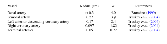
with respect to the radius of arteries in the human circulatory system are tabulated in table 1. In this study, for the Newtonian fluid flow,
 $\alpha$
is considered in the range of
 $0.1-4$
to account for the pulsatile part of the pressure gradient. However, for Casson fluid flow, we have considered
 $\alpha \ll 1$
. The Péclet number
 ${\textit{Pe}}$
is taken as
 $10^3$
throughout our calculations (Sankarasubramanian & Gill Reference Sankarasubramanian and Gill1973; Mazumder & Das Reference Mazumder and Das1992; Rana & Murthy Reference Rana and Murthy2016a
, Reference Rana and Murthy2017a
; Rana et al. Reference Rana, Das, Sarifuddin, Mandal and Patne2024). The value of Schmidt Number
 $Sc$
is
 $O(10^3)$
in the arterial blood flow, and it is given as
 $10^3$
(Caro Reference Caro2012; Rana & Murthy Reference Rana and Murthy2017a
). The oscillatory Péclet number
 $P^2_{\omega }$
is considered in the range of
 $10-16000$
based on the values of
 $\alpha$
and
 $Sc$
(Keith Sharp, Carare & Martin Reference Keith Sharp, Carare and Martin2019; Singh & Murthy Reference Singh and Murthy2023; Rana et al. Reference Rana, Das, Sarifuddin, Mandal and Patne2024). For the steady flow, the amplitude of the fluctuating pressure component
 $e=0$
is considered, and for a pulsatile flow,
 $e$
is taken as
 $0.2$
for a healthy human adult from the standard blood pressure
 $120/80$
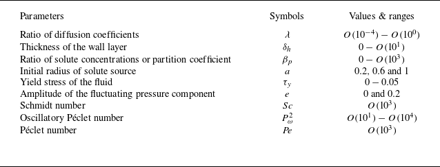
mm Hg (Rana et al. Reference Rana, Das, Sarifuddin, Mandal and Patne2024). In addition, all these relevant ranges of the dimensionless parameters are tabulated in table 2 for the better understanding of readers.
The ranges and values of the dimensionless parameters relevant to the present study.

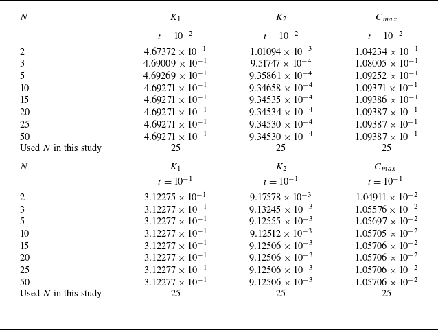
Convergence analysis of the transport coefficients
 $K_i(t)\,(i=1,2)$
and the mean concentration
 $\overline {C}$
based on the series terms used in the computation. The value
 $N\in \mathbb{N}$
is the total number of roots
 $\mu _{n}$
in the transcendental (3.17). The coefficients
 $K_1(t)$
and
 $K_2(t)$
can be expressed in the terms of partial sums as
 $K_1(t):=\sum _{n=0}^{N} A_{n}(t) =S_N(t)$
and
 $K_2(t):=\sum _{n=0}^{N}\sum _{m=0}^{N} B_{nm}(t)+\sum _{n=0}^{N} C_n(t)=T_{N}(t)$
, respectively. Note that the sequences of the partial sums,
 $\{S_N(t)\}$
and
 $\{T_N(t)\}$
, converge to the corresponding infinite series sum as
 $N\rightarrow \infty$
. Applying the Cauchy criterion for series convergence, we have
 $\forall \, t\gt 0$
and for any
 $\epsilon \gt 0$
,
 $\exists \,\, N_0\in \mathbb{N}$
(
 $N_0$
depends on
 $\epsilon$
), such that
 $|S_{N+P}(t)-S_{N}(t)|\lt \epsilon$
and
 $|T_{N+P}(t)-T_{N}(t)|\lt \epsilon$
,
 $\forall \, N\geqslant N_0$
and
 $P\in \mathbb{N}$
. Here,
 $N_0$
is taken sufficiently large (i.e.
 $N_0=25$
) to achieve the high numerical accuracy having very small
 $\epsilon$
. This criterion confirms that the series for each
 $K_i(t)$
is convergent. Since the mean concentration
 $\overline {C}$
depends directly on
 $K_1$
and
 $K_2$
, it also converges for sufficiently large
 $N_0\geqslant 25$
. In this study, we have adopted the Simpson’s
 $1/3$
rule of integration to compute the integrals numerically. The time interval
 $[0,t]$
is divided into an even number of
 $M$
subintervals by
 $(M+1)$
grid points with equal step size
 $h=t/M$
. For high accuracy, we have considered
 $M\geqslant 150$
. These results are computed for the steady flow of Newtonian fluid when
 $e=0$
,
 $a=1$
,
 $\beta _{p} =10$
,
 $\lambda =0.8$
,
 $P^2_{\omega }=1$
,
 ${\textit{Pe}}=10^3$
and
 $R=1.1$
.

4.2. Validation of the study
In this study, to check the accuracy of our results, we have performed the convergence analysis for the transport coefficients
 $K_i(t)$
 $(i=1,2)$
and mean concentration
 $\overline {C}(t,x)$
. The details are provided in table 3. In addition, to check the accuracy of this analysis, we have compared our results with those obtained by Phillips et al. (Reference Phillips, Kaye and Robinson1995) for the steady flow of Newtonian fluid, considering the small values of
 $\lambda$
and
 $\delta _{h}\, (\ll 1)$
. Following the study of Phillips et al. (Reference Phillips, Kaye and Robinson1995), we have denoted
 $\kappa$
as an absorption parameter, which is defined by
 $\sqrt {\lambda }\,\beta _{p}$
. The value of
 $\kappa$
is considered in the range of
 $10^{-2}-10$
to compare with the results of Phillips et al. (Reference Phillips, Kaye and Robinson1995). The variation of convection coefficient
 $K_1$
and convective component of the dispersion coefficient
 $K_c(t)$
with time
 $t$
is plotted for select values of
 $\kappa$
and is shown in figure 2. These results are in excellent agreement with Phillips et al. (Reference Phillips, Kaye and Robinson1995). To ensure the accuracy of our results for pulsatile, non-Newtonian fluid flow, we have further validated the single-phase (fluid-only) limit of our model by comparing it with the results reported in Rana & Murthy (Reference Rana and Murthy2016a
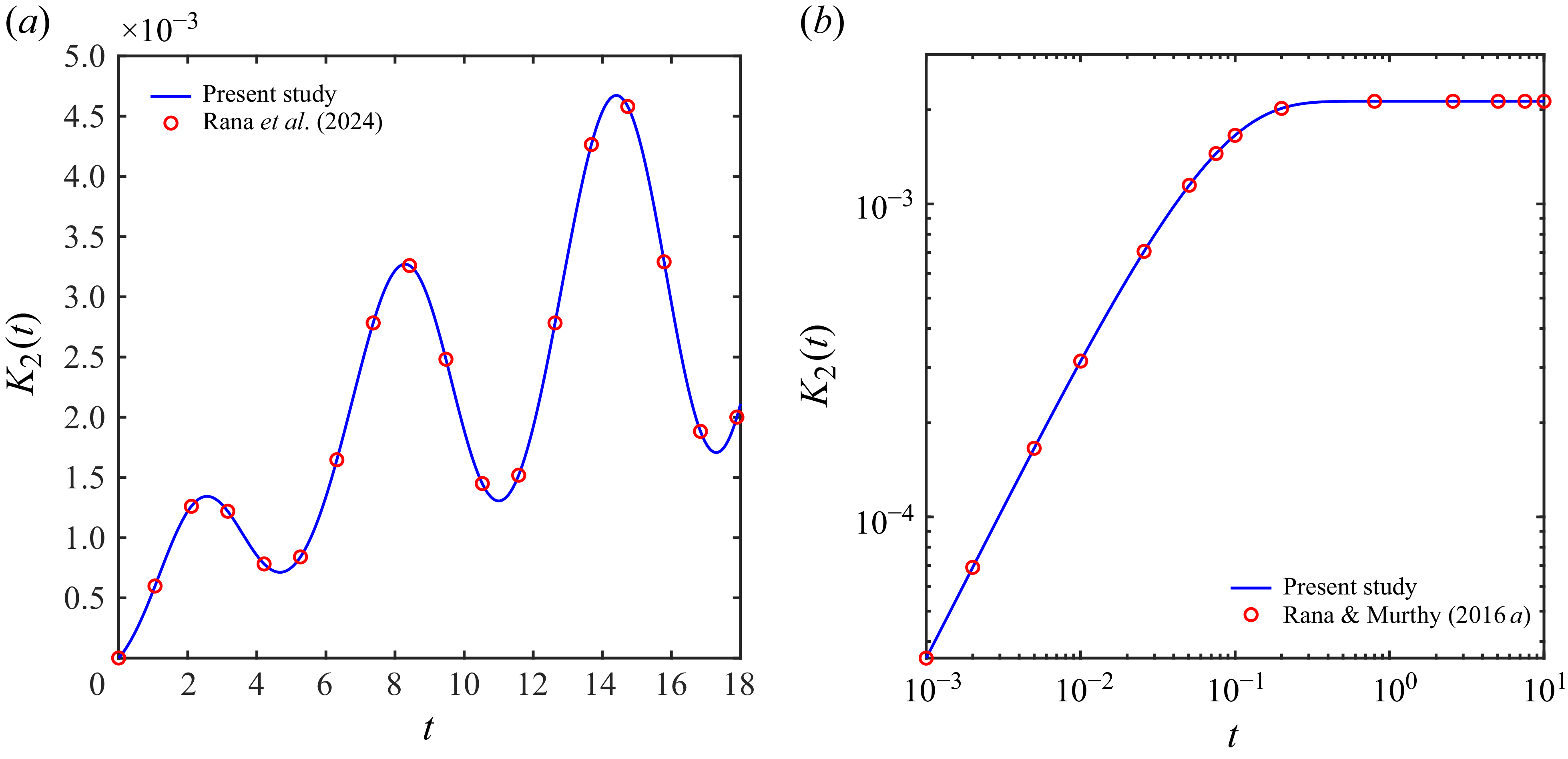
) and Rana et al. (Reference Rana, Das, Sarifuddin, Mandal and Patne2024). From figure 3, these results agree well with Rana & Murthy (Reference Rana and Murthy2016a
) and Rana et al. (Reference Rana, Das, Sarifuddin, Mandal and Patne2024), thereby validating our solution procedure. For the ease of presenting the results, we divide the subsequent discussion into separate sections dealing with Newtonian (
 $\tau _{y}=0$
) and Casson (
 $\tau _{y}\neq 0$
) fluids.
Validation of our methodology by comparing our results with those of Phillips et al. (Reference Phillips, Kaye and Robinson1995) in the steady flow of Newtonian fluid for select values of absorption parameter
 $\kappa =\sqrt {\lambda }\,\beta _p$
, when
 $a=1$
,
 $\lambda =10^{-4}$
,
 $e=0$
,
 $P^2_{\omega }=1$
and
 $R=1.1$
. Here, the velocity profile for steady Newtonian fluid flow is given by
 $w(r)=2\,(1-r^2)$
. (a) For the convection coefficient and (b) for the convective component of the dispersion coefficient.

Validation of our methodology by comparing our results for dispersion coefficient
 $K_2(t)$
with those of Rana et al. (Reference Rana, Das, Sarifuddin, Mandal and Patne2024) and Rana & Murthy (Reference Rana and Murthy2016a
) in the limit of
 $\delta _{h}\rightarrow 0$
, i.e. in the context of single phase (fluid phase only). Panel (a) is for the pulsatile flow of Newtonian fluid when
 $e=0.5$
,
 $\alpha =0.5$
,
 $a=1$
,
 $P^2_{\omega }=250$
,
 ${\textit{Pe}}=10^3$
,
 $R=1$
and
 $\tau _y=0$
, and panel (b) is for the steady flow of Casson fluid when
 $e=0$
,
 $P^2_{\omega }=1$
,
 ${\textit{Pe}}=10^3$
,
 $a=1$
,
 $R=1$
and
 $\tau _y=0.05$
.

4.3. Newtonian fluid (
 $\tau _{y}=0$
)

The following discussion elaborates the impact of
 $\lambda$
,
 $\beta _{p}$
,
 $\delta _{h}$
and
 $a$
on solute convection, dispersion and concentration distribution based on averages over fluid and wall phases at short and long time scales in both steady and pulsatile flows.
4.3.1. Effect of
$\lambda$

Figure 4(a) shows the effect of
 $\lambda$
on the convection coefficient
 $K_1$
over short and long time scales, considering the steady flow of Newtonian fluid. To provide a ready comparison, we have considered
 $\lambda =10^{-4}$
given in the study of Phillips et al. (Reference Phillips, Kaye and Robinson1995) and extended to
 $\lambda =1$
, relevant to solute transport in blood flow. After the injection of the solute in the fluid phase, initially (at
 $t=0$
), the solute is convected with the mean velocity of the fluid phase for all
 $\lambda$
, implying
 $K_1=-1/2$
 $\forall \,\, \lambda$
as shown in figure 4(a). However, after
 $t\gt 0$
, for high values of
 $\lambda$
,
 $K_1$
decreases rapidly in the short time regime and reaches a constant value quickly in the large time limit. The physical reason is explained as follows.
Temporal variation of convection coefficient
 $K_1$
for select values of
 $\lambda$
in the Newtonian fluid flow when
 $a=1$
,
 $\beta _{p} =10$
and
 $R=1.1$
. (a) For steady flow when
 $e=0$
and
 $P^2_{\omega }=1$
; (b) for pulsatile flow when
 $e=0.2$
,
 $\alpha =0.1$
and
 $P^2_{\omega }=10$
.

At time
 $t=0$
, the solute remains in the fluid phase only, and there is no solute in the wall phase. Thus, the solute is convected with the average velocity of the fluid in agreement with the previous studies dealing with the solute dispersion in a steady pipe flow (Sankarasubramanian & Gill Reference Sankarasubramanian and Gill1973). However, for
 $t\gt 0$
, the solute from the slow-moving fluid flow region near the fluid–wall interface enters the wall layer, thereby moving out of the fluid phase and increasing the solute fraction in the wall phase. Note that the transport coefficients are calculated based on the averages over both phases. Consequently, for
 $t\gt 0$
, the convection coefficient (
 $K_1$
) results from convection in both fluid and wall phases. Since there is no fluid velocity in the wall layer, convection is absent. Thus, for
 $t\gt 0$
, even as solute moves from the fluid phase to the wall phase, solute convection occurs only in the fluid phase. The solute concentration is decreasing in the fluid phase due to continuous transfer from fluid to wall, implying that an increasingly lower amount of solute is being convected, resulting in decreasing
 $K_1$
with time. In the large time limit, the solute exchange between the fluid and wall phases reaches an equilibrium based on the solute diffusivities in the fluid and wall phases, i.e.
 $\lambda$
. As
 $\lambda$
increases, the resistance offered by the wall phase for the solute diffusion reduces, which enhances the solute transfer from fluid to wall. This enhancement then hastens the solute equilibrium between two phases, and the concentration in the fluid reaches a constant value as shown in figure 4(a).
To determine the large-time behaviour of
 $K_1$
, the asymptotic expression is determined by considering
 $t\rightarrow \infty$
. This will provide a clear understanding of the long-time behaviour of the dispersion process in both phases. The large time expressions for
 $f_0(r)$
and
 $g_0(r)$
for a steady flow of Newtonian fluid are derived from (3.13) and (3.14) as
 \begin{equation} f_{0}(r) = \frac {R^2}{1+\beta _{{p}}\left (R^2-1\right )} \end{equation}
and
 \begin{equation} g_{0}(r) = \frac {R^2\beta _{{p}}}{1+\beta _{{p}}\left (R^2-1\right )}, \end{equation}
where
 $R=1+\delta _{h}$
. The asymptotic expression of convection coefficient
 $K_1$
in both fluid and wall phases is determined as follows:
 \begin{align} \displaystyle K_{1}=-\frac {2}{R^2}\int _{0}^{1}r\,w(r)\,f_{0}(r) \,\mathrm{d} r = -\frac {\overline {w(r)}}{\left [1+\beta _{{p}}\left (R^2-1\right )\right ]} =-\frac {\kappa _{s}}{2}, \end{align}
where the average velocity
 $\overline {w(r)}$
is
 $1/2$
for Newtonian fluid and
 $\kappa _{s}$
is the steady state solute fraction in the fluid defined by
 $\kappa _{s}=1/ [1+\beta _{{p}} (R^2-1 ) ]$
. The same steady state results for
 $K_1$
can also be directly obtained from (3.19) by considering the limit
 $t\rightarrow \infty$
. From the expression of
 $K_1$
given in (4.3), at a large time scale, solute convection does not depend on the ratio of diffusion coefficients
 $\lambda$
. Consequently, for any
 $\lambda$
at large time scale,
 $K_1$
approaches to the same value of
 $- (1/2 )\kappa _{s}$
, as seen in figure 4(a). From (4.3), the asymptotic expression of
 $K_1$
is independent of the initial dimensionless radius of the solute source,
 $a$
. So, solute convection at large time scales is not affected by the non-uniformity of the initial distribution of the solute. However, the significant effect of
 $a$
on solute convection is predicted at short time scales in this study, as presented later in this section.
Note that the asymptotic
 $K_1$
depends on the ratio of solute concentrations
 $\beta _{p}$
across the fluid–wall interface and the thickness of the wall layer
 $\delta _{h}$
in terms of
 $R$
. When only the fluid phase is considered, resulting in
 $K_1$
as
 \begin{align} \displaystyle \lim _{R\to 1 \mbox{ or } \delta _{h} \to \, 0} K_{1}&=-\frac {1}{2}, \end{align}
which is the same reported in the study of Sankarasubramanian & Gill (Reference Sankarasubramanian and Gill1973). So, for a single phase, i.e. for fluid-phase only, the solute is convected at the average velocity of the fluid (Sankarasubramanian & Gill Reference Sankarasubramanian and Gill1973). In contrast, for two phases, i.e. for fluid–wall phases, the solute is convected with a much lower velocity than the average velocity of the fluid. For any
 $\lambda$
, the solute is convected with the same lower velocity of the fluid
 $0.16129$
for
 $\beta _{p}=10$
and
 $\delta _{h}=10^{-1}$
since
 $\kappa _s$
defined above is not a function of
 $\lambda$
.
The behaviour of
 $K_1$
for select values of
 $\lambda$
in the pulsatile flow is depicted in figure 4(b). As seen in the case of steady flow, barring oscillations, a similar trend for time required to achieve equilibrium is predicted in the pulsatile flow. From figure 4(b), the oscillation of
 $K_1$
exhibits a progressive decline for small values of
 $\lambda$
, whereas a sharp decrement is predicted for high values of
 $\lambda$
. In the pulsatile flow with
 $\alpha =0.1$
, the oscillation of
 $K_1$
becomes stable (i.e. of constant amplitude) at
 $t\simeq 10$
for
 $\lambda =1$
, whereas a long time of approximately
 $t\gtrsim 10^3$
is required to reach the stable state for
 $\lambda =10^{-4}$
. It suggests that more time is required to reach the stable state in the case of pulsatile flow than in the case of steady flow. By following the present results, we have predicted a relationship between the time scales for reaching the stable state regime in the steady and pulsatile flows, and it is defined by
 $t_{p} \simeq P^2_{\omega }\,t_{s}$
, where
 $t_{p}$
and
 $t_{s}$
denote the dimensionless times for pulsatile and steady flows, respectively, where
 $P^2_{\omega }$
is the oscillatory Péclet number.
Temporal variation of dispersion coefficient
 $K_2$
with
 $t$
for select values of
 $\lambda$
. Panel (a) is for the steady flow of Newtonian fluid when
 $a=1$
,
 $\beta _{p} =10$
,
 $e=0$
,
 $P^2_{\omega }=1$
and
 $R=1.1$
. Panels (b) and (c) are for the pulsatile Newtonian fluid flow at
 $a=1$
,
 $\beta _{p} =10$
,
 $e=0.2$
,
 $\alpha =0.1$
and
 $P^2_{\omega }=1$
at small and large time scales, respectively.

The variation of
 $K_2$
for select values of
 $\lambda$
with time is depicted in figure 5(a) for steady flow. From figure 5(a), for all
 $\lambda$
values,
 $K_2$
rapidly increases up to a certain time (depending on
 $\lambda$
value) but attains a constant magnitude in the large time limit. This large time value inversely varies with
 $\lambda$
value. Further, for
 $\lambda =1$
,
 $K_2$
goes through a peak value such that the large time
 $K_2$
value is less than peak value.
At
 $t=0$
, the solute is uniformly distributed over the cross-section of the tube in the fluid phase. For
 $t\gt 0$
, it moves downstream with the velocity of the fluid and starts to spread axially. The shape of the solute turns into the shape of the velocity profile. This convective transport induced by the velocity gradient over the cross-section of the tube enhances solute dispersion. At the same time, interphase mass transfer initiates the exchange of the solute between the two phases, thereby triggering radial diffusion at the front and rear fractions of the solute cloud within the fluid phase. Notably, the rear portion contributes the most to the interphase transfer of the solute to the wall region. The radial diffusion from the fluid–wall interface region (low fluid velocity region) to the central region of the tube (high fluid velocity region) is impeded by the exchange process. Note that in the wall phase, solute dispersion occurs solely through diffusive transport, whereas in the fluid phase, both shear flow and diffusion jointly contribute to solute spreading. Since
 $\lambda =1$
implies a comparable molecular diffusivity in the wall and fluid phases, the solute diffuses more quickly across the wall layer compared with smaller values of
 $\lambda$
. Consequently, the equilibrium state for the diffusion process is achieved faster for large
 $\lambda$
than for small
 $\lambda$
.
From figure 5(a), at large times, the solute dispersion is higher for small
 $\lambda$
due to a higher
 $K_2$
value. Physically, this could be explained as follows. For small values of
 $\lambda$
, the diffusive process in the wall phase is slower due to lower values of molecular diffusivity. Owing to this, the solute leaves the fluid phase gradually, and a larger amount of solute remains in the fluid phase, in comparison with large
 $\lambda$
. The solute convection becomes higher for small
 $\lambda$
as discussed earlier, and it plays a strong supportive role in the dispersion process over longer durations since
 $K_2$
for the fluid phase depends on
 $K_1$
. In addition, the fluid phase exhibits comparatively higher diffusivity than the wall phase for a smaller
 $\lambda$
. For higher values of
 $\lambda$
an opposite scenario exists. Note that
 $K_2$
is a phase-averaged quantity in fluid and wall phases. Since for small
 $\lambda$
a higher solute is present in the fluid phase, the combined effect of shear-enhanced dispersion and strong molecular diffusivity enhances axial dispersion of the solute in the fluid phase, leading to a significant enhancement of total
 $K_2$
. A similar set of arguments implies that
 $K_2$
should be lower for higher
 $\lambda$
. This is indeed the case shown in figure 5(a).
We have determined the large time expression for
 $K_2$
in the steady flow. By taking
 $t\rightarrow \infty$
, (3.9a
) and (3.9b
) for
 $k=1$
are solved to obtain
 $f_1(r)$
and
 $g_1(r)$
as
 \begin{align} \displaystyle f_1(r) &= -\frac {1}{48 \lambda \left (\beta _{p} \left (R^2-1\right )+1\right )^3}\,\Bigg [R^2 \bigg (3 \,\beta _{p}^2 \,\lambda \left (\!r^4-4\, r^2+3\!\right ) \left (\!R^2-1\!\right )^2+\beta _{p} \left (\!R^2-1\!\right )\nonumber \\ &\quad\times\Big (2 \lambda \left (3 r^4-9 r^2+4\right )-9 R^2+3\Big )+12 \beta _{p} R^4 \log (R)+\lambda \left (3 r^4-6 r^2+2\right )\!\bigg )\Bigg ] \end{align}
and
 \begin{align} & g_1(r)= \frac {1}{48 \lambda \left (\beta _{p} \left (R^2-1\right )+1\right )^3}\Bigg [\beta _{p} R^2 \bigg (4 \beta _{p} \lambda R^2-4 \beta _{p} \lambda -6 \beta _{p} r^2 R^2+6\beta _{p} r^2+12 R^2\nonumber \\ &\times \!\Big (\beta _{p} \left (\!R^2-1\!\right )+1\!\Big )\! \log (r)+9 \beta _{p} R^4-12 \beta _{p} R^4 \log (R)-6 \beta _{p} R^2-3 \beta _{p}+\lambda -6 r^2+6\!\bigg )\!\Bigg ], \end{align}
respectively. The large time expression of the dispersion coefficient
 $K_2$
is
 \begin{align} &K_2=\displaystyle \frac {\lambda }{{\textit{Pe}}^2}+\frac {2}{R^2}\frac {\left (1-\lambda \right )}{{\textit{Pe}}^2}\,\int _{0}^{1}r\,f_{0}(r)\,\mathrm{d} r-\frac {2}{R^2}\int _{0}^{1}r\,w(r)\,f_{1}(r) \,\mathrm{d} r\nonumber \\ &=\frac {\lambda }{{\textit{Pe}}^2}+\frac {(1-\lambda )}{{\textit{Pe}}^2} \frac {1}{1+\beta _{{p}}\left (\!R^2-1\!\right )}+\frac {1}{192\,\left (\beta _{p} \left (\!R^2-1\!\right )+1\!\right )^3}+\frac {1}{192\, \lambda \left (\beta _{p} \left (\!R^2-1\!\right )+1\!\right )^3}\nonumber \\ &\quad\times \Big [11\, \beta _{p}^2 \,\lambda \Big (\!R^2-1\!\Big )^2+6 \,\beta _{p} \,\left (\!R^2-1\!\right ) \left (\!\lambda -3 R^2+1\!\right )+24 \,\beta _{p}\, R^4\, \log (R)\Big ]. \end{align}
From the right-hand side of (4.7), the first two terms are the diffusive component of
 $K_2$
and the last two terms are the convective component of
 $K_2$
, i.e. the shear-enhanced dispersion occurring due to the velocity gradient in the fluid phase. The diffusive component of
 $K_2$
can also be directly obtained from (3.26) after taking
 $t\rightarrow \infty$
, i.e.
 $\displaystyle {\lim _{t \to \, \infty } K_{d}(t)}$
. From (4.7), at long time scales, the solute dispersion depends on the parameters
 $\lambda$
,
 $\beta _{p}$
and
 $\delta _{h}$
(in terms of
 $R$
). Considering only the fluid phase,
 $K_2$
is reduced to
 \begin{align} \displaystyle {\lim _{R\to 1 \mbox{ or } \delta _{h} \to \, 0} K_2=\frac {1}{{\textit{Pe}}^2}+\frac {1}{192}}, \end{align}
which is the same as calculated by Sankarasubramanian & Gill (Reference Sankarasubramanian and Gill1973). For
 $\lambda =1$
, the steady state reaches quickly at
 $t\simeq 1$
and attains a value
 $1.0921\times 10^{-2}$
in the long time limit. For
 $\lambda =10^{-4}$
, it is approximately
 $10^2$
owing to the prolonged time scales for diffusive processes in the wall phase, and
 $K_2$
attains a constant value
 $6.2708\times 10^{-1}$
. Note that in the absence of the wall phase, the steady-state regime for dispersion reaches at
 $t\simeq 0.5$
with
 $K_2 = 5.2093\times 10^{-3}$
(Sankarasubramanian & Gill Reference Sankarasubramanian and Gill1973; Rana & Murthy Reference Rana and Murthy2016a
), which is lower than that in the case of two phases. The present results of
 $K_2$
for select
 $\lambda$
predict that solute exchange between two phases enhances the dispersion averaged over both phases
 $ (K_2\sim O(10^{-2})-O(10^{-1}) )$
compared with that without solute exchange
 $ (K_2\sim O(10^{-3}) )$
. In addition, the steady state regime for dispersion is prolonged for solute exchange
 $ ( t \sim O(10^0)-O(10^2) )$
than in the case without exchange
 $ ( t \sim 0.5 )$
, depending on
 $\lambda$
. From (4.7), the asymptotic expression of
 $K_2$
is independent of
 $a$
. Thus, solute dispersion at large time scales is not influenced by the non-uniformity of the initial distribution of the solute. However, the substantial effect of
 $a$
on solute dispersion is predicted at short time scales in this study, as presented later in this section.
The effect of
 $\lambda$
on
 $K_2$
is shown in figure 5 for pulsatile flow. The similar behaviour of
 $K_2$
with
 $\lambda$
is seen for pulsatile flow, as discussed for steady flow. The oscillation amplitude of
 $K_2$
increases with
 $\lambda$
at short times, whereas at long times, constant amplitude oscillations exist. For
 $\alpha =0.1$
and
 $\lambda =1$
,
 $K_2$
reaches a constant amplitude state at
 $t\simeq 10$
, whereas for
 $\lambda =10^{-4}$
, this state is achieved after a long time
 $t\simeq 10^{3}$
. Similar to convection coefficient, the constant amplitude state for solute dispersion is achieved with a later for pulsatile flow compared with steady flow.
4.3.2. Effect of
$\beta _{p}$

The parameter
 $\beta _{p}$
is partition coefficient, i.e. thermodynamically,
 $\beta _{p}$
determines the fractions of total solute concentration present in the fluid and wall layer at equilibrium. Figure 6 shows the effect of
 $\beta _{p}$
on variation of convection coefficient
 $K_1$
with time for steady and pulsatile flows of a Newtonian fluid. From figure 6(a), as
 $\beta _{p}$
increases,
 $K_1$
decreases sharply at short times and reaches the steady state at long times. Physically, this could be explained as follows.
For small values of
 $\beta _{p}$
, the solute fraction in the wall phase is small compared with that in the fluid phase. That means a very small fraction of the solute is transported to the wall phase across the fluid–wall interface and most of the solute is retained by the fluid phase. The parameter
 $K_1$
is the transport of the solute weighted by the fluid velocity due to the absence of convection in the wall phase. Due to a small loss of the solute from the fluid to wall,
 $K_1$
remains largely unaffected for
 $\beta _p=0.1$
(see figure 6
a). However, for large values of
 $\beta _{p}$
, a higher fraction of solute is transferred from the fluid phase to the wall phase. This higher transfer of solute amount could explain the higher time requirement to reach steady state for an increasing
 $\beta _{p}$
.
Temporal variation of convection coefficient
 $K_1$
with
 $t$
for select values of
 $\beta _{p}$
in the Newtonian fluid flow when
 $a=1$
,
 $\lambda =0.8$
and
 $R=1.1$
. Panel (a) is for steady flow when
 $e=0$
and
 $P^2_{\omega }=1$
and panel (b) is for pulsatile flow when
 $e=0.2$
,
 $\alpha =0.1$
and
 $P^2_{\omega }=10$
.

For
 $\beta _{p}=10^{-1}$
, the solute convection reaches the steady state at
 $t\simeq 0.5$
, whereas for
 $\beta _{p}=10^{2}$
, it reaches over the long time regime
 $(t\gtrsim 2)$
. Unlike for
 $\lambda$
, the significant differences in
 $K_1$
with respect to
 $\beta _{p}$
are predicted at large time scales, since the asymptotic expression for
 $K_1$
(see (4.3)) strongly depends on
 $\beta _{p}$
. Note that asymptotic
 $K_1$
is inversely proportional to
 $\beta _{p}$
. For
 $\beta _{p}=0, 10^{-1}, 1, 10$
and
 $10^2$
, the steady state constant magnitudes of
 $K_1$
are
 $0.5, 0.4897, 0.4132, 0.1613$
and
 $0.0227$
, respectively. Similar decreasing trends in
 $K_1$
with increasing wall absorption parameter
 $\kappa =\sqrt {\lambda }\,\beta _{p}$
for
 $\lambda =10^{-4}$
are reported by Phillips et al. (Reference Phillips, Kaye and Robinson1995) (see figure 2
a).
(a) Temporal variation of dispersion coefficient
 $K_2$
with
 $t$
for select values of
 $\beta _{p}$
in the steady flow of Newtonian fluid when
 $a=1$
,
 $e=0$
,
 $P^2_{\omega }=1$
,
 $\lambda =0.8$
and
 $R=1.1$
; (b) temporal variation of dispersion coefficient
 $K_2$
with
 $t$
for select values of
 $\beta _{p}$
in the pulsatile flow of Newtonian fluid when
 $a=1$
,
 $e=0.2$
,
 $\alpha =0.1$
,
 $P^2_{\omega }=10$
,
 $\lambda =0.8$
and
 $R=1.1$
; (c) the variation of asymptotic dispersion coefficient
 $K_2$
at very long time scales with
 $\beta _{p}$
for select values of
 $\lambda$
in the steady flow of Newtonian fluid when
 $e=0$
,
 $P^2_{\omega }=1$
and
 $R=1.1$
.

From figure 6(b), a similar effect of
 $\beta _{p}$
on
 $K_1$
is predicted in the pulsatile flow. The oscillation of
 $K_1$
decreases slowly for small values of
 $\beta _{p}$
, whereas a significant decrement is seen for large
 $\beta _{p}$
. The oscillations become stable for
 $t\gtrsim 5$
for
 $\beta _{p}=10^{-1}$
and for
 $t\gtrsim 20$
for
 $\beta _{p}=10^{2}$
.
Figure 7 illustrates the behaviour of
 $K_2$
with select values of
 $\beta _{p}$
for both steady and pulsatile flows. From figure 7(a), for small values of
 $\beta _{p}$
,
 $K_2$
increases at small times and reaches a stable state at large times. However, for high values of
 $\beta _{p}$
, a contrasting behaviour is predicted in the moderate and large times. In this case,
 $K_2$
increases at short times and decreases sharply at moderate times. Thereafter, it becomes stable with a lower constant value in the long-time regime. Physically, this behaviour could be explained as follows.
For
 $\beta _p=10^{-2}$
, the wall phase has a minor effect on
 $K_2$
since most of the solute is retained by the fluid phase. In this case, the system behaves as a fluid flow through a pipe as shown by the red dotted curve in figure 7(a). As
 $\beta _p$
increases, the wall phase increasingly retains more solute. At
 $\beta _p=1$
both fluid and wall phases are equally preferred by the solute. However, in the wall phase, only molecular diffusion is possible while convective solute transfer or shear-enhanced dispersion is absent. Due to
 $\beta _p=1$
, to achieve the same solute fractions in fluid and wall phases, diffusion in the wall phase must exhibit a similar order of solute movement as in the fluid phase by using diffusion alone. This requires a considerably higher diffusion in the wall phase. Additionally, the solute in the fluid phase is rapidly transported near the fluid–wall interface by shear-enhanced dispersion and molecular diffusion. Since
 $K_2$
is a phase-averaged quantity which accounts for dispersion in both fluid and wall phases, the enhanced dispersion in the wall and fluid phases increases the
 $K_2$
value. Due to this, for
 $\beta _p=1$
,
 $K_2$
is higher than for flow through a pipe without a wall phase.
As
 $\beta _p$
increases beyond unity, the solute preference tilts in favour of the wall phase as a larger solute fraction is retained by the wall phase at equilibrium. Thus, as soon as solute is injected in the fluid phase, solute prefers to move to wall phase as the wall phase acts as a strong mass sink. This leads to a rapid increase in the dispersion in both phases due to the rapid transfer of the solute from the fluid phase (source) to the wall phase (sink). This transfer reaches its peak when the thermodynamically feasible partition of the solute is reached, signified by a peak in green and magenta curves shown in figure 7(a). As soon as the solute transfer peak is over, owing to the absence of shear-enhanced dispersion in the wall phase where most of the solute is located,
 $K_2$
, which denotes the dispersion in both phases, starts to decrease. The steady state value of
 $K_2$
largely depends on the fraction of the solute present in the fluid phase, where shear-enhanced dispersion drastically enhances
 $K_2$
. For increasing
 $\beta _p$
, a decreasing solute fraction is present in the fluid, thus an increasing fraction of the solute misses the shear-enhanced dispersion. This could explain the rapid decrease in the green curve shown in figure 7(a). From figure 7(b), similar arguments could be used for the pulsatile flow of Newtonian fluid. The oscillation of
 $K_2$
increases as
 $\beta _{p}$
increases. However, for very high values of
 $\beta _{p}$
, it decreases significantly at long time scales. For
 $\beta _{p}=10^{-2}$
, the oscillations become stable after
 $t\gtrsim 5$
, whereas it occurs after
 $t\gtrsim 20$
for
 $\beta _{p}=10^{2}$
.
From figure 7(c), the asymptotic
 $K_2$
is plotted with
 $\beta _{p}$
for select values of
 $\lambda$
at very large times. As
 $\beta _{p}$
increases,
 $K_2$
increases for small
 $\beta _{p}$
and reaches its maximum peak value at a certain
 $\beta _{p}$
, and thereafter, it decreases sharply for large
 $\beta _{p}$
. As discussed earlier, solute dispersion decreases as
 $\lambda$
increases. The maximum peak of
 $K_2$
reaches a small
 $\lambda =10^{-4}$
. For small
 $\lambda$
and
 $\beta _{p}$
, the combined action of the shear flow and the high rate of diffusion in the fluid phase leads to the enhancement of axial spreading in the fluid phase. However, for high values of
 $\beta _{p}$
, the opposite scenario arises, and the physical reason for decreasing
 $K_2$
is stated above. A similar long-time behaviour is predicted for other values of
 $\lambda$
. In addition, the critical value of
 $\beta _{p}$
at which
 $K_2$
attains the maximum peak increases with increasing
 $\lambda$
. Note that, after this critical value of
 $\beta _{p}$
,
 $K_2$
diminishes with increasing
 $\beta _{p}$
. For
 $\lambda =10^{-4}, 10^{-3}, 10^{-2}$
and
 $1$
,
 $K_2$
reaches its maximum peak value
 $1.3055,0.13997,0.02372$
and
 $0.01187$
when
 $\beta _{p}=2.3884,2.4552,3.0722$
and
 $5.3943$
, respectively. These findings offer valuable insight into optimising the solute exchange across the fluid–wall interface to achieve maximum dispersion. As discussed earlier, the solute exchange process enhances the dispersion
 $ (K_2\sim O(10^{-3})-O(10^{0}) )$
and reaches the steady state at prolonged time scales
 $ (t\sim O(10^{-1})-O(10^{0}) )$
depending on
 $\beta _{p}$
.
Temporal variation of convection coefficient
 $K_1$
with
 $t$
for select values of
 $\delta _{h}$
in the terms of
 $R=1+\delta _{h}$
in the Newtonian fluid flow when
 $a=1$
,
 $\lambda =0.8$
and
 $\beta _{p}=10$
. Panel (a) is for steady flow when
 $e=0$
and
 $P^2_{\omega }=1$
and panel (b) is for pulsatile flow when
 $e=0.2$
,
 $\alpha =0.1$
and
 $P^2_{\omega }=10$
.

(a) Temporal variation of dispersion coefficient
 $K_2$
with
 $t$
for select values of
 $\delta _{h}$
in the terms of
 $R=1+\delta _{h}$
in the steady flow of Newtonian fluid when
 $a=1$
,
 $\lambda =0.8$
,
 $\beta _{p}=10$
,
 $e=0$
and
 $P^2_{\omega }=1$
; (b) temporal variation of dispersion coefficient
 $K_2$
with
 $t$
for select values of
 $\delta _{h}$
in the terms of
 $R=1+\delta _{h}$
in the pulsatile flow of Newtonian fluid when
 $a=1$
,
 $\lambda =0.8$
,
 $\beta _{p}=10$
,
 $e=0.2$
,
 $\alpha =0.1$
and
 $P^2_{\omega }=10$
; (c) the variation of asymptotic dispersion coefficient
 $K_2$
with
 $\beta _{p}$
for select values of
 $\delta _{h}$
in the terms of
 $R=1+\delta _{h}$
at very long time scales in the steady flow of Newtonian fluid when
 $\lambda =0.8$
,
 $e=0$
and
 $P^2_{\omega }=1$
.

4.3.3. Effect of
$\delta _{h}$

From figures 8(a) and 8(b), solute convection reduces considerably at long time scales with increasing
 $\delta _{h}$
. For very small values of
 $\delta _{h}$
, the inner tube of the fluid phase is surrounded by a thin wall layer. Solute convection is mainly weighted in favour of the fluid phase (having non-zero velocity) rather than the thin wall phase (having no fluid velocity). Due to this, the solute is convected with the fluid velocity slightly lower than the average velocity of the fluid, leading to a lower
 $K_1$
magnitude compared with the flow without the wall phase. Owing to the thin wall, the equilibrium is reached quickly. For higher values of
 $\delta _{h}$
, a larger fraction of the cross-section of the pipe is occupied by the wall phase. Thus, solute convection, mainly induced by the fluid velocity in the fluid phase, is absent in the majority of the tube cross-section. Since
 $K_1$
is a phase-averaged quantity over both phases and owing to a thick wall layer, convection in the larger cross-section of the tube is absent, resulting in the lower magnitude of
 $K_1$
with increasing
 $\delta _h$
.
In the steady flow, for
 $\delta _{h}=10^{-2}$
, the steady state is reached at
 $t\simeq 0.5$
, whereas for
 $\delta _{h}=2$
, it is delayed to
 $t\simeq 4$
. For
 $\delta _{h}=10^{-2}, 10^{-1}, 1$
and
 $2$
, the constant magnitudes of
 $K_1$
at long time scales are
 $0.4163,0.1613, 0.01613$
and
 $0.006173$
, respectively. So, the solute is convected with a much lower velocity of the fluid than the average velocity of the fluid
 $(i.e., 0.5)$
. In the pulsatile flow, oscillations in
 $K_1$
amplitude become stable after
 $t\sim 5$
for
 $\delta _{h}=10^{-2}$
and it is approximately
 $t\sim 40$
for
 $\delta _{h}=2$
.
The variation of
 $K_2$
with time for select values of
 $\delta _{h}=10^{-2}$
is shown in figure 9 for both steady and pulsatile flows. From figures 9(a) and 9(b), at short times, there is no significant effect on
 $K_2$
of
 $\delta _{h}$
variation. However, for
 $\delta _{h}\gt 0.1$
,
 $K_2$
increases with time and attains a peak value at an intermediate time, thereafter it decreases and reaches a constant value in the long time limit. For high values of
 $\delta _{h}$
, a substantial decrease in
 $K_2$
is predicted in the long-time regime compared with the peak value. This behaviour is very similar to that shown for an increasing
 $\beta _p$
shown in figure 7. In this case, an increasing
 $\delta _h$
reinforces the tendency of the wall layer to retain higher solute at equilibrium (since
 $\beta _p\gt 1$
in figure 9) by occupying an increasingly higher cross-section of the tube.
Owing to
 $\beta _p\gt 1$
, initially, the solute rapidly moves towards the wall layer to bring about thermodynamically enforced partition of solute. However, once that goal is achieved, a higher solute fraction is in the wall phase, and solute movement slows down, leading to a downward trend after the peak as shown in figure 9(a). Note that
 $K_2$
depends on the fraction of the cross-section occupied by the fluid phase, where
 $K_2$
is higher than in the wall phase owing to the shear-enhanced dispersion in the former. Thus, an increasing wall thickness, i.e.
 $\delta _h$
will decrease the region with shear-enhanced dispersion, thereby resulting in a decreasing
 $K_2$
for increasing
 $\delta _h$
. This could explain lower values of
 $K_2$
in the large time limit for
 $\delta _h\geqslant 1$
shown in figure 9(a). Since the diffusion process is the only transport mechanism in the wall layer, it takes considerable time for high
 $\delta _{h}$
to transport the solute in the wall layer and thus to reach a steady state. This explains the longer time requirement to reach a steady state or a constant amplitude state for increasing
 $\delta _h$
in figure 9.
Figure 9(c) shows the large time asymptotic behaviour of solute dispersion with the effect
 $\beta _{p}$
and
 $\delta _{h}$
. As
 $\delta _{h}$
increases,
 $K_2$
increases at small values of
 $\beta _{p}$
and attains a maximum peak value of
 $K_2$
at smaller
 $\beta _{p}$
. However, after a certain
 $\beta _{p}$
,
 $K_2$
decreases drastically with
 $\beta _{p}$
and reaches a minimum value for high
 $\delta _{h}$
and
 $\beta _{p}$
. These observations could be understood by combining the arguments utilised to explain the role of
 $\beta _p$
and
 $\delta _h$
in the preceding discussion.
4.3.4. Effect of
$\alpha$

Now, we will discuss the pulsatility effect characterised by Womersley frequency number,
 $\alpha =\hat {R_{c}}\sqrt {\hat {\omega } / (\hat {\mu }/\hat {\rho } )}$
, on solute convection and dispersion. The parameter
 $\alpha$
represents the ratio of unsteady inertial forces due to the pulsatile part of the pressure gradient to viscous forces, serving as a key parameter in characterising the impact of unsteady pressure gradients (Loudon & Tordesillas Reference Loudon and Tordesillas1998). Alternatively,
 $\alpha$
can be interpreted as a ratio of the time scale of viscous diffusion (
 $\hat {\rho } \hat {R_{c}}^2/\hat {\mu }$
) to the time scale of pressure gradient oscillation (
 $1/\hat {\omega }$
). In the small-sized tubes, the value of
 $\alpha$
is small since
 $\alpha \sim \hat R_c$
. We consider both small and large values of
 $\alpha$
in this study to investigate solute dispersion.
Temporal variation of transport coefficients for select values of
 $\alpha$
in the Newtonian fluid flow for
 $a=1$
,
 $\lambda =0.8$
,
 $R=1.1$
,
 $e=0.2$
,
 ${\textit{Pe}}=10^3$
and
 $\beta _{p}=10$
. Panel (a) is for convection coefficient
 $K_1$
and panel (b) is for dispersion coefficient
 $K_2$
.

Temporal variation of convection coefficient
 $K_1$
with
 $t$
for select values of
 $a$
in the Newtonian fluid flow when
 $\lambda =0.8$
,
 $R=1.1$
and
 $\beta _{p}=10$
. Panel (a) is for steady flow when
 $e=0$
and
 $P^2_{\omega }=1$
and panel (b) is for pulsatile flow when
 $e=0.2$
,
 $\alpha =0.5$
and
 $P^2_{\omega }=250$
.

For
 $\alpha =0.1$
, the time scale of viscous diffusion is much smaller than the pressure gradient oscillation time scale, indicating that fluid has enough time within each oscillation cycle to adjust at all times. Due to this, as the solute is injected, it rapidly starts to move to the wall phase (note
 $\beta _p=10$
in figure 10
a). As shown in figure 10(a), for
 $\alpha =0.1$
, this task is accomplished even before the effect of the pulsatile pressure gradient part impacts the flow. As
 $\alpha$
increases, the time scales defined by pressure oscillation and viscous diffusion approach each other. This does not allow the requisite solute to be transferred to the wall phase before the impact of pulsatile pressure gradient starts affecting flow. As a result,
 $K_1$
mean value decreases, even as the oscillatory pressure gradient continues to affect the flow.
Figure 10(b) shows the variation of
 $K_2$
with time. Note that the large first peak in the
 $K_2$
curve for
 $\alpha =0.1$
is not purely due to pulsatile pressure gradient, but it is mainly a consequence of the large
 $\beta _p$
value (see figure 7
a and corresponding explanation). As the pulsatile pressure gradient starts affecting the flow, there is a dip in
 $K_2$
. However, after a couple of cycles,
 $K_2$
oscillates with a constant amplitude. As
 $\alpha$
increases, the pulsatile pressure gradient hinders
 $K_2$
increase within a cycle, which leads to the oscillations in
 $K_2$
value as it approaches oscillations with constant amplitude after a larger number of cycles compared with that for
 $\alpha =0.1$
.
4.3.5. Effect of
$a$

Figure 11(a) depicts the effect of non-uniformity of the initial solute cloud on convection of the solute in the steady flow. From figure 11(a), as
 $a$
increases,
 $K_1$
decreases in short and moderate time scales. When
 $a\lt 1$
, initially, the solute cloud in the fluid phase is far from the inner tube wall. For example, for
 $a=0.2$
, it is mainly located near the centre of the inner tube. Since the fluid moves fastest at the centre and slowest near the wall, the solute near the centre is convected faster with a higher average velocity. Note that for
 $a\lt 1$
, the solute begins to convect at a velocity higher than the average velocity of the fluid. On the other hand, when
 $a$
becomes large and the solute extends towards the wall, it is convected more slowly with the lower average velocity of the fluid. This explains why the value of
 $K_1$
decreases as
 $a$
decreases during short to moderate times. However, at large times, for any
 $a$
,
 $K_1$
attains the same value and no temporal changes are predicted since the solute cloud has spread throughout the tube. For
 $a=1$
, i.e. for uniform initial distribution of the solute, the solute starts to convect with the average velocity of the fluid and decreases thereafter owing to solute transport from the fluid phase to the wall phase. At large times, for all
 $a$
, the solute is convected with the velocity
 $\kappa _s/2$
, as given in (4.3). The same trends on
 $K_1$
are predicted for the pulsatile flow as shown in figure 11(b).
Temporal variation of dispersion coefficient
 $K_2$
with
 $t$
for select values of
 $a$
in the Newtonian fluid flow when
 $\lambda =0.8$
,
 $R=1.1$
and
 $\beta _{p}=10$
. Panel (a) is for steady flow when
 $e=0$
and
 $P^2_{\omega }=1$
and panel (b) is for pulsatile flow when
 $e=0.2$
,
 $\alpha =0.5$
and
 $P^2_{\omega }=250$
.

Temporal variation of diffusive component
 $K_d$
of the dispersion coefficient
 $K_2(t)$
with
 $t$
in the Newtonian steady fluid flow. Panel (a) is for the select values of
 $\lambda$
when
 $e=0$
,
 $P^2_{\omega }=1$
,
 $a=1$
,
 $R=1.1$
and
 $\beta _{p}=10$
; panel (b) is for select values of
 $\beta _{p}$
when
 $e=0$
,
 $P^2_{\omega }=1$
,
 $a=1$
,
 $\lambda =0.8$
,
 $R=1.1$
; panel (c) is for select values of
 $a$
when
 $e=0$
,
 $P^2_{\omega }=1$
,
 $\lambda =0.8$
,
 $R=1.1$
.

From figure 12(a),
 $K_2$
increases with increasing
 $a$
at small times. For small values of
 $a$
, the solute cloud stays close to the centre of the inner tube, covering a smaller cross-sectional area. In this region, the fluid moves faster, and the velocity gradients are smaller, which causes a smaller dispersion of the solute. However, at moderate times, a contrasting behaviour is predicted. Owing to the activation of the radial diffusive transport, the solute spreads from the lower velocity gradient region (i.e. tube centre) to the slower-moving wall layer. For small values of
 $a$
, the radial diffusion increases, which helps to distribute the solute uniformly throughout the system. At large times,
 $K_2$
attains the same value for any
 $a$
, indicating that the uniform distribution is achieved. The similar effect of
 $a$
on solute dispersion is predicted for pulsatile flow as shown in figure 12(b).
4.3.6. Effect of
$\lambda$
,
$\beta _{p}$
and
$a$
on
$K_d(t)$


From (3.26), the diffusive component of the dispersion coefficient
 $K_d(t)$
strongly depends on
 $\lambda$
,
 $\beta _{p}$
and
 $a$
. In this study, the diffusive transport of the solute is discussed with the effect of
 $\lambda$
,
 $\beta _{p}$
and
 $a$
in both fluid and wall phases. From figure 13(a),
 $K_d$
decreases significantly with time for small values of
 $\lambda$
. Initially, when the solute is introduced, a large concentration difference exists between the fluid phase and the wall phase. For small
 $\lambda$
, since the diffusivity in the fluid phase is higher than the diffusivity in the wall phase, solute diffuses rapidly within the fluid, while diffusion into the wall occurs more slowly. Initially, the strong concentration gradient between the fluid and wall promotes diffusion. As time progresses, this gradient weakens, and since the wall phase offers greater resistance to diffusion, the overall diffusive transport slows down. Hence, the contribution of the diffusive component to total dispersion gradually diminishes over time. As
 $\lambda$
increases, diffusion enhances in the wall regions, promoting strong diffusive transport across the interface. When
 $\lambda =1$
, the diffusion process becomes uniform across both regions, having equal diffusivities.
From figure 13(b), as
 $\beta _{p}$
increases,
 $K_d$
diminishes in the system. As we discussed before,
 $\beta _{p}$
represents the partition coefficient determining the solute fractions of the solute concentration present in the fluid and wall layer at equilibrium. When the partition coefficient increases, more solute stays in the slower-diffusing wall phase (since
 $\lambda \lt 1$
), so the overall diffusion process becomes weaker, and the diffusive part of the dispersion decreases.
Axial variation of mean concentration
 $\overline {C}(t,x)$
with select values of
 $\lambda$
, when
 $a=1$
,
 $e=0$
,
 $\beta _{p}=10$
,
 $R=1.1$
,
 $P^2_{\omega }=1$
and
 ${\textit{Pe}}=1000$
. Panel (a) is for
 $t=0.1$
, panel (b) is for
 $t=1$
, panel (c) is for
 $t=10$
and panel (d) is for
 $t=10^2$
.

From figure 13(c),
 $K_d$
decreases with increasing values of
 $a$
at short to moderate time scales. However, at large times,
 $K_d$
is not affected by any value of
 $a$
. In a short time, for a small
 $a$
, the solute cloud is concentrated near the centre of the tube and the occurrence of the diffusive transport across the fluid–wall interface takes some time (
 $t\sim 10^{-2}$
). However, for
 $a=1$
, since the solute is readily available to the interface, it diffuses to the wall phase from the initial time, which reflects the substantial difference in
 $K_d(t)$
at short times compared with the cases for
 $a=0.2$
and
 $a=0.6$
. From (3.25), in the expression of
 $K_2$
,
 $K_d$
is multiplied by
 $1/Pe^2$
. In the study, we consider
 ${\textit{Pe}}\gg 1$
in the context of blood flow. So,
 $1/Pe^2$
can be treated as negligibly small, resulting in the insignificant effect of
 $K_d$
on solute dispersion. However, for small values of
 ${\textit{Pe}}$
,
 $K_d$
makes an impactful contribution to the dispersion process.
Axial variation of mean concentration
 $\overline {C}(t,x)$
with select values of
 $\beta _{p}$
, when
 $a=1$
,
 $e=0$
,
 $\lambda =0.8$
,
 $R=1.1$
,
 $P^2_{\omega }=1$
and
 ${\textit{Pe}}=1000$
. Panel (a) is for
 $t=0.1$
, panel (b) is for
 $t=0.5$
, panel (c) is for
 $t=10$
and panel (d) is for
 $t=10^2$
.

The spatial variations of local concentrations
 $C_{ {f}}(t,x,r)$
and
 $C_{{w}}(t,x,r)$
in both fluid and wall regions at select time scales, when
 $a=1$
,
 $\beta _{p}=10^{-1}$
,
 $e=0$
,
 $\lambda =0.8$
,
 $R=1.1$
,
 $P^2_{\omega }=1$
and
 ${\textit{Pe}}=1000$
. Here, the radial distribution of concentrations
 $C_{\!{f}}$
and
 $C_{{w}}$
is in the interval
 $r\in [0,1]$
and
 $r\in [1,1.1]$
, respectively. Panel (a) is for
 $t=0.05$
, panel (b) is for
 $t=0.5$
, panel (c) is for
 $t=1$
and panel (d) is for
 $t=10^2$
.

4.3.7. Mean concentration and local concentration of the solute
In this section, we analyse the mean concentration
 $\overline {C}(t,x)$
averaged over two phases, and the local concentrations in the fluid phase
 $C_{\!{f}}(t,x,r)$
and in the wall phase
 $C_{{w}}(t,x,r)$
.
From figure 14, as
 $\lambda$
increases, the peak of mean concentration
 $\overline {C}(t,x)$
decreases at a short time scale, whereas it increases at a long time scale. A large
 $\lambda$
indicates higher diffusivity in the wall phase than in the fluid phase. At short times, this enhanced wall diffusivity accelerates solute dispersion, leading to a lower peak in the mean concentration profile compared with smaller
 $\lambda$
values. For large
 $\lambda$
, the tail of the solute distribution profile extends farther into the
 $x\lt 0$
region compared with small
 $\lambda$
, reflecting enhanced upstream solute transport due to greater diffusivity in the wall phase. However, at large time scales, a contrasting behaviour is predicted. For small
 $\lambda$
, the solute convection is accelerated owing to the presence of more solute in the fluid phase, and strong diffusivity in the fluid phase plays a supportive role in dispersing solute more in the fluid phase. Consequently, the solute dispersion enhances significantly at long time scales, which leads to a huge decrement in the peak of the mean concentration of the solute and more downstream spreading.
Figure 15 shows time snapshots of axial variation of mean concentration
 $\overline {C}(t,x)$
for select values of
 $\beta _{p}$
. From figure 15, as
 $\beta _{p}$
increases at
 $t=0.1$
, the peak of
 $\overline {C}(t,x)$
decreases, indicating an increased dispersion of the solute in the initial stage due to a peak in
 $K_2$
for
 $\beta _p\gt 1$
(see figure 7
a). From snapshots at
 $t=0.5,10,100$
shown in figures 15(b), 15(c) and 15(d) , the difference between peaks for various values of
 $\beta _p$
increases with time. Additionally, for lower
 $\beta _p$
, peak advances much farther in the axial direction compared with higher values of
 $\beta _p$
. This is a direct consequence of a higher
 $K_1$
for a lower
 $\beta _p$
. As discussed in the explanation for figure 6(a),
 $K_1$
increases due to an increasing amount of solute gets retained in the fluid for decreasing
 $\beta _p$
.
Axial variation of mean concentration
 $\overline {C}(t,x)$
with select values of
 $\delta _{h}$
. Panels (a) and (b) are at small
 $(t=0.1)$
and moderate
 $(t=0.5)$
time scales, when
 $e=0$
,
 $a=1$
,
 $\lambda =0.8$
,
 $\beta _{p}=10$
,
 $P^2_{\omega }=1$
and
 ${\textit{Pe}}=1000$
, respectively; panels (c) and (d) are at large time scales
 $t=10^2$
, when
 $e=0$
,
 $a=1$
,
 $\lambda =0.8$
,
 $P^2_{\omega }=1$
and
 ${\textit{Pe}}=1000$
for
 $\beta _{p}=10$
and
 $\beta _{p}=10^{-2}$
, respectively.

The spatial variation of local concentrations
 $C_{\!{f}}(t,x,r)$
and
 $C_{{w}}(t,x,r)$
in both fluid and wall regions with select
 $\delta _{h}=1$
 $(R=2)$
at large time scales
 $t=10^2$
, when
 $e=0$
,
 $a=1$
,
 $\lambda =0.8$
,
 $P^2_{\omega }=1$
and
 ${\textit{Pe}}=1000$
. Here, the radial distribution of concentrations
 $C_{\!{f}}$
and
 $C_{{w}}$
is in the interval
 $r\in [0,1]$
and
 $r\in [1,2]$
, respectively. (a) For
 $\beta _{p}=10^{-2}$
; (b) for
 $\beta _{p}=1$
; (c) for
 $\beta _{p}=10$
.

The axial and radial distribution of the solute concentration in both fluid and wall phases at short- and long-time regimes is depicted in figure 16. From figure 16, at short times, the solute follows the parabolic velocity profile of the fluid and solute diffuses in the wall layer. As time progresses, the solute spreads in both phases, but owing to
 $\beta _p\lt 1$
, a larger solute fraction is retained by the fluid. Due to the combined influence of convection and molecular diffusion in the fluid phase and molecular diffusion in the wall phase, the solute concentration gradient in the radial direction decreases with increasing time. Note that the uniformity in the radial distribution of solute concentration in the fluid phase is not achieved at
 $t=1$
(see figure 16
c), and it takes a longer time
 $(t\simeq 10^2)$
(see figure 16
d), whereas the same is achieved at
 $t\simeq 1$
in the wall phase. Thus, the wall phase achieves radial uniformity much earlier than the fluid phase.
Axial variation of mean concentration
 $\overline {C}(t,x)$
with select values of
 $a$
. Panels (a) and (b) are at small
 $(t=0.1)$
and moderate
 $(t=0.5)$
time scales, when
 $e=0$
,
 $\lambda =0.8$
,
 $R=1.1$
,
 $\beta _{p}=10$
,
 $P^2_{\omega }=1$
and
 ${\textit{Pe}}=1000$
, respectively.

Figure 17 shows the axial distribution of
 $\overline {C}(t,x)$
for select values of
 $\delta _{h}$
at short, moderate and large times. High
 $\delta _{h}$
implies an increment in wall layer thickness. From figures 17(a) and 17(b), at small and moderate times, the solute dispersion increases for large
 $\delta _{h}$
, as discussed earlier in this study (see figure 9). Consequently, it decreases the peak of
 $\overline {C}$
. However, a contrasting behaviour on axial spreading is predicted at large time scales. From figure 17(c), as
 $\delta _{h}$
increases, the peak of
 $\overline {C}$
decreases significantly with less downstream distribution. This is owing to the substantial reduction of the solute dispersion at large times for high
 $\delta _{h}$
. We now examine the effect of
 $\delta _{h}$
on solute distribution for a very small
 $\beta _{p}=10^{-2}$
, as illustrated in figure 17(d). From figure 17(d), a different concentration distribution is predicted compared with that shown in figure 17(c). For small
 $\beta _{p}$
, more amount of solute remains in the fluid phase, and it spreads more by using strong convective as well as diffusive transport. Moreover, the solute remaining in the wall phase needs to spread over the thicker wall by using diffusive transport. This enhances the dispersion of solute, and it reduces the solute concentration.
To get a clear understanding of the radial and axial distribution of solute, the variation of the concentrations in both phases is displayed in figure 18 at a large time
 $(t=10^2)$
for select
 $\beta _{p}$
. From figure 18(a) for small
 $\beta _{p}$
, solute concentration is higher in the fluid phase than in the wall phase. The uniformity in the radial distribution of solute concentration is achieved in the fluid phase, whereas it is not achieved in the wall phase owing to the thick wall layer. A very long time scale is required to reach uniformity in the wall phase for high
 $\delta _{h}$
. However, the opposite behaviour is seen for high
 $\beta _{p}$
in figure 18(c). From figure 18(b), for
 $\beta _{p}$
, the solute concentration in the wall phase is the same as in the fluid phase. The uniformity in the radial distribution of solute concentration is almost achieved in both phases at
 $t\simeq 10^2$
.
To understand the impact of initial non-uniformity of the solute cloud, we have shown the effect of
 $a$
on
 $\overline {C}$
in figure 19. From figure 19(a), as
 $a$
increases, the peak of the mean concentration decreases at small time and the solute spreads more upstream, owing to the strong dispersion for large
 $a$
. For small
 $a$
, the solute spreads farther downstream with limited cross-sectional distribution inside the inner tube and minimal transport to the wall region. This is owing to the faster downstream movement of the solute cloud as discussed earlier. However, this situation changes at large times as depicted in figure 19(b). For small
 $a$
, the dispersion of solute enhances, and it spreads uniformly throughout the fluid and wall regions with the support of the radial diffusion. Consequently, we will have the same distribution of the solute once it reaches uniformity.
4.4. Casson fluid
$\tau _{y}\neq 0$

The preceding discussion treated the fluid as a Newtonian fluid. As concluded in numerous studies, blood exhibits yield stress (Tu & Deville Reference Tu and Deville1996). To account for this, we have considered the Casson fluid model in the present study. In this section, we investigate the effect of fluid yield stress on solute dispersion. The convection coefficient
 $K_1$
and dispersion coefficient
 $K_2$
based on averages over two phases can be obtained in a pulsatile Casson fluid flow by the expressions given in (3.19) and (3.25), respectively.
Panels (a) and (b) are the temporal variation of transport coefficients with select values of
 $\tau _{y}$
in a pulsatile flow, when
 $a=1$
,
 $\beta _{p}=10$
,
 $\lambda = 0.8$
,
 $\alpha =0.1$
,
 $e=0.2$
,
 $P^2_{\omega }=10$
and
 ${\textit{Pe}}=1000$
for convection coefficient
 $K_1$
and dispersion coefficient
 $K_2$
, respectively; panels (c) and (d) are the variation of asymptotic transport coefficients at long time scale with
 $\beta _{p}$
for select values of
 $\tau _{y}$
in a steady flow, when
 $a=1$
,
 $\lambda = 0.8$
,
 $e=0$
,
 $P^2_{\omega }=1$
and
 ${\textit{Pe}}=1000$
for
 $K_1$
and
 $K_2$
, respectively.

Figure 20 shows the effect of
 $\tau _{y}$
on
 $K_1$
and
 $K_2$
in pulsatile and steady flows. From figure 20, as
 $\tau _{y}$
increases, the mean value of both transport coefficients
 $K_1$
and
 $K_2$
decreases. For high
 $\tau _{y}$
, the average velocity of the fluid decreases owing to the occurrence of the unyielded fluid or plug, which reduces the solute convection significantly. The velocity gradient decreases with increasing
 $\tau _{y}$
, which reduces shear-enhanced axial dispersion. The amplitude of oscillations in both
 $K_1$
and
 $K_2$
becomes stable at long time scales. A decreasing trend of
 $K_1$
and
 $K_2$
with increasing
 $\tau _{y}$
was also reported for a single phase in the analysis of Rana & Murthy (Reference Rana and Murthy2016a
).
Next, we investigate the long-time behaviour of the solute convection and dispersion by considering the effect of
 $\tau _{y}$
. The asymptotic expression of the transport coefficients at a very large time is obtained by considering the steady flow. The velocity profiles for the steady flow of Casson fluid in the plug flow and outside the plug flow regions are
 \begin{align} w^{in}_{p}&= 1-\frac {8}{3} \,r_p^{1 / 2}+2 \,r_p-\frac {1}{3} \,r_p^2, \,\,\,0 \leqslant r \leqslant r_p,\nonumber \\ \mbox{and } w^{out}_{p}(r)&=\Big (1-r^2\Big)-\frac {8}{3}\, r_p^{1 / 2}\Big(1-r^{3 / 2}\Big)+2\, r_p\,(1-r), \,\,\, r_p \leqslant r \leqslant 1, \end{align}
respectively, where
 $r_p=\tau _{y}/2.$
The steady state asymptotic expression for the functions
 $f_0(r)$
and
 $g_0(r)$
at large times are
 \begin{align} f_0(r)&= \frac {R^2}{1+\beta _p\,(R^2-1)} \end{align}
 \begin{align} \mbox{and } \,g_0(r)&= \frac {R^2\,\beta _p}{1+\beta _p\,(R^2-1)}, \end{align}
respectively, which are the same expressions as given in (4.1) and (4.2) for Newtonian fluid, since they are independent of the fluid velocity. Using the derived function
 $f_0(r)$
, the asymptotic expression for the convection coefficient
 $K_1$
is derived to
 \begin{align} \displaystyle K_{1}=-\frac {2}{R^2}\int _{0}^{1}r\,w(r)\,f_{0}(r) \,\mathrm{d} r =-\frac {1}{1+\beta _{{p}}\left (R^2-1\right )}\,\left [\frac {1}{2}-\frac {8}{7} r_p^{1 / 2}+\frac {2}{3}r_p-\frac {r_p^4}{42}\right ]\!, \end{align}
which indicates that
 $K_1$
depends on the non-Newtonian nature of the fluid via the parameter
 $r_{p}$
. From (4.12), when
 $R=1$
, i.e.
 $\delta _{h}= 0$
,
 $K_1=- [(1/2)-({8}/{7})\, r_p^{1 / 2}+({2}/{3})\,r_p-({r_p^4}/{42}) ]$
, which shows that the solute is convected with the average velocity of the Casson fluid considering only the fluid phase. For a Newtonian fluid,
 $\tau _{y}=0$
implies
 $r_{p}=0$
, and we have the same expression for
 $K_1$
as given in (4.3).
Similarly, we have obtained the steady state expressions for the functions
 $f_1(r)$
and
 $g_1(r)$
given in Appendix A. Using the functions
 $f_0(r)$
and
 $f_1(r)$
, the asymptotic dispersion coefficient
 $K_2$
is
 \begin{align} \displaystyle K_{2}&=\displaystyle \frac {\lambda }{{\textit{Pe}}^2}+\frac {2}{R^2}\frac {\left (1-\lambda \right )}{{\textit{Pe}}^2}\,\int _{0}^{1}r\,f_{0}(r)\,\mathrm{d} r-\frac {2}{R^2}\int _{0}^{1}r\,w(r)\,f_{1}(r) \,\mathrm{d} r\nonumber \\ &=\frac {\lambda }{{\textit{Pe}}^2}+\frac {\left (1-\lambda \right )}{{\textit{Pe}}^2}\frac {1}{1+\beta _{{p}}\left (R^2-1\right )}+\displaystyle {\lim _{t \to \, \infty } K_{c}(t)}\nonumber \\ &=\displaystyle {\lim _{t \to \, \infty } K_{d}(t)}+\displaystyle {\lim _{t \to \, \infty } K_{c}(t)},\,\mbox{ where } r_{p}\gt 0, \end{align}
where from the right-hand side of (4.13), the first term is the diffusive component of
 $K_2$
, which is the same as obtained for Newtonian fluid given in (4.7) at large time and the last term is the convective component of
 $K_2$
, which indicates the shear-enhanced diffusivity owing to the shearing motion of the Casson fluid at large time. For a Newtonian fluid, the convective part of
 $K_2$
is reduced to the expression given in (4.7). The analytical expression of the convective part of
 $K_2$
for
 $\tau _{y}\neq 0$
is given in detail in Appendix A.
Axial variation of mean concentration
 $\overline {C}(t,x)$
with select values of
 $\tau _{y}$
at large time scale
 $t=10^2$
, when
 $a=1$
,
 $e=0$
,
 $\lambda =0.8$
,
 $P^2_{\omega }=1$
and
 ${\textit{Pe}}=1000$
. Panel (a) is for
 $\beta _{p}=10^{-1}$
and panel (b) is for
 $\beta _{p}=10$
.

The spatial variations of local concentrations
 $C_{\!{f}}(t,x,r)$
and
 $C_{{w}}(t,x,r)$
in both fluid and wall regions at select values of
 $\tau _{y}$
, when
 $t=0.01$
,
 $a=1$
,
 $\beta _{p}=10^{-1}$
,
 $e=0$
,
 $\lambda =0.8$
,
 $R=1.1$
,
 $P^2_{\omega }=1$
and
 ${\textit{Pe}}=1000$
. Here, the radial distribution of concentrations
 $C_{\!{f}}$
and
 $C_{{w}}$
is in the interval
 $r\in [0,1]$
and
 $r\in [1,1.1]$
, respectively. Here panel (a) is for
 $\tau _{y}=0.02$
and panel (b) is for
 $\tau _{y}=0.05$
.

From figure 20(c), for small
 $\beta _{p}$
, the effect of
 $\tau _{y}$
on solute convection at long times is very significant compared with that for high
 $\beta _{p}$
. For small
 $\beta _{p}$
, the solute fraction is high in the fluid phase compared with that in the wall phase, and the exchange process between the two phases takes place very gradually. Consequently, a greater amount of solute is exposed to the velocity of the fluid in the fluid phase. Since the velocity of the fluid decreases with increasing
 $\tau _{y}$
, resulting in a significant reduction of the solute convection for small
 $\beta _{p}$
. However, for high
 $\beta _{p}$
, less solute remaining in the fluid phase is convected by the fluid velocity. This results in the solute convection averaged over both phases being less affected by the non-Newtonian nature of the fluid, since there is no movement of the fluid in the wall phase. From figure 20(d), a similar phenomenon in
 $K_2$
with the effect of
 $\tau _{y}$
is predicted at large times. For a small
 $\beta _{p}$
, solute dispersion is also strongly affected by the non-Newtonian nature of the fluid, whereas this nature is less effective for high
 $\beta _{p}$
.
From figure 21, as
 $\tau _{y}$
increases, the peak of the mean concentration
 $\overline {C}(t,x)$
increases for any values of
 $\beta _{p}$
. For small
 $\beta _{p}$
, the effect of
 $\tau _{y}$
is quite strong on the solute convection and dispersion as discussed earlier. With decreasing
 $\tau _{y}$
, solute convection and dispersion both increase, which enhances the solute spreading axially, and the solute is distributed more downstream. However, for large
 $\beta _{p}$
, with decreasing
 $\tau _{y}$
, less axial distribution of the solute is predicted, as seen in figure 21(b).
The effect of the non-Newtonian nature of the fluid on the radial and axial distribution of the solute concentration over both phases is depicted in figure 22 at a small time for select
 $\tau _{y}$
. As
 $\tau _{y}$
increases, the solute cloud takes a more blunted shape of the velocity profile, and it is distributed in both axial and radial directions. The concentration spreads less axially for
 $\tau _{y}=0.05$
compared with the case for
 $\tau _{y}=0.02$
. However, for
 $\tau _{y}=0.05$
, a large higher concentration cloud is distributed radially in the fluid phase and transported to the wall phase by the exchange process. To support this prediction, we have computed the radial average concentration gradient in the fluid phase, and it is given by
 \begin{align} \varPhi _{f}(t,x)=2\,\int _{0}^{1}r\,\frac {\partial C_{f}}{\partial r}\,\mathrm{d} r. \end{align}
From figure 23, the peak of
 $\varPhi _{f}(t,x)$
increases with increasing
 $\tau _{y}$
. Owing to the enhancement of the non-Newtonian nature of the fluid, the velocity profiles of the fluid are blunted more, resulting in a significant decrement in the velocity gradient. This leads to an increase in the radial concentration gradient owing to the presence of the mass transport at the fluid–wall interface. It predicts that solute transport in the radial direction enhances with increasing
 $\tau _{y}$
in the fluid phase. This prediction helps in understanding the effect of the non-Newtonian nature of the blood on solute (e.g. gas, nutrient) transport in the small blood vessels surrounding the tissue layer.
Radial average concentration gradient
 $\varPhi _{f}(t,x)$
over the fluid phase at select values of
 $\tau _{y}$
when
 $a=1$
,
 $t =0.5$
,
 $\beta _{p}=10^{-1}$
,
 $e=0$
,
 $\lambda =0.8$
,
 $P^2_{\omega }=1$
and
 ${\textit{Pe}}=1000$
.

5. Summary
The present study investigates the solute transport in a tube and its surrounding wall layer, considering the pulsatile flow of a Casson fluid in the inner tube. To perform analysis, we have extended Gill’s methodology (Gill & Sankarasubramanian Reference Gill and Sankarasubramanian1970) to two-phase systems. Using this extended methodology, we have computed convection and dispersion coefficients and concentration fields in both fluid and wall phases in the transient time regime and asymptotically large time limit. Our aim is to understand the effect of the molecular diffusivity ratio (
 $\lambda$
), partition coefficient (
 $\beta _{p}$
), wall layer thickness (
 $\delta _{h}$
) and yield stress of the fluid (
 $\tau _{y}$
).
The present study extends Phillips et al. (Reference Phillips, Kaye and Robinson1995) analysis to include flow pulsatility, blood yield stress, arbitrary values of
 $\lambda$
and
 $\delta _{h}$
relevant to nutrient transport by blood flow. Note that the Phillips et al. (Reference Phillips, Kaye and Robinson1995) analysis was carried out with the aim of understanding gas transport in the bronchial airways of the human lung which has limited applicability to blood flow. To validate our solution methodology, our results are compared with those obtained by Phillips et al. (Reference Phillips, Kaye and Robinson1995) in the steady flow of Newtonian fluid, and found to be in excellent agreement.
As
 $\lambda$
increases, implying an increasing molecular diffusivity in wall phase compared with fluid phase, convection coefficient (
 $K_1$
) magnitude decreases rapidly at short times and quickly reaches a steady state. The decrease in
 $K_1$
magnitude is due to the absence of convection in the wall phase where the solute rapidly moves from fluid phase owing to higher molecular diffusivity in the former for increasing
 $\lambda$
. Since
 $K_1$
denotes convection averaged over both phases, an increasingly solute larger fraction does not participate in convection which leads to decrease in
 $K_1$
magnitude. Similarly,
 $K_2$
also exhibits lower values for increasing
 $\lambda$
in the large time limit. For fraction of the solute that moves into wall phase,
 $K_2$
depends only on the molecular diffusivity and there is absence of contribution from shear-enhanced dispersion in the wall phase. The remaining smaller fraction of the solute in fluid phase does have
 $K_2$
with contribution from the shear-enhanced dispersion. This lack of shear-enhanced dispersion in the wall phase leads to reduction in
 $K_2$
for two phase flow compared with single phase flow in the absence of wall phase.
An increasing partition coefficient (
 $\beta _{p}$
) signifies increasing preference of solute molecules to move to wall phase. This leads to an increasing solute fraction in the wall phase. Following similar reasoning as in the case of increasing
 $\lambda$
, one can immediately conclude that an increasing
 $\beta _p$
would lead to a decrease in
 $K_1$
and
 $K_2$
magnitudes in the large time limit. This holds true for
 $K_1$
but
 $K_2$
exhibits a much more complex behaviour. Turns out that
 $K_2$
value first increase with increasing time, reaches a peak and then starts decreasing. This is a result of enhanced dispersion in the initial phase due to the solute molecule preference for the wall phase which saturates over time. After the peak, if a larger portion of the fluid is in the liquid phase then
 $K_2$
will be higher otherwise lower than flow through a pipe where wall phase is absent.
An increasing wall phase thickness also decreases
 $K_1$
and
 $K_2$
. A similar set of arguments based on the fraction of the solute present in the fluid and wall phase can explain the variation of
 $K_1$
and
 $K_2$
with change in wall phase thickness. Interestingly, the present results predict that solute exchange across the fluid–wall interface substantially enhances the dispersion averaged over both phases, with
 $K_2$
ranging from
 $O(10^{-3})$
to
 $O(10^{0})$
, compared with the no exchange case where
 $K_2\approx 5.2093\times 10^{-3}$
(Sankarasubramanian & Gill Reference Sankarasubramanian and Gill1973; Rana & Murthy Reference Rana and Murthy2016a
). Furthermore, the steady state (or constant amplitude) regime for dispersion is markedly delayed in the presence of solute exchange, occurring over a time scale
 $ ( t \sim O(10^{-1})-O(10^2) )$
, whereas in the absence of exchange, it is reached much earlier at
 $ t \sim 0.5$
.
In this study, we have determined a relationship between the time scales for reaching the steady state (or constant amplitude) regime in the steady and pulsatile flows, which is defined by
 $t_{p}=P^2_{\omega }\,t_{s}$
, where
 $t_{p}$
is the dimensionless time for a pulsatile flow,
 $t_{s}$
is the dimensionless time for a steady flow and
 $P^2_{\omega }$
is the oscillatory Péclet number associated with the Womersley frequency number
 $(\alpha )$
and the Schmidt number
 $(Sc)$
. The present findings predict that the constant amplitude regime is significantly delayed in pulsatile flows compared with steady state in steady flows. As Womersley frequency number
 $\alpha$
increases, the oscillations and the magnitude in
 $K_1$
increase at short times and become stable at long times with the same amplitude. In contrast to small
 $\alpha$
, for large
 $\alpha$
, the amplitude of oscillations in
 $K_2$
increases gradually at short times, increases more at moderate times and reaches a steady state regime at a longer time scale. The steady state of
 $K_2$
, attained at
 $t\gtrsim 10$
for
 $\alpha =0.1$
, is significantly delayed to a much longer time scale of
 $t\gtrsim 200$
when
 $\alpha =0.5$
, highlighting the strong influence of
 $\alpha$
on the solute dispersion. As
 $a$
increases,
 $K_1$
decreases whereas
 $K_2$
increases at short times. However, at large times, both
 $K_1$
and
 $K_2$
attain their same value for any
 $a$
, indicating that the uniform distribution is achieved.
The peak of mean concentration
 $\overline {C}(t,x)$
decreases with increasing
 $\beta _{p}$
at arbitrary times. For small
 $\beta _{p}$
, the concentration distribution of the solute is predicted more downstream with a higher peak of mean concentration compared with that for large
 $\beta _{p}$
. As
 $\lambda$
increases, the peak of
 $\overline {C}(t,x)$
decreases at short times, whereas it increases at long times. In contrast to large
 $\lambda$
, for small
 $\lambda$
, the solute dispersion enhances at long times, resulting in more downstream spreading of the solute concentration with a lower peak. For high
 $\delta _{h}$
, the peak of
 $\overline {C}(t,x)$
decreases at all times. However, at large times, less downstream distribution is predicted owing to the substantial reduction of solute dispersion for high
 $\delta _{h}$
. A contrasting large time behaviour of
 $\overline {C}(t,x)$
is predicted for small
 $\beta _{p}$
, indicating the significant downstream distribution of solute with a much lower peak when
 $\delta _{h}$
increases. For the steady flow, the uniformity in the radial distribution of solute concentration is achieved much earlier than the fluid phase. Note that this behaviour changes depending on the values of
 $\beta _{p}, \delta _{h}$
and
 $\lambda$
. As
 $a$
increases, the peak of
 $\overline {C}(t,x)$
decreases and spreads more upstream at small times, whereas at large times, the same solute distribution is achieved at any value of
 $a$
.
As the yield stress (
 $\tau _{y}$
) increases, the fluctuations in both
 $K_1$
and
 $K_2$
decrease owing to plug flow part of the fluid phase. For small
 $\beta _{p}$
, the effect of
 $\tau _{y}$
on solute convection, dispersion and mean concentration of the solute is much stronger at long times compared with that for large
 $\beta _{p}$
. The peak of
 $\overline {C}(t,x)$
enhances with increasing
 $\tau _{y}$
at arbitrary values of
 $\beta _{p}$
. As
 $\tau _{y}$
decreases, for small
 $\beta _{p}$
, the solute is distributed more downstream with an increased peak of concentration compared with that for large
 $\beta _{p}$
. For high
 $\tau _{y}$
, a larger concentration of the solute cloud is distributed radially in the fluid phase and transported to the wall phase by the exchange process. The interphase mass transfer rises owing to the enhancement of the non-Newtonian nature of the fluid. This prediction provides an interesting insight into exploring the impact of the non-Newtonian nature of the blood on solute (e.g. gas, nutrient) transport in the small blood vessels surrounding the tissue layer.
Thus, the present study contributes to understanding how solutes are distributed from the fluid phase to the wall phase in physiological flows (e.g. exchange of nutrients, gas, drugs and metabolic waste during the blood flow through arteries), and in engineered systems, i.e. microfluidic and lab-on-a-chip devices with permeable walls. The present investigation could be further extended to more complex systems by incorporating interfacial resistance at the fluid–wall interface, accounting for solute metabolism within the wall phase, and considering deformable or curved tube geometries.
Funding
J.R. acknowledges financial support from the SERB-DST under grant SRG/2023/001436. R.P. acknowledges financial support from SERB-DST under grant SRG/2023/000223.
Declaration of interests
The authors report no conflict of interest.
Appendix A. Derivations for asymptotic dispersion coefficient when
$\tau _{y}\neq 0$

When
 $\tau _{y}\neq 0$
for the steady flow of Casson fluid, taking
 $t\rightarrow \infty$
, the asymptotic expressions for
 $f_1(r)$
and
 $g_1(r)$
are obtained by
 \begin{align} &f_1(r)\nonumber\\&=\frac {R^2}{388080 \left (\beta _{p} \left (R^2-1\right )+1\right )^3}\Bigg [ -\frac {1}{\lambda }\Bigg (55 \,\beta _{p}^2 \,\lambda \,\left (R^2-1\right )^2 \Big (1960 \,rp-3168\,\sqrt {r_{p}}+1323\Big )\nonumber \\ &+\beta _{p} \left (R^2-1\right ) \bigg (4\, \lambda \left (1155 \,r_{p}^4+26411 \,r_{p}-40500 \,\sqrt {r_{p}}+16170\right )+1155 \left (3 R^2-1\right ) \nonumber \\ &\Big (6 \,r_{p}^{3/2}+r_{p}^{5/2}+3 \,r_{p}^2+10\, r_{p}+15\, \sqrt {r_{p}}+21\Big ) \left (\sqrt {r_{p}}-1\right )^3\bigg )-4620\, \beta _{p}\, R^4\nonumber \\ &\Big (r_{p}^4-28\, r_{p}+48\, \sqrt {r_{p}}-21\Big ) \log (R)+\lambda \Big (3465\, r_{p}^4+30184\, r_{p}-43200 \,\sqrt {r_{p}}\nonumber \\ &+16170\Big )\Bigg )-4620 \,\left (\beta _{p} \left (R^2-1\right )+1\right )^2 \Bigg (-\frac {r^2}{2 \beta _{p} \left (R^2-1\right )+2} \bigg (14\, \beta _{p}\, \left (R^2-1\right )\nonumber \\ &\Big (6\, r_{p}-8\,\sqrt {r_{p}}+3\Big )+r_{p}^4+56 \,r_{p}-64\, \sqrt {r_{p}}+21\bigg )-\frac {128}{7}\,\sqrt {r_{p}}\,r^{7/2} +\frac {21}{4}\,r^4\nonumber \\ &+\frac {56}{3}\,r_{p}\,r^3 + r_{p}^4\, \log (r)\Bigg )\Bigg ] \end{align}
and
 \begin{align} &g_1(r)\nonumber\\&=-\frac {\beta _{p} \,R^2}{18480 \lambda \left (\beta _{p} \left (R^2-1\right )+1\right )^3}\Bigg [110 \,\beta _{p}\, \lambda \,R^2 \,r_{p}^4-2156 \,\beta _{p}\, \lambda \, R^2 \,r_{p}+3600 \,\beta \,\lambda \, R^2\, \sqrt {r_{p}}\nonumber \\ &-1540\, \beta _{p} \,\lambda \,R^2-110\, \beta _{p} \lambda \, r_{p}^4+2156\, \beta _{p} \,\lambda \, r_{p}-3600\, \beta _{p} \,\lambda \,\sqrt {r_{p}}+1540\, \beta _{p} \,\lambda +110\, \Big (r_{p}^4\nonumber \\ &-28 \,r_{p}+48 \,\sqrt {r_{p}}-21\Big ) \Big (\beta _{p} \left (R^2-1\right )+1\Big ) \Big (2 \,R^2 \,\log (r)-r^2\Big )+165 \,\beta _{p} \,R^4\, r_{p}^4\nonumber \\ &-220 \,\beta _{p} \,R^4\, r_{p}^4 \,\log (R)-4620\, \beta _{p}\, R^4\, r_{p}+7920\, \beta _{p} \,R^4 \,\sqrt {r_{p}}+6160\, \beta _{p}\, R^4 \,r_{p} \,\log (R)\nonumber \\ &-10560\, \beta _{p}\, R^4\, \sqrt {r_{p}}\, \log (R)-3465\, \beta _{p}\, R^4+4620\, \beta _{p}\, R^4 \,\log (R)-110\, \beta _{p} \,R^2 \,r_{p}^4\nonumber \\ &+3080 \,\beta _{p} \,R^2\, r_{p}-5280 \,\beta _{p}\, R^2\, \sqrt {r_{p}}+2310 \,\beta _{p}\, R^2-55 \,\beta _{p}\, r_{p}^4+1540\, \beta _{p}\, r_{p}\nonumber \\ &-2640\, \beta _{p} \,\sqrt {r_{p}}+1155 \,\beta _{p}+55\, \lambda \, r_{p}^4-616 \,\lambda \,r_{p}+960 \,\lambda \,\sqrt {r_{p}}-385\, \lambda +110 \,r_{p}^4\nonumber \\ &-3080\, r_{p}+5280 \,\sqrt {r_{p}}-2310\Bigg ], \end{align}
respectively.
In the large time limit, the steady state convective component of the dispersion coefficient
 $K_2$
, i.e. the shear-enhanced diffusivity for the Casson fluid flow, is given by
 \begin{align} &{\displaystyle {\lim _{t \to \, \infty } K_{c}(t)}}\nonumber \\ &=\displaystyle \frac {1}{192\,\left (\beta _{p} \left (R^2-1\right )+1\right )^3}+\frac {1}{423783360 \lambda \left (\beta _{p} \left (R^2-1\right )+1\right )^3}\nonumber \\ &\Bigg [\beta _{p}^2\, \lambda \,\big (R^2-1\big)^2 \Big (-161328384\, r_{p}^{3/2}+9060480\, r_{p}^{9/2}-856128\, r_{p}^{13/2}+103749\, r_{p}^8\nonumber \\ &+642096\, r_{p}^7+321048\, r_{p}^6-5605600\, r_{p}^5-3783780\, r_{p}^4+48656608\, r_{p}^2+202497984\, r_{p}\nonumber \\ &-113987328\, \sqrt {r_{p}}+24279255\Big )+2 \beta _{p} \big(R^2-1\big) \Big (\lambda \Big (-49787136 \,r_{p}^{3/2}+4212000 \,r_{p}^{9/2}\nonumber \\ &-672672\, r_{p}^{13/2}+3822\, r_{p}^{10}+43689\, r_{p}^8+535080\, r_{p}^7+240786\, r_{p}^6-2746744 \,r_{p}^5\nonumber \\ &-1681680\, r_{p}^4+15695680\, r_{p}^2+59884968\, r_{p}-32349408 \,\sqrt {r_{p}}+6621615\Big )\nonumber \\ &-15015 \big (3 R^2-1\big) \left (\sqrt {r_{p}}-1\right )^6 \left (6 \,r_{p}^{3/2}+r_{p}^{5/2}+3 \,r_{p}^2+10 \,r_{p}+15 \,\sqrt {r_{p}}+21\right )^2\Big )\nonumber \\ &+120120 \bigg (\beta _{p}\, R^4 \left (\sqrt {r_{p}}-1\right )^6 \left (6 \,r_{p}^{3/2}+r_{p}^{5/2}+3 \,r_{p}^2+10 \,r_{p}+15 \,\sqrt {r_{p}}+21\right )^2 \log (R)\nonumber \\ &-\lambda \, r_{p}^8 \Big(\beta _{p} \big(R^2-1\big)+1\Big)^2 \log (r_{p})\bigg )+\lambda \bigg (-18966528\, r_{p}^{3/2}+2246400\, r_{p}^{9/2}\nonumber \\ &-489216\, r_{p}^{13/2}+7644\, r_{p}^{10}+13659 \,r_{p}^8+428064 \,r_{p}^7+160524 \,r_{p}^6-1569568 \,r_{p}^5\nonumber \\ &-840840\, r_{p}^4+6278272 \,r_{p}^2+21776352\, r_{p}-11251968 \,\sqrt {r_{p}}\bigg )\Bigg ],\,\mbox{ where } r_{p}\gt 0. \end{align}
Appendix B. Orthogonality of the eigenfunctions
The eigenvalue problem for the eigenfunctions
 $X_{1n}(r)$
and
 $X_{2n}(r)$
is given by
 \begin{align} \frac {1}{r}\frac {d}{{\rm d}r}\!\left (r \frac {{\rm d} X_{1n}}{{\rm d}r}\right ) &= -\mu _n^2 \,X_{1n}, \end{align}
 \begin{align} \mbox{and } \frac {\lambda }{r}\frac {d}{{\rm d}r}\!\left (r \frac {{\rm d} X_{2n}}{{\rm d}r}\right ) &= -\mu _n^2\, X_{2n}, \end{align}
subject to the boundary and interface conditions
 \begin{align} \frac {{\rm d}X_{1n}}{{\rm d}r} &= 0 && \text{at } r = 0, \end{align}
 \begin{align} \beta _p\, X_{1n} &= X_{2n}, \quad \frac {{\rm d}X_{1n}}{{\rm d}r} = \lambda \,\frac {{\rm d}X_{2n}}{{\rm d}r} && \text{at } r = 1, \end{align}
 \begin{align} \frac {{\rm d}X_{2n}}{{\rm d}r} &= 0 && \text{at } r = R. \end{align}
Multiplying (B1) by
 $rX_{1m}$
and integrating over
 $[0,1]$
gives
 \begin{align} \mu _n^2 \int _0^1 r X_{1n} X_{1m}\,{\rm d}r &= -\int _0^1 X_{1m}\frac {d}{{\rm d}r}\!\left (r \frac {{\rm d}X_{1n}}{{\rm d}r}\right ){\rm d}r \nonumber \\ &= -\Big [X_{1m}\,r\frac {{\rm d}X_{1n}}{{\rm d}r}\Big ]_0^1 + \int _0^1 r \frac {{\rm d}X_{1m}}{{\rm d}r}\frac {{\rm d}X_{1n}}{{\rm d}r}\,{\rm d}r \nonumber \\ &= -X_{1m}\frac {{\rm d}X_{1n}}{{\rm d}r}\Big |_{r=1} + \int _0^1 r \frac {{\rm d}X_{1m}}{{\rm d}r}\frac {{\rm d}X_{1n}}{{\rm d}r}\,{\rm d}r. \end{align}
Similarly,
 \begin{equation} \mu _m^2 \int _0^1 r X_{1n} X_{1m}\,{\rm d}r = -X_{1n}\frac {{\rm d}X_{1m}}{{\rm d}r}\Big |_{r=1} + \int _0^1 r \frac {{\rm d}X_{1m}}{{\rm d}r}\frac {{\rm d}X_{1n}}{{\rm d}r}\,{\rm d}r. \end{equation}
Subtracting (B7) from (B6) yields
 \begin{equation} (\mu _n^2 - \mu _m^2) \int _0^1 r X_{1n} X_{1m}\,{\rm d}r = \Big (X_{1n}\frac {{\rm d}X_{1m}}{{\rm d}r} - X_{1m}\frac {{\rm d}X_{1n}}{{\rm d}r}\Big )\Big |_{r=1}. \end{equation}
Multiplying (B2) by
 $rX_{2m}$
and integrating over
 $[1,R]$
gives
 \begin{eqnarray} \mu _n^2 \int _1^R r X_{2n} X_{2m} {\rm d}r & = & - \lambda \int _1^R X_{2m}\frac {d}{{\rm d} r}\left (r \frac {{\rm d} X_{2n}}{{\rm d} r}\right ) {\rm d}r \nonumber \\ & = & -\lambda \left [X_{2m} r \frac {{\rm d} X_{2n}}{{\rm d} r} \right ]_1^R + \lambda \int _1^R r\frac {{\rm d} X_{2m}}{{\rm d}r} \frac {{\rm d} X_{2n}}{{\rm d} r} {\rm d}r \nonumber \\ & = & \left . \beta _p X_{1m} \frac {{\rm d} X_{1n}}{{\rm d} r} \right |_{r=1} + \lambda \int _1^R r\frac {{\rm d} X_{2m}}{{\rm d}r} \frac {{\rm d} X_{2n}}{{\rm d} r} {\rm d}r. \end{eqnarray}
Similarly,
 \begin{equation} \mu _m^2 \int _1^R r X_{2n} X_{2m} {\rm d}r = \left . \beta _p X_{1n} \frac {{\rm d} X_{1m}}{{\rm d} r} \right |_{r=1} + \lambda \int _1^R r\frac {{\rm d} X_{2m}}{{\rm d}r} \frac {{\rm d} X_{2n}}{{\rm d} r} {\rm d}r. \end{equation}
Subtracting (B10) from (B9) gives
 \begin{equation} (\mu _n^2 - \mu _m^2) \int _1^R r X_{2n} X_{2m} {\rm d}r = \beta _p\left .\left (X_{1m} \frac {{\rm d} X_{1n}}{{\rm d} r} - X_{1n} \frac {{\rm d} X_{1m}}{{\rm d} r}\right ) \right |_{r =1}. \end{equation}
Combining (B8) and (B11), we obtain
 \begin{align} &(\mu _n^2 - \mu _m^2)\left [\int _0^1 r X_{1n} X_{1m}\,{\rm d}r + \frac {1}{\beta _p}\int _1^R r X_{2n} X_{2m}\,{\rm d}r\right ] \nonumber \\ &= \Big (X_{1n}\frac {{\rm d}X_{1m}}{{\rm d}r} - X_{1m}\frac {{\rm d}X_{1n}}{{\rm d}r}\Big )\Big |_{r=1} + \Big (X_{1m}\frac {{\rm d}X_{1n}}{{\rm d}r} - X_{1n}\frac {{\rm d}X_{1m}}{{\rm d}r}\Big )\Big |_{r=1} = 0. \end{align}
Therefore, for distinct eigenvalues
 $\mu _n \ne \mu _m$
,
 \begin{equation} \int _0^1 r X_{1n} X_{1m}\,{\rm d}r + \frac {1}{\beta _p}\int _1^R r X_{2n} X_{2m}\,{\rm d}r = 0, \qquad m \ne n. \end{equation}
This establishes the orthogonality of the eigenfunctions
 $X_{1n}(r)$
and
 $X_{2n}(r)$
with respect to the weighted inner product defined over the composite domain.
In this study,
 $X_{1n}(r)$
and
 $X_{2n}(r)$
satisfying the boundary conditions are determined as
 $X_{1n}(r)=A_{n}\,J_0(\mu _n r)$
and
 $X_{2n}(r)=A_{n}\, [P_n\,J_0 ({\mu _n r}/{\sqrt {\lambda }} ) + Q_n\,Y_0 ({\mu _n r}/{\sqrt {\lambda }} ) ]$
, respectively,
 $n=0,1,2,\ldots ,$
where
 $A_{n}$
are the constants given by
 $A_{n}=1/\sqrt {I_{n}}$
,
 $I_n=\int _{0}^{1} r \,J_0^2(\mu _n r) \,\mathrm{d} r + (1/\beta _{{p}})\int _{1}^{R} r \, [P_n\,J_0 (\mu _n r/\sqrt {\lambda } ) + Q_n\,Y_0 (\mu _n r/\sqrt {\lambda } ) ]^2 \,\mathrm{d} r$
,
 $n=0,1,2,\ldots$
.