Implications
Reliable automated lameness detection would enable farm staff to check on the health status of specific individual animals found to be conspicuous by the system. This potentially reduces workload and costs by enabling an early determination of medical treatment indications. Furthermore, animal welfare will be enhanced if lameness is detected and treated at an early stage. As ear tags are widely used in animal production, they might as well contain an acceleration sensor for lameness/activity detection. This is especially true for gestating sows. As sows would chew on any noticeable device fitted elsewhere, ear tags seem to be the only sustainable way of mounting a sensor in a production environment.
Introduction
Group housing of sows in gestation units is mandatory as per EU guidelines 2001/88/EG, and is considered an important means to ensure animal welfare (Spoolder et al., Reference Spoolder, Geudeke, Van der Peet-Schwering and Soede2009). However, as a result of the enhanced mobility and social interactions, group-housed sows tend to have a higher rate of lameness than gestation-crate sows (Anil et al., Reference Anil, Anil, Dee, Baidoo and Walker2007; Chapinal et al., Reference Chapinal, Ruiz de la Torre, Cerisuelo, Gasa, Baucells, Coma, Vidal and Manteca2010). Furthermore, as the size of group-housed gestation operations grows, it can be challenging and time consuming for farm staff to constantly monitor the occurrence of lameness in the group. It is therefore desirable to have an automatic monitoring system for lameness detection. Data on locomotion (or physical activity) such as acceleration data potentially stands a good chance of representing behavioural patterns relevant to lameness detection, because lameness is a symptom of impairment of the locomotory system. Nowadays, acceleration sensors are cheap, small, and can, in principle, easily be integrated into small autonomous devices. Therefore, acceleration sensors have been considered for monitoring in livestock farming. In this context, Pastell et al. (Reference Pastell, Tiusanen, Hakoväri and Hänninen2009) analysed acceleration data for lameness detection in cattle using a wavelet method. This technique was successful in detecting asymmetry in the gait of lame cattle, but came at the price of using four acceleration sensors per animal (one on each leg) and sampling as frequent as 25 Hz in a very specific and controlled environment. Cornou and Lundbey-Christensen (Reference Cornou, Lundbye-Christensen and Kristensen2011) and Cornou et al. (Reference Cornou and Lundbye-Christensen2011) used acceleration data in activity classification for sows, which is related to lameness detection through a higher expectancy of laying down time (Grégoire et al., Reference Grégoire, Bergeron, D’Allaire, Meunier-Salaün and Devillers2013). Their experimental system relied on neck-mounted acceleration sensors sampling at 4 Hz with the advantage of defining a reference plane ‘tangential’ to the sow. However, this method of mounting may not be sustainable in a production environment. Husbandry of sows is particularly challenging in this regard as any noticeable device would be chewed on. In fact, even genuine body parts are not off limits as demonstrated by tail-biting.
Ear tags are a viable option to mount an acceleration sensor, and, despite them being far removed from the locomotor system, might still record sufficient information on an animal’s behavioural pattern relevant to lameness detection.
This article aims at development of a lameness detection method for gestation sows based on ear-tag sampled acceleration data. To achieve this, the feasibility of observing alterations in a combined wavelet and level decomposition of individual acceleration signals was investigated. Furthermore, the method was specifically designed to not overfit a small working sample and does not rely on supervised parameter optimisation.
Material and methods
Animals and diagnostics
The sows were housed at the Futterkamp Agriculture Research Farm of the Chamber of Agriculture Schleswig-Holstein, Germany. The gestation area of the farm, with a floor area of 22×41 m, has 12 resting pens for 12 to 16 sows, as well as a central area for sows to move freely, with access to a feeding station. For the development of an automatic lameness detection system, a definition of lameness was required first. In the present study, the record of medical treatments was applied to indicate actual lameness of a sow. A sow was counted as a lameness case whenever a veterinary diagnosis and treatment for lameness appeared in the medical record. Note that the Futterkamp Agriculture Research Farm, by being a research and educational facility, has an attentive staff including veterinary-trained personnel. It is therefore possible that lameness cases were noticed and treated earlier as in a pure production environment. This potentially reduces the detection window for early lameness indication.
Because of the fact that only a few lame sows (18 out of 196 total) were observed and treated, lameness was not further specified – for example, front or hind leg, chronical or acute.
Monitoring system
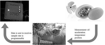
The experimental monitoring system was supplied by MKW Electronics in Weibern, Austria. It was tested from May 2012 to November 2013. The system consisted of ear tags, receivers and computing infrastructure to record data (Figure 1). It was equipped with 12 receivers, 10 mounted on the walls and two in the central area at about 2 m height, to capture the ear tags’ signals. The ear tags were fitted to the central inner surface of the sows’ ears. They sent data autonomously and unidirectionally to any of the receivers for pick-up.
Monitoring system. Sow with ear tag (middle), an ear tag (right) and a receiver (left).

The ear tags (each 34 g and 52×36×17 mm) were equipped with an accelerometer, a positioning system and two temperature sensors. One of the sensors was facing the sow’s ear and the other on the opposite surface. The present study focussed on the accelerometer data. The data from such an accelerometer consist of (x t , y t , z t )-triples of acceleration values measured along three internal axes at time t. Note that an ear tag is a very flexible way of mounting an acceleration sensor, and there was no approximately fixed reference plane relative to the ground plane, when a sow was standing upright. Furthermore, the ear tags were not rigidly fixated against the ear and could rotate with their spandrel. This suggested that using the three dimensions separately would introduce uncertainty about any sensor’s current orientation, which seemed hardly tractable for low sample rates.
The sample rate of such an accelerometer is programmable. Because of the trade-off between battery life and data resolution – a higher sample rate shortens battery life – the sample rate was set to 1 Hz, as battery life was perceived to be a limiting factor.
Data
A complete signal for a day and sow/ear tag consists of 3 axes×86 400 seconds×sample rate values together with their time stamps and the sow number. From the three-dimensional output (x t , y t , z t ) of acceleration values at time t, the series of total acceleration a t was then calculated as the Euclidean length:
 $$a_{t} \ {\equals}\ \sqrt {x_{t}^{2} \ {\plus}\ y_{t}^{2} \ {\plus}\ z_{t}^{2} } $$
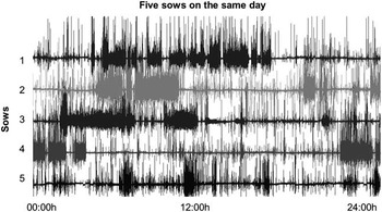
This results in a time series representing the distribution of total acceleration. As the accelerometers constantly measure the earth’s gravitational pull, the time series had a mean corresponding to that value. The mean was subtracted so that the remaining acceleration was genuinely generated by the activity of animals. Figure 2 shows typical total acceleration data for five different healthy sows on the same day. High activity corresponds to large deviations from the mean and low values to rest phases. The sows exhibit quite different behavioural or activity patterns as seen by different distributions of activity over a day.
Day-wise stacked acceleration signals for five different healthy sows recorded on the same day.

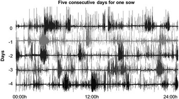
A visual inspection of the data from consecutive days for a single sow, illustrated in Figure 3, often does not reveal an apparent behavioural pattern, and the distribution of acceleration can differ between days.
Day-wise stacked acceleration signals from 5 consecutively recorded days for a single healthy sow.

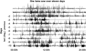
For some of the lame sows, on the other hand, a deviation from a seemingly persistent pattern of movement during a specific time of the day can be observed as early as 3 days before lameness diagnosis. An example of this is shown in Figure 4. On the last third of the days −10 to −4, an alternating pattern of phases of activity and resting time can be observed.
Example of a lame sow recorded over 11 days. The day of lameness diagnosis can be seen on top. Poor sampling quality is displayed by flat sections in the time series.

These bursts of activity are not present in the last three days towards lameness diagnosis. It also illustrates substantial data loss; straight-looking sections come from missing data. The data of this sow was therefore not used. The data quality in general, with the system being experimental, was rather poor. As seen, large patches of data were missing, and irregularly sampled time periods with only about 50% of the data available were found.
A data set was prepared for a numerical experiment to determine the basic feasibility of lameness detection from acceleration data using the method presented below. The data set consisted of acceleration data from the seven, best-sampled, lameness diagnosed sows, collected over a continuous period of 14 days, ending with the day of lameness diagnosis. Seven healthy sows were chosen for comparison, matched for time frame and with similar number of parities (2 to 5). Emphasis was placed on the sampling quality of individual time series, as the goal was to detect individual lameness. The 14-day spanning records were therefore chosen to be as complete and uninterrupted as possible with a mean of about 70 000 valid samples per day for both the lame and the healthy groups of the data set. This was well above the mean of all the data collected, which only had about 52 000 valid samples per day. There was no readily identifiable pattern for the data loss; it occurred randomly throughout.
The raw data of total acceleration was put in a ‘real-time’ format, whereby missing values were imputed with a mean value of 0. The missing data positions were stored in a separate indicator vector of missing or invalid values.
The developed method was to be applied to this sample to determine whether a lameness signal was at least detectable in the vicinity of a lameness diagnosis given immediate previous data.
Signal representation and feature calculation
A discrete wavelet transform was applied to each of the sows’ time series of total acceleration. A fairly comprehensive treatise on the foundations of wavelet theory was found by Mallat (Reference Mallat2008). The db4 wavelet and a decomposition level of 6 were chosen, so that the essential support of the wavelet kernel was about 4 s at the finest scale and about 4 min (~4×26 s) at the coarsest scale. The indicator vectors of missing and present values were disturbed with small random noise and simultaneously transformed. From a coefficient-wise comparison of these two latter transforms, it was decided whether a wavelet coefficient of the original acceleration time series was dominated by missing or present (valid) values. A coefficient was invalidated (set to zero, position stored) when it was dominated by missing values.
The obtained scales or time–frequency representation of wavelet coefficients as well as the original time series were then analysed separately. To that end, a collection of feature functions was applied locally over a short moving window. In principle, any function f of the data/signal s is admissible as a feature function. There are several well-known standard functions that may serve as feature functions. In the present study, local estimates of the energy (mean or sums of squares), energy of the derivative (2-variation) and variance were used. The local estimation was calculated for a short 360-sample-long window. This corresponds to 5 min of the original time series and a third of a day (~360×26) on the coarsest wavelet scale. Such an estimate was considered invalid, when the window contained less than 40% of valid samples. This resulted in three further feature series for each signal and its respective wavelet scales.
These feature series were then decomposed into level sets L i . A level set is a set of points in the domain of a time series s, where the values are in some defined range [l i −h,l i +h] called the level band:
 $$L_{i} \ {\equals}\ s^{{{\minus}1}} \left( {\left[ { l_{i} \ {\minus}\ h, l_{i} \ {\plus}\ h} \right]} \right)$$
Decomposition into five levels was undertaken for each of the feature series. The levels were computed in such a way that the level bands were occupied uniformly. The level-decomposition matrices thus consisted of five rows of logical vectors, with 1 indicating to which level the corresponding point belongs and 0 otherwise. From the decomposition into uniform levels, the expectation for each level could be known exactly: 1/number of levels. Therefore, invalid (i.e. missing) values could be imputed neutrally without changing the overall expectation and without introducing a spurious trend. The indicator vectors were then smoothed over a 24-h window to obtain a continuous density of level occupation. These level densities were then used to detect a change in sow behavioural pattern, indicating a potential lameness.
Detection method for lameness
The general strategy to implement lameness detection was based on the following reasoning: detecting lameness from acceleration time series first and foremost means monitoring a time series for changes within itself.
Therefore, the continuously recorded acceleration data and the derived feature series, s for brevity, of each animal were to be split into a past record of acceleration data s ref and a current (detection) part s det. The record in s ref was to serve as a reference for the animal’s usual and expected behavioural pattern. For the lame group, s ref should in all probability be less lameness impaired when compared with s det. For lameness detection, s det should be substantially differentiable from s ref. As acceleration time series are inherently noisy, a change in their properties should be better observable or measurable through a collection of feature series as constructed above.
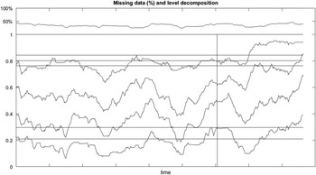
In concrete terms, following this general strategy, the level bands of highest and lowest values of each feature series were observed or monitored. It is to be expected that under a lameness condition, or even any impairment of physical health, the distribution of a feature series shifts towards fewer of high and more of low values. Therefore, a lameness condition should be detectable by the evolution of the lowest and highest bands towards unprecedented values in s det relative to the past reference record s ref. The last 3 days were taken as the detection phase, and all the previous days were declared as reference s ref. For each of the days in s ref, it was determined whether the 24-h-smooth density exceeded the corresponding extremal values from the reference phase. The density of the lowest level set was examined for an unprecedented maximum, whereas the highest level set was examined for an unprecedented minimum. If a previous extremum from the reference phase was breached, the feature was considered to be activated. The activation value was calculated as the integral over the breach in units of standard deviations as defined from the reference phase. Note that, by construction, none of the days from the reference period could possibly be detected as in breach. Figure 5 illustrates a level decomposition in accumulated form (cumulative sum of level densities). The vertical line separates the reference phase from the detection phase. The uppermost line is a 24-h-smooth of the data loss. Beneath the uppermost line is the density for the highest-value level, which appears mirrored from the accumulation. This in turn means looking for unprecedented maximal values for both the lowest and the highest level. The three straight lines about the highest level are its expectation for the reference phase, the expectation plus one standard deviation and the prediction phases’ maximum. It can be seen that the level density evolves outside the previously established range and breaches the maximum line for the last 2 days.
Cumulated level densities for the feature local energy on the second wavelet scale with the density of missing values on top. Reference and prediction phases are separated by the vertical line. For the highest band, the expectation, one standard deviation and the extremum from the reference phase are drawn as straight horizontal lines. The lowest band shows the standard deviation and the extremal lines.

The feature activations were then summed for each sow and each day from the detection phase, and a simple threshold classifier was applied to classify on the basis of the size of the breaches in the detection phase.
To introduce the metrics used to access the binary classifiers’ performance, let N and P denote the amount of negative (non-lame) and positive (lame) cases, respectively. The correctly classified cases are then called true negatives/positives and they (or their amounts) are denoted by TN and TP, whereas FN and FP stand for the (amount of the) incorrectly classified cases, which are called false negatives/positives.
The false-positive rate is then defined as FPR=FP/N, and the true negative rate, also called the specificity, is defined as TNR=TN/N(=1−FPR). The sensitivity of a classifier, also termed true-positive rate, is given by TPR=TP/P, whereas the accuracy ACC=(TP+TN/(P+N)) serves as an overall quality assessment involving both classes simultaneously.
Results
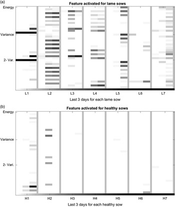
The calculated distributions of features activated over the original signals and the wavelet scales can be seen in the graphical representation (Figure 6) of the features activated per individual animal, day and feature function.
Individual feature activations for the lame sows (a) and the healthy sows (b). From left to right, the 7 triplets of days constituting the detection phase are shown, separated by thin, grey lines. From top to bottom (highest and lowest bands are alternating), energy, variation and variance feature activation are shown. The last row is the common scale.

Considerably more features were found in the state feature activated for the lame group than for the healthy sows. Although the feature value of an original signal can be in the state off, the distribution of that signal over the wavelet scales can produce several values in the state activated. Note that these are not statistically independent occurrences: when the percentage of some features changes in one of the scales, the percentage of said feature is bound to change on some (at least one) other scale as well.
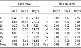
The accumulated day-wise feature activations (Table 1) for the detection phase overall had a mean of 8.8 for the lame group and 0.8 for the healthy group, and were thus clearly separable on a group level. From the day-wise means, the last day and the previous day were clearly separable from any of the healthy days. In general, for an individual classification, it is certainly necessary to confirm a given a priori grouping information in some separating statistic, but it might not be sufficient for a classification of individuals.
Sum of the individual feature activations per day for the lame (L1–L7, left side) and healthy sows (H1–H7, right side)

In bold are true-positive classifications obtained from a threshold that avoids false positives completely. (Day 0 is the day of diagnosis of the sows in the lame group.)
A strict threshold could be chosen to strictly exclude any false positives and subsequently determine how the sum of feature activated enables classification of individuals from the lame group. Consequently, the false-positive rate, FPR, was 0, and the specificity or true-negative rate, TNR=1−FPR, was 1. It was possible to classify 6 of the 7 lame sows as lame on at least one of the last 2 days. The true positives for the strict threshold are in bold in Table 1. The classifier statistics in Table 2 were calculated with the negative cases from the respective day solely as to not give an overly optimistic assessment of classifier performance. Using all available negative cases, although defendable, would of course elevate both ACC and TNR.
Classifier performance statistics

FPR=false-positive rate; TNR=true-negative rate; TPR=true-positive rate; ACC=accuracy for the last 3 days. The strict threshold avoids false positives completely, and the lax threshold optimises for accuracy.
A second, lax, threshold that allowed for false positives and maximised ACC was also applied. The TPR increases towards the last day for both thresholds, as does overall accuracy. The second last day was, with the exception of one sow, hardly if at all separable from the typical values found for the healthy sows.
Discussion
Relation to other methods
The ear is, from an acceleration measurement standpoint, perhaps the physically most decoupled body part of the locomotor system. The flexible mounting will, on the one hand, dampen the acceleration generated by locomotion; however, on the other hand, about any movement of the ear will show up as acceleration. Therefore, it seems not at all obvious that acceleration measurements from the ear should provide a specific assessment of lameness-related change in an animal’s activity pattern. Indeed, a direct effect of lameness would be an animal’s attempt to shift weight away from the affected leg, and thus force-measuring plates would be a way to detect anomaly in the weight distribution between legs. In a study by Pluym et al. (Reference Pluym, Maes, Vangeyte, Mertens, Baert, van Weyenberg, Millet and van Nuffel2013), a mobile walk-through construction with force plates did find a lameness effect in the weight distribution, but it is not clear whether it would be powerful enough to classify individually and whether the system would integrate seamlessly into operations.
Nonetheless, using ear tags to obtain acceleration or positioning data for lameness detection is an attractive proposition for the following reasons. First, ear tags are customary in animal farming. Second, the acceleration measurement within the ear tag is precise and basically lossless. The observed data loss seemingly occurred from corruption of the transmission from ear tag to receiver, which was addressed in later versions of the system. In principle, however, lameness information seems to be easily extractable from high-level features that are derived from positioning data such as estimating the distance covered per day through positional changes, termed ‘path length per day’. This held true in the study by Traulsen et al. (Reference Traulsen, Breitenberger, Auer, Stamer, Müller and Krieter2016), where, at least in the statistical sense, a mixed model found a significant effect up to 3 days before lameness. In contrast, the results for one simple acceleration-derived feature (variance) were negative. Although path length seems more direct or natural as it seemingly corresponds to well-known behavioural alterations such as ‘laying down more frequently’ (Gregoire et al., Reference Grégoire, Bergeron, D’Allaire, Meunier-Salaün and Devillers2013), the positioning system has clear drawbacks. It has a higher energy requirement and adds complexity to the system as it has to rely on real-time triangulation procedures for every single datum sampled. In contrast, acceleration data could be buffered in the ear tag until a complete transmission can be negotiated, and thus resolving data quality issues.
Data quality and classifier performance
Data quality was of major concern in the present study. The purpose of using a statistical model that looks for significant differences of some feature functions’ values between lame days and a non-lame past record would mainly be to determine whether that feature function is a good candidate for use in individual detection. To select feature functions this way, one may hope that data corruption evens itself out over a large data set. In contrast, monitoring individual time series to detect change will mainly rest on hindcasting a deviation from an individual past record. It ultimately means looking for a breakdown in a previously established self-similarity in some appropriate metric and is in all likelihood heavily dependent on the quality of the record. Therefore, the working sample was to have at least acceptable sampling quality. The data set selected still had a substantial data loss (about 20% per day on average), but was of better quality when compared with the total data (about 40% loss). It has to be remarked, however, that newer versions of the MKW-system deliver acceptable data quality with a typical data loss of about 10%. The quality requirements resulted in a small sample size of seven lame sows, which were matched with equally well-sampled healthy sows. It was the best sample to be obtained from the 196 sows that were fitted with ear tags. As a result, both the feature calculation and the subsequently applied classifier had to be kept as simple and robust as possible. The feature series calculation and level decomposition did not rely on any sample specifics – the robustness stems from the controllability of the level sets’ known expectation values. The extremal breach condition was from the first principled argument that the lowest energy band should rise, whereas the highest should diminish in density. The detection through a breach of previously established extremal values therefore is a very simple and robust proposition as it is also insusceptible to high activity/energy events such as heat occurrences in the reference phase. It would be easily possible to replace the extremal breach condition by a more relaxed one of the form w×σ (parameter×standard deviation). However, such parameters should be optimised and tested on a larger sample.
Likewise, the discrimination method ‘sum of feature activated’ depended on one single threshold, and therefore constituted a very simple classifier with a one-dimensional parameter space only. Here again, the sum of feature activated could be easily evaluated per feature class to provide more dimensions to work within classification. A more sophisticated classifier such as a support vector machine (Miekley et al., Reference Miekley, Traulsen and Krieter2013) might be able to discriminate with greater reliability (or margin), but this should be supported by a larger data set to train and test it properly.
A sample rate of 1 Hz, as used in this study, is obviously too low to resolve a signal into physically concise descriptions of motion patterns, as is argued by Robert et al. (Reference Robert, White, Renter and Larson2009). Whether or not the resolution is sufficient for that purpose, it is certainly possible to obtain statistics and extract features concerning patterns of movement or activity from these acceleration signals; the wavelet transform then can be seen as a mechanism to systematically and completely sample some abstract and uncorrelated (the summands from the decomposition are orthogonal) features from a signal. It would be interesting to see what type of information can be extracted by higher sampling rates of 5 or 10 Hz. Accelerometers in modern mobile phones, for example, can be used as a data source for a pedometer and high-level activity classification, but they typically sample at 30 to 60 Hz.
Although the last and previous days for the lame group are clearly distinguishable, the method should be further developed towards a longer lead or warning time. This might partly be achieved by considering longer time frames than 14 days. For a healthy case, the likelihood of extremal values falling into the prediction phase is then reduced. In case of a gradually progressing lameness, a longer record might be used to enhance the contrast between the reference and the prediction phase by introducing a censored part in the middle.
Improvement of methods
In order to improve the method towards greater margin of separability (between lame and healthy groups), a longer lead time and improved certainty, several aspects need to be improved upon. These are most crucially a more sophisticated, finer resolved feature representation and a more detailed understanding of healthy sows’ data.
In addressing a more finely resolved feature representation, note that feature calculation in 24-h windows only seemed advisable, as a day is a naturally cyclic unit of time, and a deviation from somewhat periodic patterns of behaviour is looked for. It is also a very coarse unit of time, and important information on the distribution of acceleration over a day is lost. Using smaller windows, for example, reveals these intra-day structures, but requires a more complex model for deviation detection. In particular, measures of autocorrelation could be used to capture change in finer patterns and serve to augment the feature representation.
From the mentioned alteration in behaviour by Gregoire et al. (Reference Grégoire, Bergeron, D’Allaire, Meunier-Salaün and Devillers2013), another way of augmenting the feature representation is suggestive: the inclusion of statistics derived from an activity classification (lying, walking, rooting) as high-level features. This would be (a pattern of) the time spent by the animal on a particular activity. It is unclear whether the classification results from, for example, Cornou et al. (Reference Cornou and Lundbye-Christensen2011), can be used to this end. In that study, all three dimensions from a neck-mounted sensor were utilised. Laying down time (low activity) was discriminated against moderate and high activity, but a higher sampling rate of 4 Hz was used, and the neck-mounted sensors could be gauged for upright standing/position.
The reason for aiming at a better understanding of healthy sows’ data is that lame samples are scarce, and it might not be sufficient to rely on lame samples solely as supervision. In order to make good use of the numerous healthy sows’ data, a machine might be trained to recognise a feature representation of healthy sows’ data exclusively by way of compressing or sparsely encoding it. This would effectively result in a more adapted, higher-level feature representation. As a refined prediction method, it would then look for a higher reconstruction error in lame sows’ data than on unseen healthy samples, that is, samples not used for training the encoder. For such more refined purposes, data quality is crucial, as a more localised calculation of features or activity classification will have to rely on relatively complete data.
Conclusion
A representation of acceleration data based on wavelet-derived feature series and level decompositions was developed, fit for the application of an ‘extremal’ model for deviation detection as lameness detector. In view of the poor data quality and small sample size, it could be kept robust against data loss and does not rely on parameters that could possibly overfit the small sample. Our results indicate that the described method may be feasible for implementing lameness detection. However, it should of course be tested on a larger sample. Improvements should be obtainable by localising time and evaluating the resulting patterns.
Acknowledgements
This Project has been supported by the Bundesministerium für Ernährung und Landwirtschaft [Federal Ministry of Food and Agriculture] (BMEL).