2 Gaussian filtering and linearity

We begin by considering the case of an infinitely long (two-dimensional (2-D)) lifting surface. In that case, the lift force (per unit fluid mass) as an actuator line may be thought of as distributed over a (singular) line, according to:

(2.1) $$\begin{eqnarray}\frac{1}{\unicode[STIX]{x1D70C}}f_{y}(x,y,z)=-\unicode[STIX]{x1D6E4}U_{\infty }\unicode[STIX]{x1D6FF}(x)\unicode[STIX]{x1D6FF}(y)=-\frac{1}{2}c_{L}cU_{\infty }^{2}\unicode[STIX]{x1D6FF}(x)\unicode[STIX]{x1D6FF}(y).\end{eqnarray}$$

Here, $\unicode[STIX]{x1D6E4}$ is the circulation, $U_{\infty }$ the inflow velocity, $c$ the chord length, $c_{L}$ the lift coefficient and $\unicode[STIX]{x1D6FF}$ are delta Dirac functions. Also, $x$ is the coordinate in the direction of the incoming flow, $y$ is the direction of the lift force and $z$ is the coordinate along the blade span. We consider the actuator line model using a (three-dimensional (3-D)) Gaussian kernel as proposed in the original introduction of the ALM (Sørensen & Shen Reference Sørensen and Shen2002):

(2.2) $$\begin{eqnarray}\unicode[STIX]{x1D702}_{\unicode[STIX]{x1D716}}(x,y,z)=\frac{1}{\unicode[STIX]{x1D716}^{3}\unicode[STIX]{x03C0}^{3/2}}\text{e}^{-(x^{2}+y^{2}+z^{2})/\unicode[STIX]{x1D716}^{2}}.\end{eqnarray}$$

For the case of an infinitely long blade, integration along the spanwise direction (from $z=-\infty$ to $z=\infty$ ) leads to the 2-D force distribution:

(2.3) $$\begin{eqnarray}\frac{1}{\unicode[STIX]{x1D70C}}\widetilde{f}_{y}(\boldsymbol{x})=\int \frac{1}{\unicode[STIX]{x1D70C}}f_{y}(\boldsymbol{x}^{\prime })\unicode[STIX]{x1D702}_{\unicode[STIX]{x1D716}}(\boldsymbol{x}-\boldsymbol{x}^{\prime })d^{3}\boldsymbol{x}^{\prime }=-\frac{1}{\unicode[STIX]{x1D716}^{2}\unicode[STIX]{x03C0}}\frac{1}{2}c_{L}cU_{\infty }^{2}\text{e}^{-(x^{2}+y^{2})/\unicode[STIX]{x1D716}^{2}}.\end{eqnarray}$$

As derived in Martínez-Tossas et al. (Reference Martínez-Tossas, Churchfield and Meneveau2017), the curl of this force is a source in the transport equation for the $z$ -component vorticity. The linearized $z$ -component vorticity transport equation (linearized in the sense that the advection velocity in the $x$ -direction is set to a constant velocity $U_{\infty }$ everywhere) was integrated and the $z$ -component vorticity distribution derived. The result is a Gaussian distribution with width $\unicode[STIX]{x1D716}$ (see also Forsythe et al. Reference Forsythe, Lynch, Polsky and Spalart2015). Applying Biot–Savart then leads to the perturbation (tangential) velocity distribution:

(2.4) $$\begin{eqnarray}\widetilde{u}_{\unicode[STIX]{x1D703}}^{\prime }=\frac{1}{4\unicode[STIX]{x1D70B}}c_{L}U_{\infty }\frac{c}{r}(1-\text{e}^{-r^{2}/\unicode[STIX]{x1D716}^{2}}),\end{eqnarray}$$

where $r^{2}=x^{2}+y^{2}$ . This flow is a Lamb–Oseen vortex with core size $\unicode[STIX]{x1D716}$ representing the bound vorticity resulting from the Gaussian-filtered lifting surface.

It turns out that the same result is obtained if one simply applies the Gaussian filter to an ideal vortex velocity distribution. That is to say, recall that if one uses Biot–Savart on the initially unfiltered line vortex, one obtains the ideal bound vortex with tangential perturbation velocity $u_{\unicode[STIX]{x1D703}}^{\prime }=(1/4\unicode[STIX]{x1D70B})c_{L}U_{\infty }(c/r)$ . When this velocity is filtered (in two dimensions) using the kernel $\unicode[STIX]{x1D702}_{\unicode[STIX]{x1D716}}(x,y)$ , the same Lamb–Oseen vortex with tangential velocity $\tilde{u} _{\unicode[STIX]{x1D703}}^{\prime }$ and core size $\unicode[STIX]{x1D716}$ as given in (2.4) is obtained. This equivalence occurs because the relationship between perturbation velocity and applied force, under the assumption of linearized perturbation vorticity transport, is linear. That is to say, we can write $\boldsymbol{u}^{\prime }={\mathcal{L}}(\,\boldsymbol{f})$ , where ${\mathcal{L}}$ represents linear operations (taking the curl of the force, integrating the linearized vorticity transport equation and applying Biot–Savart). Applying the Gaussian filter to this expression leads to $\widetilde{\boldsymbol{u}}^{\prime }=\widetilde{{\mathcal{L}}(\,\boldsymbol{f})}={\mathcal{L}}(\,\widetilde{\boldsymbol{f}})$ , allowing us to obtain the result of Martínez-Tossas et al. (Reference Martínez-Tossas, Churchfield and Meneveau2017) by simply filtering the ideal vortex tangential velocity distribution.

Next, we consider the case of a finite-length lifting surface represented as a singular line as in (2.1) but with $\unicode[STIX]{x1D6E4}(z)=0$ for $z<0$ . Figure 1(a) shows the coordinate system for which $z=0$ is at the tip of the blade and the blade extends toward $z>0$ .

Figure 1.

(a) Sketch of finite lifting surface, where the origin of the coordinate system is placed at the blade tip, where $z=0$ . (b) Illustration of the Gaussian-filtered actuator line model with a force distribution across the blade’s cross-section and $z$ -dependent lift force (or circulation) distribution. Also shown (in green) are some ‘thick’ shed vortices and (in blue along the $z$ -axis) their induced velocity, $u_{y}^{\prime }$ . The distribution of the total induced $y$ -velocity as a function of the span is obtained by an integration over induced velocity from the shed vorticity.

In this case, classical lifting line theory states that because $\unicode[STIX]{x1D6E4}$ in (2.1) depends on  $z$ , vorticity is shed, generating an induced velocity at the blade that changes the angle of attack and affects the lift coefficient and thus $\unicode[STIX]{x1D6E4}$ itself. A self-consistency condition leads to the classical integro-differential equation for the circulation (Prandtl & Tietjens Reference Prandtl and Tietjens1957) along the blade:

(2.5) $$\begin{eqnarray}\unicode[STIX]{x1D6E4}(z)=\frac{1}{2}\left(c_{Lb}+\frac{\text{d}c_{Lb}}{\text{d}\unicode[STIX]{x1D6FC}}\frac{u_{y}^{\prime }(z)}{U_{\infty }}\right)cU_{\infty }=\frac{1}{2}c_{Lb}cU_{\infty }+\frac{1}{2}\frac{\text{d}c_{Lb}}{\text{d}\unicode[STIX]{x1D6FC}}c\int _{0}^{L}\frac{\unicode[STIX]{x1D6E4}^{\prime }(z^{\prime })}{4\unicode[STIX]{x03C0}(z^{\prime }-z)}\,\text{d}z^{\prime },\end{eqnarray}$$

where $c_{Lb}$ is the lift coefficient at the baseline angle of attack (i.e. corresponding to the local free-stream velocity  $U_{\infty }$ ), $\text{d}c_{Lb}/\text{d}\unicode[STIX]{x1D6FC}$ is the slope of the lift versus angle of attack curve (typically close to $2\unicode[STIX]{x03C0}$ ) and $u_{y}^{\prime }(z)$ is the induced downwash velocity at position $z$ because of changes in circulation everywhere on the blade of span  $L$ . The typical approach solves this equation by expanding $\unicode[STIX]{x1D6E4}(z)$ into a Fourier series, and using the condition that $\unicode[STIX]{x1D6E4}(z)=0$ at the blade tips leads to the choice of a sine series. In general, the Fourier coefficients must be found numerically, even for the simple case of a constant chord and baseline lift parameters, $c_{Lb}$ and $\text{d}c_{Lb}/\text{d}\unicode[STIX]{x1D6FC}$ . Stewartson (Reference Stewartson1960) provides an analytical solution for the case of a semi-infinite constant chord wing.

At this stage, consider the case when the corresponding lift force distribution

(2.6) $$\begin{eqnarray}\displaystyle \frac{1}{\unicode[STIX]{x1D70C}}f_{y}(x,y,z) & = & \displaystyle -\unicode[STIX]{x1D6E4}(z)U_{\infty }\unicode[STIX]{x1D6FF}(x)\unicode[STIX]{x1D6FF}(y)H(z)\nonumber\\ \displaystyle & = & \displaystyle -\frac{1}{2}\left(c_{Lb}+\frac{\text{d}c_{Lb}}{\text{d}\unicode[STIX]{x1D6FC}}\frac{u_{y}^{\prime }(x,y,z)}{U_{\infty }}\right)cU_{\infty }^{2}\unicode[STIX]{x1D6FF}(x)\unicode[STIX]{x1D6FF}(y)H(z),\end{eqnarray}$$

is filtered with the Gaussian kernel, $\unicode[STIX]{x1D702}_{\unicode[STIX]{x1D716}}$ ( $H(z)$ is the Heaviside function because there is no force at $z<0$ even if $u_{y}^{\prime }$ is non-zero there). Even though in this case we can still write a linear equation, $\boldsymbol{u}^{\prime }={\mathcal{L}}(\,\boldsymbol{f})={\mathcal{L}}(\,\boldsymbol{f}_{b}+c_{1}\boldsymbol{u}^{\prime })$ , the spatially filtered velocity no longer solves the same equation as the original lifting line theory:

(2.7) $$\begin{eqnarray}\widetilde{\boldsymbol{u}}^{\prime }={\mathcal{L}}(\,\widetilde{\boldsymbol{f}})={\mathcal{L}}(\,\widetilde{\boldsymbol{f}}_{b}+\widetilde{c_{1}\boldsymbol{u}^{\prime }})\neq {\mathcal{L}}(\tilde{\boldsymbol{f}}_{b}+c_{1}\widetilde{\boldsymbol{u}}^{\prime }).\end{eqnarray}$$

The reason is that the prefactor, $c_{1}$ , in this case contains the Heaviside function, $H(z)$ , and clearly $\widetilde{H\boldsymbol{u}_{y}^{\prime }}\neq H\widetilde{\boldsymbol{u}^{\prime }}_{y}$ . Further, the velocity field induced by a force filtered at scale $\unicode[STIX]{x1D716}$ is given by:

(2.8) $$\begin{eqnarray}\boldsymbol{u}_{\unicode[STIX]{x1D716}}^{\prime }={\mathcal{L}}(\,\widetilde{\boldsymbol{f}})={\mathcal{L}}(\,\widetilde{\boldsymbol{f}}_{b}+\widetilde{c_{1}\boldsymbol{u}_{\unicode[STIX]{x1D716}}^{\prime }}).\end{eqnarray}$$

Clearly, ${\boldsymbol{u}^{\prime }}_{\unicode[STIX]{x1D716}}\neq \widetilde{\boldsymbol{u}^{\prime }}$ because $\widetilde{c_{1}\boldsymbol{u}^{\prime }}\neq \widetilde{c_{1}\widetilde{\boldsymbol{u}}^{\prime }}$ . As a result, we cannot simply use the solution of the classical lifting line theory, $\boldsymbol{u}^{\prime }$ , for an ideal line force and spatially filter the velocity to obtain the correct result corresponding to a filtered force distribution along a finite-length lifting blade. A full derivation is therefore needed to determine $\boldsymbol{u}_{\unicode[STIX]{x1D716}}^{\prime }$ as solution to (2.8), to which the next section is devoted.

3 Gaussian-filtered lifting line theory

For generality, we assume a span-dependent chord length, $c(z)$ , inflow velocity, $U_{\infty }(z)$ and lift coefficient, $c_{L}(z;\unicode[STIX]{x1D716})$ and we note that the effective lift coefficient depends upon the kernel size, $\unicode[STIX]{x1D716}(z)$ . We define $c_{Lb}(z)$ to be the (known) lift coefficient at the baseline angle of attack (i.e. corresponding to the local free-stream velocity, $U_{\infty }(z)$ ). For simplicity, we assume that the chord and kernel size do not vary rapidly along the span (i.e. at various stages we will assume $\text{d}c/\text{d}z\ll 1$ and $\text{d}\unicode[STIX]{x1D716}/\text{d}z\ll 1$ ). Later, applications with variable $\unicode[STIX]{x1D716}(z)$ and $c(z)$ will show that accurate results may also be obtained in such cases.

As in the prior section, we consider the unfiltered actuator line to be a lifting surface represented as a ‘delta function’ distribution in the $xy$ plane and a $z$ -dependent force (per unit length) along a line (i.e. the $z$ -dependent lift distribution) is given by:

(3.1) $$\begin{eqnarray}\frac{1}{\unicode[STIX]{x1D70C}}f_{y}(x,y,z)=-G(z)\unicode[STIX]{x1D6FF}(x)\unicode[STIX]{x1D6FF}(y),\end{eqnarray}$$

where

(3.2) $$\begin{eqnarray}G(z)=\unicode[STIX]{x1D6E4}(z)U_{\infty }(z)={\textstyle \frac{1}{2}}c_{L}(z)c(z)U_{\infty }^{2}(z)H(z).\end{eqnarray}$$

To explicitly take into account modifications of the local lift coefficient due to changes in incident velocity direction, we recall that the effective lift coefficient can be written as:

(3.3) $$\begin{eqnarray}c_{L}(z;\unicode[STIX]{x1D716})=c_{Lb}(z)+\frac{\text{d}c_{L}}{\text{d}\unicode[STIX]{x1D6FC}}(z)\frac{u_{y}^{\prime }(0,0,z;\unicode[STIX]{x1D716})}{U_{\infty }(z)},\end{eqnarray}$$

where $u_{y}^{\prime }(0,0,z;\unicode[STIX]{x1D716})$ is the local perturbation velocity (evaluated at $x=y=0$ ) due to downwash from shed vorticity. For an ideal lifting surface, one may use $\text{d}c_{L}/\text{d}\unicode[STIX]{x1D6FC}=2\unicode[STIX]{x03C0}$ but, in practice, different values may be used.

As described in the preceding section, in the actuator line model the actual force per unit volume seen by the fluid is given by the convolution of the line strength with the Gaussian kernel $\unicode[STIX]{x1D702}_{\unicode[STIX]{x1D716}}$ according to:

(3.4) $$\begin{eqnarray}\displaystyle \frac{1}{\unicode[STIX]{x1D70C}}\widetilde{f}_{y}(\boldsymbol{x}) & = & \displaystyle \int \frac{1}{\unicode[STIX]{x1D70C}}f_{y}(\boldsymbol{x}^{\prime })\unicode[STIX]{x1D702}_{\unicode[STIX]{x1D716}}(\boldsymbol{x}-\boldsymbol{x}^{\prime })\,\text{d}^{3}\boldsymbol{x}^{\prime }\nonumber\\ \displaystyle & = & \displaystyle -\iiint \frac{1}{\unicode[STIX]{x1D716}^{3}\unicode[STIX]{x03C0}^{3/2}}G(z^{\prime })\unicode[STIX]{x1D6FF}(x^{\prime })\unicode[STIX]{x1D6FF}(y^{\prime })\text{e}^{-[(x-x^{\prime })^{2}+(y-y^{\prime })^{2}+(z-z^{\prime })^{2}]/\unicode[STIX]{x1D716}^{2}}\,\text{d}x^{\prime }\,\text{d}y^{\prime }\,\text{d}z^{\prime }.\quad\end{eqnarray}$$

Evaluating the $xy$ integrals and changing variables to $z^{\prime \prime }=z^{\prime }-z$ , we obtain:

(3.5) $$\begin{eqnarray}\frac{1}{\unicode[STIX]{x1D70C}}\widetilde{f}_{y}(x,y,z)=\frac{1}{\unicode[STIX]{x1D70C}}f_{y}(x,y,z;\unicode[STIX]{x1D716})=-\frac{1}{\unicode[STIX]{x1D716}^{3}\unicode[STIX]{x03C0}^{3/2}}\text{e}^{-(x^{2}+y^{2})/\unicode[STIX]{x1D716}^{2}}\int _{-\infty }^{\infty }G(z^{\prime \prime }+z)\text{e}^{-z^{\prime \prime 2}/\unicode[STIX]{x1D716}^{2}}\,\text{d}z^{\prime \prime },\end{eqnarray}$$

where from here on we omit tildes to denote filtered variables and indicate their dependence on $\unicode[STIX]{x1D716}$ instead.

3.1 Distribution of shed vorticity

Next, we consider the steady-state vorticity transport equation for the streamwise vorticity component in the presence of the Gaussian-filtered lift body force in ideal, steady flow (neglecting viscosity and turbulence), also neglecting changes in advective velocity due to the vorticity (linearization). The only term generating vorticity is the curl of the Gaussian body force, whose streamwise component can be expressed in the $x$ -component vorticity transport equation:

(3.6) $$\begin{eqnarray}U_{\infty }(z)\frac{\unicode[STIX]{x2202}\unicode[STIX]{x1D714}_{x}}{\unicode[STIX]{x2202}x}=\frac{1}{\unicode[STIX]{x1D70C}}(\unicode[STIX]{x1D735}\times \boldsymbol{f})_{x}=-\frac{1}{\unicode[STIX]{x1D70C}}\frac{\unicode[STIX]{x2202}f_{y}}{\unicode[STIX]{x2202}z}=\frac{\text{e}^{-(x^{2}+y^{2})/\unicode[STIX]{x1D716}^{2}}}{\unicode[STIX]{x1D716}^{3}\unicode[STIX]{x03C0}^{3/2}}\int _{-\infty }^{\infty }\frac{\text{d}}{\text{d}z}G(z^{\prime \prime }+z)\text{e}^{-z^{\prime \prime 2}/\unicode[STIX]{x1D716}^{2}}\,\text{d}z^{\prime \prime }.\end{eqnarray}$$

Integrating in $x$ between $-\infty$ and $x$ , assuming that $\unicode[STIX]{x1D714}_{x}=0$ when $x\rightarrow -\infty$ and changing variables back to $z^{\prime }=z^{\prime \prime }+z$ , yields the following streamwise vorticity distribution:

(3.7) $$\begin{eqnarray}\unicode[STIX]{x1D714}_{x}(\boldsymbol{x};\unicode[STIX]{x1D716})=\frac{1}{2U_{\infty }(z)\unicode[STIX]{x1D716}^{2}\unicode[STIX]{x03C0}}[\text{erf}(x/\unicode[STIX]{x1D716})+1]\text{e}^{-y^{2}/\unicode[STIX]{x1D716}^{2}}\int _{-\infty }^{\infty }\frac{\text{d}G(z^{\prime })}{\text{d}z^{\prime }}\text{e}^{-(z-z^{\prime })^{2}/\unicode[STIX]{x1D716}^{2}}\,\text{d}z^{\prime }.\end{eqnarray}$$

This $\unicode[STIX]{x1D714}_{x}(\boldsymbol{x};\unicode[STIX]{x1D716})$ distribution arises from the downstream transport of the fluid rotation induced by the transverse variations of lift induced by the Gaussian-filtered ALM force. Approaching the blade near the tip with the free stream, the vorticity rises from zero to its downstream value following the error function, it has a Gaussian profile in the cross-stream $y$ -direction, while the shape of the tip vortex in the spanwise direction is non-trivial and involves the integrated effects from the possibly varying lift coefficient. If the actual lift coefficient, chord and velocity were constant for $z>0$ and zero otherwise (i.e. $G(z)=(1/2)c_{L0}cU_{\infty 0}^{2}H(z)$ so that $G^{\prime }(z)=(1/2)c_{L0}cU_{\infty 0}^{2}\unicode[STIX]{x1D6FF}(z)$ ) and if the lift did not change with angle of attack (i.e. $\text{d}c_{L}/\text{d}\unicode[STIX]{x1D6FC}=0$ , which is unphysical), equation (3.7) shows that the tip vortex for $x/\unicode[STIX]{x1D716}\gg 1$ is a Lamb–Oseen vortex with Gaussian vorticity distribution in the $zy$ plane whose core size is precisely $\unicode[STIX]{x1D716}$ (similar to the bound vortex representing the blade circulation in the $xy$ plane analysed in Martínez-Tossas et al. Reference Martínez-Tossas, Churchfield and Meneveau2017). However, the induced velocity changes the local lift coefficient and so we seek a more general solution that takes this effect into account.

3.2 Induced velocity perturbation

To find the induced vertical velocity along the blade associated with this 3-D vorticity distribution, we use the Biot–Savart equation:

(3.8) $$\begin{eqnarray}\left.\begin{array}{@{}c@{}}\displaystyle u_{y}^{\prime }(0,0,z;\unicode[STIX]{x1D716})=-\frac{1}{4\unicode[STIX]{x03C0}}\iiint \frac{\unicode[STIX]{x1D714}_{x}(\boldsymbol{x}^{\prime \prime };\unicode[STIX]{x1D716})(z-z^{\prime \prime })}{(x^{\prime \prime 2}+y^{\prime \prime 2}+(z-z^{\prime \prime })^{2})^{3/2}}\,\text{d}^{3}\boldsymbol{x}^{\prime \prime }=-\frac{1}{8\unicode[STIX]{x03C0}^{2}\unicode[STIX]{x1D716}^{2}}\int _{-\infty }^{\infty }\frac{\text{d}G(z^{\prime })}{\text{d}z^{\prime }}\\ \displaystyle \iiint \frac{1}{U_{\infty }(z^{\prime \prime })}\frac{(z-z^{\prime \prime })[\text{erf}(x^{\prime \prime }/\unicode[STIX]{x1D716})+1]}{[x^{\prime \prime 2}+y^{\prime \prime 2}+(z-z^{\prime \prime })^{2}]^{3/2}}\text{e}^{-(y^{\prime \prime 2}+(z^{\prime \prime }-z^{\prime })^{2})/\unicode[STIX]{x1D716}^{2}}\,\text{d}x^{\prime \prime }\,\text{d}y^{\prime \prime }\,\text{d}z^{\prime \prime }\,\text{d}z^{\prime }.\end{array}\right\}\end{eqnarray}$$

To proceed, it is useful to neglect the $z^{\prime \prime }$ variations of $U_{\infty }(z^{\prime \prime })$ in the denominator inside the integral and approximate $U_{\infty }(z^{\prime \prime })\approx U_{\infty }(z)$ . This can be justified because the kernel $(z-z^{\prime \prime })/|\boldsymbol{x}-\boldsymbol{x}^{\prime \prime }|^{3}$ peaks at $z^{\prime \prime }=z$ . Furthermore, we recognize that the integrand in $x^{\prime \prime }$ is even in the denominator while in the numerator the $\text{erf}(..)$ term is odd. Hence, we are left with:

(3.9) $$\begin{eqnarray}u_{y}^{\prime }(0,0,z;\unicode[STIX]{x1D716})=-\frac{1}{8\unicode[STIX]{x03C0}^{2}\unicode[STIX]{x1D716}^{2}U_{\infty }(z)}\int _{-\infty }^{\infty }\frac{\text{d}G(z^{\prime })}{\text{d}z^{\prime }}\iiint \frac{(z-z^{\prime \prime })\text{e}^{-(y^{\prime \prime 2}+(z^{\prime \prime }-z^{\prime })^{2})/\unicode[STIX]{x1D716}^{2}}}{[x^{\prime \prime 2}+y^{\prime \prime 2}+(z-z^{\prime \prime })^{2}]^{3/2}}\,\text{d}x^{\prime \prime }\,\text{d}y^{\prime \prime }\,\text{d}z^{\prime \prime }\,\text{d}z^{\prime },\end{eqnarray}$$

which, with an additional change of variables, $\unicode[STIX]{x1D701}=z^{\prime \prime }-z^{\prime }$ can be rewritten as:

(3.10) $$\begin{eqnarray}u_{y}^{\prime }(0,0,z;\unicode[STIX]{x1D716})=-\frac{1}{8\unicode[STIX]{x03C0}^{2}\unicode[STIX]{x1D716}U_{\infty }(z)}\int _{-\infty }^{\infty }\frac{\text{d}G(z^{\prime })}{\text{d}z^{\prime }}F(z-z^{\prime })\,\text{d}z^{\prime },\end{eqnarray}$$

where

(3.11) $$\begin{eqnarray}F(z)=\frac{1}{\unicode[STIX]{x1D716}}\iiint \frac{(z-\unicode[STIX]{x1D701})}{[x^{\prime \prime 2}+y^{\prime \prime 2}+(z-\unicode[STIX]{x1D701})^{2}]^{3/2}}\text{e}^{-(y^{\prime \prime 2}+\unicode[STIX]{x1D701}^{2})/\unicode[STIX]{x1D716}^{2}}\,\text{d}x^{\prime \prime }\,\text{d}y^{\prime \prime }\,\text{d}\unicode[STIX]{x1D701}.\end{eqnarray}$$

The integration yields (Martínez-Tossas Reference Martínez-Tossas2017):

(3.12) $$\begin{eqnarray}F(z)=\frac{2\unicode[STIX]{x03C0}\unicode[STIX]{x1D716}}{z}\left(1-\text{e}^{-(z/\unicode[STIX]{x1D716})^{2}}\right).\end{eqnarray}$$

Hence, we find that the velocity perturbation may be written as a superposition of shifted Lamb–Oseen vortices, weighted by the gradient of the lift function  $G(z)$ :

(3.13) $$\begin{eqnarray}u_{y}^{\prime }(z;\unicode[STIX]{x1D716})=-\frac{1}{U_{\infty }(z)}\int _{-\infty }^{\infty }\frac{\text{d}G(z^{\prime })}{\text{d}z^{\prime }}\frac{1}{4\unicode[STIX]{x03C0}(z-z^{\prime })}\left(1-\text{e}^{-(z-z^{\prime })^{2}/\unicode[STIX]{x1D716}^{2}}\right)\,\text{d}z^{\prime },\end{eqnarray}$$

where $u_{y}^{\prime }(0,0,z;\unicode[STIX]{x1D716})$ on the $x=y=0$ axis has been denoted as $u_{y}^{\prime }(z;\unicode[STIX]{x1D716})$ , also indicating that the solution depends on the kernel width, $\unicode[STIX]{x1D716}$ . This is the Gaussian force field analogue of lifting line theory in which the induced velocity from thin tip vortices may be expressed as an integral of the spanwise derivative of circulation. Because of the Gaussian smoothing, a Lamb–Oseen kernel arises in this expression, again with a core size exactly equal to $\unicode[STIX]{x1D716}$ used in the Gaussian applied body force that represents the lifting surface. Note that the same expression proposed by Dag (Reference Dag2017) and Dag & Sørensen (Reference Dag and Sørensen2018) was based on observations that smoothed tip vortices in ALM have the shape of Lamb–Oseen vortices. The result in (3.13) serves as formal proof that their empirically motivated approach can also be derived from first principles. It also enables further analysis and solution methods as detailed below.

Since the effective lift coefficient will vary due to the induced downwash, the strength of the vortex spanwise change, $\text{d}G(z^{\prime })/\text{d}z^{\prime }$ , will be affected by the downwash as a result of a modification of  $c_{L}(z)$ :

(3.14) $$\begin{eqnarray}\left.\begin{array}{@{}c@{}}\displaystyle G(z)=G_{b}(z)+\frac{1}{2}\frac{\text{d}c_{L}}{\text{d}\unicode[STIX]{x1D6FC}}(z)u_{y}^{\prime }(z;\unicode[STIX]{x1D716})U_{\infty }(z)c(z),\quad \text{where}\\ \displaystyle G_{b}(z)=\frac{1}{2}c_{Lb}(z)c(z)U_{\infty }^{2}(z)\end{array}\right\}\end{eqnarray}$$

corresponds to the ‘baseline’ case (i.e. the lift coefficient appropriate for the undisturbed inflow angle of attack) without downwash. Replacing $G(z)$ in (3.13), we obtain:

(3.15) $$\begin{eqnarray}\displaystyle u_{y}^{\prime }(z;\unicode[STIX]{x1D716})U_{\infty }(z) & = & \displaystyle \int _{-\infty }^{\infty }\frac{\text{d}G_{b}(z^{\prime })}{\text{d}z^{\prime }}g(z-z^{\prime };\unicode[STIX]{x1D716})\,\text{d}z^{\prime }\nonumber\\ \displaystyle & & \displaystyle +\,\int _{-\infty }^{\infty }\frac{\text{d}}{\text{d}z^{\prime }}\left[\frac{1}{2}\frac{\text{d}c_{L}}{\text{d}\unicode[STIX]{x1D6FC}}(z^{\prime })u_{y}^{\prime }(z^{\prime };\unicode[STIX]{x1D716})U_{\infty }(z^{\prime })c(z^{\prime })\right]g(z-z^{\prime };\unicode[STIX]{x1D716})\,\text{d}z^{\prime },\qquad\end{eqnarray}$$

where

(3.16) $$\begin{eqnarray}g(z,\unicode[STIX]{x1D716})=-\frac{1}{4\unicode[STIX]{x03C0}z}(1-\text{e}^{-z^{2}/\unicode[STIX]{x1D716}^{2}}).\end{eqnarray}$$

This expression is an integro-differential equation that also appears in the classical lifting line theory. In prior applications (without the Gaussian filtering), such an equation (usually formulated for the circulation) is solved for each case using a sine series expansion. Here, we propose to first recast this expression as a proper Fredholm integral equation of the second kind, using integration by parts for the second term:

(3.17) $$\begin{eqnarray}\displaystyle u_{y}^{\prime }(z;\unicode[STIX]{x1D716})U_{\infty }(z) & = & \displaystyle \int _{-\infty }^{\infty }\frac{\text{d}G_{b}(z^{\prime })}{\text{d}z^{\prime }}g(z-z^{\prime },\unicode[STIX]{x1D716})\,\text{d}z^{\prime }\nonumber\\ \displaystyle & & \displaystyle +\,\int _{-\infty }^{\infty }\unicode[STIX]{x1D703}(z^{\prime })u_{y}^{\prime }(z^{\prime };\unicode[STIX]{x1D716})U_{\infty }(z^{\prime })c(z^{\prime })k(z-z^{\prime };\unicode[STIX]{x1D716})\,\text{d}z^{\prime },\end{eqnarray}$$

where

(3.18) $$\begin{eqnarray}k(z;\unicode[STIX]{x1D716})=\unicode[STIX]{x03C0}\frac{\text{d}}{\text{d}z}\left[-\frac{1}{4\unicode[STIX]{x03C0}z}(1-\text{e}^{-z^{2}/\unicode[STIX]{x1D716}^{2}})\right]=\frac{1}{4z^{2}}(1-\text{e}^{-z^{2}/\unicode[STIX]{x1D716}^{2}})-\frac{1}{2\unicode[STIX]{x1D716}^{2}}\text{e}^{-z^{2}/\unicode[STIX]{x1D716}^{2}}.\end{eqnarray}$$

Note that we have also introduced a variable that describes possible deviations from the idealized lift curve slope:

(3.19) $$\begin{eqnarray}\unicode[STIX]{x1D703}(z)=\frac{1}{2\unicode[STIX]{x03C0}}\frac{\text{d}c_{L}}{\text{d}\unicode[STIX]{x1D6FC}}(z).\end{eqnarray}$$

The equation is cast most naturally in terms of the unknown perturbation momentum flux:

(3.20) $$\begin{eqnarray}M(z;\unicode[STIX]{x1D716})=u_{y}^{\prime }(z;\unicode[STIX]{x1D716})U_{\infty }(z)c(z).\end{eqnarray}$$

Multiplying (3.17) by $c(z)$ yields:

(3.21) $$\begin{eqnarray}M(z;\unicode[STIX]{x1D716})=\int _{-\infty }^{\infty }\frac{\text{d}G_{b}(z^{\prime })}{\text{d}z^{\prime }}c(z)g(z-z^{\prime };\unicode[STIX]{x1D716})\,\text{d}z^{\prime }+\int _{-\infty }^{\infty }\unicode[STIX]{x1D703}(z^{\prime })M(z^{\prime };\unicode[STIX]{x1D716})c(z)k(z-z^{\prime };\unicode[STIX]{x1D716})\,\text{d}z^{\prime }.\end{eqnarray}$$

For general distributions of $c(z)$ , $\unicode[STIX]{x1D716}(z)$ and $\unicode[STIX]{x1D703}(z)$ along the blade, one must solve this integral equation numerically for each individual case.

4 Simplifications, solutions and approximate analytical fit

Next, we propose an approximate method that will be shown to be of sufficient accuracy for many applications and helpful as a reference solution of an interesting special case. Specifically, we consider a lifting surface extending to lengths much larger than the chord length. The blade tip is located at, say, $z=0$ . Also, we approximate $\unicode[STIX]{x1D703}(z)$ by its average distribution over the blade, $\overline{\unicode[STIX]{x1D703}}$ (i.e. $\unicode[STIX]{x1D703}(z)\approx \overline{\unicode[STIX]{x1D703}}H(z)$ ). Under these conditions, we may rewrite (3.21) as:

(4.1) $$\begin{eqnarray}M(z;\unicode[STIX]{x1D716})=\int _{-\infty }^{\infty }\frac{\text{d}G_{b}(z^{\prime })}{\text{d}z^{\prime }}c(z)g(z-z^{\prime };\unicode[STIX]{x1D716})\,\text{d}z^{\prime }+\overline{\unicode[STIX]{x1D703}}\int _{0}^{\infty }M(z^{\prime };\unicode[STIX]{x1D716})c(z)k(z-z^{\prime };\unicode[STIX]{x1D716})\,\text{d}z^{\prime }.\end{eqnarray}$$

A further simplification is proposed; namely, we consider the special case when the ratio $\unicode[STIX]{x1D716}(z)/c(z)$ is held constant. We thus define the $z$ -independent dimensionless parameter:

(4.2) $$\begin{eqnarray}\unicode[STIX]{x1D700}\equiv \frac{\unicode[STIX]{x1D716}(z)}{c(z)\overline{\unicode[STIX]{x1D703}}}.\end{eqnarray}$$

As mentioned before, the optimal kernel size requires $\unicode[STIX]{x1D716}^{opt}(z)\approx 0.25c(z)$ (i.e. $\unicode[STIX]{x1D700}^{opt}\overline{\unicode[STIX]{x1D703}}\approx 0.25$ (constant)). For $\unicode[STIX]{x1D716}^{les}$ values typically used in coarse-scale LES, $\unicode[STIX]{x1D716}_{les}\gg c(z)$ , in which case the solution to the integral equation is simple. As will be shown later, in the limit $\unicode[STIX]{x1D716}_{les}\gg c(z)$ , the second term on the right-hand side of (4.1) can be neglected and the induced velocity is proportional to $g(z;\unicode[STIX]{x1D716})$ .

We now proceed assuming a constant $\unicode[STIX]{x1D716}(z)/c(z)$ . As shown in appendix A, the solution to the integral equation may be written in the form:

(4.3) $$\begin{eqnarray}M(z;\unicode[STIX]{x1D716})=\frac{1}{\unicode[STIX]{x1D700}}\int _{-\infty }^{\infty }\frac{\text{d}G_{b}(z^{\prime \prime })}{\text{d}z^{\prime \prime }}S(\unicode[STIX]{x1D709},\unicode[STIX]{x1D709}^{\prime \prime },\unicode[STIX]{x1D700})\,\text{d}z^{\prime \prime },\quad \text{with}~\unicode[STIX]{x1D709}=\frac{z}{\unicode[STIX]{x1D716}(z)},\,\unicode[STIX]{x1D709}^{\prime \prime }=\frac{z^{\prime \prime }}{\unicode[STIX]{x1D716}(z)},\end{eqnarray}$$

and where $S(\unicode[STIX]{x1D709},\unicode[STIX]{x1D709}^{\prime \prime },\unicode[STIX]{x1D700})$ is the solution to what we term the canonical integral equation of the Gaussian-filtered lifting line theory:

(4.4) $$\begin{eqnarray}S(\unicode[STIX]{x1D709},\unicode[STIX]{x1D709}^{\prime \prime },\unicode[STIX]{x1D700})=g_{\ast }(\unicode[STIX]{x1D709}-\unicode[STIX]{x1D709}^{\prime \prime })+\frac{1}{\unicode[STIX]{x1D700}}\int _{0}^{\infty }S(\unicode[STIX]{x1D709}^{\prime },\unicode[STIX]{x1D709}^{\prime \prime };\unicode[STIX]{x1D700})k_{\ast }(\unicode[STIX]{x1D709}-\unicode[STIX]{x1D709}^{\prime })\,\text{d}\unicode[STIX]{x1D709}^{\prime }.\end{eqnarray}$$

The basic kernels are given by:

(4.5a,b ) $$\begin{eqnarray}g_{\ast }(\unicode[STIX]{x1D709})=-\frac{1}{4\unicode[STIX]{x03C0}\unicode[STIX]{x1D709}}\left(1-\text{e}^{-\unicode[STIX]{x1D709}^{2}}\right)\quad \text{and}\quad k_{\ast }(\unicode[STIX]{x1D709})=\frac{1}{4\unicode[STIX]{x1D709}^{2}}\left(1-\text{e}^{-\unicode[STIX]{x1D709}^{2}}\right)-\frac{1}{2}\text{e}^{-\unicode[STIX]{x1D709}^{2}}.\end{eqnarray}$$

Recalling the definition of $M(z;\unicode[STIX]{x1D716})$ , and with (4.3), the perturbation velocity ratio is given by:

(4.6) $$\begin{eqnarray}\frac{u_{y}^{\prime }(z;\unicode[STIX]{x1D716})}{U_{\infty }(z)}=\frac{1}{\unicode[STIX]{x1D716}(z)U_{\infty }^{2}(z)}\int _{-\infty }^{\infty }\frac{\text{d}G_{b}(z^{\prime \prime })}{\text{d}z^{\prime \prime }}(z^{\prime \prime })S\left(\frac{z}{\unicode[STIX]{x1D716}(z)},\frac{z^{\prime \prime }}{\unicode[STIX]{x1D716}(z)};\unicode[STIX]{x1D700}\right)\text{d}z^{\prime \prime }.\end{eqnarray}$$

We note from (4.4) that when $\unicode[STIX]{x1D700}\gg 1$ , the solution is simply $S(\unicode[STIX]{x1D709},\unicode[STIX]{x1D709}^{\prime \prime };\unicode[STIX]{x1D700})=g_{\ast }(\unicode[STIX]{x1D709}-\unicode[STIX]{x1D709}^{\prime \prime })$ . For finite  $\unicode[STIX]{x1D700}$ , it is possible to solve (4.4) numerically, for various $\unicode[STIX]{x1D700}$ and $\unicode[STIX]{x1D709}^{\prime \prime }$ as parameters. An iterative algorithm is used with under-relaxation. Figure 2 shows the solutions for various $\unicode[STIX]{x1D700}$ and $\unicode[STIX]{x1D709}^{\prime \prime }$ values. As shown, the solutions for $\unicode[STIX]{x1D709}^{\prime \prime }=0$ have the expected downwash perturbation velocity but include a ‘regularized’ behaviour near the tip ( $z=0$ ), where the perturbation velocity drops to zero at the ‘core’ of the tip vortex in which the thickness depends upon  $\unicode[STIX]{x1D716}$ . For $\unicode[STIX]{x1D709}^{\prime \prime }>0$ , we begin to see the other side of the shed vortex with a positive perturbation velocity but somewhat non-trivial shape toward the blade tip. As $\unicode[STIX]{x1D709}^{\prime \prime }$ grows, at distances large (compared to chord) from the tip and for large $\unicode[STIX]{x1D716}/c$ , the solution approaches a function proportional to the function  $g$ .

Figure 2.

Solutions to the canonical filtered lifting line (4.4), for various $\unicode[STIX]{x1D700}$ and $\unicode[STIX]{x1D709}^{\prime \prime }$ values; namely, $\unicode[STIX]{x1D709}^{\prime \prime }=0$  (a),  $\unicode[STIX]{x1D709}^{\prime \prime }=1$  (b),  $\unicode[STIX]{x1D709}^{\prime \prime }=5$  (c) and $\unicode[STIX]{x1D709}^{\prime \prime }=10$  (d). Solid lines: $S(\unicode[STIX]{x1D709},\unicode[STIX]{x1D709}^{\prime \prime };\unicode[STIX]{x1D700})/\unicode[STIX]{x1D700}$ obtained from numerical solutions to (4.4). In each panel, the various curves shown are for $\unicode[STIX]{x1D700}=0.25$ (black), 0.5 (green), 0.75 (blue), 1.0 (red), 2.0 (cyan) and 5.0 (magenta). The dot-dashed lines correspond to the proposed empirical fit, $S^{fit}(\unicode[STIX]{x1D709},\unicode[STIX]{x1D709}^{\prime \prime };\unicode[STIX]{x1D700})/\unicode[STIX]{x1D700}$ , given by (4.7) (same colours as the lines for corresponding  $\unicode[STIX]{x1D700}$ ).

4.1 Empirical fits

For practical applications, one may wish to avoid having to solve numerically the canonical lifting line equation. Therefore, it is useful to provide a functional form for the solution $S(\unicode[STIX]{x1D709},\unicode[STIX]{x1D709}^{\prime \prime };\unicode[STIX]{x1D700})$ , even if approximate. After some experimentation, we have found that the following expression represents the numerical solution with very good accuracy for $\unicode[STIX]{x1D700}\geqslant 0.25$ :

(4.7) $$\begin{eqnarray}S^{fit}(\unicode[STIX]{x1D709},\unicode[STIX]{x1D709}^{\prime \prime },\unicode[STIX]{x1D700})=-\text{sgn}(\unicode[STIX]{x1D709}-\unicode[STIX]{x1D709}^{\prime \prime })[1-0.25\text{e}^{-\unicode[STIX]{x1D700}}(1-\text{e}^{-0.2|\unicode[STIX]{x1D709}^{\prime \prime }|})]\,f(\unicode[STIX]{x1D709}-\unicode[STIX]{x1D709}^{\prime \prime };\unicode[STIX]{x1D700}),\end{eqnarray}$$

where

(4.8) $$\begin{eqnarray}f(\unicode[STIX]{x1D709};\unicode[STIX]{x1D700})=\left[\frac{1}{4\unicode[STIX]{x03C0}|\unicode[STIX]{x1D709}|}\left(1-\text{e}^{-\unicode[STIX]{x1D709}^{2}}\right)-\frac{0.029\unicode[STIX]{x1D700}^{-2/3}}{\unicode[STIX]{x1D709}^{2}}\left(1-\text{e}^{-0.357|\unicode[STIX]{x1D709}|^{3}}\right)\right].\end{eqnarray}$$

The dot-dashed lines in figure 2 show the proposed fitted functional form, $S^{fit}(\unicode[STIX]{x1D709},\unicode[STIX]{x1D709}^{\prime \prime };\unicode[STIX]{x1D700})$ , compared to the accurate full numerical solution (solid lines). As shown, for $\unicode[STIX]{x1D700}\geqslant 0.25$ , the agreement is quite good with a root-mean-square error between the fit and the numerical integration over the range of parameter values ( $0.25\leqslant \unicode[STIX]{x1D700}\leqslant 5$ , $0\leqslant \unicode[STIX]{x1D709}^{\prime \prime }\leqslant 10$ , $0\leqslant \unicode[STIX]{x1D709}\leqslant 16$ ) of 0.0023 (i.e. less than 2 % of the peak value of $|S|$ shown). The maximum difference found over this range is 0.029, which can still be considered small for practical applications. For smaller values of $\unicode[STIX]{x1D700}$ ( $\unicode[STIX]{x1D700}<0.25$ ), the comparison (not shown) begins to deteriorate and (4.7) should not be used.

In figure 2, the solutions have been plotted as a function of the variable, $\unicode[STIX]{x1D709}$ (i.e. $z$ scaled with the filter width  $\unicode[STIX]{x1D716}$ ). To provide additional insights, the results can be plotted as a function of $z/c$ , for different  $\unicode[STIX]{x1D716}$ , as presented in figure 3. This also enables us to compare with classical lifting line theory, which is the expected behaviour of the filtered lifting line solution when $\unicode[STIX]{x1D716}\rightarrow 0$ . Note that this could not be displayed as a function of $\unicode[STIX]{x1D709}$ because the limit $\unicode[STIX]{x1D716}\rightarrow 0$ is singular for our filtered line theory. The result from the classical lifting line theory for a semi-infinite wing of constant chord is shown as a dashed black line for which we have used the solution provided by Stewartson (Reference Stewartson1960), summarized in appendix B. As expected, the solution to the filtered lifting line theory tends to the classical result in the limit $\unicode[STIX]{x1D700}\rightarrow 0$ .

Figure 3.

Solutions to the canonical filtered lifting line equation for $\unicode[STIX]{x1D709}^{\prime \prime }=0$ plotted as a function of $z/c=\unicode[STIX]{x1D709}\unicode[STIX]{x1D700}$ . Solid lines: $S(\unicode[STIX]{x1D709},\unicode[STIX]{x1D709}^{\prime \prime }=0;\unicode[STIX]{x1D700})/\unicode[STIX]{x1D700}$ obtained from numerical solutions to (4.4) for various $\unicode[STIX]{x1D700}$ values. The curves shown are for $\unicode[STIX]{x1D700}=0.10$ (blue), $\unicode[STIX]{x1D700}=0.25$ (black), $\unicode[STIX]{x1D700}=0.5$ (green), 0.75 (blue), 1.0 (red), 2.0 (cyan) and 5.0 (magenta). The dashed line is the ideal lifting line solution (Stewartson Reference Stewartson1960) for a semi-infinite singular line (see appendix B). The dot-dashed lines correspond to the proposed empirical fit given by (4.7) for the $\unicode[STIX]{x1D700}\geqslant 0.25$ cases.

For practical implementations, a discrete version of (4.6) can be written on $N$  discrete element points $z_{i}=(i-1)L/(N-1)$ , covering a span of length, $L$ and where $z_{1}$ and $z_{N}$ are the two ends of the blade. However, recall that the canonical case considered, as well as the approximated fit, were derived for a semi-infinite blade. We thus approximate the real case as a superposition of the solutions of two semi-infinite blades. The summation is divided into two parts: from one tip to the middle of the span and another covering the other half of the span to the other tip. That is to say, we approximate the contributions from half of the span as coming from a semi-infinite blade with one tip at $z=z_{1}=0$ and similarly the other side starting from the other side with the tip at $z=L=z_{N}$ .

Thus, we write

(4.9) $$\begin{eqnarray}\displaystyle \frac{u_{y}^{\prime }(z_{i};\unicode[STIX]{x1D716})}{U_{\infty }(z_{i})} & = & \displaystyle \frac{1}{\unicode[STIX]{x1D716}(z_{i})U_{\infty }^{2}(z_{i})}\left[\mathop{\sum }_{j=1}^{N/2}\unicode[STIX]{x0394}G_{b}(z_{j})S\left(\frac{z_{i}}{\unicode[STIX]{x1D716}(z_{i})},\frac{z_{j}}{\unicode[STIX]{x1D716}(z_{i})};\unicode[STIX]{x1D700}\right)\right.\nonumber\\ \displaystyle & & \displaystyle -\left.\mathop{\sum }_{j=N/2+1}^{N}\unicode[STIX]{x0394}G_{b}(z_{j})S\left(\frac{L-z_{i}}{\unicode[STIX]{x1D716}(z_{i})},\frac{L-z_{j}}{\unicode[STIX]{x1D716}(z_{i})};\unicode[STIX]{x1D700}\right)\right],\end{eqnarray}$$

where $\unicode[STIX]{x0394}G_{b}(z_{j})=(1/2)[G_{b}(z_{j+1})-G_{b}(z_{j-1})]$ , for $j=2,3,\ldots ,N-1,$ and where it is understood that $\unicode[STIX]{x0394}G_{b}(z_{1})=G_{b}(z_{1})$ because $G_{b}(z_{0})=0$ as $z_{0}$ falls outside the blade. At the other end, for  $z_{N}$ , the same holds but now $\unicode[STIX]{x0394}G_{b}(z_{N})=-G_{b}(z_{N})$ because $G_{b}(z_{N+1})=0$ as $z_{N+1}$ falls outside the blade.

4.2 Numerical tests and examples

To test the proposed approximation of (4.7) and to illustrate some sample solutions to the filtered lifting line in (3.21), we compare the predicted velocity perturbation as obtained by numerical integration of the Fredholm integral in (3.21) with the approximate solution using (4.9) and the fitted function. Different cases to be tested can be characterized by various baseline lift coefficient distributions, $c_{Lb}(z)$ , blade chord distributions, $c(z)$ , and free-stream velocity, $U_{\infty }(z)$ .

The first case tested is for a constant chord wing of length, $L$ , with chord $c(z)=c_{0}$ , $L/c_{0}=20$ and a constant lift coefficient $c_{Lb}(z)=1$ and constant lift slope ( $\unicode[STIX]{x1D703}(z)=1$ ) along the span. $U_{\infty }$ is constant as well. Three cases are compared: $\unicode[STIX]{x1D716}/c_{0}=\unicode[STIX]{x1D700}=0.25$ , 0.5 and 1.5. In all cases, numerical integration of the integral equation is done on a sufficiently fine grid for fully converged results. The approximated discrete sum in (3.21) involves $N=101$ points over the same length, $L$ (i.e. $\unicode[STIX]{x0394}z/c_{0}=0.2$ is used). Results are shown in figure 4. As shown, the agreement is very good. This same case will be considered later using an implementation of a constant chord, finite airfoil in LES.

Figure 4.

Comparisons of the full numerical solution of filtered lifting line theory (lines) (3.21) applied to a constant chord, $c$ , blade of constant lift coefficient, $c_{Lb}=1$ and finite length $L/c=20$ , with discrete superposition (4.9) of the fitted solution to the canonical filtered lifting line solution (symbols). $U_{\infty }$ is constant. Black line and squares: $\unicode[STIX]{x1D700}=0.25$ , blue line and circles: $\unicode[STIX]{x1D700}=0.5$ . Red line and triangles: $\unicode[STIX]{x1D700}=1.5$ .

The second case tested is again for a constant chord, $c(z)=c_{0}$ , but with three sections with different lift coefficients along the span. Specifically, $c_{Lb}=1$ for $0\leqslant z/c_{0}<2.5$ , $c_{Lb}=1.5$ for $2.5\leqslant z/c_{0}<5$ and $c_{Lb}=0.5$ for $z/c_{0}\geqslant 5$ up to $z=L=20c_{0}$ . $U_{\infty }$ is constant as well and the case $\unicode[STIX]{x1D716}/c_{0}=\unicode[STIX]{x1D700}=0.5$ is used. Similar numerical implementations as in the prior example are used. Results are shown in figure 5. As shown, the agreement between the full numerical solution and the approximation is very good, even for cases of variable  $c_{Lb}$ .

Figure 5.

Comparison of numerical solution of filtered lifting line theory (line) (3.21) applied to a constant chord, $c=c_{0}$ , wing of variable lift coefficient ( $c_{Lb}=1$ for $0<z/c_{0}<2.5$ , $c_{Lb}=1.5$ for $2.5<z/c_{0}<5$ and $c_{Lb}=0.5$ for $z/c_{0}>5$ ) and finite length, $L/c_{0}=20$ , with discrete superposition (4.9) of the fitted solution to the canonical filtered lifting line solution (symbols), using $\unicode[STIX]{x1D700}=0.75$ . $U_{\infty }$ is constant.

The last test case is a wing with a chord distribution reminiscent of a wind-turbine blade, with three distinct linear segments as shown with the bottom dot-dashed line in figure 6. The tip is at $z=0$ and the root of the blade at $z=L$ . We use a varying sectional lift coefficient along the span, with $c_{Lb}=1.5$ between $0\leqslant z/c_{0}<16$ , $c_{Lb}=0.5$ between $16\leqslant z/c_{0}<18$ and $c_{Lb}=0$ between $18\leqslant z/c_{0}\leqslant 20$ , mimicking the non-lifting, typically cylindrical portion near the nacelle. Also, in this case, we vary $U_{\infty }(z)$ as if it was the relative velocity of a blade operating at a tip-speed ratio of $U_{\infty \text{-}tip}/U_{axial}=5$ , namely:

(4.10) $$\begin{eqnarray}U_{\infty }(z)=U_{\infty \text{-}tip}\,\sqrt{\left[5\left(1-\frac{z}{L}\right)\right]^{2}+1^{2}}.\end{eqnarray}$$

In this case, we use a constant kernel size; namely, $\unicode[STIX]{x1D716}/c_{0}=0.25$ (black line and squares in figure 6) and $\unicode[STIX]{x1D716}/c_{0}=2.0$ (blue line and circles). The comparison in figure 6 shows that the approximate method gives very good results, except for small $\unicode[STIX]{x1D716}$ in the near-hub region, where the accuracy of the approximate method is less critical because $c_{Lb}$ is very small and the impact on actual lift forces would be small.

Figure 6.

Numerical solution (lines) of filtered lifting line theory (3.21) applied to a case with a wind-turbine-blade-like chord distribution, compared to the discrete superposition (4.9) of the fitted solution (symbols). Black line and squares, $\unicode[STIX]{x1D716}/c_{0}=0.25$ ; blue line and circles, $\unicode[STIX]{x1D716}=2.0$ . Note that in this case, $\unicode[STIX]{x1D700}=\unicode[STIX]{x1D716}/c(z)$ varies as a function of  $z$ , causing possible differences with the approximate solution that assumes that $\unicode[STIX]{x1D700}$ is constant (and also that $\text{d}\unicode[STIX]{x1D716}/\text{d}z\ll 1$ ). The dot-dashed line at the bottom (right $y$ -axis) displays the chord distribution, $c(z)/c_{0}$ , where $c_{0}=L/20$ is a reference scale and, in this case, $c_{0}=c_{tip}$ .

A test case for an elliptical wing yielded less precise agreement between the theory and numerical integrations because for such distributions the simplifying assumptions used in this section (e.g. small variations of $\unicode[STIX]{x1D716}$ along  $z$ ) are violated, especially near the tip. However, as shown in § 5, a fully explicit numerical approach applicable in LES also yields excellent results for such cases.

5 Velocity correction as a subfilter model for LES

In the ALM, we sample the fluid velocity, $\widetilde{\boldsymbol{u}}(\boldsymbol{x}_{i})$ , at the $i$ th actuator point, $\boldsymbol{x}_{i}=(x_{i},y_{i},z_{i})$ ; this velocity is used to evaluate the local ALM force, typically using tabulated lift and drag coefficients. Both the magnitude and direction of the local velocity matter. As has been argued in Martínez-Tossas et al. (Reference Martínez-Tossas, Churchfield and Meneveau2017), the bound vorticity resulting from the application of ALM forces does not affect the sampled velocity at the actuator point itself, for an infinite span wing, and when the effects of drag on the local velocity may be neglected. For a finite wing span, however, the local velocity is affected by the induced velocity, $u_{y}(z_{i};\unicode[STIX]{x1D716}^{LES})$ (henceforth we omit the prime in denoting the perturbation velocity). Thus, an approximation to the unperturbed incoming velocity, $\boldsymbol{U}_{\infty }(\boldsymbol{x}_{i})$ (excluding the effects of the velocity perturbation caused by shed vorticity) is given by:

(5.1) $$\begin{eqnarray}\boldsymbol{U}_{\infty }(\boldsymbol{x}_{i})=\widetilde{\boldsymbol{u}}(\boldsymbol{x}_{i})-u_{y}(z_{i};\unicode[STIX]{x1D716}^{LES})\boldsymbol{j},\end{eqnarray}$$

where it is understood that $\boldsymbol{i}$ , $\boldsymbol{k}$ and $\boldsymbol{j}$ are unit vectors in the directions of $\boldsymbol{U}_{\infty }(\boldsymbol{x}_{i})$ , the blade span and the direction perpendicular to both (in the lift direction), respectively.

The real blade, however, of size typically much smaller than the filter/kernel scale, $\unicode[STIX]{x1D716}^{LES}$ , will induce more concentrated shed vortices and induced velocity corrections, especially near regions of rapidly changing circulation (e.g. near the tip). As has been determined in Martínez-Tossas et al. (Reference Martínez-Tossas, Churchfield and Meneveau2017), a good representation of the flow for a real airfoil can be obtained using an optimal filter/kernel size, $\unicode[STIX]{x1D716}^{opt}\approx 0.25c$ . Therefore, we seek the velocity (denoted as $\widehat{\boldsymbol{u}}(\boldsymbol{x}_{i})$ ) that would have occurred had we used, in the LES, a kernel scale, $\unicode[STIX]{x1D716}^{opt}$ . This velocity can be obtained by adding to $\boldsymbol{U}_{\infty }(\boldsymbol{x}_{i})$ the velocity perturbation corresponding to  $\unicode[STIX]{x1D716}^{opt}$ :

(5.2) $$\begin{eqnarray}\widehat{\boldsymbol{u}}(\boldsymbol{x}_{i})=\widetilde{\boldsymbol{u}}(\boldsymbol{x}_{i})+[u_{y}(z_{i};\unicode[STIX]{x1D716}^{opt})-u_{y}(z_{i};\unicode[STIX]{x1D716}^{LES})]\,\boldsymbol{j}.\end{eqnarray}$$

Thus, the difference $\unicode[STIX]{x0394}u_{y}=u_{y}(z_{i};\unicode[STIX]{x1D716}^{opt})-u_{y}(z_{i};\unicode[STIX]{x1D716}^{LES})$ , can be considered as the subfilter velocity model to be added to the LES-sampled velocity. The corrected velocity, $\widehat{\boldsymbol{u}}(\boldsymbol{x}_{i})$ (its magnitude and, importantly, its direction with modified angle of attack) can then be used in the determination of lift and drag coefficients as well as the direction of the applied ALM forces. The lift is applied perpendicular to $\widehat{\boldsymbol{u}}(\boldsymbol{x}_{i})$ whereas the drag force is parallel.

6 Applications in LES

We now test the proposed subfilter-scale velocity model in large-eddy simulations of flow over several finite wings with uniform, non-turbulent inflow. Simulations are performed using LESGO, an LES code (Calaf, Meneveau & Meyers Reference Calaf, Meneveau and Meyers2010; Graham & Meneveau Reference Graham and Meneveau2012; Martínez-Tossas et al. Reference Martínez-Tossas, Churchfield, Yilmaz, Sarlak, Johnson, Sørensen, Meyers and Meneveau2018) that uses pseudo-spectral discretization in the spanwise and streamwise directions and second-order finite difference in the vertical direction. A fringe region is used to drive the flow to desired inflow conditions (uniform in the present application) once it reaches the end (or inflow due to periodicity) of the domain (Stevens, Graham & Meneveau Reference Stevens, Graham and Meneveau2014). Time integration is done using a second-order Adams–Bashforth scheme. The code uses a scale-dependent dynamic eddy-viscosity subgrid-scale model with Lagrangian averaging (Bou-Zeid, Meneveau & Parlange Reference Bou-Zeid, Meneveau and Parlange2005), although in the present application of uniform inflow with emphasis on the aerodynamic forces induced on the blades, the effects of the subgrid model are not crucial. An eddy-viscosity model is included only to avoid numerical instabilities.

The simulations use a range of kernel sizes, from $\unicode[STIX]{x1D716}^{LES}/c=0.25$ to $\unicode[STIX]{x1D716}^{LES}/c=4$ . The length of the blades is denoted by $S$ (as opposed to $L$ used in prior sections to avoid confusion with the domain lengths). The simulation domain is $L_{x}/S=2.5$ in streamwise length, $L_{y}/S=2.5$ in vertical length and $L_{z}/S=2.5$ along the span. Figure 7(a) shows a sketch of the simulation domain. To mitigate any possible numerical effects, a very fine grid resolution is employed for all simulations, namely $\unicode[STIX]{x1D6E5}/c=0.0195$ , equal in all directions. The range of resolutions with respect to $\unicode[STIX]{x1D716}$ is from $\unicode[STIX]{x1D716}/\unicode[STIX]{x1D6E5}\approx 13$ for the case with $\unicode[STIX]{x1D716}/c=0.25$ , to $\unicode[STIX]{x1D716}/\unicode[STIX]{x1D6E5}\approx 103$ for the $\unicode[STIX]{x1D716}/c=2$ case. The length of the blade is $S/c=12.5$ . The blade has a NACA64A17 section (the same one used in the outer part of the NREL 5-MW reference turbine blade (Jonkman et al. Reference Jonkman, Butterfield, Musial and Scott2009)), placed at a $6^{\circ }$ angle of attack so that the baseline lift coefficient is $C_{Lb}=1.103$ . The drag coefficient is set to zero for the test cases presented.

Figure 7.

(a) Sketch of the computational domain used for a simulation of a finite-length constant chord wing. (b) Volume rendering of non-dimensional vorticity magnitude for a simulation of a stationary constant chord wing using the actuator line model.

The simulations were run with very high resolutions to avoid any effects of numerical grid resolution. However, we have verified that even much coarser resolutions ( $\unicode[STIX]{x1D716}/\unicode[STIX]{x0394}x\approx 2.8$ ) provide essentially the same results.

When simulating a fixed wing, tip vortices are formed on both sides of the blades. Figure 7(b) shows a volume rendering of the resulting vorticity magnitude. The vorticity field is reasonably uniform along the $z$ -direction along the blade until it reaches the tip. Although some vorticity is shed along the way, it is difficult to visualize in such a plot. At the tip, the vorticity takes a $90^{\circ }$ turn and travels downstream. Next, the downwash created by the shed vorticity is compared to the analytical solutions found for different cases.

First, we examine the induced velocity from LES along the blade caused by the shed vorticity in figure 8. The LES results at the various kernel sizes are shown as symbols (note that we also include the $\unicode[STIX]{x1D716}^{LES}/c=4$ case). The analytical expression ((4.9), with the function $S(..)$ evaluated using the fit of (4.7)) is plotted as solid lines. There is excellent agreement between the theory and the LES results.

Figure 8.

Induced velocity along the blade for large-eddy simulations of a fixed wing under uniform inflow and angle of attack of  $6^{\circ }$ . Note that $r$ denotes the distance from the centre of the blade of length  $S$ . Symbols denote the LES results, whereas the solid lines are the theory and fit from (4.6) and (4.7).

Next, we compare the perturbation velocity, $u_{y}$ , obtained from LES before and after applying the subfilter-scale velocity correction. The proposed correction adds a subgrid-scale velocity along the actuator line perpendicular to the inflow velocity sampled at every actuator point. The desired behaviour is that the perturbation velocity after applying the correction should be independent of $\unicode[STIX]{x1D716}^{LES}$ . As shown in figure 9(a), the desired behaviour is indeed followed very accurately in the LES. Concomitant to the $\unicode[STIX]{x1D716}^{LES}$ -independent velocity perturbation, the lift coefficient obtained from the corrected velocity (figure 9 b) is also $\unicode[STIX]{x1D716}^{LES}$ -independent, whereas without the correction (dashed lines), strong dependence on $\unicode[STIX]{x1D716}^{LES}$ is observed.

Figure 9.

Simulation results from a constant chord fixed wing under uniform inflow at an angle of attack of  $6^{\circ }$ . Induced velocity (a) and lift coefficient (b) along the blade for cases with and without the correction using different  $\unicode[STIX]{x1D716}$ .

Figure 10.

Simulation results from an elliptic wing under uniform inflow at a nominal angle of attack of  $6^{\circ }$ . Induced velocity (a) and angle of attack (b) along the blade for cases without (dashed lines) and with (solid lines) the correction for different $\unicode[STIX]{x1D716}/c$ .

Next, a similar application and analysis are performed on an elliptic wing under uniform inflow, also at an angle of attack of  $6^{\circ }$ . The chord distribution along the blade span is given by:

(6.1) $$\begin{eqnarray}c(r)=c_{0}\sqrt{1-(2r/S)^{2}},\end{eqnarray}$$

where $c_{0}$ is the largest chord in the middle of the blade, $r$ is the coordinate along the span centred at 0 and $S$ is the total blade span. Results for the corrected and uncorrected velocities and angles of attack are shown in figure 10. Again, we observe that the curves for all the cases with the proposed correction collapse. Also note that the correction predicts a constant induced velocity throughout most of the blade, as expected for an elliptic wing. We note that near the tips, the deviations from a constant induced velocity are also as expected because of differences between the Gaussian-filtered and ideal lifting line theories. Only in the limit of $\unicode[STIX]{x1D716}\rightarrow 0$ would one expect constant induced velocity all the way to the (singular) tip. The remarkable result is that the subfilter model enables us to correct the induced velocities and angle of attack shown by the dashed lines to the $\unicode[STIX]{x1D716}$ -independent solid lines that all coincide across the span of the blade.

We can evaluate integrated quantities such as the total lift and induced drag force on the blades as a function of $\unicode[STIX]{x1D716}^{LES}$ . Figure 11 shows the total lift and induced drag forces on the blade from LES of the constant and elliptic chord wings, both with and without applying the subfilter-scale velocity correction. We see that the correction eliminates the $\unicode[STIX]{x1D716}$ -dependence of predicted aerodynamic forces. Without the correction, these important integral quantities could differ by as much as 5–10 %.

Figure 11.

Total lift (a) and induced drag (b) for simulation of a constant chord wing. Squares show results without using the subfilter-scale velocity correction; circles use the correction. Forces are non-dimensionalized by the blade span, $S$ , width, $\ell$ , density, $\unicode[STIX]{x1D70C}$ , and free-stream velocity, $U_{\infty }$ .

Figure 12.

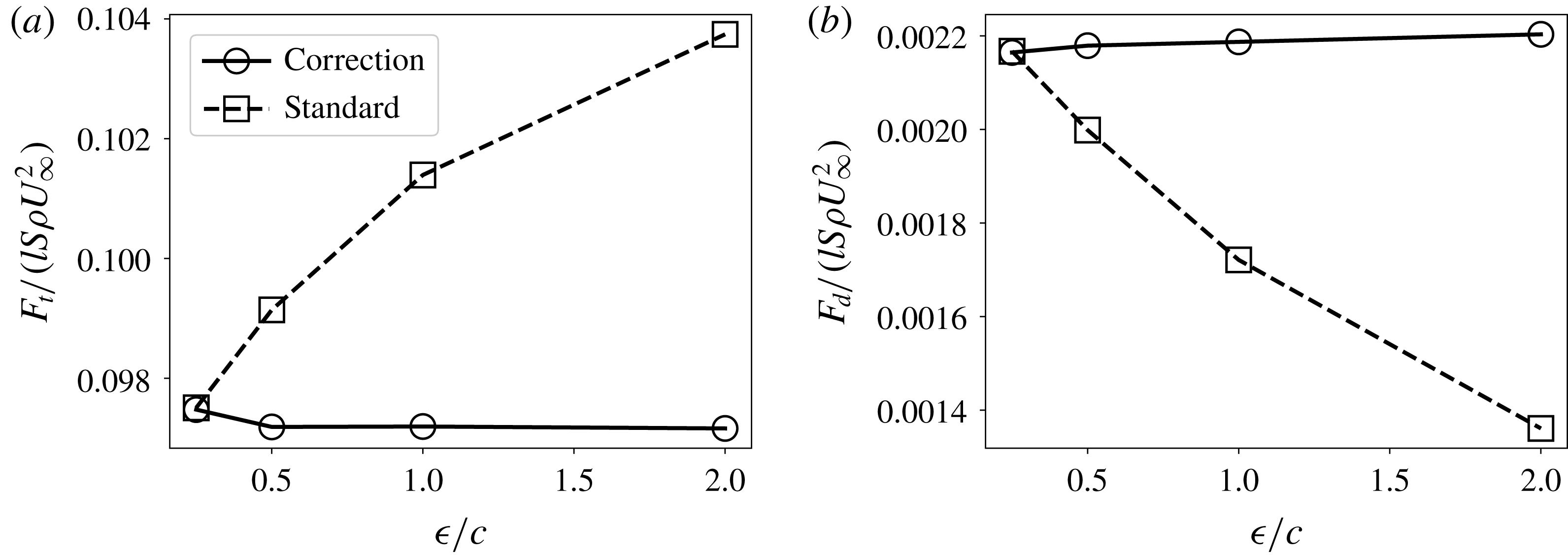
Total lift (a) and induced drag (b) for simulation of a constant chord wing (top) and one with elliptic chord distribution (bottom). Squares show results without using the subfilter-scale velocity correction; circles use the correction.