1. INTRODUCTION
Since the seminal works by Perron (1989, 1990) it has been well known that the performance of unit root tests is largely affected by the presence of structural level shifts, which, if neglected, tend to inflate the evidence in favor of a unit root. Busetti and Harvey (2001) and Busetti and Taylor (2003) report similar findings for the stationarity tests of, among others, Kwiatkowski, Phillips, Schmidt, and Shin (1992). A major debate in this strand of the literature has been on whether the possible shift date should be regarded as known or unknown. Among others, unit root tests robust to a level shift at a known date have been developed by Perron (1989, 1990), Amsler and Lee (1995), Saikkonen and Lütkepohl (2001), and Lanne, Lütkepohl, and Saikkonen (2002). Tests that allow for unknown shift dates have been initially proposed by Banerjee, Lumsdaine, and Stock (1992), Perron and Vogelsang (1992), and Zivot and Andrews (1992) and subsequently by Leybourne, Newbold, and Vougas (1998), Saikkonen and Lütkepohl (2002), and Lütkepohl, Saikkonen, and Trenkler (2004), among others; see Perron (2006) for a recent survey.
Few attempts have been made to robustify unit root tests in the presence of multiple level shifts. Lumsdaine and Papell (1997) and Clemente, Montañés, and Reyes (1998) generalize the tests proposed by Banerjee et al. (1992) by allowing for two level shifts at unknown dates. Unfortunately, there is little justification for fixing the number of shifts to one or two a priori (cf. Lumsdaine and Papell, 1997, p. 218), and the previously mentioned procedures can hardly be generalized to a larger number of shifts.1
An attempt has been made by Ohara (1999), who extended the Zivot and Andrews (1992) approach to the case of at most m breaks (m known). Size and power investigations (and also critical values) are presented for the two-break case only.
In this paper we take a novel approach to unit root testing in the presence of multiple level shifts. Specifically, we consider a rather general autoregressive data generating process (DGP) with additive level shifts having the following features: (i) level shifts occur randomly over time; (ii) the number of shifts is unknown and only needs to be bounded in probability; (iii) shifts need not occur independently over time and, in particular, may cluster together; (iv) shift sizes are random and of larger magnitude order than the shocks driving the autoregressive dynamics; (v) although shifts are exogenous throughout the paper, forms of dependence with the shocks driving the autoregressive dynamics could be allowed without affecting the results. These features differ in several respects from what has been previously considered in the literature. For instance, the investigator is not required to have any a priori knowledge about either the number or the location of shifts. The restrictions on the sequence of shift dates are mild, the main one being of technical nature and requiring the total number of shifts not to grow with the sample size. This is in contrast with a strand of the literature where the number of shifts diverges together with the number of observations (cf. Balke and Fomby, 1991a, 1991b; Franses and Haldrup, 1994; Nelson, Piger, and Zivot, 2001), but we adopt it to preserve in the limit the distinction between ordinary shocks and level shifts.2
In a recent paper, Perron and Qu (2004) adopted an approach similar to ours for evaluating the impact of structural breaks occurring randomly over time on log-periodogram estimation.
Despite the generality of (i)–(v), we are able to propose a family of ADF-type tests with null asymptotic distribution identical to that of ADF tests under standard conditions and, hence, without the need for new tables of critical values. Furthermore, the new tests have the same asymptotic local power function as standard ADF tests in the case of no level shifts.
Similarly to Amsler and Lee (1995) and Saikkonen and Lütkepohl (2002), the logic of the tests is to remove from the original time series, say, Xt, the level shifts that might have occurred over a given sample and then to apply standard ADF tests to the obtained “dejumped” time series, say,

. To remove the shifts, for each observation we suggest computing a probability

(with respect to an ad hoc postulated distribution) that a level shift has occurred at time t, given the data. Then, shifts are removed by defining

as

. ADF tests on

are found to have the same (pivotal) limiting distributions as standard ADF tests under no level shifts—a property that holds both under the unit root null hypothesis and under local alternatives.
The idea of weighting each observation with a (pseudo) probability is present in the work of Franses and Lucas (1998) on the robustification of cointegration tests to innovational outliers. Despite the similarity, we depart from a rather different statistical model, which gives rise to estimators and tests with different asymptotic properties. For example, although not required for the definition of the unit root tests, in our framework consistent estimation of the shift dates is feasible, in contrast with the framework of Franses and Lucas.
To evaluate the relevance of the asymptotic theory developed in this paper, the agreement of its predictions with the existing finite-sample evidence is worth noting. Specifically, we show that neglecting the level shifts affects the asymptotic local power of the ADF tests, which is consistent with the widely documented findings that in finite samples unit root tests lose power in the presence of level shifts.
A specificity of our probability analysis is that it relies on random fixed-point theory. Although it is a common practice to compute parameter estimates as fixed points of iterative algorithms, estimators themselves are rarely studied as fixed points; Aitchison and Silvey (1958) is a notable exception. By choosing a fixed-point approach, we can ensure that the object under analytical study is identical with the object that is actually computed—an obvious requirement that may otherwise be hard to check.3
For example, numerical techniques may deliver a local maximum of a criterion function, whereas the asymptotic analysis may have been carried out for a global one.
The paper is organized as follows. In Section 2 we present the reference DGP. We also discuss the asymptotic distributions of standard unit root tests in the presence of level shifts occurring independently over time, and we show that the distribution of the ADF statistics is characterized by a Poisson-type jump process, both under the null and under local alternatives. In Section 3 the proposed tests for unit roots in the presence of level shifts and their asymptotic properties are introduced and discussed. In Section 4 we refine our approach by proposing an algorithm for estimating the level-shift dates jointly with the parameters governing the autoregressive dynamics. The small-sample properties of the new tests are analyzed through a set of Monte Carlo simulations in Section 5. In Section 6 we discuss how the new tests can be implemented in the case of linear time trends and unknown autoregressive order. Section 7 concludes. Proofs are collected in the Appendix. The following notation is used:

denotes weak convergence and

convergence in P-probability, with OP(1) denoting boundedness in P-probability;

is the indicator function; Ik and 1k are the k × k identity matrix and the k × 1 vector of ones. With x := y (x =: y) we indicate that x is defined by y (y is defined by x), and [lfloor ]·[rfloor ] signifies the largest integer not greater than its argument. With

we denote the space of càdlàg functions on [0,1], endowed with the Skorohod topology. For a vector

, ∥x∥ := (x′x)1/2 stands for its euclidean norm, whereas for a matrix A, ∥A∥ := [tr(A′A)]1/2, where tr(·) is the trace operator. Finally, for any scalar sequence, e.g., {Xt}, ΔXt := Xt − Xt−1, ∇Xt := (ΔXt,…,ΔXt−k+1)′, and Xt := (Xt,(∇Xt)′)′.
2. MODEL AND PRELIMINARY RESULTS
2.1. Model and Assumptions
We are interested in testing the unit root null hypothesis

against local alternatives

and fixed alternatives

, in the following additive level-shift model for the observable variable Xt:

where Yt is an unobservable autoregressive process, Zt is a p × 1 vector of deterministic terms (e.g., a constant and a linear trend for p = 2), φ is a fixed vector conformable with Zt, and μt is an unobservable level-shift component. The following assumption is maintained.
Assumption

.
(a) The roots of

have modulus greater than 1;
(b) {εt}t=−k∞ is independent and identically distributed (i.i.d.) with zero mean, variance σε2 > 0, and E|ε1|r < ∞ for some r ≥ 4.
Assumption

prevents Yt from being I(2) or seasonally integrated, and it ensures that the so-called long-run variance of ut, hereafter σ2 := σε2Γ(1)−2, is well defined. The novelty of the paper lies in the way μt is specified and dealt with. To focus on this aspect, we regard the lag order k as known, and in the entire analytical part we consider the case φ = 0; the case φ ≠ 0 and also the case of unknown lag order are discussed in Section 6. Initial values are set to μ−k,…,μ0 = 0, and (u−2k,…,u−k−1)′ is given the stationary distribution induced by the difference equation

;
4The results of the paper remain valid under the more general specification u−2k,…,u−k−1 = OP(1).
In the absence of level shifts and deterministic terms, Xt = Yt holds for all t; in this case, if

and

denote, respectively, the ordinary least squares (OLS) estimators of α and γ := (γ1,…,γk)′ in the regression Xt = αXt−1 + γ′∇Xt−1 + errort, the well-known ADF unit root tests build on the statistics

and

, where

and

is the (OLS) standard error of

. Under Assumption

and for α = 1 − c/T (c ≥ 0), it is known (see, e.g., Phillips, 1988; Chang and Park, 2002) that

,

, and

as T → ∞, where

defines an Ornstein–Uhlenbeck process and B(·) is a standard Brownian motion. Under the null hypothesis that c = 0, Bc(·) = B(·), and the distributions in (2) are the univariate Dickey–Fuller distributions. Under the fixed alternative

, both

and ADFt diverge to −∞, and the unit root tests are consistent.
Now, suppose that the level-shift component μt is constant except for a few shifts. The simplest example is the single level-shift model, with the level-shift component changing from μ0 to μT at time T*, 0 < T* < T (cf. Perron, 1989; Amsler and Lee, 1995; Saikkonen and Lütkepohl, 2002, p. 316). This model corresponds to μt being generated as

with θ* denoting the magnitude of the level shift, or, equivalently, as

with δs a dummy variable equal to unity at the time T* of the level shift. Rather than assuming a single deterministic level shift, in this paper we consider shifts that occur randomly over time and have random magnitude. This is achieved by specifying the level-shift component as

where {δt} is an unobservable sequence of binary random variables indicating the occurrences of shifts and {θt} is the (random) sequence of shift sizes.
5As remarked earlier, we set μ0 = 0 in the following discussion.

, with NT denoting the total number of level shifts. The level shifts are assumed to have the following properties.
Assumption

.
(a) NT is bounded in probability conditionally on NT ≥ 1;
(b) θt = T1/2ηt, where {ηt}t=1T and {ηt−1}t=1T are sequences of OP(1) random variables as T → ∞;
(c) {δt}t=1T is independent of Y−k−1, (u−2k,…,u−k−1)′, {εt}t=−kT, and {ηt}t=1T for all T.
Several points are worth noting.
Remark 2.1. Formally, because {δt}, {θt}, and, under

, also α of (1) depend on T, we are considering a triangular array of the form {XT,t = YT,t + μT,t; t = −k,…,T, T = 1,2,…}. The magnitudes of the level shifts could also constitute an array {ηT,t; t = 1,…,T, T = 1,2,…} with the property that, for every ε ∈ (0,1), P(Mε ≥ |ηT,t| ≥ mε) > 1 − ε for some constants Mε ≥ mε > 0 and t = 1,…,T, T = 1,2,…; see Theorem 1 in Section 2.2. Unless differently specified, to keep notation simple we drop the T subscript.
Remark 2.2. Assumption

generalizes the simple single shift model (3)–(4) in a number of directions. Specifically, it allows for multiple level shifts, whose number NT only needs to be bounded in probability. This is a stochastic analogue of the deterministic setup in, among others, Perron (1989), where processes with a fixed number of structural breaks are studied. It is in contrast with the setup of, e.g., Balke and Fomby (1991a, 1991b) and Franses and Haldrup (1994), who let the number of level shifts diverge together with the sample size. Assumption

does not restrict the dependence structure of {δt} and, in particular, allows for clusters of level shifts (including shifts at consecutive dates).
Remark 2.3. Assumption

fixes the stochastic magnitude order of level-shift sizes at T1/2. It is not new; cf. Leybourne and Newbold (2000a, 2000b) and Perron (1989, p. 1372). This choice matches the stochastic magnitude order of {Yt} under the hypothesis α = 1 − c/T and implies that level shifts have a nonnegligible effect on the asymptotic distribution of ADF statistics, a desirable property given the broad evidence of a substantial effect on their finite-sample distributions. The rate of T1/2 has also been used by Müller and Elliott (2003) to model the initial observation of processes with roots near unity. Note that Assumption

imposes no restriction on the dependence structure of {ηt} and, hence, of shift sizes.
Remark 2.4. Assumption

specifies the occurrence of level shifts as exogenous. This is not a strictly necessary assumption for the results of the paper. Thus, if P denotes the sequence of probability measures induced by model (1) under Assumptions

and

, and conditional on the occurrence of at least one level shift (as will be imposed in Section 3), it holds that maxt:δt=1|εt| := max1≤t≤T|δtεt|, maxt:δt=1|ΔYt|, maxt:δt=1|ηt|, and maxt:δt=1|ηt−1| are bounded in P-probability. What matters in the proofs of the main results is this boundedness, and as long as a relaxation of

(such as the case of endogenous level shifts) does not affect it, the results of the paper continue to hold.
Remark 2.5. Our model can equivalently be expressed in the multiple-break format (see, e.g., Bai and Perron, 1998) with m := NT breaks and

where the break points Tj are obtained as Tj := max{t ∈ {1,…,T} : Nt < j}, with T0 := −k, Tm+1 := T, and μ(j) := μTj.
2.2. Effect of Level Shifts on ADF Tests
Our goal is to propose unit root tests with asymptotic distributions (2) under the full generality of Assumption

. In this section we argue that these tests cannot be the standard ADF tests, because under Assumption

their asymptotic distributions depend on nuisance quantities. To make this point, we do not need the full generality of the assumption; instead, for tractability, we introduce extra structure in the dependence and heterogeneity properties of the level shifts. The extra assumptions, which still represent a significant generalization of Leybourne and Newbold's (2000a) single shift setup, are maintained only in Section 2.2.
Let {δt} be serially independent and let

for t = 1,…,T, where G : [0,1] → [0,∞) is a continuous nondecreasing and not identically zero function with G(0) = 0. For example, if G(s) = λs (λ > 0 and T > λ), the case of time-independent shift-occurrence probability obtains: P(δt = 1) = λ/T. In general, however, the probability of shift occurrence can vary over time, as, e.g., in the case

, where P(δt = 1) equals zero and λ/T, respectively, in the first and the second half of the sample. Note that under the adopted specification the distance between consecutive level shifts increases with T.
6As is needed for convergence of T−1/2μ[lfloor ]T·[rfloor ] in

; cf. Example VI.1.20 of Jacod and Shiryaev (2003).

, where

is a continuous function,

, and {ωt}t=−∞T is i.i.d. with E|ω1| < ∞.
7Stochastic boundedness of {ηt−1}, as in Assumption

, requires further assumptions on F, {ψi}, and {ωt}. These are relevant to the detection of level shifts but not to Theorem 1, and so we omit them.

could be the stationary solution of an autoregressive equation. The so defined {ηt} is, in general, weakly serially dependent and has time-varying dispersion driven by F(·) (see, e.g., Cavaliere, 2004) but can also be i.i.d. as a special case. Asymptotics for the ADF statistics under this specification are given in Theorem 1, where

denotes a Poisson process with intensity G. The process

is defined on [0,1] and is constant apart from finitely many jumps equal to one. Recall that σ2 denotes the long-run variance of ut.
THEOREM 1. Let Assumption

be satisfied and let θt be specified as above, with {δt}t=1T, {ωt}t=−∞T, and {εt}t=−kT jointly independent and independent of Y−k−1 and (u−2k,…,u−k−1)′. Then, under

and

, the following convergence holds in

as T → ∞:

where Bc and

are independent stochastic processes, Bc is an Ornstein–Uhlenbeck process with parameter c,

is the nonhomogeneous compound Poisson process

, with {ηi*} i.i.d., distributed as η1, and independent of

and with

denoting the sequence of jump times of

. Moreover,

where ϰ0 and ϰ1 depend on

, with

standing for the quadratic variation of

over [0,1]. For k = 0 we have ϰ0 = 0 and

, whereas for any k, ϰ0 = 0 and ϰ1 = 1 conditionally on

.
8The expressions for ϰ0 and ϰ1 for arbitrary k are given in the Appendix, sect. A.2.2.
In Theorem 1 two effects of level shifts on the asymptotic distribution of ADF statistics under

and

can be disentangled. First, in (6) the weak limit

of the level-shift process T−1/2μ[lfloor ]T·[rfloor ] is superimposed on the weak limit Bc(·) of T−1/2Y[lfloor ]T·[rfloor ], in the same way as μt is superimposed on Yt in finite samples. As a consequence,

appears in (7) instead of Bc(·). Second, outliers in the first differences of Xt (induced by shifts in the levels) give rise to ϰ0 ≠ 0 and ϰ1 ≠ 1. For k = 0 the only effect is through outliers in the regressand ΔXt; they lead to inconsistent estimation of σε2 = Var(εt) and, thus, to ϰ1 ≠ 1. For k > 0, outliers in the lags of ΔXt lead to inconsistent estimation of γ and also affect the limiting distribution of

; hence, the appearance of ϰ0 ≠ 0 and the more involved expression for ϰ1. The difference between (7) and the Dickey–Fuller distributions (2) arising in the absence of shifts agrees with the different finite-sample performance of ADF tests in the two cases, most notably under local alternatives, where level shifts lead to substantial power losses. The Monte Carlo simulations in Section 5 illustrate this aspect.
Remark 2.6. A simple special case of distributions (7) obtains when ηt = ωt = η is fixed (shift sizes are identical), F ≡ 1, and G(s) = λs for some λ > 0 and T > λ. Then

is a time-homogeneous Poisson process,

is replaced by ;

in (6) and (7), and

is replaced by

. The importance of the Poisson component depends on the size of the level shifts relative to the long-run variance of the errors (through η/σ) and also on the intensity of occurrence of level shifts. When the level shifts are small, i.e., η/σ is close to zero, the limiting distributions in (7) are close to the usual Dickey–Fuller type distributions. Conversely, when the shifts are large, the Poisson component becomes dominant.
Remark 2.7. The functional convergence

in

generalizes Theorem 3.1 of Leipus and Viano (2003) to a setup where the jumps of the finite-sample process can be weakly dependent and heteroskedastic. The jumps of the limiting process

are independent regardless, because the jumps of T−1/2μt are sampled from {ηt} at intervals whose length diverges as T → ∞ and because the dependence between the terms of {ηt} vanishes as the time distance between them grows without bound. Functional convergence to

leads to Lemma A.3 in the Appendix, which contains (univariate) generalizations of product-moment convergences of Georgiev (2008) and underlies (7). For k = 0, {ηt} i.i.d., and F ≡ 1, in (7) convergence of the ADFt statistic under the unit root hypothesis follows by specializing the discussion of Georgiev (2008, Sect. 3) to the univariate case.
Remark 2.8. From the proof of Theorem 1 in the Appendix it follows that for a fixed α ∈ (−1,1) the convergence

holds in

; cf. (6). Thus, X[lfloor ]T·[rfloor ] has the same stochastic magnitude order under

and

. As a consequence, by modifying the proof of Theorem 1 it can be shown that in our setup ADF tests are not consistent against fixed alternatives; cf. Leybourne and Newbold (2000b, Cor. 1).
3. TESTS THAT ACCOUNT FOR THE LEVEL SHIFTS
3.1. Overview
Given the conclusion of Theorem 1 that, in the presence of level shifts, the ADF statistics based on the observed time series Xt do not have the usual asymptotic distributions (2), here we propose modified statistics that do have (2) as their asymptotic distributions. Two powerful implications are that, first, standard tables of asymptotic critical values can be used for the proposed tests and, second, whatever the number and the size of the shifts are, these tests have the same asymptotic local power as ADF tests in the absence of shifts.
Recall that, under Assumption

, the asymptotic distributions of the ADF statistics from the regression Yt = αYt−1 + γ′∇Yt−1 + errort are as given in (2). However, because Yt is unobservable, this regression is not feasible empirically. Because Yt = Xt − μt can be thought of as obtained from Xt by removing the (also unobservable) level shifts, we propose conducting ADF tests on a process obtained by subtracting from Xt an estimator of μt. The idea is related to the work of Saikkonen and Lütkepohl (2002), who suggest adjusting the original time series by removing an estimator of its deterministic component, including possible (deterministic) level shifts. Because in our case μt is a random jump process, in what follows our procedure is referred to as “dejumping.”
If δt were observable, but the shift sizes not, to optimize test power under alternatives close to the null we could estimate the shift sizes by pseudo–generalized least squares (pseudo-GLS) under local alternatives, as suggested by Elliott et al. (1996). Furthermore, to keep under control the finite-sample size of the resulting tests, following the suggestion of Saikkonen and Lütkepohl (2002) and Lanne et al. (2002), we would set the localizing parameter to zero. This reduces to estimation of shift sizes under the unit root null, i.e., to a regression of ΔXt on impulse dummy variables, one per shift. The implied estimator of μt would be

The estimation error

is bounded in probability uniformly in t (see Lemma A.2 in the Appendix), whereas μt (and also Yt under

and

) has stochastic magnitude order T1/2. This difference turns out to be sufficient for the ADF statistics based on the “dejumped” series

to have the null and local-to-null asymptotic distributions given in (2) and to diverge under fixed alternatives.
In the case of unobservable δt we imitate the preceding dejumping scheme through the following three-step procedure:
- the sequence of level-shift indicators {δt} is consistently estimated by an estimator
; the level-shift component is estimated by
 ;
- the level shifts are removed by constructing the dejumped series
and;
- standard ADF tests, say,
and ADFtδ, are computed usinginstead of the original time series; the unit root null hypothesis is evaluated by comparingand ADFtδ to standard asymptotic critical values (see, e.g., Fuller, 1976).


In this framework, the key step is the consistent estimation of level-shift indicators. Specifically, because

, for the ADF test obtained from the preceding steps 1–3 not to be influenced asymptotically by the fact that δt are estimated,

should converge to zero sufficiently fast. In the Section 3.2 we propose an estimator

with this property; it is the expectation of δt conditional on the data, with respect to an ad hoc postulated distribution. This estimator offers the flexibility of not requiring an explicit decision rule about the location of shifts, although as a by-product it gives rise to such a rule with a traditional interpretation.
3.2. Level-Shift Estimation and Unit Root Tests
Our proposed level-shift estimation method starts by noticing that the distribution of ΔXt is a mixture, with mixing variable δt and mixture components
9Although we write as if the two component distributions are the same for all t, in general they constitute a family indexed by t (e.g., ηt does not need to be identically distributed over time).

the mixture components have different orders of magnitude, they are “well separated,” and consistent classification is feasible.
In the spirit of quasi maximum likelihood (QML) estimation,10
The level-shift estimator is inspired by the specification in Remark 2.6; nevertheless, all the results in what follows hold in the more general setup of Assumption

.

where t(ν) denotes a Student t-distribution with ν degrees of freedom. The corresponding quasi likelihood function for λ, when σ2 and η2 are regarded as known, is

where, for a > 0, φν(e;a2) is the probability density function of a·t(ν). The QML estimator of λ then satisfies the equation

with

We abbreviate

to

. Note that

, with

denoting expectation conditional on the data under distribution (8). Thus,

measures how likely it is, given the data and the postulated distribution, that a level shift occurred in period t.
From (9) it follows that, for fixed σ2 and η2, the QML estimator of λ is a fixed point of the map

. This allows us to retrieve the estimator of the level-shift indicators straightforwardly. First, the fixed point can be computed by iterating the map until convergence. Second, the resulting estimate of λ can be inserted into (10), yielding the estimates of δt needed to eliminate the level shifts from the original time series.
The pseudo parameters η2 and σ2 are related to the squared magnitude of the draws from the mixture components, respectively,

and

. Thus, instead of fixing η2 and σ2 a priori, we suggest replacing them with

The estimator of {δt}t=1T is then obtained as

, where ζT is a random fixed point of the random map ΦT obtained by combining equations (9) and (11):

Once ζT has been found, level shifts can be removed from Xt by computing the series

,

, and the unit root hypothesis can be tested by conducting standard ADF tests, henceforth

and ADFtδ, on the ADF regression

(recall that

). In Section 3.3 we show that

estimate δt consistently at a rate fast enough for

and ADFtδ to have the usual Dickey–Fuller type asymptotic distributions under the null and under local alternatives. Under fixed alternatives the statistics give rise to a consistent test.
Remark 3.1. The graph of

as a function of |e| is an S-curve starting at λ/T for e = 0 and approaching unity as |e| → ∞. For larger values of ν in (8), the curve is closer to that of a step function, in the sense that it remains closer to zero for small |e|, exhibits steeper increase for intermediate values of |e|, and is closer to one for large |e|. As extensive simulations have shown, larger values of ν translate into a more sensitive estimator of {δt} in finite samples and into unit root tests with better finite-sample power. We found no further power gains associated with the use of binary 0-1 estimators instead of our smooth estimators

. That is, a 0-1 estimator defined as equal to unity if and only if

, κ ∈ (0,1), induces for some values of κ tests with power comparable to that of a smooth estimator with large ν, whereas for other values of κ the 0-1 estimator yields lower power. Moreover, the optimal value of κ depends on the DGP. For these reasons, we prefer to base our tests on the smooth estimators.
Remark 3.2. Recall that, under model (1), a level shift occurring at time t generates a large outlier in the differenced series ΔXt. Hence, an approach alternative to our smooth level-shift estimation is the application to ΔXt of traditional outlier detection methods (see, e.g., Chen and Tiao, 1990; Chen and Liu, 1993, and references therein). Simulations have shown that implementation of these methods in conjunction with dejumping results in oversized tests, with no gains in size-adjusted power. Interestingly, our approach can, but need not, operate as a traditional method. Traditional methods typically classify as outliers regression residuals that, upon standardization, exceed some threshold. In our framework, the inequality

, κ ∈ (0,1), is equivalent to |e/σ| > τT,ν(κ,λ,η/σ), for a function τT,ν that can be found explicitly. Hence, if we evaluate

at a regression residual, as we essentially do in Section 4, and compare the value to a threshold κ, this is equivalent to a comparison of the standardized residual to a threshold depending on κ, on the occurrence intensity of shifts, and on their relative size. As mentioned in the previous remark, in terms of test properties, there seems to be little payoff to the complication of choosing an appropriate κ.
Remark 3.3. As our model can be cast within the multiple-break format (5), another approach to the estimation of level-shift dates is the procedure of Bai and Perron (1998). Again, extensive Monte Carlo experiments have shown that in our framework this procedure does very well in detecting the correct level-shift dates under fixed alternatives, with unit root tests based on Bai–Perron dejumping having power properties comparable to ours. However, in our experience unit root tests based on Bai–Perron dejumping tend to have worse size properties and, under local alternatives, worse size-adjusted power.11
A possible explanation for this result is that the Bai–Perron procedure delivers unsatisfactory results when the level-shift component μt and the (near-) integrated component Yt are both of order OP(T1/2), as in our model under the null hypothesis and under local alternatives.
3.3. Asymptotic Results
We start this section with a theorem about existence, uniqueness, and asymptotics for a fixed point ζT of the mapping ΦT (see expression (12)), such that the estimator of the level-shift indicators

is consistent for δt uniformly in t.
12It is straightforward that ΦT also has the trivial fixed point

, which however fails to satisfy the consistency requirement.
THEOREM 2. Let P be the probability measure induced, under Assumptions

and

, by model (1) with either α = 1 − c/T (c ≥ 0) or α = α* ∈ (−1,1), and conditional on the realization of at least one level shift. If ν of (8) satisfies 3 ≤ ν ≤ r − 1, then we have the following results as T → ∞:
(i) Existence. There exists a random sequence {ζT} such that P(ΦT(ζT) = ζT) → 1, ζT = OP(1), and ζT is componentwise bounded away from zero in P-probability.
(ii) Uniqueness. If ζT and ςT both have the preceding properties, then P(ζT = ςT) → 1.
(iii) Computability. For every nonrandom ζT0 with positive coordinates, the sequence of iterates ζTi := ΦT(ζT,i−1), i ≥ 1, satisfies P(ζTi →i→∞ ζT) → 1.
(iv) Consistency.

,

, and ζT = (NT,HT,σY2) + oP(1), where

and σY2 := P limT→∞ Var(ΔYT).
Thus, ζT is consistent for (NT,HT,σY2), and

is consistent for the sequence of level-shift indicators {δt}t=1T at the rate of T1/2. As a consequence (not used in the discussion that follows), for any sequence aT = const ∈ (0,1) or aT = Tε−1/2, 0 < ε < ½, the set of periods with

coincides, with P-probability approaching one, with the set of periods where level shifts occur. This is a consistent explicit level-shift detection rule.
Remark 3.4. Adopt the notation z = (zλ,zη,zσ)′ for vectors

. According to the consistency part of Theorem 2, (ζTλ,ζTη) = (NT,HT) + oP(1). This introduces a small complication into the argument for existence of ζT, for in general no compact in

contains NT and HT (and, hence, (ζTλ,ζTη)) with probability approaching one, whereas existence theorems for random fixed points are typically formulated for self-maps of compacts. One consequence is that to prove the theorem we resort to the trick of looking for a fixed point of the form ζT = ζ(zT), where ζ is the random function ζ(z) = (NT + zλ,HTzη,zσ)′ and (zTλ,zTη) = (0,1) + oP(1). For HT ≠ 0 the inverse function ζ−1 is well defined, and zT can be found as a fixed point of ζ−1 ○ ΦT ○ ζ. To ensure that we can avail ourselves of this fact, Theorem 2 is stated conditionally on the presence of level shifts (NT ≥ 1), so that HT ≠ 0 a.s. The case NT = 0 is considered in the simulation exercise in Section 5.
Before introducing in Theorem 3 our main result, we present an important lemma that forms the basis of the proofs of both Theorems 2 and 3. The lemma contains several convergence statements uniform on compacts. One is in regard to the rates of consistent estimation of {δt}; another one concerns the distance between the OLS estimators of α and γ from ADF regressions for dejumped series and for the unobserved Yt; yet another statement is an evaluation of the Jacobian matrix of ΦT that underlies contraction arguments. In the lemma, for compacts

in

and real functions f defined on

, we write

as

.
LEMMA 1. Let ζ be the identity function on

or the random function defined by ζ(z) := (NT + zλ,HTzη,zσ)′, and let the compact

be such that

and

are bounded away from zero in P-probability, υ ∈ {λ, η, σ}. Define

, Xtδ := Xt (t = −k,…,0) and let ∇Xtδ be defined accordingly. Under the conditions of Theorem 2, it holds that
(i)

and

;
(ii)

;
(iii)

and

if α = 1 − c/T (c ≥ 0), where

,

, and

(αδ, γδ, and σε, δ2) are the OLS estimators of α, γ, and σε2 from the regression Yt = αYt−1 + γ′∇Yt−1 + errort (Xtδ = αXt−1δ + γ′∇Xt−1δ + errort);
(iv)

, where (ΦT)ς′ is the Jacobian matrix of ΦT(ς).
Remark 3.5. Throughout, the random functions appearing in suprema, infima, maxima, and minima are continuous and have separable domains (subsets of

). Hence, the extrema in question are random variables.
Remark 3.6. The lemma states that the OLS estimators of α and γ based on dejumped data and on the unobservable Yt are asymptotically equivalent under the null and under local alternatives. Asymptotic equivalence holds for any z belonging to any

, not only for a fixed point of ζ−1 ○ ΦT ○ ζ. However, because the fixed point matches relevant sample characteristics, it can be expected that a test based on it has better finite-sample properties. As can be seen from the proof of Lemma A.7 in the Appendix, under fixed alternatives αδ and γδ are asymptotically equivalent to the OLS estimators from the unfeasible regression for data dejumped with the true {δt} instead of

(

in the notation of Section 3.1) but not to the estimators from a regression for Yt. This is not surprising given that dejumping was aimed at optimizing test properties close to the unit root null. A similar phenomenon, which does not compromise the consistency of the tests, can be seen in the proof of Theorem 4.2 of Saikkonen and Lütkepohl (2002).
We are now ready to state our main result.
THEOREM 3. Suppose that the conditions of Theorem 2 are satisfied. Let ζT be as in Theorem 2 and let

denote Xtδ of Lemma 1 evaluated at ζT. Under

and

, the ADF statistics

, ADFtδ based on the regression

have asymptotic distributions given by (2); i.e., as T → ∞

where weak convergence refers to the sequence of measures conditional on NT ≥ 1. Under

,

and

as T → ∞.
According to Theorem 3, in the presence of level shifts the asymptotic distribution of the ADF statistics based on the dejumped time series

is the same as that of standard ADF statistics computed from series with no level shifts, both under the null and under local alternatives. This result allows us to refer to well-known tables of critical values (cf., e.g., Fuller, 1976). Moreover, under fixed alternatives the proposed tests are consistent.
4. JOINT ESTIMATION OF MODEL PARAMETERS AND LEVEL-SHIFT INDICATORS
The unit root tests described earlier are based on a sequential procedure: initially, level-shift indicators δt are estimated by looking at the observable increments ΔXt = ΔYt + θtδt; later, the parameters of model (1) are estimated by an ADF regression on the dejumped series. In this section we discuss a procedure for joint estimation of level-shift indicators and model parameters. Interest is not in parameter estimation per se but rather in the possibility of obtaining estimates of δt based on estimates of the disturbances εt + δtθt, instead of ΔYt + δtθt. As εt has smaller variance than ΔYt, εt and εt + θt are better separated than ΔYt and ΔYt + θt, and so the joint procedure can be expected to have better finite-sample properties than the sequential one.
In our setup, the joint estimation problem can be solved computationally by means of an iterative procedure based on the following steps: (i) estimation of level-shift indicators (where, at the first iteration, the estimates obtained from the basic estimation procedure (see Section 3.2) are used); (ii) construction of a dejumped time series; (iii) estimation of the regression coefficients α and γ by a standard ADF regression on the dejumped series; (iv) computation of estimates of εt + θtδt. These estimates serve as a new input for step (i), and the procedure is iterated until convergence. The unit root test statistics are computed within this procedure at step (iii).
Like the basic dejumping of Section 3.2, the preceding procedure delivers a fixed point, say, ξT, of a random map, say, ΨT. Compared to ΦT from (12), ΨT is of larger and sample-dependent dimension, as it has components for the parameters α and γ, and also for each δt, t = 1,…,T. The definition follows.
For a given d = (d1,…,dT)′, denote the process Xt dejumped with weights d by

and Xtd := Xt (t = −k,…,0), so that Xtd := (Xtd,(∇Xtd)′)′ (t ≥ 0) as agreed in Section 1. Further, for a given (a,γ′), let etd := ΔXt − (a,γ′)DTXt−1d (t ≥ 1), where a is inserted for T1/2(α − 1) and DT is the diagonal (k + 1) × (k + 1) matrix diag(T−1/2,1,…,1). Define ΨT, with argument ξ := (d′,a,γ′,λ,η2,σ2)′ and with components ΨTδ, ΨTa,γ, ΨTλ, ΨTη, and ΨTσ, as follows. First, let ΨTδ := (ΨT1δ,…,ΨTTδ)′,

for t = 1,…,T (see equation (10)) and

. Denote the series Xt dejumped with ΨTδ(ξ) by

and XtΨ := Xt (t = −k,…,0); for XtΨ defined accordingly, let ΨTa,γ(ξ) = (ΨTa(ξ), (ΨTγ(ξ))′) be the estimator of (aΨ,(γΨ)′)′ from the regression

Finally, using etΨ := ΔXt − (ΨTa,γ)′DTXt−1Ψ as an updated estimator of εt + δtθt, define

For a fixed point ξT of ΨT, consider the ADF statistics, say,

and ADFtΨ, from regression (13) for XtΨ evaluated at ξ = ξT. The next theorem addresses the existence and uniqueness of a random fixed point ξT such that ΨTtδ(ξT) estimate δt consistently and the statistics

and ADFtΨ have the usual asymptotic distributions (2) under the null hypothesis and under local alternatives.
THEOREM 4. Let the conditions of Theorem 2 hold. Then, under hypotheses

and

, there exists a random sequence {ξT} with the following properties.
(i) Fixed point property. P(ΨT(ξT) = ξT) → 1.
(ii) Consistency. {ΨTtδ(ξT)} estimate {δt} consistently:

and

, whereas ((ΨTγ(ξT))′,ΨTλ(ξT),ΨTη(ξT),ΨTσ(ξT)) = (γ′,NT,HT,σε2) + oP(1).
(iii) Unit root tests. The limiting distributions of

and ADFtΨ are given by

where weak convergence refers to the sequence of measures conditional on NT ≥ 1.
Furthermore, if part (b) of Assumption

is replaced by the requirement that E|ε1|r < ∞ for some r ≥ 5, then for 4 ≤ ν ≤ r − 1 the following facts hold:
(iv) Uniqueness. If ξT and ςT have properties (i)–(iii), then P(ξT = ςT) → 1.
(v) Computability. Let

and

with ζT as in Theorem 2 and

obtained from the regression in Theorem 3. Also let ξTi := ΨT(ξT,i−1) for i ≥ 1. Then P(ξTi →i→∞ ξT) → 1 as T → ∞.
Remark 4.1. The theorem is similar to Theorems 2 and 3 but weaker in some respects. Uniqueness is established within a smaller class of sequences than in Theorem 2, but this has no practical implications, given that the iterative algorithm from Theorem 4(v) converges to the fixed point ξT with properties (i)–(iii). The choice of initial value for the iteration is important: Theorems 2 and 3 ensure that ξT0, defined through the fixed point of the basic dejumping procedure, is sufficiently close to ξT for the iteration to converge.
Remark 4.2. Theorem 4 does not cover fixed alternatives, which are studied in the next section by simulation.
5. MONTE CARLO RESULTS
In this section the finite-sample size and power properties of standard ADF tests

and of the proposed ADF tests based on level-shifts removal are investigated by Monte Carlo simulation for DGPs either with or without level shifts. We need to establish two main facts: first, that allowing for multiple level shifts does not result in deteriorated size properties of the new tests; second, that the power properties of the new tests are close to those of the usual ADF tests under standard conditions (i.e., without level shifts), at least as the sample size increases, under fixed and local alternatives. Additional aspects of interest are how the new tests behave when the magnitude of the level shifts is independent of T and how the properties of the tests are affected by the choice of the degrees of freedom ν in (8). In particular, we want to assess whether the bounds on ν in Theorems 2–4 are strict. Finally, the section ends with a study of the single shift case in which our tests are compared to some well-known unit root tests especially developed to deal with a single shift. We aim at showing that not using the prior information on the number of shifts (which in practice is available only by exception) does not necessarily entail power losses for our tests.
The employed DGPs are as follows. Data are generated for sample sizes of T = 100,200,400 observations according to model (1) with k = 1, γ := γ1 ∈ {−0.5,0,0.5}, φ = 0, Y−1 = 0, and zero-mean unit-variance i.i.d. innovations, following either a Gaussian or a standardized t(10) distribution. We consider the unit root case, which obtains by setting α = 1 in (1), the sequence of local alternatives α = 1 − c/T with c := 7, and the fixed alternative α = 0.9.
Three specifications of the level-shift component are initially employed. First, the case of no level shifts (μt = 0 for all t) is considered, with the resulting model denoted by S0. Second, with S4 we denote the case of four shifts occurring at fixed sample fractions ti, i = 1,…,4, with t1 := [lfloor ]0.2T[rfloor ], t2 := [lfloor ]0.35T[rfloor ], t3 := [lfloor ]0.6T[rfloor ], and t4 := [lfloor ]0.8T[rfloor ] and with size magnitudes η1 = η4 := 0.4 and η2 = −η3 := 0.35; consequently, the level shift component is13
For our selection of T, this model generates level shifts of size between 4 and 8 standard deviations of the errors. These shift magnitudes, although large, are not unrealistic. For instance, Vogelsang and Perron (1998, p. 1090) report, for the long gross national product (GNP) series considered in Perron (1992), level shifts “generally no larger (in absolute value) than 8 … relative to the standard deviation of the innovation errors.” Furthermore, in some recent papers (see, among others, Papell, Murray, and Ghiblawi, 2000), unit root tests under level shifts are applied to unemployment series where level shifts are as large as 10 times the standard deviation of the innovations. Using, as in Perron (1990), quarterly U.S. unemployment data from 1948 to 1988 with a break at 1974:1, we have estimated the size of the shift as 6.9 times the residual standard deviation from a 9 lags ADF regression on the dejumped data (cf. Perron, 1990, Table 1). With T = 163 this corresponds to η = 0.54, which is actually larger than the values we have used in our Monte Carlo design. Similarly, using monthly unemployment over the same range (T = 485) we find that the size of the shift is 10.4 times the residual standard deviation from the second-stage ADF regression; this corresponds to η = 0.47.

Third, we consider a case, Sr in the following discussion, with a random number of level shifts NT ∼ 2 + B(T,2/T) (B denoting a binomial distribution); i.e., at least two, and on average four, level shifts occur over the sample. The shift dates ti, i = 1,…,NT, are generated as ti := [lfloor ]τiT[rfloor ], where the relative locations τi are independent and uniformly distributed on [0,1]; the (independent) shift sizes ηt are drawn from a uniform distribution on [−4,−0.35] ∪ [0.35,4].
We consider tests based both on the basic dejumping procedure

(see Section 3) and on the “finer” version of Section 4

. For the degrees of freedom parameter ν of (8), in the Gaussian case Theorems 2–4 allow us to choose arbitrarily large finite values. We have checked that the simulation results for large finite ν are, first, virtually indistinguishable from those for ν = ∞ (i.e., standard Gaussian densities instead of t densities in (8)) and, second, yield best test performance. Thus, in what follows we set ν = ∞ in the case of Gaussian innovations. In the case of standardized t(10) innovations, to investigate the relevance of the upper bound on ν in Theorems 2–4 we use both ν = 8 (which satisfies the bound ν ≤ r − 1) and ν = ∞ (which violates it). All tests are performed at the 5% (asymptotic) nominal level, with critical values taken from Fuller (1976, Tables 10.A.1 and 10.A.2). Computations are based on 10,000 Monte Carlo replications and are carried out in Ox v. 3.40 (Doornik, 2001).
Size.
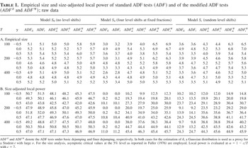
In Table 1A we report the finite-sample size of the six considered tests for Gaussian innovations. Two results are worth noting. First, in the case of no level shifts (model S0) the size properties of the proposed tests are accurate, with sizes ranging from 4.8% to 5.5% for the ADFδ tests (basic dejumping) and from 4.9% to 6.0% for the ADFΨ tests (finer dejumping). Hence, allowing for multiple level shifts does not result in spurious rejection of the unit root hypothesis. Second, in the case of multiple level shifts (models S4 and Sr) standard ADF tests tend to be slightly undersized, in particular for γ = ±0.5.14
This result agrees with the asymptotics of Section 2, where it is shown (i) that in the presence of level shifts standard unit root tests do not behave according to the standard asymptotic theory even under the null hypothesis and (ii) that the ADF test statistics are no longer invariant to the short-run parameters γ.
Empirical size and size-adjusted local power of standard ADF tests (ADF) and of the modified ADF tests (ADFδ and ADFΨ); raw data

Power against Local Alternatives.
In Table 1B the size-adjusted power of the six tests is investigated under the local alternative α = 1 − 7/T, still for Gaussian innovations. In the case of no level shifts the new tests have roughly the same power properties as standard ADF tests. That is, allowing for level shifts when there are actually none does not cause the power properties of the tests to deteriorate. The picture changes when level shifts occur. For model S4, standard ADF tests have extremely low power: with T = 100, power is about 0 for γ = −0.5, about 0.2% for γ = 0, and about 10% for γ = 0.5 (in agreement with Theorem 1, the distribution of the ADF tests depends both on γ and on the level-shift process). Conversely, the tests based on dejumping have good power properties, with power growing toward the asymptotic power envelope as the sample size increases. For T = 100, power is about 10% for γ = −0.5, 20% for γ = 0, and 30% for γ = 0.5; for T = 200, power grows above 20% for γ = −0.5, 30% for γ = 0, and 40% for γ = 0.5. For T = 400, the rejection rate is about 38% for negative γ and 45% for γ ∈ {0,0.5}. The unit root tests based on the finer dejumping (ADFΨ) seem to be preferable over the tests based on the basic dejumping (ADFδ) for small sample sizes, as expected. Notice also that the dependence of finite-sample power on γ diminishes as T increases, as predicted by the asymptotic results of Sections 3 and 4. Results for the random shift model Sr do not qualitatively differ from those for the S4 model; in general, the power loss experienced by standard ADF tests is less severe than for S4, and the power of our tests is closer to the asymptotic power envelope. Overall, the power results are promising, as they show that we are able to distinguish between unit root processes and processes that are stationary apart from several level shifts, even in samples of moderate dimension.
Power against Fixed Alternatives.
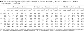
Table 2 reports the (size-adjusted) power of both standard and our unit root tests against the fixed alternative α = 0.9. In the case of no level shifts (model S0), the power of our test is close to the power of a standard unit root test; hence, there is no particular disadvantage in using the unit root tests that are robust to level shifts even if no shifts occur. For model S4, standard ADF tests have (size-adjusted) power close to zero, even for large sample sizes. Conversely, ADFδ and ADFΨ tests have power that significantly increases with the sample size. As in the case of local alternatives, large sample sizes are needed for the tests to achieve a power level close to that of ADF tests under no level shifts. Interestingly, the tests based on the joint estimation of the level-shift indicators and the autoregressive parameters (ADFΨ) have higher power than the tests based on the basic dejumping (ADFδ) when γ is negative. Results for the random level-shifts model Sr do not substantially differ, except that standard ADF tests now have nonzero power. For fixed alternatives that are further away from the null hypothesis, these results remain unchanged except that the joint estimation of the level-shift indicators and the autoregressive parameters now allows us to achieve better power properties in samples of moderate size.15
It has been recently noticed that for some unit root tests, power can decrease as α diverges from one; see Perron and Qu (2007) and references therein. To assess whether this drawback affects our tests also, we have run some Monte Carlo simulations based on model S4 for various values of α, γ, and T. The results show that the power reversal problem does not seriously affect our tests. More specifically, although the size-adjusted power is not monotonic in α, power tends to stabilize as α declines, in particular for the test based on the finer dejumping method of Section 4. Moreover, there is no evidence that, for values of α far away from the null, power tends to be very small. In general, the tests based on finer dejumping have the best power properties. The full set of results is available in the accompanying working paper, Cavaliere and Georgiev (2006), or from the Web page http://www2.stat.unibo.it/cavaliere/lshifts.
Size-adjusted power against fixed alternatives of standard ADF tests (ADF) and of the modified ADF tests (ADFδ and ADFΨ); raw data

Fixed Shift Sizes.
Although our paper deals with large level shifts, modeled as proportional to T1/2, here we briefly compare the properties of standard unit root tests and of the proposed tests when the size of the level shifts is kept fixed as T increases. To this aim, we consider the following modification of model S4:

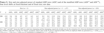
For T = 100, it generates exactly the level-shift component (14) analyzed so far, whereas for larger sample sizes, (15) generates shifts of smaller magnitude with respect to (14). Table 3 reports size, local power, and nonlocal power for T = 200,400; results for T = 100 are given in Tables 1 and 2, model S4. The following results are worth noting. First, although the impact of the level shifts decreases as the sample size increases, the power of standard ADF tests is still very low. Size distortions, however, are ameliorated. Second, the local power of the proposed ADFδ, ADFΨ tests still tends to the power envelope in the case of no shifts, although more slowly than in the case of large level shifts, as expected. Third, the power of the proposed tests grows as the sample size increases.
Size and size-adjusted power of standard ADF tests (ADF) and of the modified ADF tests (ADFδ and ADFΨ), four level shifts at fixed fractions and of fixed size; raw data

Student-t Innovations and the Choice of ν.
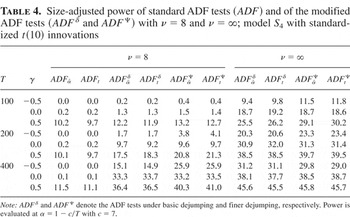
We now examine the properties of the tests when the innovations, instead of being Gaussian, follow a standardized Student t(10) distribution. The ADFδ and ADFΨ statistics are computed using ν = 8 (satisfying the assumption ν ≤ r − 1 of Theorems 3 and 4) and ν = ∞ (violating this assumption). Only the size-adjusted power under model S4 is reported in Table 4.16
Extended tables covering both size and power under models S0,S4 and Sr are available in Cavaliere and Georgiev (2006) or from the Web page http://www2.stat.unibo.it/cavaliere/lshifts.
This choice may not be optimal in the absence of level shifts; see the S0 panel referred to in note 16.
Size-adjusted power of standard ADF tests (ADF) and of the modified ADF tests (ADFδ and ADFΨ) with ν = 8 and ν = ∞; model S4 with standardized t(10) innovations

Single Level Shift and Comparison with Existing Tests.
As anticipated at the beginning of this section, we aim at comparing the proposed tests with existing methods in the well studied case of a single level shift; see Perron (2006) and Vogelsang and Perron (1998) for a review. Specifically, we consider the following tests for a unit root under a level shift at an unknown date: (i) the test proposed by Perron and Vogelsang (1992), ADFtPV hereafter; (ii) its “efficient” generalization based on GLS removal of the level shifts, as proposed by Perron and Rodriguez (2003), denoted as ADFtPR.18
We do not compare our tests with tests designed for the case of two level shifts (e.g., Lumsdaine and Papell, 1997; Clemente et al., 1998) because these tests do not outperform their single-break counterparts (i.e, the ADFtPV test) when there is only a single level shift. We also avoid comparison with the tests by Ohara (1999) and Kapetanios (2005) because these are designed for the case of innovational outliers only.
The reason is that, when the size of the level shifts is large, the level-shift component is no longer “slowly evolving” in the sense of Elliott et al. (1996, Condition B).

is of magnitude comparable to those considered earlier.
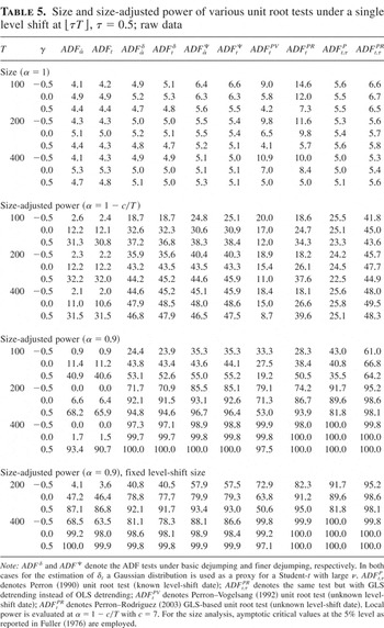
Results are reported in Table 5, where the first section contains simulated test sizes. The proposed tests have good size properties, comparable to the size of the tests assuming a known shift date, namely, ADFt.τP and ADFt.τPR. Conversely, because of the magnitude of the shift, the ADFtPV and ADFtPR tests are slightly oversized for γ = 0 and γ = −0.5. Regarding the (size-adjusted) power against local alternatives (second section of the table), we observe that in the presence of large shifts, the power of the proposed tests is above the power of the ADFtPR and the ADFtPV tests (the former being more powerful than the latter, as expected; cf. Perron and Rodriguez, 2003), in particular for larger sample sizes (T = 200,400). Compared to tests assuming a known shift date, although the proposed tests dominate the Perron (1990) test,
20This result is expected because the Perron (1990) test is not based on an efficient dejumping procedure under local alternatives; cf. Perron and Rodriguez (2003).

and ADFtΨ, show better power than the tests based on the basic dejumping,

and ADFtδ, in particular for moderate sample sizes and γ < 0. Moreover, our “finer” method does quite well compared to unit root tests assuming a level shift at an unknown date and, for samples of at least 200 observations, also with the tests assuming a known shift date. The results do not qualitatively differ when the fixed alternative α = 0.9 (third section of the table) is considered.
Size and size-adjusted power of various unit root tests under a single level shift at [lfloor ]τT[rfloor ], τ = 0.5; raw data

We conclude with a discussion of the fixed alternative α = 0.9 when the size of the single level shift is kept constant at four times the standard deviation of the innovations, corresponding to (16) with T = 100. Results for T = 200,400 are reported in the fourth section of Table 5. Under a fixed alternative and fixed level-shift size, as the sample size gets larger our tests tend to be outperformed by some of the existing tests, in particular for γ ≤ 0. For γ > 0, the proposed tests do better than the ADFtP test, and for γ = 0.5 they are comparable with the ADFtPR test, which, however, does better for γ ≤ 0. Notice that here the effect of the (fixed) level shift on the power of standard ADF tests becomes negligible as the sample size grows.
6. FURTHER ISSUES
In this section we briefly show how the proposed tests can be used in the case of a linear time trend and in the case of unknown autoregressive order.
6.1. Linear Time Trends
Although all the analytical results given so far are derived under the assumption of no deterministics in the DGP, in the presence of linear time trends the proposed tests can be successfully applied in conjunction with a proper detrending procedure.
The approach we suggest is to combine pseudo-GLS detrending (see Elliott, Rothenberg, and Stock, 1996) with dejumping in the computation of the ADFδ and ADFΨ statistics.21
Given a time series Xt, the pseudo-GLS detrended series at α := 1 − c/T (c ≥ 0) is defined as

, where (X0α,Xtα) := (X0,(1 − αL)Xt), (Z0α,Ztα) := (Z0,(1 − αL)Zt), and

minimizes

.
(1) δt is estimated using basic dejumping (i.e., neglecting the presence of the linear trend);
(2) level shifts are removed by computing

as in Section 3.1;
(3) pseudo-GLS detrending is applied to

;
(4) the ADFδ statistics are obtained from an ADF regression for the detrended

.
As in Section 4, via an iterative procedure it is also possible to obtain the estimates of the level-shift indicators jointly with those of the autoregressive coefficients and the coefficients of the linear trend Zt = (1,t)′. To this end, the vector ξ and the mapping ΨT of Section 4 are augmented with components φ = (φ1,φτ)′ and ΨTφ = (ΨT1,ΨTτ)′ for the coefficients of the linear trend. In place of etd, the estimates etd,τ := etd − φτ of εt + δtθt are used in the definition of ΨTtδ and ΨTλ. The updated dejumped series is now

; it is GLS-detrended to get XtΨ,τ and the updated estimate ΨTφ. ADF regression is performed on XtΨ,τ instead of XtΨ, and etΨ are replaced by etΨ,τ := etΨ − ΨTτ. The iteration is initialized with the outcome of the basic dejumping procedure, see the preceding steps 1–4.
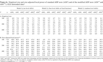
As is standard, we evaluate the properties of the tests using pseudo-GLS detrending at α := 1 − c/T, with c = 13.5. Results are reported in Table 6A (size) and Table 6B (local power). All conclusions obtained for the case of no deterministic terms carry over: first, in the absence of level shifts our tests behave as the standard ADF tests, whereas in the presence of shifts our tests do not experience the serious power loss of standard ADF tests. The only difference from the results in Table 1 is that in the presence of shifts the (still severe) power loss of standard ADF tests is partially mitigated by detrending the data.22
Further simulations (not reported) have shown that OLS detrending could be used instead of pseudo-GLS detrending. Obviously, OLS detrending leads to different (asymptotic) power properties (cf. Elliott et al., 1996; Müller and Elliott, 2003).
Empirical size and size-adjusted local power of standard ADF tests (ADF) and of the modified ADF tests (ADFδ and ADFΨ); GLS detrended data*

6.2. Unknown Autoregressive Order
So far, we have assumed that the autoregressive order k of the errors is known to the econometrician. In more realistic situations, k is unknown and needs to be estimated.
To deal with unknown lag order we suggest the following strategy, which combines our test procedure with standard methods for the determination of the lag order. In the first round, the basic dejumping algorithm of Section 3 (which does not require specifying k) is applied, and the dejumped time series,

, is obtained; see steps 1 and 2 in Section 3.1. In the second round, using

, a standard criterion for the determination of the lag order is employed; this delivers an estimate of k, say,

. In the final round, the ADFδ statistics are computed (see step 3 in Section 3.1) fixing the number of lags at

.
Tests based on the finer dejumping of Section 4 can be implemented also: once k has been estimated as described previously, ADFΨ statistics can be constructed by fixing k at

.
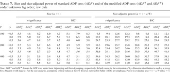
In Table 7 we report the results from a small Monte Carlo experiment based on model S4 (four level shifts at fixed relative locations). Two criteria for lag order determination are used: a sequential t-test and the Bayesian information criterion (BIC); see Ng and Perron (1995). The size of the tests is largely acceptable, with the tests based on the sequential t-tests being slightly more liberal than the tests based on the BIC. Also, ADFΨ tests are slightly oversized when compared with the basic tests ADFδ. The (local) power of the tests is not too distant from the power obtained by fixing k at its true value. Again, the joint estimation procedure of Section 4 leads to better power for negative values of γ.
Size and size-adjusted power of standard ADF tests (ADF) and of the modified ADF tests (ADFδ and ADFΨ) under unknown lag order; raw data

7. CONCLUSIONS
We have proposed a modification of the well-known augmented Dickey–Fuller (ADF) tests that allows testing for unit roots in the presence of multiple level shifts. Differently from existing work, we do not restrict the number of level shifts—which occur at random dates and have random sizes—apart from requiring it to be bounded in probability. The proposed tests have a limiting null distribution for which critical values are well known; moreover, they have the same asymptotic power functions as standard ADF tests under no level shifts. A Monte Carlo simulation has shown that the new tests behave well in finite samples and that they can account for linear time trends and unknown lag orders.
The results of the paper can be extended in various directions, which we reserve for further research. For instance, the finite autoregression assumption may be replaced by a general linear process assumption, along the work of Chang and Park (2002). A further important extension is to cointegrated models.
APPENDIX A: Mathematical Appendix
The Appendix contains proofs of the results given so far. The following notation is used: as previously, P denotes the sequence of probability measures induced by model (1), conditionally on NT ≥ 1 and under Assumptions

and

. Under the hypotheses

and

(null and local alternatives), the measure P specializes to Pc (c ≥ 0), whereas under

(fixed stable alternative), P specializes to Pf. For a sequence {yt} of random variables, maxt≤T{yt} := max−k≤t≤T{yt}, maxt:δt=1{yt} := max1≤t≤T{δt yt}, and mint:δt=1{yt} := (maxt:δt=1{yt−1})−1. An asterisk denotes true parameter values in cases of ambiguity.
A.1. Preliminary Lemmas.
LEMMA A.1. The following magnitude orders hold:
(i) maxt≤T|Yt| = OPc(T1/2);
(ii) if maxt≤T|εt| = OP(Tτ), τ ≥ 0, then maxt≤T|ut| = OP(Tτ), maxt≤T|Yt| = OPf(Tτ), and maxt≤T|ΔYt| = OP(Tτ);
(iii) if EP|ε1|ν+1 < ∞, ν ≥ 0, then

.
Proof. As εt, Y−k−1, and (u−2k,…,u−k−1) are assumed independent of δs for all t and s, conditioning on NT ≥ 1 in the definition of P is irrelevant for this proof. Under Pc we have that

(see (2) for the definition of Bc); hence (i). In (ii) the evaluation of maxt≤T|ut| (and under Pf, also those of maxt≤T|Yt| and maxt≤T|ΔYt|) holds since ut (resp. Yt and ΔYt) has a moving average representation with exponentially decreasing coefficients. Under Pc, from ΔYt = (−c/T)Yt−1 + ut and (i) it follows that maxt≤T|ΔYt| inherits the magnitude order of maxt≤T|ut|.
As to part (iii), because ut is the stationary solution of

, (ut)ν+1 is stationary and ergodic by Theorem 3.35 of White (2001). Then EP|ε1|ν+1 < ∞ implies, by the Marcinkiewicz–Zygmund inequality, that EP|ut|ν+1 < ∞. By an ergodic law of large numbers (LLN) (White, 2001, Thm. 3.34),

. Under Pf a similar argument applies to

. Under Pc, the evaluation

follows from the inequalities

and

; see (i). █
LEMMA A.2. If yt = OP(1) is a sequence of random variables independent of δs for all t,s under P, then

and maxt:δt=1|yt| = OP(1).
Proof. This is direct from the definitions of the measure P (by Assumption

) and of boundedness in probability. █
A.2. Proof of Theorem 1 and Related Results.
To avoid confusion with the conditional measure P, we use Q for the measure in Theorem 1.
A.2.1. Proof of Theorem 1 (Part I).
Here we derive the weak limit of the process T−1/2X[lfloor ]T·[rfloor ]. The limiting distributions of the ADF statistics will be obtained at the end of Section A.2.2.
Recall that Xt = Yt + μt and define

. To obtain the weak limit of T−1/2μ[lfloor ]T·[rfloor ], we start from the convergence of

and then use the representation

.
First, we show that the serial dependence of {ηt*} is lost in the limit of μ[lfloor ]T·[rfloor ]*. Consider, possibly upon enlarging the underlying probability space, a doubly infinite matrix

of i.i.d. random variables, with ω1t := ωt, and which is independent of {δt}t=1T and {Yt}t=−k−1T. Denote by rt the time of the last shift occurrence before time t (rt := −∞ if there are no shifts before time t) and for t = 1,…,T define

where

. For a fixed T the vector {ηt+}t=1T is distributed as T independent draws from the distribution of η1* (no ωit is present in two different ηt+'s) and is independent of {δt}t=1T (direct by writing its distribution conditional on {δt}t=1T and observing that it does not depend on {δt}t=1T). Thus, the weak limit of

obtains from Theorem 3.1 of Leipus and Viano (2003). Because E|ηt+| = E|η1*| < ∞ (as implied by E|ωt,i| = E|ω1| < ∞ and

, we have that

in

, where

is the Poisson process defined in Theorem 1.
Next, we argue that also μ[lfloor ]T·[rfloor ]* has

as its weak limit. For s ∈ [0,1] we have that

By the independence of ω's and δ's, and with mT := min1≤t≤T{t − rt} denoting the minimum distance between two consecutive shift dates (∞ if at most one shift occurs),

Because

by assumption and

, it follows that

and, further, that

by dominated convergence. Thus, by taking expectations in the preceding display,

because ENT2 → G(1) + G(1)2 by a direct calculation (G denoting the Poisson intensity), so that maxs∈[0,1]|ϑs| = oQ(1) by Markov's inequality.
The last relation is equivalent to

, and hence μ[lfloor ]T·[rfloor ]* has the same weak limit as

in

. Because of the equality

, the convergence

is expected. For brevity and consistency with further references, we note that it follows, e.g., from Theorem 2.7 of Kurtz and Protter (1991). On the other hand, using standard local-to-unity asymptotics,

in

. Because of the stochastic independence of μt and Yt, the joint convergence

in the product space

obtains. The map (x,y) [map ] x + y is continuous on the support

of

, and therefore,

by the continuous mapping theorem (CMT).
Note next that (1) implies the following representation of ΔXt:

Let ∇Xt−1 := (ΔXt−1,…,ΔXt−k)′ and similarly for ∇Yt−1 and ∇μt−1. The numerator of the

statistic based on Xt can be expressed as

, where

see Chang and Park (2002). We write the limits of these and of related quantities using stochastic integrals. The limits follow from Theorem 2.7 of Kurtz and Protter (1991), in view of the relation NT = OQ(1) and of the convergence

on the space

of 5 × 1-vector càdlàg functions, endowed with the Skorohod topology. Convergence (A.2) holds on the product space

similarly to (A.1) and can be extended to

by Proposition VI.2.2(b) of Jacod and Shiryaev (2003). Thus, Kurtz and Protter's theorem delivers that, jointly with (A.2),

Another useful limit is that of

and its continuous transformations. As (i)

for i ≠ j, (ii) δT−i = 0 with probability approaching one for i = 0,…,k, and (iii) maxt:δt=1|ηt| = OQ(1) by Lemma A.2, it holds that

the limit as

by (A.2), (A.3), and the CMT. Convergence is joint with (A.2) and (A.3) again by the CMT. █
A.2.2. Proof of Theorem 1 (Part II).
To complete the proof of Theorem 1, we need the following lemma.
LEMMA A.3. Let Ω∇∇ denote the probability limit of

and let Ω1∇ be the nonrandom vector defined through

(see, e.g., Hansen, 1992; Phillips, 1987, Lem. 1), where 1k is a k × 1 vector of ones. Then, as T → ∞, the following converge jointly:
(i)

;
(ii)

;
(iii)

;
(iv)

;
(v)

;
(vi)

.
Proof. Convergence (i) obtains from (6) and the CMT. Further, the left side of (ii) equals A1 + A2 + A3, with the following Ai's. First,

by (A.3) and the CMT, because σ = σε/Γ(1). Second,

, which can be written, with γ0 := −1, as

The first summation in brackets contributes to A2 with

. The contribution of the second summation is a continuous transformation of M in (A.4) and tends to

. Because

by Lemma A.2, we can conclude that

. Third,

by (A.2) and the CMT. Combining the limits of the Ai's, and recalling that Bc(s) satisfies dBc(s) = −cBc(s) ds + dB(s), gives the limit in (ii).
With

, convergence (iii) follows from the identity

Here B = oQ(1) by Lemma A.2 applied elementwise, whereas the other two terms have limits Ω∇∇ and

, respectively, the latter by (A.4). For (iv), note that

where the limit of the first term on the right side is given in the hypothesis, the second term equals

by Lemma A.2 and converges weakly to

by partial summation and (A.3), and, again by Lemma A.2, the third term equals

and can be seen to tend to

by (A.3), (A.4), and the CMT.
For items (v) and (vi) we have

because two kinds of oQ(1) terms appear in these expressions. First,

,

, and

are oQ(1) by Lemma A.2. Second,

by an LLN for

and by (A.3) for

, and similarly for F and H, which contain overnormalized contributions of cT−1Yt−1. The terms with nonzero limits are

by an LLN,

by (A.4) and the CMT, and

by (A.4) and the CMT again.
Convergence is joint because, up to terms with constant probability limits, the left sides (i)–(vi) can be collected in a continuous transformation of the left sides of (A.2) and (A.3). █
Let

and

, which can be written more shortly as

and

. It follows from Lemma A.3 that

Because

, it follows that

, and hence,

From Lemma A.3 we find that

. Together with

, these results yield the limit of

in (7) with

. We have used that Γ∞ > 0 since, for each outcome in the sample space, it is the value at unity of the characteristic polynomial of a stationary AR(k) process with covariance of order i = 0,…,k equal to

; cf. Prob. 1.3 in Brockwell and Davis (1991).
The proof for the t-statistic is similar. Specifically, as AT2/T2 = OQ(1) (see the preceding discussion), the following equalities hold:

with (Chang and Park, 2002)

From Lemma A.3 it obtains, after rearranging terms, that

. Hence, (A.5) and (A.6) ensure that

which is the limit in (7) with ϰ1 := C∞Γ∞−2σ−2. In the special case k = 0, we have Γ∞ = 1,

, and σ2 = σε2, from where the simpler expressions for ϰ0 and ϰ1. █
A.3. Proof of Theorem 3 and Related Results.
A.3.1. Uniform Evaluations Related to Dejumping.
LEMMA A.4. Suppose that

is a sequence of random variables such that

. Then

and

is bounded away from zero in P-probability.
Proof. Recall that θt = T1/2ηt. The evaluation of

follows from the inequality

by applying Lemma A.2 to the first two maxima on the right side and the hypothesis of the lemma to the last one. The fact that

is bounded away from zero in P-probability obtains from

. The first minimum on the right side equals (maxt:δt=1 ηt−2)−1 = (OP(1))−1 by Lemma A.2 and the assumption that ηt−1 = OP(1), whereas the second one is 1 + oP(1). Indeed, because

it follows that, with P-probability approaching one,

Remark A.1. In the discussion of joint dejumping and parameter estimation, instead of a sequence of random variables

, a sequence of random functions

of a vector variable with domain

(say) will appear. If we suppose that

, the conclusions of Lemma A.4 hold for

and

. The proof carries over with only notational changes.
The next lemma provides conditions for uniformly consistent detection of level shifts.
LEMMA A.5. Let

and ζ(·) be as in Lemma 1,

be as in Lemma A.4, and

be as in (10). Then

and

, provided that

.
Proof. Recall that for functions f with appropriate domain we write

for

and similarly for suprema involving the components of ζ = (ζλ,ζη,ζσ)′. As φν(e;a2) of (10) equals a−1(1 + e2/(νa2))−(ν+1)/2 up to a multiplicative constant, and 0 < ζλ < T on

with P-probability tending to one, we find that

Let

and

. As

, it follows that

Summing over t, and accounting for the assumption that NT = OP(1), yields the evaluation

Because

and, by Lemma A.4,

is bounded away from zero in P-probability, we have that

uniformly on

. Further,

again by Lemma A.4, and as

is bounded away from zero in P-probability, it follows that MT,2 ≤ OP(1) uniformly on

. Combining the two conclusions yields

.
The magnitude order of

is addressed next. By evaluating from below the denominator of (10), it can be concluded that

The contribution of the factors not containing

is OP(T−3/2) uniformly on

, whereas the last factor does not exceed unity. Further, by applying to

the inequality (1 + x2)(ν+1)/2 < 2(ν+1)/2(1 + |x|ν+1), it is seen that

, because

. Hence,

Provided that

, we get that

uniformly on

. This result and the first part of the lemma give

on

, again uniformly. █
Remark A.2. If

are random functions satisfying the condition of Remark A.1, and if also

, then the conclusions of Lemma A.5 hold for

and

. Again, the proof is only notationally more involved.
Next, let d = (d1,…,dT)′ be a (continuous)

-valued random function with domain

(say). For instance, in the proof of Lemma 1 later in this Appendix, d will have components

and domain

. In the next lemma we consider as a function on

the dejumped series

and, among other things, evaluate the distance between {Yt} and {Xtd} depending on how close d is to δ = (δ1,…,δT)′. The notation

is used.
LEMMA A.6. Let maxt≤T|εt| = OP(Tτ), τ ≥ 0. If d is defined on a set

such that

for some β ∈ [0,τ), with β + τ < ½, then
(i)

and

;
(ii)

,

with aT = OP(Tβ) and bT = OP(Tβ+τ−1/2), and

;
(iii)

with

and

,

, and

;
(iv)

,

, and if, additionally,

, then

, where

.
Proof. For t = 1,…,T we have

, and for such t we find


and for t = −k,…,0, Xtd − Yt = 0. The first relation in (i) follows using (A.8):

with magnitude orders from Lemmas A.2 and A.1(ii) and from the hypothesis. Together with maxt≤T|Yt| = OPc(T1/2) (= OPf(Tτ)), (A.10) implies the other relations in (i).
The right side of (A.10) is a uniform upper bound for

(see equation (A.9)), hence, the first relation in (ii). Again from (A.9), |ΔXtd − ΔYt| for t = 1,…,T does not exceed

from where, upon taking suprema, the definitions of aT and bT in (ii) are obvious. Their magnitude orders follow as in (i). Further,

by the preceding evaluation, Lemma A.1(ii), and the inequality β < τ.
A vector version

obtains readily and, together with (i), gives for Yt := (Yt,(∇Yt)′)′ and Xtd := (Xtd,(∇Xtd)′)′ the first relation in (iii). As max0≤t≤T∥DTYt∥ ≤ maxt≤T|T−1/2Yt| + k maxt≤T|ΔYt| = OP(Tτ), it holds further that

which is OP(Tτ) for β < τ. Similarly, maxt≤T|Yt| = OPf(Tτ) leads to max0≤t≤T∥Yt∥ = OPf(Tτ) and

.
For part (iv), note that

, so that

by the weak convergence of

under Pf and by Lemma A.1(ii). Using (A.8), we find the decomposition

, where, first,

satisfies

by Assumption

, Lemma A.2, and (A.11). Second, as

on

, we see that

satisfies

and similarly,

satisfies

using Lemma A.1(ii) and again (A.11). The first relation in (iv) follows by combining the preceding magnitude orders. The second relation obtains upon partial summation; with

, so that

, we find that

uniformly on

by (i) and (ii). Finally,

as shown earlier, whereas, using (A.8), we can see that

because

,

using Lemma A.2 and the assumed magnitude orders of

and

, whereas the magnitude orders of cross-products in the expansion of (Xtd − Yt)2, summed over t, follow from the preceding three evaluations and the Cauchy–Schwartz inequality. █
We conclude Section A.3.1 with an important lemma on the properties of OLS estimators in the ADF regression based on Xtd, with Xtd as in Lemma A.6.
LEMMA A.7. Let

and

be the OLS estimators from the regressions Xtd = (α,γ′)Xt−1d + errort and Yt = (α,γ′)Yt−1 + errort, and let

and

be the respective residual variances. Under the assumptions of Lemma A.6, with β = 0 and τ < ½, it holds that
(i)

.
Furthermore, if additionally

, then
(ii)

and

where (α*,γ*′) under

is defined through the representation Yt = (α*,γ*′)Yt−1 + εt implied by (1),

, and i := (1,01×k)′.
Proof. To prepare jointly the proof of (i) and (ii), we define (α*,γ*′) := (1,γ*′) under

and

, and c* := 0 under

and

. With this notation,

where

and

. The representation of ΔXtd obtains by inserting ΔYt = ΔXtd + (ΔYt − ΔXtd) and Yt−1 = Xt−1d + (Yt−1 − Xt−1d) into that of ΔYt.
Define DT := DT, BT := diag(T,T1/2), h := ½ under

and

, and DT := Ik+1, BT := I2, h := 1 under

. With

,

,

,

, and

, we have


We show that

, j ∈ {1,e,∇}, are OPc(Tτ−1/2) and that

, and

are OPf(Tτ−1/2). Then we use the standard facts that, under P, S11T has a positive definite and S1eT has a finite (zero, under Pf) weak limit.
First,

under

and

, where the maxima are OPc(Tτ) and the summation is bounded by

, all uniformly on

; see Lemmas A.1(ii) and A.6 (with β = 0). Hence, r11T = OPc(Tτ−1/2). Under

, we have the following uniform evaluations on

equals

by Lemmas A.1(ii) and A.6(iii) and (iv), applied in this order;

equals

by Lemma A.6(iii) and (iv), and

equals

by Lemma A.6(i) and (ii). From the last three evaluations,

on

, and from Lemma A.6(iv),

under the assumption that

.
Second,

, where

by partial summation. Therefore,

is bounded by

on

, because the factor in parentheses is OP(1) by Lemma A.6(i) and (ii), and

with U = OP(1) denoting a contribution from initial values. Still by Lemma A.6(ii), and because

, we find that

uniformly on

. By combining the preceding evaluations,

.
An evaluation of

can be obtained similarly:

which is OP(Tτ) by Lemma A.6. Under

and

this shows that

. Under

, it gives together with Lemma A.6(iv) that

.
We proceed with the proof of (i). From (A.12), (A.13), and the identity (S11T + R11T)−1 = (S11T)−1 − (S11T + R11T)−1R11T(S11T)−1 it follows that

equals

To evaluate this matrix, define the event

. As r11T = OPc(Tτ−1/2) and S11T converges weakly to an a.s. positive definite matrix under Pc, it holds that

, and it suffices to study outcomes in

. For such outcomes ∥(S11T + R11T)−1∥ ≤ ∥(S11T)−1∥(1 − ∥R11T∥∥(S11T)−1∥)−1 (this follows from ∥(S11T + R11T)−1∥ = ∥(S11T)−1 − (S11T + R11T)−1R11T(S11T)−1∥ ≤ ∥(S11T)−1∥ + ∥(S11T + R11T)−1∥∥R11T∥∥(S11T)−1∥ by solving the inequality for ∥(S11T + R11T)−1∥), so that

is dominated by

which is OPc(Tτ−1/2) by the first part of the proof and because (S11T)−1 and S1eT are OPc(1). With regard to residual variances,

As

uniformly on

(see Lemmas A.1 and A.6(ii)), and because

is a well-known fact, from the previous argument it follows that

. This completes the proof of (i).
Next, the identity (S11T + R11T)−1 = [Ik+1 − (S11T + R11T)−1(R11T − ii′ϒT)](S11T + ii′ϒT)−1 and (A.13) yield

, where

Using that ∥(S11T + ii′ϒT)−1∥ ≤ ∥(S11T)−1∥, we find that

does not exceed

as S11T converges to a positive definite matrix in Pf-probability, S1eT = OPf(T−1/2) by a central limit theorem, and the suprema were found to be OPf(Tτ−1/2). Further, for outcomes in the set

, with

, we have

so that

is bounded by OPf(1) times

similarly to

. This proves the first part of (ii). Because

can be written as

it is not hard to see that

, where, with

,

As

and

, we conclude that

. █
A.3.2. Proof of Lemma 1.
We check that, for 3 ≤ ν ≤ r − 1,

satisfies the hypotheses of Lemmas A.4 and A.5. First, maxt≤T|εt| = OP(Tτ) with τ = r−1 ≤ ¼ in view of Assumption

, and maxt≤T|ΔYt| = OP(Tτ) by Lemma A.1(ii). Hence, max1≤t≤T|ΔXt − εt − δtθt| = max1≤t≤T|ΔYt − εt| = oP(T1/2) as required in Lemma A.4 for

(from here and Lemma A.2, it is seen that max1≤t≤T|ΔXt| = OP(T1/2), which will be used subsequently). Second, (1 − δt)|ΔXt|ν+1 = (1 − δt)|ΔYt|ν+1 and

by Lemma A.1(iii), because ν + 1 ≤ r, and hence also Lemma A.5 is applicable to

. Recalling that

, from Lemma A.5 we obtain Lemma 1(i).
To prove (ii), we use (i) jointly with max1≤t≤T|ΔXt| = OP(T1/2):

uniformly on

. As (1 − δt)(ΔXt)2 = (1 − δt)(ΔYt)2 and δt ΔXt = δt(ΔYt + T1/2ηt), we can insert

in the preceding display. Combining the result with the relation

, which is direct from (i), we obtain (ii).
Part (i) and Lemma A.7 with

and

, t = 1,…,T, imply (iii).
Consider now the Jacobian

, where

and wt := (T,(ΔXt)2,−(ΔXt)2)′. It can be evaluated as follows:

We discuss the factors on the right side separately, starting from vt. First,

where

. A similar expression (with a different

) obtains for ∂[ln φν(ΔXt;ςσ)]/∂ςσ. Using that

, it follows that

Upon evaluation at (ςη,ςσ) = (ζη(z),ζσ(z)), all right sides in (A.15) are OP(1) uniformly on

. Also

. Hence,

. The other terms on the right side of (A.14) are max1≤t≤T∥T−1wt∥ ≤ 1 + 2T−1 max1≤t≤T(ΔXt)2 = OP(1) (see paragraph one of the proof) and

, which upon evaluation at ζ(z) is OP(T−1/2) uniformly on

(see part (i)). Part (iv) follows by inserting the obtained orders of magnitude into (A.14). █
A.3.3. Proof of Theorem 2.
(i) Existence. To be able to use a standard fixed-point theorem, we set up an auxiliary fixed-point problem for a self-map of a compact. For the auxiliary map, defined by centering, normalizing, and truncating ΦT, existence of a random fixed point is classical, and this point turns out to be a fixed point of ΦT, with P-probability tending to one.
Let

,

,

, and

. With

acting on z = (zλ,zη,zσ)′ according to ζ(z) = (zλ + NT,HT zη,zσ)′, let ΘT := ζ−1 ○ ΦT ○ ζ. As HT ≠ 0 P-a.s., ΘT is well-defined P-a.s. Further, let

be defined componentwise: for v ∈ {λ,η,σ}, (ΘTtr)v(z) := ΘTv(z) if

,

if

, and

if

. As ΘTtr is continuous and

is a convex compact, ΘTtr admits a random fixed point

. This is guaranteed by Theorem 10 in Bharucha-Reid (1976).
For outcomes such that

, we have zT = ΘTtr(zT) = ΘT(zT), i.e., ζT = ζ(zT) is a fixed point of ΦT. Because, in view of Lemma 1(ii), ΘT(zT) = ζ−1((NT,HT,σY2)′ + oP(1)) = (0,1,σY2)′ + oP(1), and because (0,1,σY2)′ is an interior point of

, it follows that

. Hence, ζT is a random fixed point of ΦT with P-probability approaching one, and by the choice of

, ζT is bounded and bounded away from zero in P-probability.
(ii) Uniqueness. We use a contraction argument. Let ςT have the properties of ζT from the existence part of the theorem. Fix ε > 0. Because NT, HT (by Lemma A.2 for ηt and ηt−1), ζT and ςT are bounded and bounded away from zero in P-probability, there exist constants qh > 2ql > 0 and a set

with

such that, for outcomes in

, NT ≤ qh, 2ql ≤ HT ≤ qh, ql13 ≤ ζT ≤ qh13, and ql13 ≤ ςT ≤ qh13, where the inequalities for ζT and ςT are componentwise. Define the compact

. Then, for outcomes in

, first,

, and second, the point (NT,HT,σY2)′ is interior for

and at a distance from the boundary of

bounded from below by a positive constant. From the latter and Lemma 1(ii), with

in place of

and with ζ(·) equal to the identity function, it follows that on some

, with

, and for T > T2 (say),

. By Lemma 1(iv), there exist T3 > T2 and

, with

, such that for T > T3 and on

,

. Because (ΦT)z′ is of dimension 3 × 3, under the same conditions,

, where the ith row of (ΦT)z′ is evaluated at zi (i = 1,2,3). By the mean-value theorem for ΦT on

, we see that for outcomes in

and for large T, ΦT is a contraction on

and has a unique (per outcome) fixed point on

by Banach's fixed-point theorem.
Consider finally T4 and

, with

, such that for T > T4 and outcomes in

, ΦT(ζT) = ζT and ΦT(ςT) = ςT. This is possible by the choice of ζT and ςT. Then, for outcomes in

and T > max(T3,T4),

and

must be equal to the unique fixed point of ΦT on

. Because

and ε is arbitrary, P(ζT = ςT) → 1.
(iii) Computability. A contraction argument is used again. Let

. As in the proof of uniqueness, on some event

, with

, and for T > T1 (say), ΦT is a contraction of

onto

, and

. Further, from the proof of existence, ΦT(ζT) = ζT on some

with

and for T > T5 (say). By Banach's fixed-point theorem, for T > max(T1,T5) and outcomes in

, with

, the sequence of iterates of ΦT converges to the unique (per outcome) fixed point ζT of ΦT on

.
(iv) Consistency. This part of Theorem 2 follows from Lemma 1(i) and (ii) by evaluating the functions there at

, with zT, ζ(·), and

as in the proof of existence. █
A.3.4. Proof of Theorem 3.
Under

and

, the result for

is direct from (2) and Lemma 1(iii), with the functions there evaluated at

and with ζ(·) and zT as in the proof of existence in Theorem 2. For ADFtδ, in addition to these results, also the conclusion that S11T + R11T(ζ(zT)) = S11T + oPc(1) is invoked to ensure asymptotic equivalence of the standard errors based on

and on Yt; see the proof and the notation of Lemma A.7.
Let the OLS estimators of α, γ, and σε2 from the ADF regression for

be

,

, and

and let ϑT := 1/(1 + ϒTi′(S11T)−1i) ∈ (0,1]. After some algebra, we obtain from Lemma A.7(ii) (upon evaluation of the functions there at zT, with dt(·) = δ(ΔXt;ζ(·)) and

) that, under the hypothesis

,

where S0∇∞ and S∇∇∞ are the Pf-probability limits, respectively, of

and

. Because, under

, α* = (α* − 1)Γ*(1) + 1 < 1 and ϒTi′(S11T)−1i = OPf(1), we find that

. Because

and (S11T + R11T(ζ(zT)))−1 = OPf(1) by Lemma A.7(ii) and its proof, it follows that

. Similarly, because

(see equation (A.16)), also

. █
A.4. Proof of Theorem 4 and Related Results.
Let ρ > 0 be a real number that we will choose as small as convenient. The compact

from the proof of Theorem 2 is replaced here by

, defined as

, with


A.4.1. More Lemmas.
The point at which ΨT is evaluated is specified as

, where

is the random function with components ξδ(xδ) = xδ + (δ1,…,δT)′, ξλ(xλ) = xλ + NT, ξη(xη) = HT xη and ξa,ξγ,ξσ are the identity functions, respectively, on

,

, and

. It will be shown that there exists a random sequence

such that Pc((ΨT ○ ξ)(xT) = ξ(xT)) → 1. The proof uses properties in the spirit of Lemma 1 that are worked out next. The argument of ξ and its components is subsumed; the notation

is employed for

and similarly for the components.
Upon substitution of d = (d1,…,dT)′ by ξδ in the definition of Xtd (t = 1,…,T), the dejumped series

obtains; we treat it, and also the associated residual series etξ := ΔXt − (ξa,(ξγ)′)DTXt−1ξ, as a function on

. Similarly, the updated dejumped series

and residuals etΨ := ΔXt − ΨTa,γ(ξ)DTXt−1Ψ are functions on

. Thus, so is

; see (10).
LEMMA A.8. If 3 ≤ ν ≤ r − 1, 2ρ(ν + 1) < 1, and maxt≤T|εt| = OPc(Tτ), then
(i)

and

;
(ii)

, with

as in Lemma A.7;
(iii)

and

;
(iv)

.
Proof. Without loss of generality, we take τ ≤ ¼, because E|ε1|4 < ∞ under Pc. Note also that ρ < ⅛ under the hypothesis of the lemma (this represents no restriction on the model).
For part (i), we check that Lemma A.5 (as stated in Remark A.2) is applicable to

. First, we evaluate etξ − εt − δtθt − (γ* − ξγ)′∇Yt−1 on

. Under

and

, they equal (−T−1c* − T−1/2ξa)Yt−1 − (ξa,(ξγ)′)DT(Xt−1ξ − Yt−1), where

,

, maxt≤T|Yt| = OPc(T1/2) and Lemma A.6(iii) with d(·) = ξδ(·),

, and β = ρ is applicable to

. By collecting the magnitude orders, we obtain that

where

. Thus, because

, max1≤t≤T∥∇Yt−1∥ = OPc(Tτ) by Lemma A.1(iii), δt ≤ k, and ρ + τ < ½, it follows that

, as required in Remarks A.1 and A.2.
Second, we verify that

. Indeed, in consequence of (A.17) and the inequalities ρ(ν + 1) < ½, ρ + τ < ½, it holds that

uniformly on

. Further, for ν + 1 ≤ r, we have E|εt|ν+1 < ∞, so that

and

by Lemma A.1(iii), whereas

and

. These imply the asserted uniform order of

. Having checked the conditions of Remark A.2, we obtain part (i).
Part (ii) follows from (i) and Lemma A.7(i) with d(·) = ΨTδ(ξ(·)),

. Further, (ii) together with the standard properties

and

implies that

,

, and

. These are useful in a derivation similar to that of (A.17) but this time invoking for

Lemma A.6(iii) with d(·) = ΨTδ(ξ(·)),

, and β = 0, the latter in view of (i):

because max1≤t≤T∥∇Yt−1∥ = OPc(Tτ) by Lemma A.1(ii). From here, Lemma A.2, and the assumption that maxt≤T|εt| = OPc(Tτ), (iii) follows.
Finally, part (iv) can be derived starting from

by (i) and (iii). Next, by applying to u = etΨ and v = εt + T1/2δtηt the inequality |u2 − v2| ≤ |u − v|2 + 2|u − v| |v|, and then (A.19) to evaluate |u − v|, we see that

Inserting

and combining with the previous display completes the proof of part (iv). █
Next, for use in contraction arguments, we evaluate the Jacobian matrix of ΨT. For a matrix A = (aij), introduce ∥A∥1 := [sum ]i,j|aij| and ∥A∥h := maxj [sum ]i|aij|.
LEMMA A.9. Let each row of the Jacobian matrix (ΨT)ς′ = (ΨT(ς))ς′ be evaluated at some point of the form ξ(x), with x possibly varying across rows, and let (ΨT)□′ denote the resulting matrix as a function on

. Suppose that Assumption

is satisfied for some r ≥ 5 and that 4 ≤ ν ≤ r − 1. Then there exists a ρ > 0 such that

.
Proof. The proof is rather long but mechanical and hence is omitted from brevity. It is available in the accompanying working paper, Cavaliere and Georgiev (2006), or from the Web page http://www2.stat.unibo.it/cavaliere/lshifts. █
A.4.2. Proof of Theorem 4.
The argument is similar to that for Theorem 2. For ξ(·) defined in Section A.4.1, let ΞT := ξ−1 ○ ΨT ○ ξ; it is well-defined Pc-a.s.
Let ρ > 0 be chosen such that the conclusions of Lemma A.8 are applicable; this choice is possible under the conditions of Theorem 2. Further, let

be obtained from ΞT by truncating it as follows: (ΞTtr)δ(x) := ΞTδ(x) if

and (ΞTtr)δ(x) := Tρ−1/2ΞTδ(x)/Σt=1T|ΞTtδ(x)| otherwise; (ΞTtr)γ(x) := ΞTγ(x) if

and (ΞTtr)γ(x) := γ* + (ΞTγ(x) − γ*)/∥ΞTγ(x) − γ*∥ otherwise; (ΞTtr)λ, (ΞTtr)a, (ΞTtr)η, (ΞTtr)σ are defined similarly to the components of ΘTtr in the proof of Theorem 2. Then ΞTtr has a random fixed point ϰT on

by Theorem 10 in Bharucha-Reid (1976). Define ξT := ξ(ϰT). Similarly to the proof of Theorem 2, but invoking Lemma A.8(i), (ii), and (iv) instead of Lemma 1, we conclude that Pc(ΨT(ξ(ϰT)) = ξ(ϰT)) → 1, i.e., ξT has property (i).
Because

, from Lemma A.8 it follows that ξT also has property (ii). Property (iii) follows once it is noticed that the ADF statistics based on the dejumped series are

and ADFtΨ = T−1/2ΨTa(ξT)[σΨ2(ξT)v11]−1/2, where σΨ2(ξT) is the residual variance from (13) and v11 is the first entry of the matrix

, both evaluated at ξT. As

, Lemma A.8 allows us to invoke Lemma A.7(i) and to obtain the limiting distributions of the statistics as in the proof of Theorem 3.
In what follows we assume that r ≥ 5, and we choose ρ such that Lemma A.9 is applicable.
To discuss uniqueness, fix an ε ∈ (0,½). Because

is convex, for every

, by the mean-value theorem ΞT(x1) − ΞT(x2) = (ΞT)□′(x1 − x2), where (ΞT)□′ is the Jacobian matrix (ΞT)x′ with each row evaluated at some point in

, possibly varying across rows and also with x1,x2. We have

in view of Assumption

and Lemmas A.2 and A.9, where (ΨT)□′ is as in Lemma A.9. Therefore, we can find a set

, with

, such that for T > T1 (say) and outcomes in

, ∥(ΞT)□′∥h ≤ ½ on

. Further,

; i.e., ΞT is Lipschitz on

with modulus ½. On the other hand, in view of Lemma A.8(i), (ii), and (iv), there exist a set

, with

, and an integer T2 ≥ T1 such that, on

and for T > T2,

. Thus, for T > T2 and outcomes in

, ΞT is a contraction on

, and by Banach's fixed-point theorem, ΞT has a unique (per outcome) fixed point on

.
Further, if ξT and ςT satisfy part (i), there exists a set

, with

, such that on

and for T > T3 (say), ΨT(ξT) = ξT and ΨT(ςT) = ςT. If they also satisfy parts (ii) and (iii), so that ΨT(ξT) = ξ(ϰ∞) + oPc(1) and ΨT(ςT) = ξ(κ∞) + oPc(1), with ϰ∞ := (0T+1,γ*′,0,1,σε*2)′ and with convergence rate faster than the shrinkage rates of

and

for the respective components ΨTδ(ξT),ΨTδ(ςT) and ΨTa(ξT),ΨTa(ςT), then on some set

with

, and for T > T4 ≥ T3 (say),

and

. On

and for T > T4, ξ−1(ξT) and ξ−1(ςT) are fixed points of ΞT on

, whereas on

with

and for T > max(T2,T4), we must have ξ−1(ξT) = ξ−1(ςT). As ε is arbitrary, uniqueness of ξT with Pc-probability tending to one follows.
Finally, consider computation. From the proofs of Theorems 2 and 3,

at a faster rate than the shrinkage rates of

and

for xT0δ and xT0a, respectively. Thus,

on some

with

and for T > T5 (say). By Banach's fixed-point theorem, on

and for T > max(T2,T5), the sequence defined by xTi := Ξ(xT,i−1), i ≥ 1, converges as i → ∞ to the unique (per outcome) fixed point of ΞT on

, which on

equals ξ−1(ξT). Because

, we obtain the convergence ξTi = ξ(xTi) → ξT as i → ∞ with Pc-probability tending to one as T → ∞. █