1. Introduction
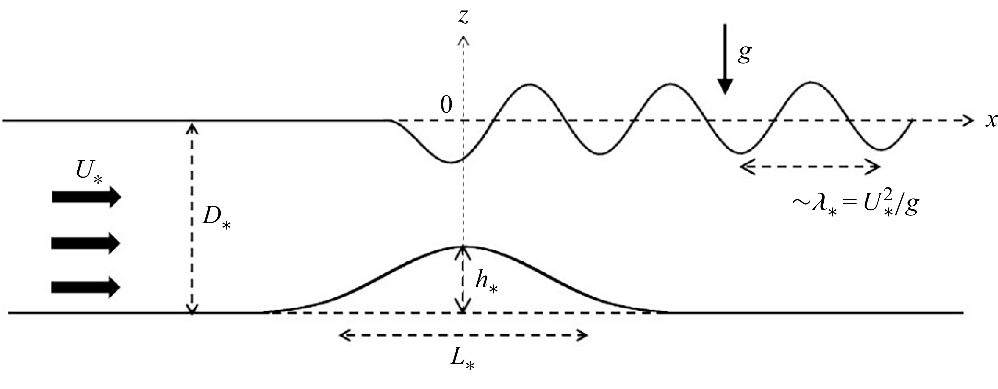
This paper revisits two-dimensional free-surface flow due to a uniform stream
 $U_{\ast }$
flowing over smooth, locally confined (width
 $L_{\ast }$
in the streamwise direction) topography of peak height
 $h_{\ast }$
(figure 1). Ignoring viscosity and surface tension, the flow is controlled by the dimensionless parameters
 \begin{align} \mu =\frac {\lambda _{\ast }}{L_{\ast }}, \qquad \varepsilon =\frac {h_{\ast }}{\lambda _{\ast }}, \qquad D=\frac {{D}_{\ast }}{\lambda _{\ast }}, \end{align}
where
 $\lambda _{\ast }=U^2_{\ast }/g$
is the gravity wavescale (
 $g$
is the gravitational acceleration) and
 $D_{\ast }$
is the (constant) undisturbed water depth far upstream. The depth parameter
 $D$
also specifies the Froude number
 \begin{align} F=\frac {U_{\ast }}{(gD_{\ast })^{1/2}}=\frac {1}{D^{1/2}}. \end{align}
Flow schematic.

Using potential flow theory, the classical analytical treatment (e.g. Stoker Reference Stoker1957) assumes that the topography has infinitesimal height (
 $\varepsilon \rightarrow 0$
). The boundary conditions on the free surface and the topography then are linearized about the undisturbed stream over a flat bottom and the problem is solved by transforms. This linear solution approaches a steady state that features a radiating gravity wave train downstream if the flow is subcritical (
 $F \lt 1$
) but remains localized over the topography if the flow is supercritical (
 $F \gt 1$
). At
 $F=1$
, the linear steady-state response breaks down due to a resonance phenomenon. As a result, for
 $F \approx 1$
nonlinearity cannot be neglected, and the response exhibits periodic shedding of solitary waves upstream (Akylas Reference Akylas1984; Cole Reference Cole1985).
A complementary theoretical approach is based on the nonlinear shallow-water equations, which formally approximate the full potential flow equations in the limit
 $\mu \rightarrow 0$
with
 $\varepsilon = O(1)$
. This so-called ‘hydraulic’ theory is expected to be valid for topography of large horizontal extent and finite height. Due to the assumption
 $\mu \rightarrow 0$
, the hydraulic approximation neglects dispersion altogether and cannot account for steady radiating waves. On the other hand, it has been used to study the formation of hydraulic jumps and related phenomena due to finite-height topography, which are beyond the reach of linear theory (see Baines (Reference Baines1995) for a comprehensive review).
The focus here is on steady, subcritical flow over extended, finite-height topography
 \begin{align} F \lt 1\ \ (D \gt 1), \qquad \mu \ll 1, \qquad \varepsilon = O(1). \end{align}
For
 $F\lt 1$
, the nonlinear shallow-water theory predicts a steady state only if the topography peak height is below a critical value,
 $\varepsilon \lt \varepsilon _{\textit{crit}}(F)$
. The associated free-surface disturbance is localized in the vicinity of the topography. When
 $\varepsilon \gt \varepsilon _{\textit{crit}}$
, the flow is partially blocked by the topography and hydraulic jumps form upstream and downstream (Long Reference Long1954; Houghton & Kasahara Reference Houghton and Kasahara1968). These two types of hydraulic states also were confirmed by laboratory experiments (Long Reference Long1954, Reference Long1970).
In recent related theoretical work, (Kataoka & Akylas (Reference Kataoka and Akylas2024), hereafter referred to as KA2024) studied asymptotically the effects of small dispersion (
 $0 \lt \mu \ll 1$
) on steady subcritical free-surface flow (
 $F\lt 1$
) over smooth topography of small but finite height (
 $0\lt \varepsilon \ll 1$
). As noted above, when
 $F\lt 1$
, dispersion is responsible for the appearance of a steady radiating gravity wave train downstream. Remarkably, in the weakly nonlinear–weakly dispersive limit,
 $\mu , \varepsilon \ll 1$
, the amplitude of this wave, although formally exponentially small with respect to
 $\mu$
, hinges on a nonlinear mechanism. Furthermore, comparisons of asymptotic results with numerical solutions of the full water-wave equations suggest that this mechanism controls the wave response for a broad range of flow conditions, in sharp contrast to the classical linear theory which has very limited validity.
In light of these findings, it is natural to wonder about the effects of weak dispersion (
 $0 \lt \mu \ll 1$
) in the nonlinear locally confined steady state predicted by hydraulic theory for subcritical flow (
 $F \lt 1$
) over topography of finite
 $\varepsilon \lt \varepsilon _{\textit{crit}} (F)$
. This issue is addressed here by developing an asymptotic theory in the limit
 $\mu \ll 1$
for the downstream wave response due to smooth, symmetric topography of
 $O(1)$
height. Similar to KA2024, the wave amplitude
 $R$
is exponentially small with respect to
 $\mu$
,
 $R = O (\exp (-q/\mu ) )$
. However, rather than a constant set by the linear solution, here the (positive) exponent
 $q$
is found to be a decreasing function of
 $\varepsilon$
with
 $q \rightarrow 0$
as
 $\varepsilon \rightarrow \varepsilon _{\textit{crit}}$
. Thus, increasing the topography height boosts the radiating wave. Moreover, for
 $\varepsilon$
near the critical topography height
 $\varepsilon _{\textit{crit}}$
, this (formally exponentially small) wave approaches the same level as the hydraulic disturbance over the topography. As a result, the nonlinear shallow-water equations are expected to break down in the vicinity of
 $\varepsilon _{\textit{crit}}$
, however small
 $\mu$
may be.
The asymptotic results for the radiating wave amplitude and phase are confirmed by numerical solutions of the full steady water-wave equations for topography with a sech profile. These computations also indicate the existence of a limiting topography height,
 $\varepsilon _{\textit{lim}}$
, close to
 $\varepsilon _{\textit{crit}}$
depending on
 $F$
and
 $\mu$
, above which a steady solution that approaches the uniform stream far upstream and remains finite downstream, is not possible. For
 $\varepsilon$
just below
 $\varepsilon _{\textit{lim}}$
, the computed downstream steady wave resembles a steep Stokes wave. In addition, when
 $\varepsilon$
is slightly above
 $\varepsilon _{\textit{lim}}$
, unsteady computations suggest that the disturbance downstream of the topography steepens and breaks.
Theoretically, in the limit
 $\mu \ll 1$
, the radiating wave downstream cannot be captured by perturbation expansions in powers of
 $\mu$
, as the wave amplitude is exponentially small with respect to
 $\mu$
. Furthermore, as the wavelength is not long compared with the water depth, this wave cannot be computed based on approximate nonlinear long-wave theories, such as the Serre–Green–Naghdi equations (Liapidevskii & Gavrilova Reference Liapidevskii and Gavrilova2008). Accordingly, the present analysis deals with the full water-wave equations and makes use of exponential (beyond-all-orders) asymptotics. The appropriate techniques were developed recently in the context of a simple model problem (Kataoka & Akylas (Reference Kataoka and Akylas2025), hereafter referred to as KA2025). Here, in the interest of brevity, we outline the main steps of the asymptotic analysis, and further mathematical details can be found in KA2025.
Earlier exponential-asymptotics treatments of nonlinear free-surface flow past topography (e.g. Lustri, McCue & Binder (Reference Lustri, McCue and Binder2012) and references given therein) assumed
 $F \ll 1$
and general – not necessarily locally confined and smooth – topography profile (e.g. a step) with peak height comparable to the water depth,
 $h_{\ast }/D_{\ast }= O(1)$
. In this limit, it follows from (1.2) that the topography is submerged at a large depth relative to the gravity wavescale
 $\lambda _{\ast }$
, which explains why the disturbance at the free surface is exponentially small with respect to
 $F$
. By contrast, in the flow regime (1.3) of interest here,
 $F = O(1)$
so the topography is submerged at a depth comparable to
 $\lambda _{\ast }$
, but
 $\mu \ll 1$
implies that
 $\lambda _{\ast }$
is much shorter than the topography width
 $L_{\ast }$
. Owing to this scale separation and the assumption that the topography profile
 $h(x)$
is locally confined and smooth (such that its Fourier transform decays exponentially at large wavenumber), the radiating wave has exponentially small amplitude with respect to
 $\mu$
. In addition, a notable difference from previous work is that here the radiating wave amplitude approaches
 $O(1)$
close to the critical topography height
 $\varepsilon _{\textit{crit}}$
, however small
 $\mu$
may be.
2. Preliminaries
We shall work with dimensionless variables throughout, using
 $L_{\ast }$
as reference length scale in the streamwise (
 $x$
) direction and
 $\lambda _{\ast } = U_{\ast }^{2}/g$
in the vertical (
 $z$
) direction (figure 1). The steady flow of interest occupies the region (
 $-\infty \lt x \lt \infty$
,
 $-D + \varepsilon h \lt z \lt \eta$
), where
 $z = \eta (x)$
denotes the free-surface elevation (scaled with
 $\lambda _{\ast }$
) and
 $h(x)$
the topography profile (scaled with the peak height
 $h_{\ast }$
).
2.1. Formulation in the physical domain
Assuming potential flow, the perturbation velocity potential
 $\varphi (x,z)$
(scaled with
 $U_{\ast }L_{\ast }$
) from the uniform stream satisfies Laplace’s equation in the fluid domain
 \begin{align} \mu ^2 \varphi _{\textit{xx}} + \varphi _{zz} =0 \quad \ (-D+\varepsilon h\lt z\lt \eta ), \end{align}
subject to the free-surface conditions
 \begin{align} \left . \begin{aligned} &\varphi _{z}= \mu ^2 (1+\varphi _x)\eta _x \\ &\eta +\varphi _x +\frac {1}{2}\big (\varphi _{x}^2 +\varphi _{z}^2/\mu ^2 \big )=0 \end{aligned} \right \} \quad (z=\eta ), \end{align}
and the bottom condition
 \begin{align} \varphi _{z}=\mu ^2 (1+\varphi _x) \varepsilon h_x \quad \ (z=-D+\varepsilon h). \end{align}
Here,
 $\mu$
,
 $\varepsilon$
and
 $D$
are the parameters defined in (1.1). In addition, we impose the radiation condition that waves appear downstream only
 \begin{align} \varphi _x, \ \varphi _z, \ \eta \rightarrow 0 \quad \ (x\rightarrow -\infty ). \end{align}
2.2. Hydraulic solution
Focusing on the flow conditions (1.3), the first solution attempt is to expand
 $\varphi$
and
 $\eta$
in powers of
 $\mu ^2$
:
 \begin{align} \varphi =\varphi _0(x)+\mu ^2 \varphi _2(x,z)+{\cdots} , \qquad \eta =\eta _0(x)+\mu ^2 \eta _2(x)+{\cdots} . \end{align}
Upon substituting these expansions in (2.1)–(2.3), the leading-order solution is
 \begin{align} \eta _0 =-\varphi _{0x} -\frac {1}{2} \varphi _{0x}^2, \end{align}
where
 $\varphi _0 (x)$
is determined from the solvability of the
 $O(\mu ^2)$
problem for
 $\varphi _2 (x,z)$
:
 \begin{align} \varphi _{2zz} &=-\varphi _{0xx} \ \ (-D+\varepsilon h\lt z\lt \eta _0), \\[-12pt] \nonumber \end{align}
 \begin{align} \varphi _{2z} &= (1+\varphi _{0x})\eta _{0x} \ \ (z=\eta _0), \\[-12pt] \nonumber \end{align}
 \begin{align} \varphi _{2z} &= (1+\varphi _{0x})\varepsilon h_x \ \ (z=-D+\varepsilon h). \\[12pt] \nonumber \end{align}
Specifically, integrating (2.7a
) across the fluid depth
 $-D + \varepsilon h \lt z \lt \eta _0$
along with the boundary conditions (2.7b
,
c
) yields the conservation of mass flow rate
 \begin{align} \frac {\textrm{d}} {\textrm {d}x} (\widetilde {U} \widetilde {D})=0, \end{align}
where
 $\widetilde {U}(x)=1+\varphi _{0x}$
is the total horizontal velocity and
 $\widetilde {D}(x)=D+\eta _0 -\varepsilon h$
is the local fluid depth (figure 1). Thus, upon invoking the upstream condition (2.4) and making use of (2.6), we obtain from (2.8)
 \begin{align} \widetilde {U}^3+\widetilde {U}(2 \varepsilon h-2D-1) +2D=0. \end{align}
This cubic equation for
 $\widetilde {U}(x)$
governs the steady-state hydraulic solution.
Far upstream, where
 $\varepsilon h \rightarrow 0$
, one of the three roots of (2.9) is
 $\widetilde {U}=1$
, corresponding to the uniform stream; the other two (non-physical) roots are also real, one being larger than 1 (if
 $D\gt 1$
; i.e. the flow is subcritical, as assumed in (1.3)) and the other negative. As
 $\varepsilon h$
is increased, the physical root increases while the second positive root decreases, and these roots eventually merge to a double root,
 $\widetilde {U}=\widetilde {U}_{\textit{crit}}$
, for
 $\varepsilon h$
such that
 $\partial \widetilde {U}/\partial (\varepsilon h) \rightarrow \infty$
. This defines a critical topography height
 $\varepsilon =\varepsilon _{\textit{crit}}$
above which no physical root of (2.9) exists and, hence, no hydraulic steady state is possible. By imposing this criticality condition, it is readily found from (2.9) that (Long Reference Long1954)
 \begin{align} \widetilde {U}_{\textit{crit}}=F^{-2/3}, \qquad \frac {\varepsilon _{\textit{crit}}}{D} =1 - \frac {3}{2} F^{2/3} +\frac {F^2}{2}. \end{align}
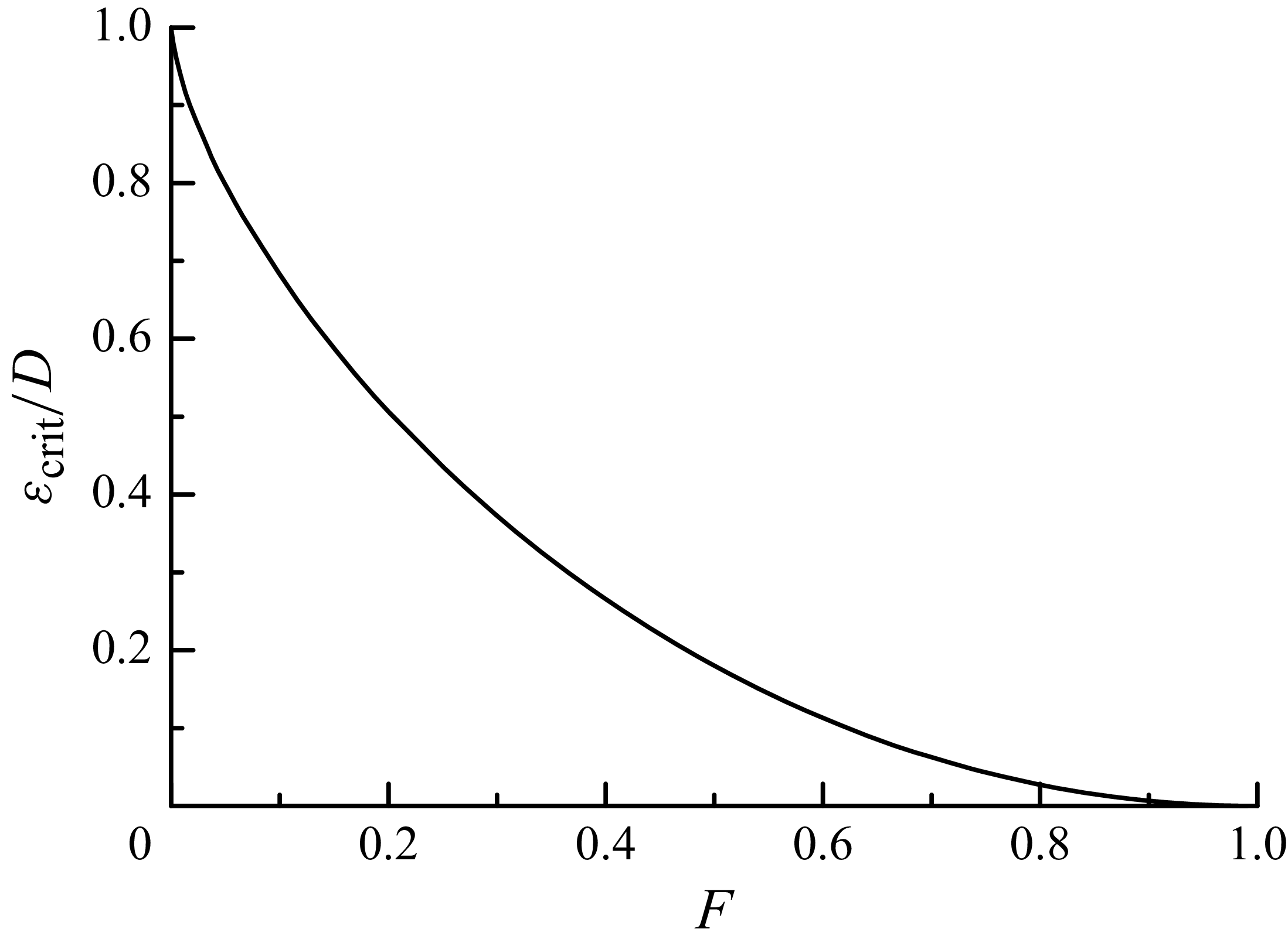
Figure 2 shows a plot of
 $\varepsilon _{\textit{crit}}/D$
as a function of the Froude number
 $F$
. It is seen that
 $\varepsilon _{\textit{crit}}$
is less than the fluid depth
 $D$
, in keeping with the flow configuration in figure 1. In addition,
 $\varepsilon _{\textit{crit}} \rightarrow 0$
when
 $F \rightarrow 1$
, consistent with the fact that the linear steady-state response breaks down at the critical
 $F=1$
.
Plot of the critical topography height
 $\varepsilon _{\textit{crit}}/D$
as a function of the Froude number
 $F$
according to (2.10).

We remark that the flow associated with the hydraulic steady state for
 $F\lt 1$
is subcritical at all streamwise locations
 $-\infty \lt x\lt \infty$
. Specifically, the local Froude number
 \begin{align} \widetilde {F}(x)= \widetilde {U}(x)/\sqrt {\widetilde {D}(x)} \lt 1. \end{align}
This certainly holds far upstream where
 $\varepsilon h\rightarrow 0$
so
 $\widetilde {F}=F\lt 1$
. Additionally,
 $\widetilde {F}$
is an increasing function of
 $\varepsilon h$
(since
 $\widetilde {U}$
increases while
 $\widetilde {D}$
decreases as
 $\varepsilon h$
is increased) and, at the maximum topography height
 $\varepsilon =\varepsilon _{\textit{crit}}$
,
 $\widetilde {F}=1$
from (2.6) and (2.10).
2.3. Formulation in the wavenumber domain
Carrying the expansions (2.5) in powers of
 $\mu$
to higher order cannot capture the wave response, as the wave amplitude is exponentially small with respect to
 $\mu$
. However, based on prior experience (KA2024, KA2025 and references therein), it is possible to diagnose the presence of radiating waves downstream by developing perturbation expansions in the wavenumber domain. For this purpose, rather than (2.1)–(2.3), we find it more convenient to use the non-local formulation of the water-wave problem (Ablowitz, Fokas & Musslimani Reference Ablowitz, Fokas and Musslimani2006). In the present setting, this formulation leads to three nonlinear equations in integral form for
 $\eta (x)$
,
 $u(x)=\varphi _x +\varphi _z \eta _x$
evaluated on the free surface
 $z=\eta$
, and
 $w(x)= \varphi _x+\varphi _z \varepsilon h_x$
evaluated on the topography
 $z=-D +\varepsilon h$
. Specifically,
 \begin{align} \displaystyle \int _{-\infty }^{\infty }{ \textrm {d}x \mbox{e}^{- \textrm{i}kx} \left \{(1+u)\sinh \left [\mu k(D+\eta )\right ] -(1+w)\sinh \left [\mu k \varepsilon h(x)\right ]\right \}}&=0, \end{align}
 \begin{align} \displaystyle \int _{-\infty }^{\infty }{ \textrm {d}x \mbox{e}^{- \textrm{i}kx} \left \{(1+u)\cosh \left [\mu k(D+\eta )\right ] -(1+w)\cosh \left [\mu k \varepsilon h(x)\right ]\right \}}&=0, \end{align}
 \begin{align} \displaystyle \hat {\eta }(k) +\hat {u}(k) +\int _{-\infty }^{\infty }{\textrm {d}x \mbox{e}^{- \textrm{i}kx} \left \{ \frac {u^2}{2} -\frac {\left [(1+u)\mu \eta _x \right ]^2}{2(1+\mu ^2 \eta _x^2)}\right \}} &=0, \end{align}
where
 $k$
is a (real) Fourier-like parameter and the Fourier transform in
 $x$
is defined as
 \begin{align} \displaystyle \hat {u}(k)= \frac {1}{2\pi } \int _{-\infty }^{\infty }{ u(x) \mbox{e}^{-\textrm{i}kx} \textrm {d}x}, \end{align}
with analogous expressions for
 $\hat {\eta }$
,
 $\hat {w}$
and
 $\hat {h}$
.
For topography of infinitesimal height
 $\varepsilon \rightarrow 0$
, linearizing the equation system (2.12) with respect to
 $ (\hat {\eta }, \hat {u}, \hat {w} )=O(\varepsilon )$
, yields
 $ ((\tanh \mu kD)/\mu k-1 )\hat {u}= \varepsilon \hat {h}\,\textrm { sech} \mu kD$
. Thus,
 $\hat {u}(k)$
has simple-pole singularities at
 $k=\pm \kappa _0 /\mu$
, where
 $\kappa _0$
solves
 \begin{align} \tanh \kappa _0 D=\kappa _0. \end{align}
For
 $F\lt 1$
(
 $D\gt 1$
), these poles are real. In addition, for smooth locally confined topography profile
 $h(x)$
, the magnitude of
 $\hat {h}(\pm \kappa _0/\mu )$
is exponentially small with respect to
 $\mu$
. Thus, upon inverting the Fourier integrals (in keeping with (2.4)), the pole residues contribute a radiating wave downstream
 \begin{align} u(x) \sim -\eta (x) \sim R \sin \left (\frac {\kappa _0}{\mu }x +\theta \right ) \quad \ (x\rightarrow \infty ), \end{align}
whose amplitude
 $R$
is exponentially small with respect to
 $\mu$
.
When the topography has finite height
 $\varepsilon \lt \varepsilon _{\textit{crit}}$
, the ensuing asymptotic analysis for
 $\mu \ll 1$
shows that the location of the poles specified by (2.14), and hence the wavelength of the radiating wave above, persists. However, the wave amplitude
 $R$
and the phase
 $\theta$
are controlled by a nonlinear beyond-all-orders mechanism. Importantly, for
 $\varepsilon$
close to
 $\varepsilon _{\textit{crit}}$
, the exponentially small (with respect to
 $\mu$
) factor of
 $R$
approaches
 $O(1)$
.
2.4. Topography profile
Kataoka & Akylas (Reference Kataoka and Akylas2024) analysed the wave response due to small-height topography (
 $0\lt \varepsilon \ll 1$
). They assumed that the topography profile
 $h(x)$
is a smooth locally confined function that is even in
 $x$
and whose (real) Fourier transform decays exponentially for large
 $k$
, like
 \begin{align} \hat {h}(k) \sim \left (A_0 |k|^{\alpha }+{\cdots} \right ) \exp (-\beta |k|) \ \quad (|k|\rightarrow \infty ), \end{align}
where
 $A_0$
,
 $\alpha$
and
 $\beta$
are real and
 $\beta \gt 0$
.
The wave response due to finite-height topography (
 $\varepsilon \lt \varepsilon _{\textit{crit}}$
) requires fundamentally different treatment from KA2024. For convenience in presenting the analysis, here
 $h(x)$
is taken to have the specific Fourier transform
 \begin{align} \hat {h}(k)=\frac {A_0}{2} \left (\frac {k}{\tanh (\pi k/2)} \right )^{\alpha } \textrm {sech} \frac {\pi k}{2}. \end{align}
This class of topography profiles (also used in KA2025) fits the asymptotic behaviour (2.16) with
 $\beta =\pi /2$
. Here,
 $\alpha$
is a free parameter while
 $A_0$
is fixed by the normalization
 $h(0)=1$
made earlier. (For
 $-30\lt \alpha \lt 30$
, it was checked numerically that
 $h(x)$
, defined by (2.17), attains its maximum value at
 $x=0$
, but we have no proof that this holds for all
 $\alpha$
.) For the particular values
 $\alpha =0$
and
 $1$
, the topography profiles corresponding to (2.17) are explicitly given by
 $h(x)=\textrm {sech}\,x$
and
 $\textrm {sech}^2 x$
, respectively. Generalization of the present analysis to other locally confined topography profiles is possible as long as they are smooth and even in
 $x$
(see comments in § 8).
3. Overview of exponential asymptotics
Before embarking on the detailed analysis, we outline the main steps of the exponential-asymptotics procedure for computing the radiating wave downstream under the flow conditions (1.3).
As noted earlier, perturbation expansions in powers of
 $\mu$
in the physical domain, like (2.5), give no sign of the wave response at any order of
 $\mu$
. This is in contrast to analogous expansions of
 $(\hat {u},\hat {w},\hat {\eta })$
, which become disordered (non-uniform) at large wavenumber (
 $k \gg 1$
) owing to the pole singularities at
 $k=\pm \kappa _0/\mu$
that give rise to the radiating wave (2.15). Here, it turns out that such non-uniformity first arises at
 $k=O(\mu ^{-4/5})$
(see § 4.1). Accordingly, similar to ‘two-timing’ in studies of nonlinear oscillations, we introduce the ‘stretched’ wavenumber
 \begin{align} K=\mu ^{4/5} k \end{align}
and propose the two-scale expansions
 \begin{align} (\hat {u},\hat {w},\hat {\eta })=\big (\hat {U}(K),\hat {W}(K),\hat {H}(K)\big ) \mu ^{6/5} \exp (-\gamma |k|) +{\cdots} , \end{align}
valid for
 $K=O(1)$
. Here,
 $(\hat {U},\hat {W},\hat {H})$
are
 $O(1)$
‘slowly varying’ amplitudes, while
 $\exp (-\gamma |k|)$
is a ‘fast’ exponential that derives from the asymptotic behaviour for
 $|k| \gg 1$
of the Fourier transform of the hydraulic solution.
Next, we derive (approximate) equations for
 $(\hat {U},\hat {W},\hat {H})$
by substituting (3.2) into the water-wave equations (2.12) in the wavenumber domain (see § 4.2). In simpler problems (e.g. Akylas & Yang Reference Akylas and Yang1995; Kataoka & Akylas Reference Kataoka and Akylas2022), such amplitude equations suffice to compute the (exponentially small) residues of the simple poles associated with the radiating wave. The wave amplitude and phase then are determined by the contribution of these residues upon inverting the Fourier transforms. Here, however, the poles in (2.14) occur at
 $k=\pm \kappa _0/\mu$
, whereas the expansions (3.2) hold only up to
 $K=O(1)$
; i.e.
 $k=O(\mu ^{-4/5}) \ll O(1/\mu )$
. Thus, a separate, ‘far-field’ analysis for
 $k=O(1/\mu )$
is necessary in order to capture the wave response.
To this end, the equations for
 $(\hat {U},\hat {W},\hat {H})$
are solved in the limit
 $K \gg 1$
(see § 4.3). These asymptotic solutions later serve as matching conditions with an appropriate far-field solution (see § 5). This solution is obtained most conveniently in the physical domain, by returning to expansions (2.5) and including a short-scale wave train downstream (the terms in the curly brackets below)
 \begin{align} \displaystyle \varphi (x,z)&=\varphi _0(x) +\mu ^2 \varphi _2(x,z) +{\cdots} +\mu \left \{\varPhi (x,z;\mu )\,\mbox{e}^{\textrm{i}\psi (x;\,\mu )/\mu } +\textrm {c.c.}\right \}, \\[-12pt] \nonumber \end{align}
 \begin{align} \displaystyle \eta (x)&=\eta _0 (x) +\mu ^2 \eta _2(x) +{\cdots} +\left \{Q(x;\mu )\,\mbox{e}^{ \textrm{i}\psi (x;\,\mu )/\mu } +\textrm { c.c.}\right \}. \end{align}
In these modified expansions, the short-scale wave train is modulated by the hydraulic disturbance (‘long wave’) present in the vicinity of the topography. Specifically, the phase function
 $\psi (x;\mu )$
describes the local wavenumber and
 $\varPhi$
,
 $Q$
are amplitude functions whose magnitude is expected to be exponentially small with respect to
 $\mu$
. Upon substituting (3.3) in the water-wave equations (2.1)–(2.3),
 $\psi$
,
 $\varPhi$
and
 $Q$
are readily computed by standard modulation theory. This confirms that far downstream (
 $x\rightarrow \infty$
) the short-scale disturbance is a uniform radiating wave train with wavenumber
 $\kappa _0/\mu$
, as claimed in (2.15). However,
 $\varPhi$
,
 $Q$
are proportional to a complex constant
 $C$
, which still remains undetermined. Importantly, the magnitude and phase of
 $C$
control the radiating wave amplitude
 $R$
and phase
 $\theta$
in (2.15).
This missing link is provided by matching the far-field solution above with the two-scale expansions (3.2) (see § 6). Specifically, we match the Fourier transform of the short-scale modulated wave train in (3.3) with the asymptotic solution for
 $K \gg 1$
of
 $(\hat {u},\hat {w},\hat {\eta })$
in (3.2), found earlier. This matching is achieved in a certain overlap wavenumber range where both these solutions are valid asymptotically. As a result, we obtain an explicit expression for the constant
 $C$
from which follow
 $R$
and
 $\theta$
(viz. (6.3)).
4. Two-scale analysis in the wavenumber domain
Carrying out the programme outlined in § 3, here we focus on the water-wave equations (2.12) in the wavenumber domain. The goal is to obtain a uniformly valid approximation to
 $(\hat {u},\hat {w},\hat {\eta })$
for
 $|k| \gg 1$
, which later (see § 6) will enable matching with the Fourier transform of the short-scale wave train downstream.
4.1. Scalings
We start by expanding
 $(\hat {u},\hat {w},\hat {\eta })$
in powers of
 $\mu ^2$
,
 \begin{align} \hat {u}(k;\mu )=\hat {u}_0 (k) +\mu ^2 \hat {u}_2 (k)+{\cdots} , \end{align}
with analogous expressions for
 $\hat {w}$
and
 $\hat {\eta }$
. While these straightforward expansions become disordered when
 $|k| \gg 1$
, by examining this disordering at the first few orders of
 $\mu ^2$
we deduce the appropriate scalings of
 $k$
and
 $(\hat {u},\hat {w},\hat {\eta })$
in the two-scale expansions (3.2). For this purpose, in (2.12) it is convenient to expand
 $\sinh$
,
 $\cosh$
and
 $(1+\mu ^2 \eta _x^2)^{-1}$
in powers of
 $\mu ^2 k^2$
,
 \begin{align} \mathbb{F}[(1+u)(D+\eta -\varepsilon h)-D] &=\mathbb{F}[(w-u)\varepsilon h] -\frac {\,\mu ^2 k^2}{6} \mathbb{F}\left [(1+u)\left ((D+\eta )^3-(\varepsilon h)^3\right )\right ] \nonumber \\ & \quad +O\big (\mu ^4 k^4 \hat {u} \big ), \end{align}
 \begin{align} \mathbb{F}[w-u]&= \frac {\mu ^2 k^2}{2} \mathbb{F}\left [(1+u)\left ((D+\eta )^2-(\varepsilon h)^2 \right )\right ] +O\big ( \mu ^4 k^4 \hat {u} \big ), \end{align}
 \begin{align} \mathbb{F}\left [\eta +u+\frac {u^2}{2}\right ]&= \frac {\mu ^2 k^2}{2} \mathbb{F}\left [(1+u)^2 \frac {\eta _x^2}{k^2} \right ] +O\big (\mu ^4 k^4 \hat {u} \big ), \\[12pt] \nonumber \end{align}
where
 $\mathbb{F}[\,\boldsymbol{\cdot }\,]$
denotes the Fourier transform as defined in (2.13).
Upon substituting (4.1) in (4.2), as expected, the leading-order solution
 $(\hat {u}_0, \hat {w}_0, \hat {\eta }_0)$
is the Fourier transform of the hydraulic solution (see § 2.2),
 \begin{align} u_0= \varphi _{0x},\qquad w_0=u_0, \qquad \eta _0=-u_0 -\frac {1}{2}u_0^2, \end{align}
where
 $u_0(x)$
is the perturbation horizontal velocity from the uniform stream, and the total horizontal velocity
 $\widetilde {U}(x)=1+u_0(x)$
satisfies the cubic (2.9). As discussed earlier, for
 $F\lt 1$
steady state is possible only if
 $\varepsilon \lt \varepsilon _{\textit{crit}}$
, where
 $\varepsilon _{\textit{crit}} (F)$
is given by (2.10) and is plotted in figure 2.
The behaviour of
 $(\hat {u}_0, \hat {w}_0, \hat {\eta }_0)$
as
 $|k| \rightarrow \infty$
is tied to the dominant singularities of
 $(u_0, w_0, \eta _0)$
. These singularities generally are of the branch-point type and are located on the imaginary axis closest to the origin of the complexified
 $x$
-plane, say at
 $x=\pm \textrm {i}\gamma$
. To determine
 $\gamma$
, there are two possible scenarios: (i)
 $\gamma$
is a root of
 $\varepsilon h(\textrm {i}\gamma )-\varepsilon _{\textit{crit}}=0$
such that
 $\gamma \lt \pi /2$
; (ii)
 $\gamma =\pi /2$
. The latter possibility arises because
 $x=\pm \textrm {i}\pi /2$
are the dominant singularities of
 $h(x)$
for the topography profiles chosen earlier (cf. (2.17)),
 \begin{align} h(x) &\sim \begin{cases} \displaystyle \frac {A_0 {\varGamma }(\alpha +1)}{(\pi /2 \pm \textrm {i}x)^{\alpha +1}}\qquad \ (\alpha \gt -1) \\ \displaystyle -A_0 \ln \left ( \pi /2 \pm \textrm {i}x \right )\quad \ \ (\alpha =-1) \end{cases} \left (x \rightarrow \pm \frac {\textrm {i}\pi }{2}\right )\!, \\[-12pt] \nonumber \end{align}
 \begin{align} \frac {\textrm {d}^m h}{ \textrm{d} (\mp \textrm {i}x)^m} &\sim \displaystyle \frac {A_0 {\varGamma }(\alpha +1+m)}{(\pi /2 \pm \textrm {i}x)^{\alpha +1+m}} \quad (\alpha \lt -1) \quad \left (x \rightarrow \pm \frac {\textrm {i}\pi }{2}\right )\!, \\[12pt] \nonumber \end{align}
where
 $m$
is the greatest integer less than or equal to
 $-\alpha$
and
 $\varGamma$
is the gamma function. Which of (i) and (ii) is appropriate depends on
 $\alpha$
and
 $\varepsilon$
, as discussed below.
When
 $\alpha \ge -1$
, according to (4.4a
),
 $h(x) \rightarrow \infty$
as
 $x \rightarrow \pm \textrm {i}\pi /2$
from the origin along the imaginary
 $x$
-axis. Since
 $h(0)=1$
, this implies that
 $h(x)$
reaches
 $\varepsilon _{\textit{crit}}/\varepsilon \gt 1$
at some
 $x=\pm \textrm { i}\gamma$
, say, where
 $\gamma (\alpha , \varepsilon )\lt \pi /2$
. Therefore, in this instance, scenario (i) above is valid for the entire range
 $0\lt \varepsilon \lt \varepsilon _{\textit{crit}}$
of topography heights.
According to (2.10), at
 $x=\pm \textrm {i}\gamma$
, where
 $\varepsilon h=\varepsilon _{\textit{crit}}$
, the cubic (2.9) has a double root,
 $\widetilde {U}_{\textit{crit}}=F^{-2/3}=D^{1/3}$
. Thus, close to
 $x=\pm \textrm {i}\gamma$
,
 \begin{align} \varepsilon h(x)&= \varepsilon _{\textit{crit}} \pm \frac {\varepsilon }{\textrm {i}} \left .\frac {{\textrm {d}}h}{{\textrm {d}}x}\right |_{x=\pm {\textrm {i}}\gamma } (\gamma \pm {\textrm {i}}x)+{\cdots} , \\[-12pt] \nonumber \end{align}
 \begin{align} \widetilde {U}(x)&=D^{1/3} -A \sqrt {\gamma \pm {\textrm {i}}x} +B (\gamma \pm {\textrm {i}}x)+{\cdots} . \\[10pt] \nonumber \end{align}
Upon substituting (4.5) in (2.9), collecting terms of equal order yields
 \begin{align} A^{\,2}= \pm \frac {2\textrm {i}}{3} \varepsilon \left .\frac {\textrm {d}h}{\textrm {d}x}\right |_{x=\pm \textrm {i}\gamma }, \qquad B=\frac {A^{\,2}}{3 D^{1/3}}. \end{align}
For certain values of
 $\alpha$
, including
 $\alpha =0$
which corresponds to the topography
 $h=\textrm {sech}\,x$
(used in the numerical computations in § 7), it is possible to find explicit expressions for
 $\gamma$
and
 $A$
. Generally, however, these constants are computed numerically by first determining
 $h(x)$
from
 $\hat {h}(k)$
in (2.17) and then solving
 $\varepsilon h(\textrm {i}\gamma ) -\varepsilon _{\textit{crit}}=0$
.
Making use of (4.5) and (4.6), the behaviour of the hydraulic solution (4.3) near
 $x=\pm \textrm {i}\gamma$
is
 \begin{align} u_0(x)&= w_0(x) \sim -1+D^{1/3} -A\sqrt {\gamma \pm \textrm {i}x} +\frac {A^{\,2}}{3D^{1/3}} (\gamma \pm \textrm {i}x) + {\cdots} \quad (x\rightarrow \pm \textrm {i}\gamma ), \\[-12pt] \nonumber \end{align}
 \begin{align} \eta _0 (x)&\sim \frac {1-D^{2/3}}{2} +D^{1/3}A\sqrt {\gamma \pm \textrm {i}x} -\frac {5}{6}A^{\,2}(\gamma \pm \textrm {i}x) +{\cdots} \quad (x\rightarrow \pm \textrm {i}\gamma ). \\[10pt] \nonumber \end{align}
Then, evaluating
 $ (\hat {u}_0(k), \hat {w}_0(k), \hat {\eta }_0(k) )$
, these branch-point singularities make the dominant contribution as
 $|k| \rightarrow \infty$
 \begin{align} \hat {u}_0(k)= \hat {w}_0(k)= -\frac {\hat {\eta }_0 (k)}{D^{1/3}} \sim \frac {A}{2\sqrt {\pi }} |k|^{-3/2} \exp (-\gamma |k|) \quad (|k|\rightarrow \infty ). \end{align}
At
 $O(\mu ^2)$
in expansion (4.1), the asymptotic behaviour of
 $\hat {u}_2 (k)$
as
 $|k|\rightarrow \infty$
is controlled by the dominant singularities of
 $u_2 (x)$
. From (4.2), along with (4.5)–(4.7), it follows that
 $(u_2, w_2, \eta _2)$
feature double poles at
 $x=\pm \textrm {i} \gamma$
(see Appendix A),
 \begin{align} u_2(x)=w_2(x)=-\frac {\eta _2(x)}{D^{1/3}} \sim \frac {D^{5/3}}{36(\gamma \pm \textrm {i}x)^2} \quad (x\rightarrow \pm \textrm {i}\gamma ), \end{align}
which yield
 \begin{align} \hat {u}_2(k)=\hat {w}_2(k)=-\frac {\hat {\eta }_2(k)}{D^{1/3}} \sim \frac {D^{5/3}}{36} |k|\exp (-\gamma |k|) \quad (|k|\rightarrow \infty ). \end{align}
Finally, combining (4.8) and (4.10) with (4.1), it is found that
 \begin{align} \hat {u}(k)=\hat {w}(k)=-\frac {\hat {\eta }(k)}{D^{1/3}} \sim \left \{ \frac {A}{2\sqrt {\pi }} |k|^{-3/2} +\frac {\mu ^2 D^{5/3}|k|}{36} +{\cdots} \right \} \exp (-\gamma |k|) \quad (|k|\rightarrow \infty ). \end{align}
Thus, expansion (4.1) becomes disordered when
 $k=O(\mu ^{-4/5})$
. This justifies the stretched wavenumber
 $K=\mu ^{4/5} k$
in (3.1). Furthermore, for
 $K=O(1)$
, (4.11) suggests replacing the ‘naïve’ expansion (4.1) with the two-scale expansion (3.2).
Coming now to the case
 $\alpha \lt -1$
,
 $h(x)$
remains finite at
 $x=\pm \textrm {i}\pi /2$
according to (4.4b
). Therefore, starting at the origin where
 $h(0)=1$
,
 $\varepsilon h(\pm \textrm {i}\gamma )=\varepsilon _{\textit{crit}}$
can be met for
 $\gamma \lt \pi /2$
(scenario (i) above) only when
 \begin{align} \varepsilon \gt \varepsilon _0 =\frac {\varepsilon _{\textit{crit}}}{h(\pm \textrm {i}\pi /2)}. \end{align}
(For the
 $\hat {h}(k)$
in (2.17), it is straightforward to verify that
 $h(\textrm {i}x)$
is monotonically increasing in
 $0\lt x\lt \pi /2$
.) Under condition (4.12), the dominant singularities of
 $(u_0, w_0, \eta _0)$
are branch points at
 $x=\pm \textrm {i}\gamma$
as in the case
 $\alpha \gt -1$
, so (4.7) remain valid and the asymptotic behaviours (4.11) still hold. Thus, when
 $\varepsilon _0 \lt \varepsilon \lt \varepsilon _{\textit{crit}}$
, the two-scale expansions (3.2) also apply to
 $\alpha \lt -1$
.
In contrast, for
 $\varepsilon \lt \varepsilon _0$
, the dominant singularities are no longer branch points at
 $x=\pm \textrm {i}\gamma$
 $(\gamma \lt \pi /2)$
. Instead, the behaviour of
 $(\hat {u}(k), \hat {w}(k), \hat {\eta }(k))$
for
 $|k|\rightarrow \infty$
is controlled by the singularities of the topography profile at
 $x=\pm \textrm {i}\pi /2$
(scenario (ii) above). The case
 $\varepsilon \lt \varepsilon _0$
will not be pursued here (see KA2025 for detailed discussion of an analogous situation in a model problem).
4.2. Amplitude equations
The two-scale expansions (3.2) approximate
 $(\hat {u}, \hat {w}, \hat {\eta })$
for
 $1 \ll |k|=O(\mu ^{-4/5})$
while the straightforward expansions (4.1) do so for
 $0 \le |k| \ll \mu ^{-4/5}$
. In addition, these expansions should match for
 $k$
in the overlap range
 \begin{align} 1 \ll |k|=O(1/\delta ) \ll \mu ^{-4/5}, \end{align}
where
 $\delta$
is a constant such that
 $\mu ^{4/5} \ll \delta \ll 1$
. In view of (4.11), matching requires the amplitude functions
 $(\hat {U}(K), \hat {W}(K), \hat {H}(K))$
in (3.2) to satisfy
 \begin{align} \hat {U}(K)=\hat {W}(K)=-\frac {\hat {H}(K)}{D^{1/3}} \sim \frac {A}{2\sqrt {\pi }}|K|^{-3/2} \quad (K\rightarrow 0). \end{align}
We now derive the equations that govern
 $(\hat {U},\hat {W},\hat {H})$
for
 $0\lt K=O(1)$
. This involves substituting expansions (3.2) and (4.1) in the water-wave equations (4.2) and approximating the convolution integrals that arise from the Fourier transform of nonlinear terms. In carrying out these approximations, however, the singular behaviour as
 $K \rightarrow 0$
in (4.14) causes convergence problems. To bypass this difficulty, we subtract out this behaviour
 \begin{align} \hat {u}(k;\mu )=\hat {u}_0 (k) +\hat {u}_s (k;\mu ) \end{align}
(with analogous expressions for
 $\hat {w}(k;\mu )$
and
 $\hat {\eta }(k;\mu )$
) and work with
 $(\hat {u}_s, \hat {w}_s, \hat {\eta }_s)$
. Then, from (4.11) it follows that the corresponding two-scale expansions are in the same form as (3.2),
 \begin{align} (\hat {u}_s, \hat {w}_s, \hat {\eta }_s)=(\hat {U}_s (K), \hat {W}_s(K), \hat {H}_s(K))\, \mu ^{6/5} \exp (-\gamma |k|)+{\cdots} , \end{align}
but the matching conditions for the amplitude functions are no longer singular,
 \begin{align} \hat {U}_s(K)=\hat {W}_s(K)=-\frac {\hat {H}_s(K)}{D^{1/3}} \sim \frac {D^{5/3}}{36} |K| \quad (K\rightarrow 0). \end{align}
Detailed derivation of the amplitude equations is given in Appendix B. The final result is that
 $\hat {U}_s(K)$
for
 $K\gt 0$
is governed by the Volterra-type integral equation
 \begin{align} &-\frac {K^2 D^2}{3} \hat {U}_s (K) +3D^{1/3} \int _0^{K}{ \left ( \frac {A}{\sqrt {\pi }} \lambda ^{-1/2}\frac {\textrm {d}\hat {U}_s (K-\lambda )}{\textrm { d}K} -\frac {\hat {U}_s(\lambda ) \hat {U}_s (K-\lambda )}{2} \right ) \textrm {d}\lambda }\nonumber\\&\quad =\frac {D^2 A}{6\sqrt {\pi }} K^{1/2}, \end{align}
subject to the matching condition (4.17). Once
 $\hat {U}_s (K)$
has been determined,
 \begin{align} \hat {W}_s (K)=\hat {U}_s (K), \qquad \hat {H}_s (K)=-D^{1/3} \hat {U}_s(K). \end{align}
It should be noted that the parameters
 $A$
and
 $D$
can be scaled out of (4.16) and (4.17) via
 \begin{align} (K, \lambda , \hat {U}_s) \rightarrow \frac {A^{\,2/5}}{\pi ^{1/5}} \left (D^{-2/3} K', D^{-2/3}\lambda ', D \hat {U}'_s \right )\!. \end{align}
This leads to the parameter-free equation (with primes dropped)
 \begin{align} -\frac {K^2}{3} \hat {U}_s (K) +3\int _0^{K}{ \left ( \lambda ^{-1/2}\frac {\textrm {d}\hat {U}_s (K-\lambda )}{\textrm {d}K} -\frac {\hat {U}_s(\lambda ) \hat {U}_s (K-\lambda )}{2} \right ) \textrm {d}\lambda } =\frac {K^{1/2}}{6}, \end{align}
and the matching condition
 \begin{align} \hat {U}_s (K) \sim \frac {K}{36} \quad (K \rightarrow 0). \end{align}
Thus, upon solving (4.21) subject to (4.22), the scaling (4.20) determines
 $\hat {U}_s (K)$
for all topography profiles
 $h(x)$
defined by (2.17).
4.3. Asymptotic solution for
 $K \gg 1$

In preparation for matching with the far-field solution, we now examine the asymptotic behaviour of
 $\hat {U}_s(K)$
for
 $K \gg 1$
. The integral equation (4.21) subject to condition (4.22) has precisely the form of an amplitude equation analysed in KA2025 (their equation (3.11) subject to their condition (3.6)). Following the same procedure as in KA2025, we find
 \begin{align} \hat {U}_s (K)\sim C_0 K \exp \left (\frac {K^5}{405 \pi } \right ) \quad (K\rightarrow \infty ), \end{align}
where
 \begin{align} C_0\approx 0.061. \end{align}
Then, reverting to the original variables in (4.20), this asymptotic solution reads
 \begin{align} \hat {U}_s (K)\sim C_0 D^{5/3} K \exp \left (\frac {D^{10/3}}{405 A^{\,2}}K^5 \right ) \quad (K\rightarrow \infty ) \end{align}
with
 $\hat {W}_s (K)$
and
 $\hat {H}_s (K)$
given by (4.19).
It should be noted that, when
 $k$
is near the expected pole of
 $\hat {u}(k)$
at
 $\kappa _0/\mu$
(cf. (2.14)), so
 $K=\mu ^{4/5} k=O(\mu ^{-1/5})\gg 1$
, the exponent above is
 $O(1/\mu )$
. However, the exponent of the fast exponential
 $\exp (-\gamma |k|)$
is
 $O(1/\mu )$
as well. This violates the separation of scales assumed in the two-scale expansions (4.16) and necessitates a rescaled, far-field analysis for
 $\kappa =\mu k=O(1)$
. The behaviour of
 $\hat {U}_s (K)$
for
 $K \gg 1$
in (4.25) then enables matching to the far-field solution for
 $\kappa \ll 1$
. These issues are discussed in §§ 5, 6.
5. Far-field analysis
Here, we construct a far-field solution that accounts for the radiating wave. This solution is obtained in the physical domain and then we compute its Fourier transform in preparation for matching with the asymptotic behaviour (4.25).
5.1. Downstream wave response in the physical domain
Returning to expansions (3.3), first we consider the long wave, represented by the terms outside the curly brackets. The leading-order solution is the hydraulic state (see § 2.2), and the inhomogeneous problem (2.7) for the
 $O(\mu ^2)$
correction is readily solved (as the solvability condition (2.8) is already satisfied)
 \begin{align} \varphi _2=\overline {\varphi }_2 (x)-\widetilde {U}_x \frac {z^2}{2} +\bigl(\widetilde {U}\eta _0\bigr)_{x\,} z, \end{align}
where
 $\overline {\varphi }_2 (x)$
is an undetermined function of
 $x$
.
Next, we focus on the short-scale wave train in expansions (3.3), anticipating that its amplitude is exponentially small with respect to
 $\mu$
. Upon substituting (3.3) in the water-wave equations (2.1)–(2.3), collecting terms proportional to
 $\exp (\textrm {i} \psi /\mu )$
yields, correct to
 $O(\mu |\varPhi |)$
,
 \begin{align} \varPhi _{zz} -\psi _x^2 \varPhi &=-\textrm {i}\mu (\psi _{\textit{xx}} \varPhi +2\psi _x \varPhi _x) \quad \ (-D+\varepsilon h\lt z\lt \eta _0), \end{align}
 \begin{align} \varPhi _z -\psi _x^2 \widetilde {U}^2 \varPhi &= \textrm {i}\mu \left \{ \psi _x \eta _{0x}\varPhi -\psi _x \widetilde {U}^2 \left (\left . \varPhi \right |_{z=\eta _0} \right )_x -\left (\frac { \left . \varPhi _z \right |_{z=\eta _0}}{\psi _x} \right )_x \right \} \quad (z=\eta _0), \end{align}
 \begin{align} \varPhi _z&=\textrm {i}\mu \psi _x \varepsilon h_x\varPhi \quad \ (z=-D+\varepsilon h). \end{align}
In addition,
 \begin{align} Q=-\textrm {i}\psi _x \widetilde {U}\varPhi -\mu (\widetilde {U}\varPhi _x +\varphi _{2z} \varPhi _z) \quad (z=\eta _0). \end{align}
The problem (5.2)–(5.4) is solved by expanding
 \begin{align} \varPhi (x,z;\mu )=\varPhi _0 (x,z)+\mu \varPhi _1 (x,z)+{\cdots} , \end{align}
with
 \begin{align} \psi (x;\mu )=\psi _0 (x)+\mu \psi _1 (x)+{\cdots} . \end{align}
Substituting (5.6)–(5.7) in (5.2)–(5.4), the leading-order solution is governed by
 \begin{align} \varPhi _{0zz} -\tilde {\kappa }^2 \varPhi _0 &=0 \quad (-D+\varepsilon h\lt z\lt \eta _0), \\[-28pt] \nonumber \end{align}
 \begin{align} \varPhi _{0z} -\tilde {\kappa }^2 \widetilde {U}^2 \varPhi _0&=0 \quad (z=\eta _0), \\[-28pt] \nonumber \end{align}
 \begin{align} \varPhi _{0z}&=0 \quad (z=-D+\varepsilon h). \\[0pt] \nonumber \end{align}
Hence,
 \begin{align} \varPhi _0=C \cosh \{\tilde {\kappa }(x) (z+D-\varepsilon h)\}, \end{align}
where
 $C$
is an undetermined (complex) constant. In addition,
 $\psi _0$
is given by
 \begin{align} \psi _0= \int _0^x{\tilde {\kappa }(x')\textrm {d}x'}, \end{align}
where
 $\tilde {\kappa }(x)/\mu$
is the local wavenumber of the short-scale wave train in keeping with the local dispersion relation
 \begin{align} \frac {\textrm {tanh}(\tilde {\kappa }\widetilde {D})}{\tilde {\kappa }} =\widetilde {U}^2, \end{align}
with
 $\widetilde {D}(x)=D+\eta _0 -\varepsilon h$
being the local fluid depth in the hydraulic state. As the local Froude number is subcritical (cf. (2.11)),
 $\tilde {\kappa }(x)$
is real.
Proceeding to
 $O(\mu )$
in expansions (5.6)–(5.7),
 $\varPhi _1$
satisfies the inhomogeneous boundary-value problem
 \begin{align} \varPhi _{1zz} -\tilde {\kappa }^2 \varPhi _1 &= I_1 C \quad (-D+\varepsilon h\lt z\lt \eta _0), \\[-28pt] \nonumber \end{align}
 \begin{align} \varPhi _{1z} -\tilde {\kappa }^2 \widetilde {U}^2\varPhi _1 &= I_2 C \quad (z=\eta _0), \\[-28pt] \nonumber \end{align}
 \begin{align} \varPhi _{1z} &= I_3 C \quad (z=-D+\varepsilon h), \\[0pt] \nonumber \end{align}
with
 \begin{align} I_1 &=\left ( 2\tilde {\kappa } \psi _{1x} -\textrm {i}\tilde {\kappa }_x \right )\cosh \{ \tilde {\kappa } (z+D-\varepsilon h) \} \nonumber \\ &\quad -2\textrm {i} \tilde {\kappa } \left \{\tilde {\kappa }_x (z+D-\varepsilon h) -\tilde {\kappa }\varepsilon h_x \right \} \sinh \{ \tilde {\kappa } (z+D-\varepsilon h) \}, \\[-12pt] \nonumber \end{align}
 \begin{align} I_2 &=2\psi _{1x} \sinh (\tilde {\kappa } \widetilde {D}) -\textrm {i}\tilde {\kappa } \widetilde {U} \left \{\widetilde {U} \cosh (\tilde {\kappa } \widetilde {D}) \right \}_x -\textrm {i} \left \{\sinh (\tilde {\kappa } \widetilde {D}) \right \}_x, \\[-12pt] \nonumber \end{align}
 \begin{align} I_3 &= \textrm {i} \tilde {\kappa }\varepsilon h_x. \\[9pt] \nonumber \end{align}
Since the corresponding homogeneous problem has a solution, namely (5.11), the forcing terms
 $I_1$
–
 $I_3$
above must observe a certain constraint in order for the problem (5.14)–(5.16) to have a solution as well. This solvability condition is deduced by multiplying (5.14) with
 $\varPhi _0$
in (5.11) and integrating across the fluid depth
 $-D+\varepsilon h\lt z\lt \eta _0$
. After two integrations by parts and making use of the boundary conditions (5.15) and (5.16), one obtains
 \begin{align} \!\!\!\!\!\!\!\!\!\!\!\! \int _{-D+\varepsilon h}^{\eta _0} {I_1 \cosh \left \{ \tilde {\kappa }(z+D-\varepsilon h) \right \} \textrm {d} z} -I_2 \cosh (\tilde {\kappa } \widetilde {D}) +I_3 =0. \end{align}
Inserting (5.17) in (5.18) and using (5.13), it follows that
 $\psi _1$
satisfies
 \begin{align} \varOmega (\tilde {\kappa } \widetilde {D})\,\psi _{1x} -\frac {\textrm {i}}{2} \left \{\varOmega (\tilde {\kappa } \widetilde {D})\right \}_x=0, \end{align}
where
 \begin{align} \varOmega (\tilde {\kappa } \widetilde {D})\equiv \sinh (\tilde {\kappa } \widetilde {D}) \cosh (\tilde {\kappa } \widetilde {D})-\tilde {\kappa } \widetilde {D} . \end{align}
Hence,
 \begin{align} \displaystyle \textrm {i} \psi _1 = -\frac {1}{2} \ln \frac {\varOmega (\tilde {\kappa } \widetilde {D})}{\varOmega (\kappa _0 D)}. \end{align}
As
 $\textrm {i}\psi _1 (x)$
is real,
 $\exp (\textrm {i}\psi _1)$
adds to the modulation of the short-wave amplitude in expansions (3.3). In fact, (5.19) written in the form
 \begin{align} \displaystyle \frac {\textrm{d}}{{\textrm {d}}x} \left \{ \varOmega (\tilde {\kappa }\widetilde {D}) \exp (2 {\textrm {i}} \psi _1) \right \} =0 \end{align}
can be shown to be equivalent to conservation of wave action in the steady modulated wave train downstream (Whitham Reference Whitham1974).
Combining (5.6), (5.7), (5.11), (5.12) and (5.21), the terms pertaining to the short-scale wave train in (3.3) take the form
 \begin{align} \varPhi \mbox{e}^{\textrm{i} \psi /\mu }&=C\cosh \{ \tilde {\kappa }(z+D-\varepsilon h) \} \sqrt { \frac {\varOmega (\kappa _0 D)}{\varOmega (\tilde {\kappa } \widetilde {D})} } \exp \left \{ \frac {\textrm {i}}{\mu } \int _0^x {\tilde {\kappa } (x')\textrm {d}x'} \right \} +{\cdots} , \\[-10pt] \nonumber \end{align}
 \begin{align} Q \mbox{e}^{ \textrm{i} \psi /\mu }&=-\textrm {i}C \tilde {\kappa } \widetilde {U} \cosh (\tilde {\kappa } \widetilde {D}) \sqrt { \frac {\varOmega (\kappa _0 D)}{\varOmega (\tilde {\kappa } \widetilde {D})} } \exp \left \{ \frac {\textrm {i}}{\mu } \int _0^x {\tilde {\kappa } (x')\textrm {d}x'} \right \} +{\cdots} . \end{align}
Far downstream
 $(x \rightarrow \infty )$
, the topography
 $\varepsilon h \rightarrow 0$
and the hydraulic state approaches the uniform stream (
 $\widetilde {U} \rightarrow 1$
). As a result, according to (5.13),
 $\tilde {\kappa }(x) \rightarrow \kappa _0$
where
 $\kappa _0$
 $(\gt 0)$
solves (2.14). Thus, making use of (5.23), the short-scale wave component in (3.3) approaches a uniform sinusoidal wave train
 \begin{align} u(x) &\sim \left .\varphi _x \right |_{z=\eta _0} \left (\sim -\eta (x)\right )\sim 2\kappa _0 |C|\cosh (\kappa _0 D)\nonumber \\ &\quad \times \sin \left \{ \frac {\kappa _0}{\mu } x +\frac {1}{\mu } \int _0^{\infty }{\left ( \tilde {\kappa }(x') -\kappa _0 \right )\textrm {d}x'} +\arg (-C) \right \} \ \ \ (x \rightarrow \infty ), \end{align}
where
 $C=|C|\exp (\textrm {i}\,\textrm {arg}C)$
. Furthermore, upon comparing (5.24) with (2.15), the radiating wave amplitude
 $R$
and phase shift
 $\theta$
are related to
 $C$
via
 \begin{align} R=2\kappa _0 |C| \cosh (\kappa _0 D), \qquad \theta = \frac {1}{\mu } \int _0^{\infty }{ \left (\tilde {\kappa }(x') -\kappa _0 \right ) \textrm {d}x'} +\arg (-C). \end{align}
5.2. Far-field solution in the wavenumber domain
We now compute the Fourier transform of the downstream modulated short-scale wave train found above. Specifically, using (5.23) in (3.3),
 \begin{align} \hat {u}&= \displaystyle \mathbb{F}\left [\left .(\varphi _x +\varphi _z \eta _x) \right |_{z=\eta } \right ] \nonumber \\ & \sim \displaystyle \frac {C}{2\pi } \int _{-\infty }^{\infty }{ \textrm {i}\tilde {\kappa } \cosh (\tilde {\kappa }\widetilde {D}) \sqrt { \frac {\varOmega (\kappa _0 D)}{\varOmega (\tilde {\kappa } \widetilde {D})} } \exp \left \{ \textrm {i} \left (-kx+ \frac {1}{\mu }\int _0^x{\tilde {\kappa }(x') \textrm {d}x'} \right ) \right \} \textrm {d}x}. \end{align}
It should be noted that, of the two terms which are complex conjugate of each other in the curly brackets in (3.3), only the one
 $\propto \exp (\textrm {i}\psi /\mu )$
is included above, as the corresponding local wavenumber
 $\tilde {\kappa }/\mu \gt 0$
. Thus, only this term is appropriate for matching with (4.25), which was derived for
 $K\gt 0$
.
In view of (4.7) and (5.13), the integrand in (5.26) features branch points at the zeroes of
 $\tilde {\kappa }(x)$
, i.e.
 $x=\pm \textrm {i}\gamma$
. Accordingly, we introduce a branch cut between these two points on the imaginary
 $x$
-axis, and deform the integration path to pass below
 $x=-\textrm {i}\gamma$
(see figure 2 of KA2025). Furthermore, due to the radiation condition (2.4), the radiating wave train stretches only downstream (
 $\textrm {Re}\, x\gt 0$
) so the lower integration limit is replaced by
 $-\textrm {i}\gamma$
.
Next, we examine the asymptotic behaviour of the resulting contour integral
 \begin{align} \hat {u}\sim \frac {C}{2\pi } \int _{-\textrm{i}\gamma }^{\infty }{ \textrm {i}\tilde {\kappa } \cosh (\tilde {\kappa }\widetilde {D}) \sqrt { \frac {\varOmega (\kappa _0 D)}{\varOmega (\tilde {\kappa } \widetilde {D})} } \exp \left \{ \frac {\textrm {i}}{\mu } \left (-\kappa x+\int _0^x{\tilde {\kappa }(x') \textrm {d}x'} \right ) \right \} \textrm {d}x}, \end{align}
when
 $\kappa = \mu k$
satisfies
 \begin{align} \mu ^{1/5} \ll \kappa \ll 1. \end{align}
In terms of
 $K=\mu ^{4/5} k$
, this wavenumber range translates to
 $1\ll K \ll \mu ^{-1/5}$
, so it is a common range of validity of the far-field solution (5.27) and the asymptotic solution (4.25) obtained earlier using the two-scale expansions (4.16). Therefore, these two solutions should match in the wavenumber range (5.28).
For
 $\kappa$
satisfying (5.28), the integral in (5.27) is approximated following the procedure used for an analogous integral in KA2025 (see their (4.10)). Specifically, we first expand the integrand around the branch point
 $x=-\textrm {i} \gamma$
and then evaluate the resulting integral asymptotically for
 $\kappa ^5/\mu \gg 1$
using Laplace’s method (see Appendix C). The final result is
 \begin{align} \hat {u}\sim -\frac {C}{3} \sqrt {\frac {\mu }{3\pi } \varOmega (\kappa _0 D)} \,\frac {D^{2/3}}{A} \,\kappa \! \kern3pt &\exp \left (-\frac {\textrm {i}}{\mu } \int _{- \textrm{i}\gamma }^0 {\tilde {\kappa }(x') \textrm {d}x'} \right ) \exp \left ( \frac {D^{10/3}}{405 \mu A^2} \kappa ^5 \right ) \mbox{e}^{-\gamma k} \nonumber \\ & \left (\mu ^{1/5} \ll \kappa \ll 1 \right )\!. \end{align}
6. Radiating wave
We now compute the radiating wave amplitude and phase. Returning to the two-scale expansions (4.16) and making use of the asymptotic solution (4.25) for
 $\hat {U}_s (K)$
, yields
 \begin{align} \hat {u}_s \sim \mu ^{6/5} C_0 D^{5/3} K \exp \left (\frac {D^{10/3}}{405 A^{\,2}} K^5 \right ) \mbox{e}^{-\gamma k} \quad \left (1 \ll K \ll \mu ^{-1/5} \right )\!. \end{align}
In fact, this asymptotic result also applies to
 $\hat {u}=\hat {u}_0 +\hat {u}_s$
(cf. (4.15)) because, in view of (4.8),
 $\hat {u}_0$
is subdominant relative to
 $\hat {u}_s$
above. Thus, expression (6.1), written in terms of
 $\kappa =\mu ^{1/5} K$
, should match with expression (5.29) because the two-scale expansion (4.16) and the far-field solution (5.27) are both valid in the wavenumber range (5.28), as argued earlier. This matching requirement determines the constant
 $C$
:
 \begin{align} C=-3\sqrt {\frac {3 \pi \mu }{ \varOmega (\kappa _0 D) }} \,C_0 A D \exp \left ( \frac {\textrm {i}}{\mu }\int _{- \textrm{i}\gamma }^0 {\tilde {\kappa }(x') \textrm {d}x'} \right )\!. \end{align}
Then, the radiating wave amplitude and phase follow from (5.25),
 \begin{align} R&=6\sqrt {\frac {3 \pi \mu }{ \varOmega (\kappa _0 D) }}\,C_0 A D \kappa _0 \cosh (\kappa _0 D) \exp \left (-\frac {q(\alpha ,\varepsilon )}{\mu } \right )\!, \end{align}
 \begin{align} \theta &= \frac {1}{\mu } \int _0^\infty {\left ( \tilde {\kappa }(s)-\kappa _0 \right ) \textrm {d}s}, \end{align}
where
 $C_0$
is given by (4.24) and
 \begin{align} q(\alpha ,\varepsilon )= \int _0^\gamma {\tilde {\kappa }(\textrm {i} s) \textrm {d}s}. \end{align}
It should be noted that
 $q(\alpha , \varepsilon )$
is real because
 $\tilde {\kappa }(x)$
is an even function according to (5.13). Furthermore,
 $q(\alpha ,\varepsilon )\gt 0$
since
 $\tilde {\kappa }(x)\gt 0$
when
 $x=\textrm {i} s$
 $(0\lt s\lt \gamma )$
.
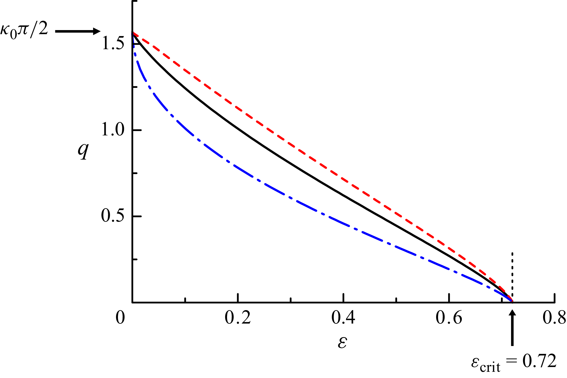
Figure 3 plots
 $q$
as a function of
 $0\lt \varepsilon \lt \varepsilon _{\textit{crit}}$
when
 $F=0.5$
 $(D=4)$
and for
 $\alpha =1$
,
 $0$
and
 $-0.5$
. It is seen that
 $q$
decreases monotonically, so the exponential factor of
 $R$
in (6.3a
) grows with increasing
 $\varepsilon$
. Thus, finite-height topography can enhance exponentially the radiating downstream wave. In addition, according to (6.3b
), the phase shift
 $\theta$
is controlled by the deviation of the local wavenumber from its constant value far downstream,
 $(\tilde {\kappa }-\kappa _0)/\mu$
. For
 $\varepsilon \rightarrow 0$
,
 $\tilde {\kappa } \rightarrow \kappa _0$
according to (5.13), so (6.3b
) recovers the linear result
 $\theta =0$
(cf. (6.6)).
The exponent
 $q$
(defined in (6.4)) that controls the exponential factor of the wave amplitude
 $R$
, as a function of the peak topography height
 $\varepsilon$
, when
 $F=0.5$
 $(D=4)$
:
 $\alpha =1$
(blue dash-dotted line); 0 (black solid line);
 $-0.5$
(red dashed line). The vertical dotted line indicates the critical topography height
 $\varepsilon _{\textit{crit}}=0.72$
.

Importantly, when
 $\varepsilon$
approaches
 $\varepsilon _{\textit{crit}}$
, the roots
 $x=\pm \textrm {i}\gamma$
of
 $\varepsilon h(x)-\varepsilon _{\textit{crit}}=0$
approach the origin
 $(\gamma \rightarrow 0)$
. Thus, according to (6.4) and as shown in figure 3,
 \begin{align} q(\alpha ,\varepsilon )\rightarrow 0 \quad \left (\varepsilon \rightarrow \varepsilon _{\textit{crit}} \right )\!, \end{align}
so the exponential factor of
 $R$
approaches
 $O(1)$
. Even though the present theory formally breaks down in this limit, one still expects
 $R$
to increase rapidly as
 $\varepsilon \rightarrow \varepsilon _{\textit{crit}}$
, resulting in a steep wave train downstream. It should be noted that this perhaps unexpected effect (confirmed by numerical computations in § 7) arises, however small
 $\mu$
(which controls dispersion) may be.
In the other extreme, when the topography height
 $\varepsilon \rightarrow 0$
, the roots
 $x=\pm \textrm {i}\gamma$
of
 $\varepsilon h(x)-\varepsilon _{\textit{crit}} =0$
approach
 $x=\pm \textrm {i}\pi /2$
 $(\gamma \rightarrow \pi /2)$
, where
 $h(x) \rightarrow \infty$
according to (4.4a
). Furthermore, from (5.13),
 $\tilde {\kappa } \rightarrow \kappa _0$
, so
 $q \rightarrow \kappa _0 \pi /2$
(figure 3). Thus, the leading-order exponential factor
 $R=O (\exp (-\kappa _0 \pi /2\mu ) )$
in (6.3a
) is set by the behaviour of
 $\hat {h}(k)$
for
 $|k| \rightarrow \infty$
in (2.16), regardless of the peak topography height
 $\varepsilon$
. This agrees with the classical linear solution for
 $\varepsilon \rightarrow 0$
,
 \begin{align} R_{\textit{lin}}= \frac {4\pi \varepsilon A_0}{\mu ^{\alpha +1}} C_{\textit{lin}} \exp \left ( \frac {-\kappa _0 \pi }{2\mu } \right )\!,\qquad \theta _{{ lin}}=0, \end{align}
where
 \begin{align} C_{\textit{lin}}=\frac {2\kappa _0^{\alpha +1}\sinh \kappa _0 D}{\displaystyle \sinh 2\kappa _0 D-2\kappa _0 D}, \end{align}
as well as with the wave response for topography of small height
 $0\lt \varepsilon \ll 1$
(KA2024). In the latter case, however, the wave amplitude (save for the leading-order exponential factor) is controlled by a nonlinear mechanism.
It should be noted that, while the exponential factor in (6.3a
) reduces for
 $0\lt \varepsilon \ll 1$
to that found in KA2024, the asymptotic solutions for small- and finite-height topography do not merge smoothly. To handle this difficulty, an ‘intermediate’ solution that takes into account the effects of the nearly coalescing singularities at
 $x=\pm \textrm {i}\gamma$
and
 $x=\pm \textrm {i}\pi /2$
, would be needed. Treating problems with coalescing singularities via exponential asymptotics was discussed in Trinh & Chapman (Reference Trinh and Chapman2015).
7. Numerical results
We now turn to direct numerical computations based on the full water-wave equations in order to assess the validity of the asymptotic theory. Additionally, motivated by the asymptotic results, we investigate numerically the appearance of steep waves downstream when
 $\varepsilon \approx \varepsilon _{\textit{crit}}$
.
Our computations used the boundary-integral method of Belward & Forbes (Reference Belward and Forbes1993) for steady two-layer flow over topography (setting the upper-layer density to zero in their formulation). We employed uniform computational meshes, typically for
 $-25D\lt x/\mu \lt 40D$
and allocating 25 discrete points to each wavelength of the downstream wave.
In the interest of brevity, here we report on numerical computations only for the topography profile
 $h(x)=\textrm {sech}\,x$
(corresponding to
 $\alpha =0$
,
 $A_0 =1$
in (2.17)). In this instance, there are explicit expressions for the parameters
 $\gamma$
and
 $A$
in (4.5)–(4.6):
 \begin{align} \displaystyle \gamma = \cos ^{-1} \left (\frac {\varepsilon }{\varepsilon _{\textit{crit}}} \right )\!,\qquad A= \sqrt {\frac {2\varepsilon _{{ crit}}}{3}} \,\left \{ \left (\frac {\varepsilon _{\textit{crit}}}{\varepsilon } \right )^2 -1 \right \}^{1/4}. \end{align}
Furthermore, the Froude number is fixed to
 $F=0.5$
 $(D=4)$
, which specifies
 $\varepsilon _{\textit{crit}} =0.72$
according to (2.10). Our results for other values of
 $\alpha \gt -1$
and
 $F\lt 1$
are qualitatively similar to those discussed below.
Figure 4 plots theoretical and numerically computed downstream wave profiles for
 $\mu =0.1$
and topography peak heights
 $\varepsilon =0.30$
, 0.50 and 0.65. It is noted that the largest of these,
 $\varepsilon$
, is not far from
 $\varepsilon _{\textit{crit}}=0.72$
. The theoretical wave profiles in figure 4 are the predictions of the finite-height theory (6.3), the small-height theory (obtained from (5.13) in KA2024 by multiplying
 $R$
with
 $\varepsilon$
and setting
 $n=0$
) and the linear response (6.6) (with
 $\alpha =0$
,
 $A_0=1$
).
Downstream wave profiles
 $\eta (x)$
in free-surface flow over topography with
 $h(x)=\textrm {sech}x$
and peak height (a)
 $\varepsilon =0.30$
, (b) 0.50 and (c) 0.65, when
 $F=0.5$
(
 $D=4$
) and
 $\mu =0.1$
: exact numerical solution (black solid line); finite-height theory (6.3) (red dash-dotted line); small-height theory (blue dashed line); linear theory (6.6) (green dotted line).

Figure 4 shows that the small-height theory is most accurate for the smallest of the three topography heights,
 $\varepsilon =0.30$
, while the finite-height theory works best for the largest,
 $\varepsilon =0.65$
. For the intermediate
 $\varepsilon =0.50$
, which falls in the transition range from the small- to the finite-height solution, both these solutions provide reasonably good, but not excellent, approximations to the radiating wave. By contrast, the linear solution grossly underestimates the wave response for all three values of
 $\varepsilon$
. Specifically, for
 $\varepsilon =0.30$
, the small-height theoretical predictions for the wave amplitude
 $R$
and the phase shift
 $\theta$
agree very well with the numerical solution while the finite-height solution clearly overestimates
 $R$
(by roughly a factor of 2). On the other hand, for
 $\varepsilon =0.65$
, the finite-height theoretical predictions for
 $R$
and
 $\theta$
are in excellent agreement with the numerical solution, unlike the small-height solution which underestimates
 $R$
(by roughly a factor of 0.5) and also exhibits a noticeable phase lag relative to the numerical wave profile.
In figure 5, we compare theoretical with numerical results for the ratio of the nonlinear to the linear wave amplitude
 $R/R_{\textit{lin}}$
as a function of the topography peak height
 $0\lt \varepsilon \lt \varepsilon _{\textit{crit}}=0.72$
, for three values of
 $\mu =0.1$
, 0.15 and 0.2. As expected, the agreement of asymptotic with numerical results improves as
 $\mu$
is decreased. Furthermore, the small-height theory (KA2024) provides a reliable approximation for
 $0\lt \varepsilon \lesssim 0.5$
(see the insets in figure 5) while the finite-height result (6.3a
) does so for
 $0.5 \lt \varepsilon \lt \varepsilon _{\textit{crit}}$
. However, as noted earlier, the small- and finite-height asymptotic results do not merge smoothly.
Ratio of nonlinear to linear wave amplitude as a function of the topography peak height. Here (a)
 $\mu =0.1$
, (b) 0.15 and (c) 0.2: exact numerical solution (circle); finite-height theory (6.3) (solid line); small-height theory (dashed line). The insets zoom in on
 $\varepsilon \ll 1$
. The vertical dotted lines denote the critical height
 $\varepsilon _{\textit{crit}}=0.72$
(cf. (2.10)).

Figure 5 indicates that the radiating wave amplitude
 $R$
increases rapidly when
 $\varepsilon$
approaches
 $\varepsilon _{\textit{crit}}$
. In this limit, in view of (6.5), the exponentially small factor of
 $R$
in (6.3a
) becomes
 $O(1)$
and our exponential-asymptotics procedure breaks down. Additionally, the steady hydraulic solution (4.3), which forms the starting point of the present analysis, is not valid when
 $\varepsilon \gt \varepsilon _{\textit{crit}}$
. Accordingly, below we explore by numerical means the behaviour of the downstream wave for
 $\varepsilon \approx \varepsilon _{\textit{crit}}$
.
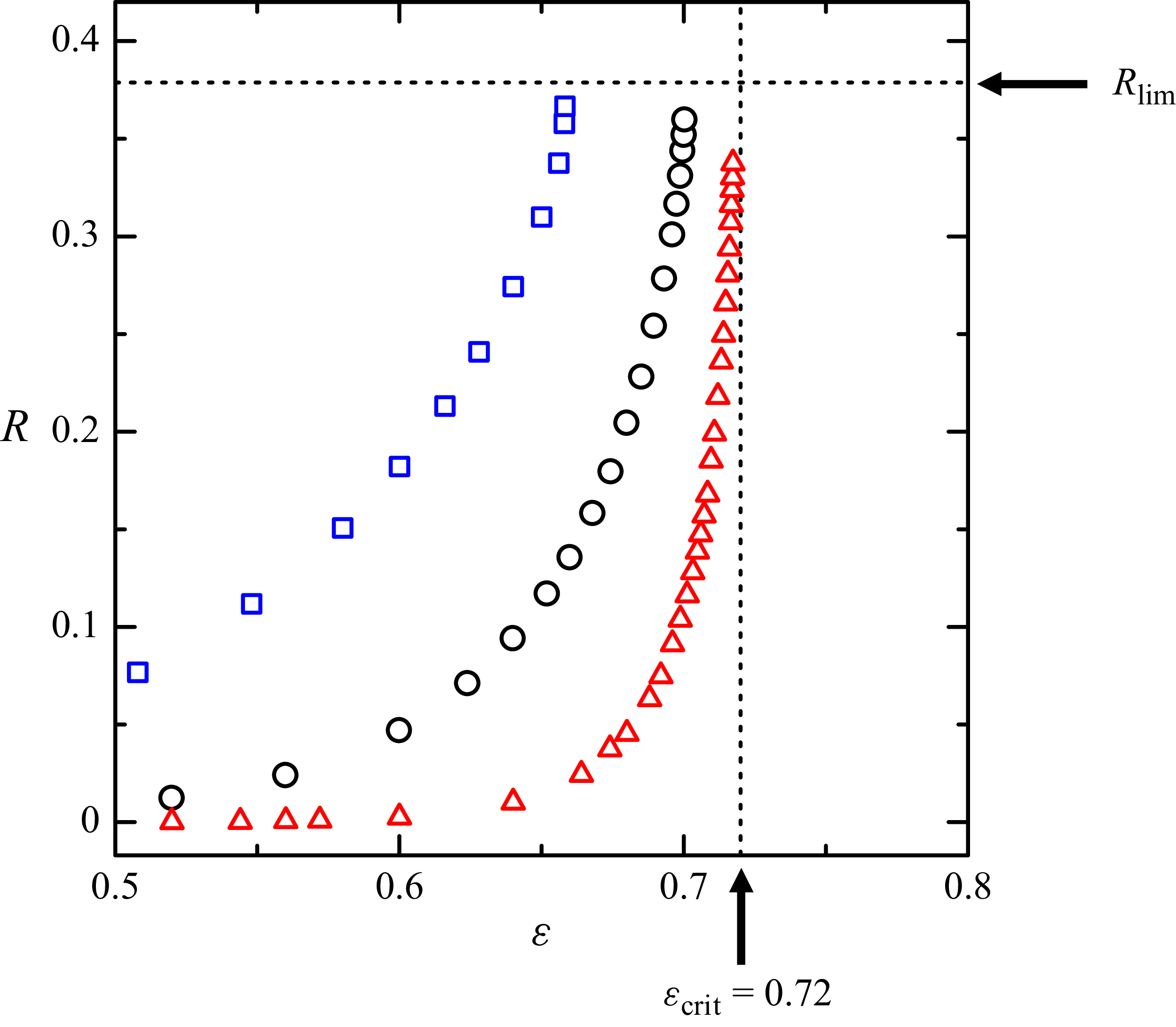
Figure 6 plots numerical results for the downstream wave amplitude
 $R$
, defined as half the crest-to-trough height, as a function of the topography peak height
 $\varepsilon$
in the vicinity of
 $\varepsilon _{\textit{crit}}$
, for three values of
 $\mu =0.05$
, 0.1 and 0.2. These results indicate that for each
 $\mu$
there is a limiting topography height,
 $\varepsilon _{\textit{lim}}$
, beyond which no steady wave train can be computed. Furthermore, as
 $\mu$
is decreased,
 $\varepsilon _{\textit{lim}}$
approaches
 $\varepsilon _{\textit{crit}}$
. (While
 $\varepsilon _{ { lim}} \lt \varepsilon _{\textit{crit}}$
in figure 6, computations for other
 $F$
and
 $\mu$
, not shown here, indicate that
 $\varepsilon _{\textit{lim}}$
can exceed
 $\varepsilon _{\textit{crit}}$
.)
Numerically computed wave amplitude
 $R$
(defined as half the crest-to-trough height) versus topography peak height
 $\varepsilon$
in the vicinity of
 $\varepsilon _{\textit{crit}}=0.72$
:
 $\mu =0.05$
(red triangle); 0.1 (black circle); 0.2 (blue rectangle). The horizontal dotted line is an estimate of the limiting amplitude
 $R_{\textit{lim}}$
of the Stokes wave.

According to figure 6, as
 $\varepsilon$
approaches
 $\varepsilon _{\textit{lim}}$
,
 $R$
increases dramatically and reaches
 $O(1)$
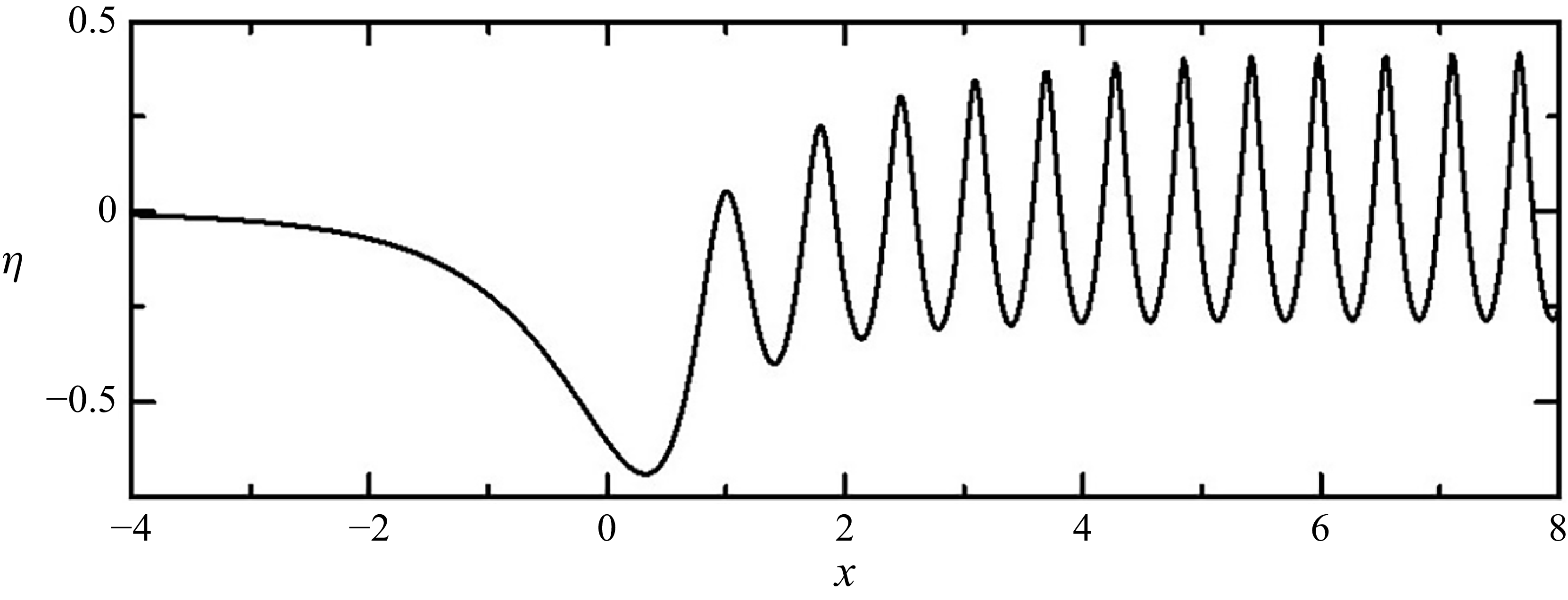
, suggesting that the wave train downstream becomes fully nonlinear. This is confirmed in figure 7, which displays the computed free-surface profile for
 $\mu =0.1$
and
 $\varepsilon$
slightly below 0.70, the value of
 $\varepsilon _{\textit{lim}}$
for this
 $\mu$
. Indeed, the wave downstream has steep crests and broad troughs, resembling a steep Stokes wave. Naturally, these nonlinear features are not captured by our exponential-asymptotics theory. Nevertheless, the present theory does hint at the rapid increase of the wave amplitude as
 $\varepsilon$
approaches
 $\varepsilon _{\textit{lim}} \approx \varepsilon _{\textit{crit}}$
for
 $\mu \ll 1$
. Figure 6 also indicates the limiting amplitude
 $R_{\textit{lim}}$
of steady Stokes periodic waves for
 $D=4$
(which essentially corresponds to deep water), as estimated from the numerical computations of Williams (Reference Williams1981). As expected,
 $R_{\textit{lim}}$
provides an upper bound for
 $R$
, and the computed wave downstream for
 $\varepsilon$
slightly below
 $\varepsilon _{\textit{lim}}$
(figure 7) is close to the limiting Stokes wave.
Numerically computed free-surface profile
 $\eta (x)$
when
 $\mu =0.1$
and the topography peak height
 $\varepsilon$
is slightly below
 $\varepsilon _{\textit{lim}}=0.70$
for this
 $\mu$
(figure 6).

Finally, we discuss briefly the wave response when the peak topography height
 $\varepsilon$
exceeds
 $\varepsilon _{\textit{lim}}$
, so no steady solution can be computed. Instead, an initial-value problem was solved starting from rest and turning on the uniform stream impulsively, based on the time-dependent water-wave equations. This unsteady flow was computed using the numerical method of Dold & Peregrine (Reference Dold and Peregrine1986), which can handle breaking waves. This method introduces fluid particles on the free surface and their motion is determined by integrating the Lagrangian time derivatives of their positions. We used approximately 35 particles per wavelength of the downstream wave, with 2000 particles in total. This resolution enabled us to capture with sufficient accuracy the overhanging motion of a crest. The time step (using
 $U_{\ast }/g$
as the time scale) was initially set to
 $\bigtriangleup t=0.1$
and then reduced to
 $\bigtriangleup t=0.01$
once an overhanging crest appeared. As a check, the numerical procedure was applied to the initial-value problem for values of
 $\varepsilon \lt \varepsilon _{{ lim}}$
and it was verified that the flow approached the steady state computed earlier.
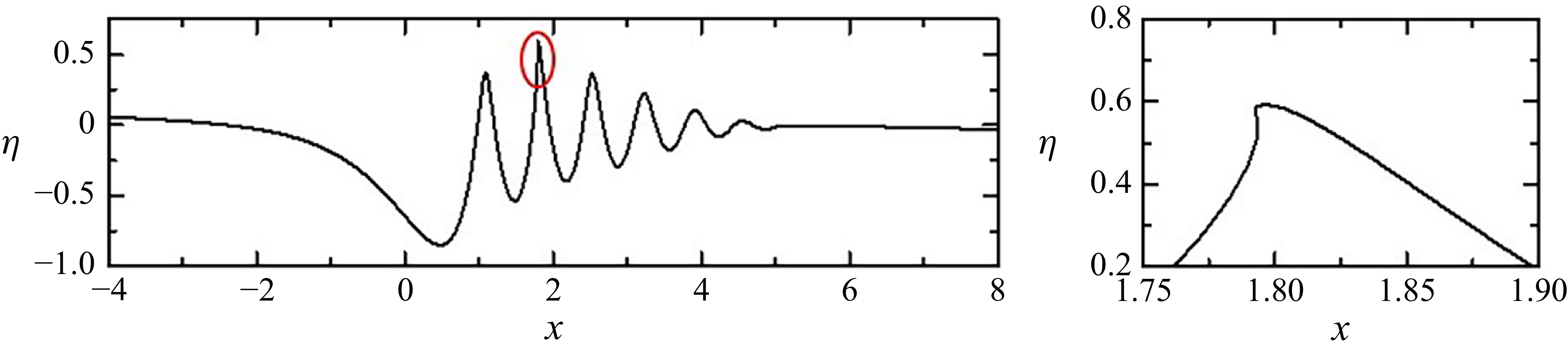
Figure 8 shows the computed unsteady free-surface profile for
 $\mu =0.1$
and
 $\varepsilon =0.76\gt \varepsilon _{\textit{lim}}=0.70$
, at
 $t=107$
. At this time, an ‘undular bore’ with steep crests has formed downstream of the topography and one of these crests is starting to overhang, signalling the onset of wave breaking. Interestingly, this wave-breaking phenomenon is not associated with the long wave disturbance over the topography predicted by the hydraulic solution for
 $\mu \ll 1$
. Instead, the wave breaking is triggered by the (formally exponentially small with respect to
 $\mu$
) short-scale wave train downstream, which regardless of
 $\mu$
grows sharply and reaches
 $O(1)$
amplitude as the topography peak height gets close to
 $\varepsilon _{\textit{lim}}$
.
Unsteady free-surface profile
 $\eta (x,t)$
at
 $t=107$
, when a downstream wave crest (marked with red circle) first overhangs. Panel (b) zooms in on the overhanging crest. The flow was computed by initiating the uniform stream impulsively at
 $t=0$
, for
 $F=0.5$
,
 $\mu =0.1$
and topography peak height
 $\varepsilon =0.76 \gt \varepsilon _{\textit{lim}} =0.70$
.

8. Concluding remarks
This study revisits steady two-dimensional free-surface flow due to a uniform stream flowing over smooth, locally confined bottom topography. Earlier theoretical treatments were based on the nonlinear shallow-water equations, which are derived from the full potential flow equations in the limit of long waves. Thus, on physical grounds, one expects this so-called hydraulic theory to be a valid approximation for flow over topography of large horizontal extent (
 $\mu \ll 1$
) and Froude number
 $F=O(1)$
. Under these conditions and subcritical flow (
 $F\lt 1$
), the hydraulic solution is a steady disturbance confined in the vicinity of the topography if the topography peak height
 $\varepsilon$
is below a certain critical value,
 $\varepsilon _{\textit{crit}} (F)$
; when
 $\varepsilon \gt \varepsilon _{\textit{crit}}$
, the oncoming flow is partially blocked by the topography and hydraulic jumps form upstream and downstream.
The nonlinear shallow-water equations neglect the effects of dispersion altogether. The present analysis focuses on how these effects (controlled by
 $\mu \ll 1$
) may influence the locally confined steady wave disturbance predicted by the hydraulic theory for
 $F \lt 1$
and
 $\varepsilon \lt \varepsilon _{\textit{crit}}$
. Specifically, based on the dispersion relation of gravity water waves, for
 $F \lt 1$
, it is possible for a steady radiating wave to appear downstream. However, when
 $\mu \ll 1$
, this wave is much shorter than the topography width, which suggests that (for smooth topography profile whose Fourier transform decays exponentially at large wavenumber) the wave amplitude is exponentially small with respect to
 $\mu$
. Thus, one might expect that this dispersive wave downstream is insignificant relative to the
 $O(1)$
hydraulic disturbance over the topography.
Contrary to the heuristic argument above, our asymptotic analysis of the full potential flow equations for
 $\mu \ll 1$
reveals that the short-scale dispersive wave downstream is in fact a prominent part of the wave response, particularly as
 $\varepsilon$
approaches
 $\varepsilon _{\textit{crit}}$
. While the wave amplitude is indeed exponentially small with respect to
 $\mu$
,
 $R = O (\exp (-q/\mu ) )$
, the exponent
 $q$
is controlled by nonlinearity via the topography peak height parameter
 $\varepsilon$
. Specifically,
 $q$
is a decreasing function of
 $\varepsilon$
and
 $q \rightarrow 0$
as
 $\varepsilon \rightarrow \varepsilon _{\textit{crit}}$
. Thus, increasing the topography peak height amplifies exponentially the radiating wave amplitude, and as
 $\varepsilon$
approaches
 $\varepsilon _{\textit{crit}}$
this (formally exponentially small) wave reaches the same level as the hydraulic wave disturbance. As a result, the nonlinear shallow-water equations break down in the vicinity of
 $\varepsilon _{\textit{crit}}$
regardless of
 $\mu \ll 1$
.
The present analysis makes use of exponential asymptotics combined with inner–outer matching. The ‘inner’ solution is obtained by a multiple-scale expansion in the wavenumber domain, while the ‘outer’ (far-field) solution accounts for the modulation of the short-scale radiating wave train by the hydraulic disturbance in the physical domain. Upon computing the Fourier transform of the outer solution, the amplitude and phase of the radiating wave are determined by matching these two solutions in an appropriate overlap wavenumber range.
Here, the exponential-asymptotics treatment focuses on a specific class of topography profiles (cf. (2.17)). However, the same procedure applies to any smooth even topography profile
 $h(x)$
(e.g. a Gaussian) at finite
 $\varepsilon \lt \varepsilon _{\textit{crit}}$
such that the dominant singularities are branch points at
 $x = \pm \textrm {i}\gamma$
(scenario (i) in § 4). Under this condition (generally satisfied for
 $\varepsilon =O(1)$
below
 $\varepsilon _{\textit{crit}}$
), the inner solution (4.25), including the constant
 $C_0$
in (4.24), is universal. Furthermore, the far-field solution (5.29) is valid for any smooth even
 $h(x)$
. Thus, the analytical expressions (6.3) for the radiating wave amplitude and phase remain intact (with
 $\gamma$
,
 $A$
and
 $\tilde {\kappa }(x)$
depending on the specific
 $h(x)$
).
The results of the asymptotic analysis are supported by numerical solutions of the full steady potential flow equations. In particular, these computations confirm that when
 $\varepsilon$
approaches
 $\varepsilon _{\textit{crit}}$
the radiating wave grows sharply and becomes comparable with the hydraulic disturbance. Furthermore, there is a limiting
 $\varepsilon$
,
 $\varepsilon _{\textit{lim}} \approx \varepsilon _{\textrm { crit}}$
, depending on
 $\mu$
and
 $F$
, such that no steady solution that decays to zero far upstream and remains finite downstream can be computed when
 $\varepsilon \gt \varepsilon _{\textit{lim}}$
. For
 $\varepsilon$
just below
 $\varepsilon _{\textit{lim}}$
, the computed steady wave downstream resembles a steep Stokes periodic wave. In addition, unsteady numerical computations turning on the uniform stream far upstream impulsively, indicate that when
 $\varepsilon$
is slightly above
 $\varepsilon _{\textit{lim}}$
an oscillatory disturbance forms downstream, which steepens and breaks.
Finally, the present theoretical findings bring out the need for experiments that focus on the wave response downstream. While existing experimental observations (Long Reference Long1954, Reference Long1970) do not report any downstream waves, our results suggest that such waves play an important part within a range of topography peak heights around
 $\varepsilon _{\textit{crit}}$
. Specifically, as
 $\varepsilon$
is increased towards and past
 $\varepsilon _{\textit{crit}}$
, we expect generation of steep waves followed by wave breaking downstream, before upstream influence due to blocking of the flow by the topography eventually sets in.
Declaration of interests
The authors report no conflict of interest.
Data availability statement
The data that support the findings of this study are available on request from T.K.
Appendix A. Derivation of (4.9)
We derive (4.9) from (4.2) expressed in the physical domain. To leading order
 $O(1)$
, (4.2a
) recovers the hydraulic solution
 $\widetilde {U}=1+u_0$
(cf. (2.9)). Correct to
 $O(\mu ^2)$
, the left-hand side of (4.2a
), with the aid of (4.2c
), then takes the form
 \begin{align} (1+u)(D+\eta -\varepsilon h) -D \rightarrow \mu ^2 \left \{ G(x)u_2 +\frac {\widetilde {U}^3}{2}\eta _{0x}^2 \right \}, \end{align}
where
 \begin{align} G(x)= \widetilde {D}-\widetilde {U}^2 \end{align}
and
 $\widetilde {D}=D+\eta _0 -\varepsilon h$
is the local depth in the hydraulic solution. Furthermore, the right-hand side of (4.2a
), with the aid of (4.2b
), is expressed as
 \begin{eqnarray} &&\!\! \displaystyle (w-u)\varepsilon h +\frac {\mu ^2}{6} \left \{ (1+u)\left ( (D+\eta )^3-(\varepsilon h)^3 \right )\right \}_{\textit{xx}} \nonumber \\ &&\qquad \qquad \rightarrow \displaystyle \mu ^2 D\left (-\frac {1}{2} (D+\eta _0 +\varepsilon h)_{\textit{xx}} \varepsilon h +\frac {1}{6} \left \{ \widetilde {D}^2 +3(D+\eta _0)\varepsilon h \right \}_{\textit{xx}} \right )\!. \end{eqnarray}
Therefore, combining (A1) and (A3),
 $u_2$
satisfies
 \begin{align} G(x)u_2 =\frac {D}{6} \frac { \textrm{d}^2 \widetilde {D}^2}{\textrm {d}x^2} +r_0 (x), \end{align}
where
 \begin{align} r_0 (x)= -\frac {D}{2}(D+\eta _0 +\varepsilon h)_{xx\,} \varepsilon h +\frac {D}{2}\left \{ (D+\eta _0)\varepsilon h \right \}_{\textit{xx}} -\frac {\widetilde {U}^3}{2}\eta _{0x}^2. \end{align}
Finally, evaluating (A4) close to the singularities
 $x \rightarrow \pm \textrm {i}\gamma$
using (4.5) and (4.7),
 \begin{align} G(x)\sim 3D^{1/3} A\sqrt {\gamma \pm \textrm {i}x}, \quad \!\!\! \frac { \textrm{d}^2 \widetilde {D}^2}{\textrm {d}x^2} \sim \frac {DA}{2(\gamma \pm \textrm {i}x)^{3/2}}, \quad \!\!\! r_0 (x) \sim O \big ( \!(\gamma \pm \textrm {i}x)^{-1} \big ) \quad\!\!\! (x\rightarrow \pm \textrm {i}\gamma ), \end{align}
by dominant balance we obtain (4.9) for
 $u_2$
. Furthermore, using (4.2b
,
c
), we deduce (4.9) for
 $w_2$
and
 $\eta _2$
.
Appendix B. Derivation of amplitude equation (4.18)
We derive the amplitude equation (4.18) by substituting (4.15) along with (4.16) in (4.2). To this end, with the aid of (4.2c ) and (2.9), the left-hand side of (4.2a ) becomes
 \begin{align} \mathbb{F}\left [M(x) -D \right ]= \mathbb{F} \left [ G(x)u_s -\frac {3\widetilde {U}}{2} u_s^2 -\frac {u_s^3}{2} +\mu ^2 \frac {(1+u)^3}{2}\eta _{x}^2 \right ]\!, \end{align}
where
 \begin{align} M(x)= (1+u)(D+\eta -\varepsilon h), \end{align}
and
 $G(x)$
is defined by (A2). Next, using a similar procedure to that leading to (A3), the right-hand side of (4.2a
) becomes
 \begin{align} & \displaystyle \mathbb{F}[(w-u)\varepsilon h] -\frac {\,\mu ^2 k^2}{6} \mathbb{F}\left [(1+u)\left ((D+\eta )^3-(\varepsilon h)^3\right )\right ] \nonumber \\ &\! =\displaystyle \mu ^2 \mathbb{F}\left [-\frac {1}{2}\{M(x)(D+\eta +\varepsilon h)\}_{xx\,} \varepsilon h +\frac {1}{6} \left \{M(x) \left ( (D+\eta -\varepsilon h)^2 +3(D+\eta )\varepsilon h \right ) \right \}_{\textit{xx}} \right ]\!, \end{align}
where we used (4.2b ) and (2.9). Combining (B1) and (B3), yields
 \begin{align} \mathbb{F} \left [ G(x)u_s -\frac {3\widetilde {U}}{2} u_s^2 -\frac {u_s^3}{2} \right ]= \mu ^2 \mathbb{F} \left [ \frac {1}{6} \left \{M(x)(D+\eta -\varepsilon h)^2 \right \}_{\textit{xx}} +r(x) \right ]+O\big (\mu ^4 k^4 \hat {u} \big ), \end{align}
where
 \begin{align} r(x)= -\frac {1}{2}\{M(x)(D+\eta +\varepsilon h)\}_{xx\,} \varepsilon h +\frac {1}{2}\left \{M(x) (D+\eta )\varepsilon h \right \}_{\textit{xx}}-\frac {(1+u)^3}{2}\eta _{x}^2. \end{align}
Now, based on (B4), we derive the amplitude equation (4.18) for
 $\hat {U}_s (K)$
with
 $K=O(1)\gt 0$
. According to the straightforward expansion (4.1) and the two-scale expansion (4.16),
 \begin{eqnarray} &&\hat {u}_s (k;\mu )\sim \begin{cases} O(\mu ^2) \quad (|k| \lesssim 1/\delta )\\[3pt] \mu ^{6/5} \hat {U}_s (K) \mbox{e}^{-\gamma |k|} \quad (|k| \gtrsim 1/\delta ), \end{cases} \end{eqnarray}
where
 $\mu ^{4/5} \ll \delta \ll 1$
(cf. (4.13)). Also, according to (A6),
 $\hat {G}(k)$
behaves like
 \begin{eqnarray} &&\hat {G}(k) \sim \begin{cases} O(1) \quad (|k| \lesssim 1/\delta ) \\[5pt] \displaystyle \left ( -\frac {3D^{1/3} A}{2\sqrt {\pi } |k|^{3/2}} +{\cdots} \right ) \mbox{e}^{-\gamma |k|} \quad (|k| \gtrsim 1/\delta ). \end{cases} \end{eqnarray}
Then,
 $\mathbb{F}[G(x)u_s]$
on the left-hand side of (B4) for
 $K=O(1)\gt 0$
 $(k=O(\mu ^{-4/5}))$
is evaluated as
 \begin{align} \mathbb{F}[G(x)u_s] &\equiv \int _{-\infty }^{\infty }{\hat {G}(l) \hat {u}_s (k-l) \textrm {d}l} \nonumber \\ &\sim \mu ^{8/5} \mbox{e}^{-\gamma k} \left \{ \mu ^{-2/5} \int _{-\infty }^{1/\delta }{\hat {G}(l) \mbox{e}^{\gamma l} \hat {U}_s (K-\mu ^{4/5} l) \textrm {d}l} \right . \nonumber \\ &\quad \left . +\int _{\mu ^{4/5}/\delta }^{K-\mu ^{4/5}/\delta } {\left ( -\frac {3D^{1/3} A}{2\sqrt {\pi } \lambda ^{3/2}} +{\cdots} \right ) \hat {U}_s(K-\lambda )\textrm {d} \lambda } +O\bigl(\mu ^{8/5}\bigr) \right \}\!. \end{align}
Integrating by parts the integral on the far right-hand side of (B8) and using
 $\int _{-\infty }^{\infty }{\hat {G}(l) \mbox{e}^{\gamma l}\textrm {d}l}=G(-\textrm {i}\gamma )=0$
(see (A6)), we have
 \begin{align} \mathbb{F}[G(x)u_s] \sim \mu ^{8/5} \mbox{e}^{-\gamma k} \frac {3D^{1/3} A}{\sqrt {\pi }} \int _0^K {\lambda ^{-1/2} \frac {\textrm {d} \hat {U}_s (K-\lambda )}{\textrm {d} K} \textrm {d}\lambda }. \end{align}
Next, by a similar procedure, the second term
 $\mathbb{F}[-(3\widetilde {U}/2) u_s^2]$
on the left-hand side of (B4) for
 $K=O(1)\gt 0$
is evaluated as
 \begin{align} \mathbb{F}\left [-\frac {3}{2} \widetilde {U} u_s^2 \right ] \sim -\frac {3}{2} \mu ^{8/5} \mbox{e}^{-\gamma k} D^{1/3} \int _0^K {\hat {U}_s (\lambda ) \hat {U}_s (K-\lambda ) \textrm {d}\lambda }, \end{align}
where (B6) and
 $\widetilde {U} \sim D^{1/3}$
 $(x \rightarrow \pm \textrm {i}\gamma )$
(see (4.5b
)) are used. The last term
 $\mathbb{F}[-u_s^3 /2]$
on the left-hand side of (B4) is subdominant relative to (B9) and (B10).
Regarding the right-hand side of (B4), near the singularity
 $x\rightarrow -\textrm {i}\gamma$
,
 \begin{align} \frac {1}{6} \left \{M(x)(D+\eta -\varepsilon h)^2 \right \}_{\textit{xx}} \sim \frac {D^2 A}{12(\gamma -\textrm {i}x)^{3/2}} +\frac {D^{5/3}}{3} \frac { \textrm{ d}^2 \eta _s}{\textrm {d}x^2} \quad (x\rightarrow -\textrm {i}\gamma ),&& \end{align}
 \begin{align} r(x) \sim O\left ( (\gamma -\textrm {i}x)^{-1} \right ) + O\left ( (\sqrt {\gamma -\textrm {i}x}\, \eta _s )_{\textit{xx}} \right ) \quad (x\rightarrow -\textrm { i}\gamma ), \qquad && \end{align}
where (4.5), (4.7) and
 $M(x) \sim D+O(\sqrt {\gamma -\textrm {i}x}\,\eta _s)$
 $(x \rightarrow -\textrm {i}\gamma )$
are used. Thus,
 $r(x)$
in (B11b
) is subdominant in comparison with (B11a
). Accordingly, making also use of (4.19), the right-hand side of (B4) for
 $K=O(1)\gt 0$
 $(k=O(\mu ^{-4/5}))$
is evaluated as
 \begin{align} \mu ^2 \mathbb{F}\left [ \frac {1}{6} \left \{ M(x)(D+\eta -\varepsilon h)^2 \right \}_{\textit{xx}} +r(x) \right ] \sim \mu ^{8/5} \mbox{e}^{-\gamma k} \left ( \frac {D^2 A}{6\sqrt {\pi }} K^{1/2} +\frac {D^2}{3} K^2 \hat {U}_s (K) \right )\!. \end{align}
Substituting (B9), (B10) and (B12) into (B4), yields (4.18).
Appendix C. Derivation of (5.29)
We derive (5.29) by evaluating the integral (5.27) asymptotically under condition (5.28). To this end, we focus on the behaviour of the integrand in the neighbourhood of the branch point at
 $x=-\textrm {i}\gamma$
. Specifically, with
 $x=-\textrm {i}\gamma +\textrm {i}s$
, the exponent in (5.27) reads
 \begin{align} -\gamma k -\frac {\textrm {i}}{\mu } \int _{-\textrm {i}\gamma }^0 {\tilde {\kappa }(x') \textrm {d}x'} +\Delta , \end{align}
where
 \begin{align} \varDelta =\frac {\kappa }{\mu } s -\frac {1}{\mu } \int _0^s {\tilde {\kappa } (-\textrm {i}\gamma +\textrm {i}s')\textrm {d}s'}. \end{align}
For
 $s \ll 1$
, in view of (5.13) with (4.7),
 $\tilde {\kappa }(-\textrm {i}\gamma +\textrm {i}s') \sim 3D^{-5/6}\sqrt {A}\, s'^{1/4}$
, so that
 \begin{align} \varDelta \sim \frac {\kappa }{\mu } s -\frac {12}{5\mu D^{5/6}} \sqrt {A}\, s^{5/4}. \end{align}
Then, setting
 $s=(D^{10/3} \kappa ^4 /3^4 A^{\,2})\,y$
, it follows that
 \begin{align} \sqrt { \frac {\varOmega (\kappa _0 D)}{\varOmega (\tilde {\kappa } \widetilde {D})} }\, \mbox{e}^{\Delta } \sim J \left ( \frac {D^{10/3} \kappa ^4}{3^4 A^{\,2}} \,y \right )^{-3/8} \exp \left \{ \frac {D^{10/3}}{3^4 A^{\,2}} \frac {\kappa ^5}{\mu } \left (y-\frac {4}{5} y^{5/4} \right ) \right \}, \end{align}
where we used
 $\varOmega (\tilde {\kappa }\widetilde {D}) \sim 18A^{3/2} s^{3/4}/D^{1/2}$
 $(s \ll 1)$
from (4.7) and (5.20), and
 \begin{align} J= \frac { \sqrt { \varOmega (\kappa _0 D) }\, D^{1/4} } {3\sqrt {2} \,A^{3/4}} \end{align}
is a real constant. The exponent in (C4) has a maximum at
 $y=1$
and
 $\kappa ^5/\mu \gg 1$
according to (5.28). Thus, we may use Laplace’s method to approximate the integral in (5.27) with the exponential factor (C4), which leads to (5.29).