


1. Introduction
A system is said to be robust with respect to perturbations of a set of parameters, if small changes to those parameters do not result in significant changes in the behavior of the system. Robustness is a core requirement of safety-critical systems, including neural networks deployed in high-stakes applications (Dietterich, Reference Dietterich2017; Heaven, Reference Heaven2019). As a result, several methods have been suggested for measuring robustness, e.g., through adversarial attacks (Carlini and Wagner, Reference Carlini and Wagner2017; Goodfellow et al., Reference Goodfellow, Shlens and Szegedy2015) or via attack-agnostic methods (Hein and Andriushchenko, Reference Hein and Andriushchenko2017; Jordan and Dimakis, Reference Jordan and Dimakis2020, Reference Jordan, Dimakis, Meila and Zhang2021; Ko et al., Reference Ko, Lyu, Weng, Daniel, Wong, Lin, Chaudhuri and Salakhutdinov2019; Weng et al., Reference Weng, Zhang, Chen, Song, Hsieh, Boning, Dhillon and Daniel2018b). A common and effective attack-agnostic approach involves estimation of the local Lipschitz constant of the network. This makes sense as larger Lipschitz constants signify more sensitivity to input values. As such, a useful estimate of the Lipschitz constant should be a tight upper bound. A lower bound of the Lipschitz constant results in false negatives – which are more serious than false positives – and a very loose upper bound generates too many false positives, which renders the estimate ineffective. Sound and accurate computation of the Lipschitz constant is also essential in Lipschitz regularization of neural networks (Araujo et al., Reference Araujo, Négrevergne, Chevaleyre and Atif2021; Pauli et al., Reference Pauli, Koch, Berberich, Kohler and Allgöwer2022).
Of particular interest is the estimation of Lipschitz constant of non-differentiable networks, such as
 ${\mathrm{ReLU}}$
networks. Computing the Lipschitz constant of
 ${\mathrm{ReLU}}$
networks is not just an NP-hard problem (Virmaux and Scaman, Reference Virmaux, Scaman, Bengio, Wallach, Larochelle, Grauman, Bianchi and Garnett2018), it is strongly inapproximable (Jordan and Dimakis, Reference Jordan and Dimakis2020, Theorem 4). As a result, methods of Lipschitz analysis fall into two disjoint categories:
-
(1) Scalable, but not validated, e.g., Weng et al. (Reference Weng, Zhang, Chen, Song, Hsieh, Boning, Dhillon and Daniel2018b), Chen et al. (Reference Chen, Lasserre, Magron, Pauwels, Larochelle, Ranzato, Hadsell, Balcan and Lin2020), Latorre et al. (Reference Latorre, Rolland and Cevher2020);
-
(2) Validated, but not scalable, e.g., Hein and Andriushchenko (Reference Hein and Andriushchenko2017), Jordan and Dimakis (Reference Jordan and Dimakis2020, Reference Jordan, Dimakis, Meila and Zhang2021), and the method of the current article.
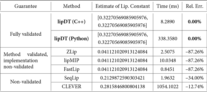
The validated methods – though not scalable – are essential in providing the ground truth for verification of the scalable methods. For instance, consider the scalable Cross Lipschitz Extreme Value for nEtwork Robustness Clever method of Weng et al. (Reference Weng, Zhang, Chen, Song, Hsieh, Boning, Dhillon and Daniel2018b). Jordan and Dimakis (Reference Jordan and Dimakis2020) demonstrate that, on certain parts of the input domain, Clever outputs inaccurate results, even on small networks. The method of Jordan and Dimakis (Reference Jordan and Dimakis2020, Reference Jordan, Dimakis, Meila and Zhang2021), in turn, although based on a validated theory, is implemented using floating-point arithmetic, which is prone to inaccuracies, as will be demonstrated in Section 5. It is well-known that floating-point errors lead to vulnerability in safety-critical neural networks (Jia and Rinard, Reference Jia, Rinard, Dragoi, Mukherjee and Namjoshi2021; Zombori et al., Reference Zombori, Bánhelyi, Csendes, Megyeri and Jelasity2021).
Based on the theory of continuous domains, we develop a framework for robustness analysis of neural networks, within which we design an algorithm for estimation of local Lipschitz constant of feedforward regressors. We prove the soundness of the algorithm. Moreover, we prove completeness of the algorithm over differentiable networks and also over general position
 ${\mathrm{ReLU}}$
networks.
To avoid the pitfalls of floating-point errors, we implement our algorithm using arbitrary-precision interval arithmetic (with outward rounding) which guarantees soundness of the implementation as well. As such, our method is fully validated, that is, not only does it follow a validated theory but also it has a validated implementation.
1.1 Related work
A common approach to robustness analysis of neural networks is based on estimation of Lipschitz constants. A mathematical justification of this reduction is provided in Hein and Andriushchenko (Reference Hein and Andriushchenko2017, Theorem 2.1) and Weng et al. (Reference Weng, Zhang, Chen, Song, Hsieh, Boning, Dhillon and Daniel2018b, Theorem 3.2). The global Lipschitz constant of a network may be estimated by multiplying the Lipschitz constants of individual layers. This approach, taken by Szegedy et al. (Reference Szegedy, Zaremba, Sutskever, Bruna, Erhan, Goodfellow and Fergus2014), is scalable but provides loose bounds. In Clever (Weng et al., Reference Weng, Zhang, Chen, Song, Hsieh, Boning, Dhillon and Daniel2018b), a statistical approach is adopted using Extreme Value Theory (de Haan and Ferreira, 2006). While Clever is scalable, it may underestimate the Lipschitz constant significantly (Jordan and Dimakis, Reference Jordan and Dimakis2020). A sound approach to Lipschitz estimation was introduced by Hein and Andriushchenko (Reference Hein and Andriushchenko2017), but the method applies only to differentiable shallow networks. Semidefinite programming has been used by Fazlyab et al. (Reference Fazlyab, Robey, Hassani, Morari, Pappas, Wallach, Larochelle, Beygelzimer, d’Alché-Buc, Fox and Garnett2019) and Hashemi et al. (Reference Hashemi, Ruths, Fazlyab, Jadbabaie, Lygeros, Pappas, Parrilo, Recht, Tomlin and Zeilinger2021) to obtain tight upper bounds on the Lipschitz constant of a network.
Of particular relevance to our work are methods that are based on abstract interpretation (Cousot and Cousot, Reference Cousot and Cousot1977). The study of abstract interpretation in a domain-theoretic framework goes back (at least) to Burn et al. (Reference Burn, Hankin and Abramsky1986), Abramsky (Reference Abramsky1990). In the current context, the main idea behind abstract interpretation is to enclose values and then follow how these enclosures propagate through the layers of a given network. Various types of enclosures may be used, e.g., hyperboxes, zonotopes, or polytopes, in increasing order of accuracy, and decreasing order of efficiency (Gehr et al., Reference Gehr, Mirman, Drachsler-Cohen and Tsankov2018; Mirman et al., Reference Mirman, Gehr, Vechev, Dy and Krause2018; Singh et al., Reference Singh, Gehr, Püschel and Vechev2019). Theoretically, methods that are based on interval analysis (Lee et al., Reference Lee, Lee, Park, Larochelle, Ranzato, Hadsell, Balcan and Lin2020; Prabhakar and Afzal, Reference Prabhakar and Afzal2019; Wang et al., Reference Wang, Pei, Whitehouse, Yang and Jana2018) or convex outer polytopes (Sotoudeh and Thakur, Reference Sotoudeh, Thakur, Pichardie and Sighireanu2020; Wong and Kolter, Reference Wong, Kolter, Dy and Krause2018) are also subsumed by the framework of abstract interpretation. These methods, however, are applied over the network itself, rather than its gradient.
In contrast, in Chaudhuri et al. (Reference Chaudhuri, Gulwani and Lublinerman2012, Reference Chaudhuri, Gulwani, Lublinerman and Navidpour2011), abstract interpretations were used for estimating Lipschitz constants of programs with control flow, which include neural networks as special cases. Jordan and Dimakis (Reference Jordan and Dimakis2020, Reference Jordan, Dimakis, Meila and Zhang2021) have used Clarke’s generalized gradient (Clarke, Reference Clarke1990) to analyze non-differentiable (e.g.,
 ${\mathrm{ReLU}}$
) networks. Their overapproximation of the Clarke-gradient also follows the spirit of abstract interpretation. Based on dual numbers, sound automatic differentiation, and Clarke Jacobian, Laurel et al. (Reference Laurel, Yang, Singh and Misailovic2022) have improved upon the results of Chaudhuri et al. (Reference Chaudhuri, Gulwani, Lublinerman and Navidpour2011) and Jordan and Dimakis (Reference Jordan and Dimakis2020, Reference Jordan, Dimakis, Meila and Zhang2021).
Domains and neural networks serve different purposes, and there has been little interaction between the two. One notable exception is the use of probabilistic power domains for analysis of forgetful Hopfield networks (Edalat, Reference Edalat1995a). Konečný and Farjudian (Reference Konečný and Farjudian2010a,b) also present a domain-theoretic framework for analysis of a general class of networks which communicate real values. Their focus is on certain distributed systems which include neural networks as a special case, but they do not discuss the issue of robustness. Domain theory, however, has been used in robustness analysis, but not in the context of neural networks. Specifically, Moggi et al. (Reference Moggi, Farjudian, Duracz and Taha2018) have developed a framework for robustness analysis, with an emphasis on hybrid systems. Their work provides an important part of the foundation of the current paper. The results of Moggi et al. (Reference Moggi, Farjudian, Duracz and Taha2018) were developed further in Moggi et al. (Reference Moggi, Farjudian, Taha, Margaria, Graf and Larsen2019a,b), Farjudian and Moggi (Reference Farjudian and Moggi2022), in the context of abstract robustness analysis.
As we will analyze maximization of interval functions in our domain-theoretic framework, we also point out the functional algorithm developed by Simpson (Reference Simpson, Brim, Gruska and Zlatuška1998) for maximization. The focus of Simpson (Reference Simpson, Brim, Gruska and Zlatuška1998) is the functional style of the algorithm, although he uses a domain semantic model. The domain model used in Simpson (Reference Simpson, Brim, Gruska and Zlatuška1998) is, however, algebraic, which is not suitable for our framework. Our models are all non-algebraic continuous domains.
1.2 Contributions
At a theoretical level, the main contribution of the current work is a domain-theoretic framework, which provides a unified foundation for validated methods of robustness and security analysis of neural networks, including the interval method of Wang et al. (Reference Wang, Pei, Whitehouse, Yang and Jana2018), the Clarke-gradient methods of Jordan and Dimakis (Reference Jordan and Dimakis2020, Reference Jordan, Dimakis, Meila and Zhang2021), Bhowmick et al. (Reference Bhowmick, D’Souza, Raghavan, Farkaš, Masulli, Otte and Wermter2021), and Laurel et al. (Reference Laurel, Yang, Singh and Misailovic2022), and those based on abstract interpretation, e.g., Gehr et al. (Reference Gehr, Mirman, Drachsler-Cohen and Tsankov2018), Singh et al. (Reference Singh, Gehr, Püschel and Vechev2019). In terms of results, the main contributions are as follows:
-
Global robustness analysis: We prove that feedforward classifiers always have tightest robust approximations (Theorem 3.5), and regressors always have robust domain-theoretic extensions (Theorem 3.9).
-
Local robustness analysis: Using Edalat’s domain-theoretic L-derivative – which coincides with the Clarke-gradient – we develop an algorithm for computing the Lipschitz constant of feedforward networks. In particular, we prove soundness and completeness of the algorithm. We also prove computability of our method within the framework of effectively given domains. These results are presented in Lemma 4.12 and Theorems 4.13, 4.16, 4.19, and 4.21. To the best of our knowledge, completeness and computability results are missing in the previous literature on the subject.
-
Fully validated method: As the domains involved are effectively given, our method has a simple and direct implementation using arbitrary-precision interval arithmetic, which is correct by construction. Furthermore, following the completeness theorems, we can obtain the results to within any given degree of accuracy, for a broad class of networks.
1.3 Structure of the paper
The rest of this article is structured as follows: The preliminaries and technical background are presented in Section 2. Section 3 contains the results on global robustness analysis. In Section 4, we present the main results on validated local robustness analysis. Section 5 contains the account of some relevant experiments. Section 6 contains the concluding remarks.
2. Preliminaries
In this section, we present the technical background which will be used later in the paper.
2.1 Metric structure
We must first specify the metric used in measuring perturbations of the input and the norm used on the relevant gradients. For every
 $n \in {\mathbb{N}}$
and
 $p \in [1,\infty]$
, let
 $\ell_p^n$
denote the normed space
 $({\mathbb{R}}^n, {\left\lVert{.}\right\rVert}^{(n)}_p)$
, in which the norm
 ${\left\lVert{.}\right\rVert}^{(n)}_p$
is defined for all
 $x = (x_1, \ldots, x_n) \in {\mathbb{R}}^n$
by
 ${\left\lVert{x}\right\rVert}^{(n)}_p := \left( \sum_{i=1}^{n} {\lvert{x_i}\rvert}^p\right)^{1/p}$
, if
 $ p \in [1, \infty)$
, and
 ${\left\lVert{x}\right\rVert}^{(n)}_p := \max\{{{\lvert{x_i}\rvert}}\mid{ 1 \leq i \leq n}\}$
, if
 $p = \infty$
. We let
 $d_p^{(n)} : {\mathbb{R}}^n \times {\mathbb{R}}^n \to [0,\infty)$
denote the metric induced by
 ${\left\lVert{.}\right\rVert}^{(n)}_p$
, i.e.,
 $d_p^{(n)}(x,y) = {\left\lVert{x-y}\right\rVert}^{(n)}_p$
. When n is clear from the context, we drop the superscript and write
 ${\left\lVert{.}\right\rVert}_p$
and
 $d_p$
. For every
 $p \in [1,\infty]$
, define the conjugate
 $p' \in [1,\infty]$
as follows:
 \begin{equation} p' := \left\{ \begin{array}{l@{\quad}l} \infty, & \text{if } p = 1,\\[3pt] p/(p-1), & \text{if } p \in (1,\infty), \\[3pt] 1, & \text{if } p = \infty.\\ \end{array} \right.\end{equation}
In our discussion, whenever the perturbation of the input is measured using
 ${\left\lVert{.}\right\rVert}^{(n)}_p$
-norm, then the norm of the gradient must be taken to be
 ${\left\lVert{.}\right\rVert}^{(n)}_{p'}$
. Furthermore, as the spaces
 $\ell^n_p$
are finite-dimensional, the topology on these spaces does not depend on p, a fact which is not true in infinite-dimensional
 $\ell_p$
spaces. Thus, in the current article, whenever we mention a closed, open, or compact subset of
 ${\mathbb{R}}^n$
, the topology is assumed to be that of
 $\ell^n_\infty$
.
Remark 2.1. The readers familiar with functional analysis may notice that the Banach space
 $\ell^n_{p'}$
is the continuous dual of the Banach space
 $\ell^n_p$
. This explains the correspondence between the norm on the gradient and the perturbation norm. To keep the discussion simple, we do not present any technical background from functional analysis. The interested reader may refer to classical texts on the subject, such as Rudin (Reference Rudin1991), Albiac and Kalton (Reference Albiac and Kalton2006).
Remark 2.2. We will only consider perturbations with respect to the
 ${\left\lVert{.}\right\rVert}^{(n)}_p$
-norm, which is the default norm considered in most of the related literature. We point out, however, that other metrics have also been suggested for quantifying perturbations, most notably, the Wasserstein metric (Wong et al., Reference Wong, Schmidt and Kolter2019). In fact, the choice of an adequate metric remains an open problem (Serban et al., Reference Serban, Poll and Visser2020).
2.2 Compact subsets
Assume that
 $f: {\mathbb{R}}^n \to {\mathbb{R}}$
is (the semantic model of) a regressor neural network with n input neurons. In robustness analysis, we must consider the action of f over suitable subsets of the input space. Specifically, we work with closed subsets of both the input and output spaces. Let us justify this choice formally.
Let
 $({\mathbb{S}},d)$
be a metric space with distance
 $d: {\mathbb{S}} \times {\mathbb{S}} \to {\mathbb{R}}$
. For any
 $X \subseteq {\mathbb{S}}$
and
 $\delta>0$
, we define the open neighborhood:
 \begin{equation} B(X,\delta) := \{y \in {\mathbb{S}} \mid \exists x \in X : d(x,y)<\delta\}.\end{equation}
The set
 $B(X,\delta)$
is indeed open, because it is the union of open balls
 $B(\left\{{s}\right\},\delta)$
with
 $s \in X$
. Intuitively,
 $B(X,\delta)$
is the set of points in X with imprecision less than
 $\delta$
. For all
 $X \subseteq {\mathbb{S}}$
and
 $\delta>0$
, we have
 $X\subseteq \overline{X}\subseteq B(X,\delta)=B(\overline{X},\delta)$
, in which
 $\overline{X}$
denotes the closure of X. Thus, in the presence of imprecision, X and
 $\overline{X}$
are indistinguishable. Furthermore, it is straightforward to verify that
 $\overline{X}=\bigcap_{\delta>0}B(X,\delta)=\bigcap_{\delta>0}\overline{B(X,\delta)}$
. Intuitively,
 $\overline{B(X,\delta)}$
is the set of points in X with imprecision less than or equal to
 $\delta$
. Thus, the closure
 $\overline{X}$
is the set of points that are in X with arbitrarily small imprecision.
In practice, the input space of a network is a bounded region such as
 ${\mathbb{S}} = [{-}M,M]^n$
. As
 $[{-}M,M]^n$
is compact, and closed subsets of compact spaces are compact, in this paper, we will be working with compact subsets. A more detailed discussion of the choice of closed subsets, in the broader context of robustness analysis, may be found in Moggi et al. (Reference Moggi, Farjudian and Taha2019b).
2.3 Domain theory
Domain theory has its roots in topological algebra (Gierz et al., Reference Gierz, Hofmann, Keimel, Lawson, Mislove and Scott1980; Keimel,Reference Keimel2017), and it has enriched computer science with powerful methods from order theory, algebra, and topology. Domains gained prominence when they were introduced as a mathematical model for lambda calculus by Scott (Reference Scott1970). We have already mentioned that our domain-theoretic framework provides a unified foundation for validated methods of robustness and security analysis of neural networks. Domain theory, however, provides more than just a unifying framework:
-
(1) Domain-theoretic models are ideal for designing algorithms which are correct by construction, as will be demonstrated in Section 4.
-
(2) Domains provide a denotational semantics for computable analysis according to Type-II Theory of Effectivity (TTE) (Weihrauch, Reference Weihrauch2000, Theorem 9.5.2). Our computability results (Theorems 4.16, 4.19, and 4.21) are obtained within the framework of effectively given domains (Smyth, Reference Smyth1977). As a consequence, our constructs can be implemented directly on digital computers.
We present a brief reminder of the concepts and notations that will be needed later. The interested reader may refer to Gierz et al. (Reference Gierz, Hofmann, Keimel, Lawson, Mislove and Scott1980), Abramsky and Jung (Reference Abramsky, Jung, Abramsky, Gabbay and Maibaum1994), Gierz et al. (Reference Gierz, Hofmann, Keimel, Lawson, Mislove and Scott2003), Goubault-Larrecq (Reference Goubault-Larrecq2013) for more on domains in general and refer to Escardó (Reference Escardó1996), Edalat (Reference Edalat1997) for the interval domain, in particular. A succinct and informative survey of the theory may be found in Keimel (Reference Keimel2017).
For any subset X of a partially ordered set (poset)
 $(D, \sqsubseteq)$
, we write
 $\bigsqcup X$
and
 to denote the least upper bound, and the greatest lower bound, of X, respectively, whenever they exist. In our discussion,
 $x \sqsubseteq y$
may be interpreted as “y contains more information than x.” A subset
 $X \subseteq D$
is said to be directed if
 $X\neq \emptyset$
and every two elements of X have an upper bound in X, i.e.,
 $\forall x, y \in X: \exists z \in X: (x \sqsubseteq z) \wedge (y\sqsubseteq z)$
. An
 $\omega$
-chain – i.e., a set of the form
 $x_0 \sqsubseteq x_1 \sqsubseteq \cdots \sqsubseteq x_n \sqsubseteq\cdots$
– is an important special case of a directed set. A poset
 $(D, \sqsubseteq)$
is said to be a DCPO if every directed subset
 $X \subseteq D$
has a least upper bound in D. The poset
 $(D, \sqsubseteq)$
is said to be pointed if it has a bottom element, which we usually denote by
 $\bot_D$
, or if D is clear from the context, simply by
 $\bot$
. Directed-completeness is a basic requirement for almost all the posets in our discussion.
Example 2.3. Assume that
 $\Sigma := \left\{{0,1}\right\}$
and let
 $\Sigma^*$
denote the set of finite strings over
 $\Sigma$
, ordered under the prefix relation. Then,
 $\Sigma^*$
is a poset, but it is not directed-complete. For instance, the set
 $\{{0^n}\mid{ n \in {\mathbb{N}}}\}$
is an
 $\omega$
-chain, but it does not have the least upper bound, or any upper bound. If we let
 $\Sigma^\omega$
denote the set of countably infinite sequences over
 $\Sigma$
, then the poset
 $\Sigma^\infty := \Sigma^* \cup \Sigma^\omega$
, ordered under prefix relation, is a dcpo, and may be regarded as a completion of
 $\Sigma^*$
. The poset
 $\Sigma^\infty$
is indeed a pointed directed-complete partial order (pointed dcpo) with the empty string as the bottom element.
We let
 ${\mathbb{K}}{{\mathbb{R}}^n_\bot}$
denote the poset with the carrier set
 $\{{C \subseteq {\mathbb{R}}^n}\mid{C \text{ is non-empty and compact}}\}\cup \left\{{{\mathbb{R}}^n}\right\}$
, ordered by reverse inclusion, i.e.,
 $\forall X, Y \in {\mathbb{K}}{{\mathbb{R}}^n_\bot}: X \sqsubseteq Y \Longleftrightarrow Y \subseteq X$
. By further requiring the subsets to be convex, we obtain the sub-poset
 ${\mathbb{C}}{{\mathbb{R}}^n_\bot}$
. Finally, we let
 ${\mathbb{I}}{\mathbb{R}}^n_\bot$
denote the poset of hyperboxes of
 ${\mathbb{R}}^n$
– i.e., subsets of the form
 $\prod_{i=1}^n [a_i,b_i]$
– ordered under reverse inclusion, with
 ${\mathbb{R}}^n$
added as the bottom element. The three posets are pointed dcpos and
 $\bigsqcup X = \bigcap X$
, for any directed subset X.
Remark 2.4. The reverse inclusion order
 $X \sqsubseteq Y \Longleftrightarrow Y \subseteq X$
conforms to the interpretation of
 $X \sqsubseteq Y$
as “Y contains more information than X,” in that, compared with the larger set X, the subset Y is a more accurate approximation of the result.
A central concept in domain theory is that of the way-below relation. Assume that
 $(D, \sqsubseteq)$
is a dcpo and let
 $x,y \in D$
. The element x is said to be way-below y – written as
 $x \ll y$
– iff for every directed subset X of D, if
 $y \sqsubseteq \bigsqcup X$
, then there exists an element
 $d \in X$
such that
 $x \sqsubseteq d$
. Informally, x is way-below y iff it is impossible to get past y (by suprema of directed sets) without first getting past x. We may also interpret
 $x \ll y$
as ‘x is a finitary approximation of y’, or even as, ‘x is a lot simpler than y’ (Abramsky and Jung, Reference Abramsky, Jung, Abramsky, Gabbay and Maibaum1994, Section 2.2.1).
It is easy to prove that
 $\forall x, y \in D: x \ll y \implies x \sqsubseteq y$
. The converse, however, is not always true. For instance, over
 ${\mathbb{K}}{{\mathbb{R}}^n_\bot}$
(hence, also over
 $ {\mathbb{I}}{\mathbb{R}}^n_\bot$
and
 ${\mathbb{C}}{{\mathbb{R}}^n_\bot}$
) we have the following characterization:
 \begin{equation} \forall K_1, K_2 \in {\mathbb{K}}{{\mathbb{R}}^n_\bot}: K_1 \ll K_2 \Longleftrightarrow K_2 \subseteq K_1^\circ,\end{equation}
in which
 $K_1^\circ$
denotes the interior of
 $K_1$
.
Example 2.5. Consider the interval domain
 ${\mathbb{I}}{\mathbb{R}}^1_\bot$
and let
 $x := [0,2]$
and
 $y := [0,1]$
. Although
 $x \sqsubseteq y$
, we have
 $x^\circ = (0,2)$
. Hence, by (3), we have
 $x \not \ll y$
. We can also prove that
 $x \not \ll y$
without referring to (3). Take the
 $\omega$
-chain
 $y_n := [{-}2^{-n}, 1 + 2^{-n}]$
for
 $n \in {\mathbb{N}}$
. We have
 $y = \bigsqcup_{n \in {\mathbb{N}}} y_n$
, but
 .
Example 2.6. In the poset
 $\Sigma^\infty$
of Example 2.3, we have:
 $x \ll y \Longleftrightarrow (x \sqsubseteq y) \wedge (x \in \Sigma^*)$
.
For every element x of a dcpo
 $(D, \sqsubseteq)$
, let
 . In domain-theoretic terms, the elements of
 are the true approximants of x. In fact, the way-below relation is also known as the order of approximation (Abramsky and Jung, Reference Abramsky, Jung, Abramsky, Gabbay and Maibaum1994, Section 2.2.1). A subset B of a dcpo
 $(D, \sqsubseteq)$
is said to be a basis for D, if for every element
 $x \in D$
, the set
 is a directed subset with supremum x, i.e.,
 $x = \bigsqcup B_x$
. A DCPO
 $(D, \sqsubseteq)$
is said to be continuous if it has a basis, and
 $\omega$
-continuous if it has a countable basis. We call
 $(D, \sqsubseteq)$
a domain if it is a continuous pointed dcpo. The pointed dcpos
 ${\mathbb{I}}{\mathbb{R}}^n_\bot$
,
 ${\mathbb{K}}{{\mathbb{R}}^n_\bot}$
, and
 ${\mathbb{C}}{{\mathbb{R}}^n_\bot}$
, are all
 $\omega$
-continuous domains, because:
 $B_{{\mathbb{I}}{\mathbb{R}}^n_\bot} := \left\{{{\mathbb{R}}^n}\right\} \cup \{{C \in {\mathbb{I}}{\mathbb{R}}^n_\bot}\mid{C \text{ is a hyperbox with rational coordinates}}\}$
is a basis for
${\mathbb{I}}{\mathbb{R}}^n_\bot$
;
-
$B_{{\mathbb{K}}{{\mathbb{R}}^n_\bot}} := \left\{{{\mathbb{R}}^n}\right\} \cup \{{C \in {\mathbb{K}}{{\mathbb{R}}^n_\bot}}\mid{C \text{ is a finite union of hyperboxes with rational coordinates}}\}$
is a basis for
${\mathbb{K}}{{\mathbb{R}}^n_\bot}$
;
-
$B_{{\mathbb{C}}{{\mathbb{R}}^n_\bot}} := \left\{{{\mathbb{R}}^n}\right\} \cup \{{C \in {\mathbb{C}}{{\mathbb{R}}^n_\bot}}\mid{C \text{ is a convex polytope with rational coordinates}}\}$
is a basis for
${\mathbb{C}}{{\mathbb{R}}^n_\bot}$
.


The poset
 $\Sigma^\infty$
of Example 2.3 is also an
 $\omega$
-continuous domain, with
 $\Sigma^*$
as a countable basis. There is a significant difference between
 $\Sigma^\infty$
and the domains
 ${\mathbb{I}}{\mathbb{R}}^n_\bot$
,
 ${\mathbb{K}}{{\mathbb{R}}^n_\bot}$
, and
 ${\mathbb{C}}{{\mathbb{R}}^n_\bot}$
, in that, for the elements of the basis
 $\Sigma^*$
of
 $\Sigma^\infty$
, we have
 $\forall x \in \Sigma^*: x \ll x$
. By (3), this is clearly not true of the bases
 $B_{{\mathbb{I}}{\mathbb{R}}^n_\bot}$
,
 $B_{{\mathbb{K}}{{\mathbb{R}}^n_\bot}}$
and
 $B_{{\mathbb{C}}{{\mathbb{R}}^n_\bot}}$
, or indeed, any other bases for
 ${\mathbb{I}}{\mathbb{R}}^n_\bot$
,
 ${\mathbb{K}}{{\mathbb{R}}^n_\bot}$
, and
 ${\mathbb{C}}{{\mathbb{R}}^n_\bot}$
. As such, the domain
 $\Sigma^\infty$
is an example of an algebraic domain, whereas the domains that we use in the current paper are non-algebraic. Although algebraic domains have been used in real number computation (Di Gianantonio, Reference Di Gianantonio1996; Farjudian, Reference Farjudian2007) and, more broadly, representation of topological spaces (Stoltenberg-Hansen and Tucker, Reference Stoltenberg-Hansen and Tucker1999, Reference Stoltenberg-Hansen, Tucker, Abramsky, Gabbay and Maibaum1995), non-algebraic domains have proven more suitable for computation over continuous spaces, e.g., in dynamical systems (Edalat, Reference Edalat1995b), exact real number computation (Edalat, Reference Edalat1997; Escardó, Reference Escardó1996), differential equation solving (Edalat and Pattinson, 2007b; Edalat et al., Reference Edalat, Farjudian, Mohammadian and Pattinson2020), and reachability analysis of hybrid systems (Edalat and Pattinson, 2007a; Moggi et al., Reference Moggi, Farjudian, Duracz and Taha2018), to name a few. Hence, in this article, we will be working in the framework of non-algebraic
 $\omega$
-continuous domains.
Apart from the order-theoretic structure, domains also have a topological structure. Assume that
 $(D, \sqsubseteq)$
is a poset. A subset
 $O \subseteq D$
is said to be Scott open if it has the following properties:
-
(1) It is an upper set, that is,
$\forall x \in O, \forall y \in D: x \sqsubseteq y \implies y \in O$
. -
(2) It is inaccessible by suprema of directed sets, that is, for every directed set
$X \subseteq D$
for which
$\bigsqcup X$
exists, if
$\bigsqcup X \in O$
then
$X \cap O \neq \emptyset$
.


Example 2.7. Consider the poset
 ${\mathbb{R}}$
under the usual order on real numbers. Then, for any
 $a \in {\mathbb{R}}$
, the set
 $\{{x \in {\mathbb{R}}}\mid{x > a}\}$
is Scott open. Note that
 $({\mathbb{R}}, \leq)$
is not a domain, because it is not even complete. If we extend
 ${\mathbb{R}}$
to
 ${\mathbb{R}}_{\pm \infty} := [{-}\infty, +\infty]$
with
 $\forall x \in {\mathbb{R}}: -\infty < x < +\infty$
, then
 $({\mathbb{R}}_{\pm \infty}, \leq)$
is an
 $\omega$
-continuous domain (in fact, an
 $\omega$
-continuous lattice) with
 ${\mathbb{Q}} \cup \left\{{-\infty}\right\}$
as a basis, and each set of the form
 $(a,+\infty]$
is Scott open.
Example 2.8. Consider the domain
 ${\mathbb{I}}{\mathbb{R}}_\bot$
. The set
 $\{{[a,b]}\mid{[a,b] \subseteq (0,1)}\}$
is Scott open in
 ${\mathbb{I}}{\mathbb{R}}_\bot$
. See also Proposition 2.10 below.
The collection of all Scott open subsets of a poset forms a
 $T_0$
topology, referred to as the Scott topology. A function
 $f: (D_1, \sqsubseteq_1) \to (D_2, \sqsubseteq_2)$
is said to be Scott-continuous if it is continuous with respect to the Scott topologies on
 $D_1$
and
 $D_2$
. Scott continuity can be stated purely in order-theoretic terms. A map
 $f: (D_1, \sqsubseteq_1) \to (D_2, \sqsubseteq_2)$
between two posets is Scott-continuous if and only if it is monotonic and preserves the suprema of directed sets, i.e., for every directed set
 $X \subseteq D_1$
for which
 $\bigsqcup X$
exists, we have
 $f(\bigsqcup X) = \bigsqcup f(X)$
(Goubault-Larrecq, Reference Goubault-Larrecq2013, Proposition 4.3.5). When
 $D_1$
and
 $D_2$
are
 $\omega$
-continuous domains, then we have an even simpler formulation:
Proposition 2.9. (Abramsky and Jung Reference Abramsky, Jung, Abramsky, Gabbay and Maibaum1994, Proposition 2.2.14). Assume that
 $f: D_1 \to D_2$
is a map between two
 $\omega$
-continuous domains. Then, f is Scott-continuous iff it is monotonic and preserves the suprema of
 $\omega$
-chains.
For every element x of a dcpo
 $(D, \sqsubseteq)$
, let
 .
Proposition 2.10. (Abramsky and Jung Reference Abramsky, Jung, Abramsky, Gabbay and Maibaum1994, Proposition 2.3.6). Let D be a domain with a basis B. Then, for each
 $x \in D$
, the set
 is Scott open, and the collection
 forms a base for the Scott topology.
The maximal elements of
 ${\mathbb{I}}{\mathbb{R}}^n_\bot$
,
 ${\mathbb{K}}{{\mathbb{R}}^n_\bot}$
, and
 ${\mathbb{C}}{{\mathbb{R}}^n_\bot}$
are singletons, and the sets of maximal elements may be identified with
 ${\mathbb{R}}^n$
. For simplicity, we write x to denote a maximal element
 $\left\{{x}\right\}$
. As a corollary of Proposition 2.10 and characterization (3), we obtain:
Corollary 2.11. Let
 ${\mathcal O}_S$
be the Scott topology on
 ${\mathbb{I}}{\mathbb{R}}^n_\bot$
,
 ${\mathbb{K}}{{\mathbb{R}}^n_\bot}$
, or
 ${\mathbb{C}}{{\mathbb{R}}^n_\bot}$
. Then, the restriction of
 ${\mathcal{O}}_S$
over
 ${\mathbb{R}}^n$
is the Euclidean topology.
Thus, the sets of maximal elements are homeomorphic to
 ${\mathbb{R}}^n$
. For any
 $K \geq 0$
, by restricting to
 $[{-}K,K]^n$
, we obtain the
 $\omega$
-continuous domains
 ${\mathbb{I}}{[{-}K,K]^n}$
,
 ${\mathbb{K}}{[{-}K,K]^n}$
, and
 ${\mathbb{C}}{[{-}K,K]^n}$
, respectively.
We say that a poset
 $(D,\sqsubseteq)$
is bounded-complete if each bounded pair
 $x,y \in D$
has a supremum. Assume that
 $(X, \Omega(X))$
is a topological space, and let
 $(D, \sqsubseteq_D)$
be a bounded-complete domain. We let
 $(D, \Sigma(D))$
denote the topological space with carrier set D under the Scott topology
 $\Sigma(D)$
. The space
 $[X \to D]$
of functions
 $f: X \to D$
which are
 $(\Omega(X), \Sigma(D))$
continuous can be ordered pointwise by defining:
 \begin{equation*} \forall f, g \in [X \to D]: \quad f \sqsubseteq g \Longleftrightarrow \forall x \in X: f(x) \sqsubseteq_D g(x).\end{equation*}
It is straightforward to verify that the poset
 $([X \to D], \sqsubseteq)$
is directed-complete and
 $\forall x \in X: (\bigsqcup_{i \in I} f_i)(x) = \bigsqcup\{{f_i(x)}\mid{i \in I}\}$
, for any directed subset
 $\{{f_i}\mid{i \in I}\}$
of
 $[X \to D]$
. For the poset
 $([X \to D], \sqsubseteq)$
to be continuous, however, the topological space
 $(X, \Omega(X))$
must be core-compact, as we explain briefly. Consider the poset
 $(\Omega(X), \subseteq )$
of open subsets of X ordered under subset relation. For any topological space X, this poset is a complete lattice, with
 $\emptyset$
as the bottom element, and X as the top element. Furthermore, we have:

A topological space
 $(X, \Omega(X))$
is said to be core-compact if and only if the lattice
 $(\Omega(X), \subseteq )$
is continuous.
Theorem 2.12. For any topological space
 $(X, \Omega(X))$
and non-singleton bounded-complete continuous domain
 $(D, \sqsubseteq_D)$
, the function space
 $([X \to D], \sqsubseteq)$
is a bounded-complete continuous domain
 $\Longleftrightarrow (X, \Omega(X))$
is core-compact.
Proof. For the (
 $\Leftarrow$
) direction, see Erker et al. (Reference Erker, Escardó and Keimel1998, Proposition 2). A proof of the (
 $\Rightarrow$
) direction can also be found in Erker et al. (Reference Erker, Escardó and Keimel1998, pages 62 and 63).
Notation 2.13. (
 $X \Rightarrow D$
) For any core-compact topological space
 $(X, \Omega(X))$
and bounded-complete continuous domain
 $(D, \sqsubseteq_D)$
, we denote the continuous domain
 $([X \to D], \sqsubseteq)$
by the notation
 $X \Rightarrow D$
.
All the domains that will be used in the framework developed in this article – including
 ${\mathbb{I}}{[{-}K,K]^n}$
,
 ${\mathbb{K}}{[{-}K,K]^n}$
, and
 ${\mathbb{C}}{[{-}K,K]^n}$
– are bounded-complete, and they are core-compact under their respective Scott topologies. Furthermore, the space
 $[{-}K,K]^n$
under the Euclidean topology is core-compact. For more on core-compact spaces, the interested reader may refer to, e.g., Gierz et al. (Reference Gierz, Hofmann, Keimel, Lawson, Mislove and Scott1980, Chapter II) and Goubault-Larrecq (Reference Goubault-Larrecq2013, Chapter 5).
Throughout this article, by an interval function over a set X we mean a function
 $f: X \to {\mathbb{I}}{\mathbb{R}}^n_\bot$
for some
 $n \geq 1$
. For any set
 $X \subseteq {\mathbb{R}}^n$
, we let
 $D^{(0)}(X)$
denote the continuous domain of interval functions
 $X \Rightarrow {\mathbb{I}}{\mathbb{R}}_\bot$
. Each function in
 $D^{(0)}(X)$
is Euclidean-Scott-continuous, i.e., continuous with respect to the Euclidean topology on X and Scott topology on
 ${\mathbb{I}}{\mathbb{R}}_\bot$
. The functions in
 $D^{(0)}(X)$
have a useful characterization in terms of semi-continuity. Recall that, if X is any topological space, then:
-
$f: X \to {\mathbb{R}}$
is said to be upper semi-continuous at
$x_0 \in X$
iff, for every
$y > f(x_0)$
, there exists a neighborhood U of
$x_0$
(in the topology of X) such that
$\forall x \in U: f(x) < y$
.
-
$f: X \to {\mathbb{R}}$
is said to be lower semi-continuous at
$x_0 \in X$
iff, for every
$y < f(x_0)$
, there exists a neighborhood U of
$x_0$
such that
$\forall x \in U: f(x) > y$
.
-
$f: X \to {\mathbb{R}}$
is said to be upper (respectively, lower) semi-continuous iff it is upper (respectively, lower) semi-continuous at every
$x_0 \in X$
.


Proposition 2.14. (Edalat and Lieutier Reference Edalat and Lieutier2004). Assume that
 $X \subseteq {\mathbb{R}}^n$
and
 $f \equiv [\underline{f},\overline{f}] \in D^{(0)}(X)$
, in which
 $\underline{f}$
and
 $\overline{f}$
are the lower and upper bounds of the interval function f, respectively. Then, f is Euclidean-Scott-continuous
 $\Longleftrightarrow$
 $\underline{f}$
is lower semi-continuous, and
 $\overline{f}$
is upper semi-continuous.
For any compact set
 $K \in {\mathbb{K}}{{\mathbb{R}}^n_\bot}$
, we define the hyperbox closure as:
 \begin{equation} K^\Box := \bigsqcup{\{{R \in {\mathbb{I}}{\mathbb{R}}^n_\bot}\mid{K \subseteq R}\}}. \end{equation}
As
 $B_{{\mathbb{I}}{\mathbb{R}}^n_\bot}$
is a basis for
 ${\mathbb{I}}{\mathbb{R}}^n_\bot$
, it is straightforward to show that:
Proposition 2.15. For any compact set
 $K \in {\mathbb{K}}{{\mathbb{R}}^n_\bot}$
, we have
 $K^\Box = \bigsqcup{\{{b \in B_{{\mathbb{I}}{\mathbb{R}}^n_\bot}}\mid{ b \ll K}\}}$
.
For each
 $i \in \left\{{1, \ldots, n}\right\}$
, we let
 $\pi_i: {\mathbb{R}}^n \to {\mathbb{R}}$
denote projection over the i-th component, that is,
 $\pi_i( x_1, \ldots, x_n) := x_i$
. The projections are all continuous functions, so they map compact sets to compact sets. Hence, for any compact set
 $K \in {\mathbb{K}}{{\mathbb{R}}^n_\bot}$
, the set
 $\pi_i(K)$
is a compact subset of
 ${\mathbb{R}}$
, for any given
 $i \in \left\{{1, \ldots, n}\right\}$
. For each
 $i \in \left\{{1, \ldots, n}\right\}$
, we define
 $\underline{K_i} := \min \pi_i(K)$
and
 $\overline{K_i} := \max \pi_i(K)$
. It is straightforward to verify that:
 \begin{equation} \forall K \in {\mathbb{K}}{{\mathbb{R}}^n_\bot}: \quad K^\Box = \prod_{i=1}^n [\underline{K_i}, \overline{K_i}]. \end{equation}
Lemma 2.16.
For any hyperbox
 $b \in {\mathbb{I}}{\mathbb{R}}^n_\bot$
and compact set
 $K \in {\mathbb{K}}{{\mathbb{R}}^n_\bot}$
, we have
 $b \ll K \Longleftrightarrow b \ll K^\Box$
.
Proof. Clearly,
 $b \ll K^\Box$
implies
 $b \ll K$
. For the opposite direction, assume that
 $b = \prod_{i=1}^n b_i$
. From (3), we deduce that
 $b \ll K$
iff
 $\forall i \in \left\{{1, \ldots, n}\right\}: (\underline{b_i} < \underline{K_i}) \wedge (\overline{K_i} < \overline{b_i})$
. This, combined with (5), entails
 $b \ll K^\Box$
.
Corollary 2.17.
The map
 ${(\cdot)}^\Box : {\mathbb{K}}{{\mathbb{R}}^n_\bot} \to {\mathbb{I}}{\mathbb{R}}^n_\bot$
is Scott-continuous.
Proof. As both
 ${\mathbb{K}}{{\mathbb{R}}^n_\bot}$
and
 ${\mathbb{I}}{\mathbb{R}}^n_\bot$
are
 $\omega$
-continuous, by Proposition 2.9, it suffices to show that the map
 ${(\cdot)}^\Box$
is monotonic and preserves the suprema of
 $\omega$
-chains. Monotonicity is straightforward. Next, assume that
 $(K_i)_{i \in {\mathbb{N}}}$
is an
 $\omega$
-chain in
 ${\mathbb{K}}{{\mathbb{R}}^n_\bot}$
. We must show that
 ${\left( \bigsqcup_{i \in {\mathbb{N}}} K_i\right)}^\Box = \bigsqcup_{i \in {\mathbb{N}}} K_i^\Box$
. The
 $\sqsupseteq$
direction follows from monotonicity. To prove the
 $\sqsubseteq$
direction, by Proposition 2.15, we have:

Take any arbitrary
 $b \in B_{{\mathbb{I}}{\mathbb{R}}^n_\bot}$
satisfying
 $b \ll \bigsqcup_{i \in {\mathbb{N}}} K_i$
. By Proposition 2.10, the set

is Scott open, which entails that
 $\exists i_0 \in {\mathbb{N}}: b \ll K_{i_0}$
. By Lemma 2.16, we must have
 $b \ll {K_{i_0}}^\Box$
, from which we deduce that
 $b \ll \bigsqcup_{i \in {\mathbb{N}}} K_i^\Box$
. As b was chosen arbitrarily, then we must have
 ${\left( \bigsqcup_{i \in {\mathbb{N}}} K_i\right)}^\Box \sqsubseteq \bigsqcup_{i \in {\mathbb{N}}} K_i^\Box$
.
Although the dcpos
 ${\mathbb{I}}{\mathbb{R}}^n_\bot$
and
 ${\mathbb{K}}{{\mathbb{R}}^n_\bot}$
are both continuous, and
 ${\mathbb{I}}{\mathbb{R}}^n_\bot$
is a sub-poset of
 ${\mathbb{K}}{{\mathbb{R}}^n_\bot}$
, the relationship between the two is stronger than mere sub-poset relationship. Let D and E be two dcpos and assume that
 $e: D \to E$
and
 $p: E \to D$
are two Scott continuous maps. The pair (e,p) is said to be a continuous section-retraction pair iff
 $p \circ e = {\text{id}}_D$
. In this case, D is said to be a continuous retract of E. It is straightforward to verify that in a section-retraction pair, the section must be injective and the retraction must be surjective. When E is a continuous domain, the continuous retract D must also be a continuous domain (Abramsky and Jung, Reference Abramsky, Jung, Abramsky, Gabbay and Maibaum1994, Lemma 3.1.3). If, furthermore, the condition
 $e \circ p \sqsubseteq {\text{id}}_E$
is satisfied, then the pair (e,p) is said to be a continuous embedding-projection pair. In this case, if E is a continuous domain, then D is said to be a sub-domain of E.
Footnote 1
Corollary 2.18. For every
 $n \geq 1$
,
 ${\mathbb{I}}{\mathbb{R}}^n_\bot$
is a sub-domain of
 ${\mathbb{K}}{{\mathbb{R}}^n_\bot}$
.
Proof. Consider the map
 $\iota : {\mathbb{I}}{\mathbb{R}}^n_\bot \to {\mathbb{K}}{{\mathbb{R}}^n_\bot}$
defined by
 $\forall x \in {\mathbb{I}}{\mathbb{R}}^n_\bot: \iota( x) := x$
. It is straightforward to prove that
 $\iota$
is Scott-continuous,
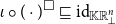 $\iota \circ {(\cdot)}^\Box \sqsubseteq {\text{id}}_{{\mathbb{K}}{{\mathbb{R}}^n_\bot}}$
, and
 ${(\cdot)}^\Box \circ \iota = {\text{id}}_{{\mathbb{I}}{\mathbb{R}}^n_\bot}$
. Therefore,
 $(\iota, {(\cdot)}^\Box)$
forms a continuous embedding-projection pair.
A straightforward modification of the arguments presented so far implies the following variant of Corollary 2.18, formulated for the restricted variants of
 ${\mathbb{I}}{\mathbb{R}}^n_\bot$
and
 ${\mathbb{K}}{{\mathbb{R}}^n_\bot}$
:
Proposition 2.19. For every
 $n \geq 1$
and
 $K \geq 0$
,
 ${\mathbb{I}}{[{-}K,K]^n}$
is a sub-domain of
 ${\mathbb{K}}{[{-}K,K]^n}$
.
Proof. The proof is similar to that of Corollary 2.18, except that the hyperbox closure of (4) must be reformulated as:
 \begin{equation*} \forall C \in {\mathbb{K}}{[{-}K,K]^n}: \quad {C}^\Box := \bigsqcup{\{{R \in {\mathbb{I}}{[{-}K,K]^n}}\mid{C \subseteq R}\}}, \end{equation*}
and, in the other direction, the embedding
 $\iota : {\mathbb{I}}{[{-}K,K]^n} \to {\mathbb{K}}{[{-}K,K]^n}$
defined by
 $\forall x \in {\mathbb{I}}{[{-}K,K]^n}: \iota( x) := x$
must be considered.
Definition 2.20. (Extension, Canonical Interval Extension
 ${If}$
, Approximation).
-
(i) A map
$u: {\mathbb{K}}{{\mathbb{R}}^n_\bot} \to {\mathbb{K}}{{\mathbb{R}}^m_\bot}$
is said to be an extension of
$f: {\mathbb{R}}^n \to {\mathbb{R}}^m$
iff
$\forall x \in {\mathbb{R}}^n: u(\left\{{x}\right\}) = \left\{{f(x)}\right\}$
. -
(ii) A map
$u: {\mathbb{I}}{\mathbb{R}}^n_\bot \to {\mathbb{I}}{\mathbb{R}}^m_\bot$
is said to be an interval extension of
$f: {\mathbb{R}}^n \to {\mathbb{K}}{{\mathbb{R}}^m_\bot}$
iff
$\forall x \in {\mathbb{R}}^n: u(\left\{{x}\right\}) = {f(x)}^\Box$
. -
(iii) For any
$f : {\mathbb{R}}^n \to {\mathbb{K}}{{\mathbb{R}}^m_\bot}$
, we define the canonical interval extension
${If} : {\mathbb{I}}{\mathbb{R}}^n_\bot \to {\mathbb{I}}{\mathbb{R}}^m_\bot$
by: (6) -
(iv) A map
$u: {\mathbb{I}}{\mathbb{R}}^n_\bot \to {\mathbb{I}}{\mathbb{R}}^m_\bot$
is said to be an interval approximation of
$f: {\mathbb{R}}^n \to {\mathbb{K}}{{\mathbb{R}}^m_\bot}$
if
$u \sqsubseteq {If}$
.


Proposition 2.21. For every Euclidean-Scott-continuous
 $f : {\mathbb{R}}^n \to {\mathbb{K}}{{\mathbb{R}}^m_\bot}$
, the canonical interval extension
 ${If}$
defined in (6) is the maximal extension of f among all the extensions in the continuous domain
 ${\mathbb{I}}{\mathbb{R}}^n_\bot \Rightarrow {\mathbb{I}}{\mathbb{R}}^m_\bot$
. In particular,
 ${If}$
is Scott-continuous.
Proof. Given a map
 $f : {\mathbb{R}}^n \to {\mathbb{K}}{{\mathbb{R}}^m_\bot}$
, we define
 ${f}^\Box: {\mathbb{R}}^n \to {\mathbb{I}}{\mathbb{R}}^m_\bot$
by
 ${f}^\Box := {(\cdot)}^\Box \circ f$
, i.e.,
 $\forall x \in {\mathbb{R}}^n: {f}^\Box(x) = {f(x)}^\Box$
. If f is Euclidean-Scott-continuous, then, by Corollary 2.17, so is
 ${f}^\Box$
. It is straightforward to verify that a map
 $u: {\mathbb{I}}{\mathbb{R}}^n_\bot \Rightarrow {\mathbb{I}}{\mathbb{R}}^m_\bot$
is an interval approximation of f if and only if it is an interval approximation of
 ${f}^\Box$
. Thus, it suffices to prove the proposition for the special case of
 $f: {\mathbb{R}}^n \to {\mathbb{I}}{\mathbb{R}}^m_\bot$
.
Footnote 2
This, however, is an immediate consequence of Escardó (Reference Escardó1998, Theorem 4.5.3), because
 ${\mathbb{I}}{\mathbb{R}}^m_\bot$
is a continuous
 -semilattice with unit, for any
 $m \in {\mathbb{N}}$
.
Remark 2.22. Bounded-complete continuous domains are characterized topologically as densely injective
 $T_0$
-spaces. A
 $T_0$
-space Z is said to be densely injective iff it satisfies the following condition for any pair of
 $T_0$
-spaces X and Y, and topological embedding
 $j: X \to Y$
that embeds X as a dense sub-space into Y:
Any continuous map
$f: X \to Z$
has a continuous extension
$f^*: Y \to Z$
satisfying
$f = f^* \circ j$
.


It turns out that bounded-complete continuous domains (equipped with the Scott topology) are exactly densely injective
 $T_0$
-spaces (Gierz et al., Reference Gierz, Hofmann, Keimel, Lawson, Mislove and Scott2003, Proposition II-3.11). Furthermore, when Z is a bounded-complete continuous domain, the function
 $f^*: Y \to Z$
defined by formula (7) below is a continuous extension of f to Y and is indeed the supremum of all such extensions (Gierz et al., Reference Gierz, Hofmann, Keimel, Lawson, Mislove and Scott2003, Proposition II-3.9):

In case Z is a continuous
 -semilattice with unit – of which
 ${\mathbb{K}}{{\mathbb{R}}^m_\bot}$
and
 ${\mathbb{I}}{\mathbb{R}}^m_\bot$
are two instances – and the map j satisfies a fairly mild condition (i.e., j is finitary, Escardó Reference Escardó1998, Definition 2.7.1) then (7) can be simplified to:

in which
 $\uparrow \alpha := \{{y \in Y}\mid{\alpha \sqsubseteq y}\}$
(Escardó, Reference Escardó1998, Theorem 4.5.3). Here,
 $\alpha \sqsubseteq y$
denotes the specialization order defined by
 $\alpha \sqsubseteq y \Longleftrightarrow \forall U \in \Omega(Y): \left( \alpha \in U \implies y \in U \right)$
, i.e., whenever an open set U contains
 $\alpha$
, it must also contain y. When
 $Y={\mathbb{I}}{\mathbb{R}}^n_\bot$
with the Scott topology, the specialization order on Y is the reverse inclusion order of the current article, i.e.,
 $\forall \alpha, y \in {\mathbb{I}}{\mathbb{R}}^n_\bot: \left( \alpha \sqsubseteq y \Longleftrightarrow y \subseteq \alpha \right)$
.
Taking
 $Z = {\mathbb{I}}{\mathbb{R}}^m_\bot$
, and defining
 $j : {\mathbb{R}}^n \to {\mathbb{I}}{\mathbb{R}}^n_\bot$
as
 $\forall x \in {\mathbb{R}}^n: j(x) := \left\{{x}\right\}$
, it can be shown that j is indeed finitary, and clearly, formula (6) can be obtained from (8). Furthermore, the very map
 $f \mapsto {If}$
from
 $({\mathbb{R}}^n \Rightarrow {\mathbb{I}}{\mathbb{R}}^m_\bot)$
to
 $({\mathbb{I}}{\mathbb{R}}^n_\bot \Rightarrow {\mathbb{I}}{\mathbb{R}}^m_\bot)$
is a Scott continuous sub-space embedding (Escardó, Reference Escardó1998, Theorem 4.5.6).
As the restriction of the Scott topology of
 ${\mathbb{K}}{{\mathbb{R}}^m_\bot}$
over
 ${\mathbb{R}}^m$
is the Euclidean topology, we may consider any continuous map
 $f: {\mathbb{R}}^n \to {\mathbb{R}}^m$
also as a function of type
 ${\mathbb{R}}^n \to {\mathbb{K}}{{\mathbb{R}}^m_\bot}$
, and construct its canonical interval extension accordingly, which will be Scott-continuous.
Remark 2.23. The distinction between extension and approximation is crucial in the current article.
3. Global Robustness Analysis
A domain-theoretic framework for abstract robustness analysis was introduced by Moggi et al. (Reference Moggi, Farjudian, Duracz and Taha2018). The essence of the framework is in the link between robustness – a concept defined based on perturbations – and Scott topology – a concept defined in terms of order theory.
Assume that
 ${\mathbb{S}}$
is a metric space,
 ${\mathbb{K}}{{\mathbb{S}}}$
is the pointed dcpo of non-empty compact subsets of
 ${\mathbb{S}}$
, ordered under reverse inclusion, with
 ${\mathbb{S}}$
added as the bottom element if
 ${\mathbb{S}}$
is not compact. When
 ${\mathbb{S}}$
is a compact metric space – which is the relevant case in our discussion – the pointed dcpo
 ${\mathbb{K}}{{\mathbb{S}}}$
becomes an
 $\omega$
-continuous domain (Edalat, Reference Edalat1995b, Proposition 3.4). For each
 $X \subseteq {\mathbb{S}}$
, let
 $\uparrow\negthickspace{X} := \{{C \in {\mathbb{K}}{{\mathbb{S}}}}\mid{C\subseteq X}\}$
. The robust topology is defined over
 ${\mathbb{K}}{{\mathbb{S}}}$
. Intuitively, we regard a collection
 $U \subseteq {\mathbb{K}}{{\mathbb{S}}}$
of compact subsets of
 ${\mathbb{S}}$
as robust open if U is closed under sufficiently small perturbations. Formally, we say that
 $U \subseteq {\mathbb{K}}{{\mathbb{S}}}$
is robust open iff
 $ \forall C \in U : \exists \delta > 0 : \uparrow\negthickspace{B(C,\delta)}\subseteq U$
, in which
 $B(C,\delta)$
is as defined in (2). This topology indeed captures the notion of robustness (Moggi et al., Reference Moggi, Farjudian, Duracz and Taha2018, Theorem A.2). Thus, we define:
Definition 3.1. (Robust Map). Assume that
 ${\mathbb{S}}_1$
and
 ${\mathbb{S}}_2$
are compact metric spaces. We say that
 $f : {\mathbb{K}}{{\mathbb{S}}_1} \to {\mathbb{K}}{{\mathbb{S}}_2}$
is robust iff it is continuous with respect to the robust topologies on
 ${\mathbb{K}}{{\mathbb{S}}_1}$
and
 ${\mathbb{K}}{{\mathbb{S}}_2}$
.
Theorem 3.2. (Moggi et al. Reference Moggi, Farjudian, Duracz and Taha2018, Theorem A.4). For any compact metric space
 ${\mathbb{S}}$
, the Scott and robust topologies on
 ${\mathbb{K}}{{\mathbb{S}}}$
coincide.
Assume that the function
 $N : {\mathbb{S}}_1 \to {\mathbb{S}}_2$
is (the semantic model of) a neural network, and define the reachability map
 $A_N : {\mathbb{K}}{{\mathbb{S}}_1} \to {\mathbb{K}}{{\mathbb{S}}_2}$
as follows:
 \begin{equation} \forall X \in {\mathbb{K}}{{\mathbb{S}}_1}: \quad A_N(X) := \bigcap \{{C \in {\mathbb{K}}{{\mathbb{S}}_2}}\mid{N(X) \subseteq C}\}.\end{equation}
The map
 $A_N$
is clearly monotonic, that is,
 $\forall X, Y \in {\mathbb{K}}{{\mathbb{S}}_1}: X \subseteq Y \implies A_N(X)\subseteq A_N(Y)$
. In case
 $A_N$
is not robust, a valid question is whether it is possible to approximate
 $A_N$
with a robust map without losing too much accuracy. For compact metric spaces, the answer is affirmative:
Corollary 3.3. If
 ${\mathbb{S}}_1$
and
 ${\mathbb{S}}_2$
are compact metric spaces, then any monotonic map
 $f : {\mathbb{K}}{{\mathbb{S}}_1} \to {\mathbb{K}}{{\mathbb{S}}_2}$
has a “tightest” robust approximation
 $f^\circledcirc : {\mathbb{K}}{{\mathbb{S}}_1} \to {\mathbb{K}}{{\mathbb{S}}_2}$
satisfying:
 \begin{equation} \forall X \in {\mathbb{K}}{{\mathbb{S}}_1}: \quad f^\circledcirc(X) = \bigsqcup \{{f(b)}\mid{ b \ll X}\}, \end{equation}
which by Theorem 3.2 must be Scott-continuous. Here, by the tightest we mean the largest under the pointwise ordering of functions.
Proof. The existence of a tightest robust approximation follows from Moggi et al. (Reference Moggi, Farjudian, Duracz and Taha2018, Corollaries 4.4 and 4.5). The formulation (10) follows from Moggi et al. (Reference Moggi, Farjudian, Duracz and Taha2018, Theorem 5.20).
In a typical application, the input space of a neural network is a bounded region of some Euclidean space. Therefore, we consider feedforward neural networks with input space
 $[{-}M,M]^n$
, for some
 $M>0$
. For the output, we will mainly focus on the regressors of type
 $N : [{-}M,M]^n \to {\mathbb{R}}$
. The reason is that, within the framework that we have adopted, robustness analysis of classifiers reduces to Lipschitz estimation of regressors. Assume that
 $\hat{N}: [{-}M,M]^n \to \left\{{c_1, \ldots, c_k}\right\}$
is a classifier network. A common architecture for such a classifier comprises a regressor
 $N \equiv (N_1, \ldots, N_k): [-M,M]^n \to {\mathbb{R}}^k$
followed by an
 $\arg \max$
operation. Thus, for a given input
 $x_0 \in [-M,M]^n$
, the index of the class predicted by
 $\hat{N}$
is
 $i_0 = \arg \max_{1 \leq i \leq k} N_i(x_0)$
. In certified local robustness analysis, the aim is to provide a radius
 $\beta > 0$
such that, for any point x in the neighborhood of radius
 $\beta$
around
 $x_0$
, we have
 $\hat{N}(x) = \hat{N}(x_0)$
, i.e., a neighborhood within which no adversarial examples can be found. A lower bound for such a radius can be obtained by estimating the Lipschitz constants of the functions
 $\{{ N_{i_0} - N_i}\mid{ 1 \leq i \leq k, i \neq i_0}\}$
. As such, robustness analysis of classifiers reduces to Lipschitz estimation of regressors with one output. For more details, the reader may refer to Weng et al. (Reference Weng, Zhang, Chen, Song, Hsieh, Boning, Dhillon and Daniel2018b, Section 3).
When
 $N: [{-}M,M]^n \to {\mathbb{R}}$
is a continuous function – which is the relevant case in our discussion – the image of the compact set
 $[{-}M,M]^n$
will also be compact, which we may assume to be included in a compact interval
 $[{-}M',M']$
, for
 $M' \geq 0$
large enough. Furthermore, the reachability map
 $A_N$
of (9) satisfies
 $\forall X \in {\mathbb{K}}{[{-}M,M]^n}: A_N(X) = N(X)$
.
Before focusing on regressors, however, we briefly discuss some issues related to robustness analysis of classifiers.
3.1 Classifiers
Let
 $C = \left\{{c_1, \ldots, c_k}\right\}$
be a set of classes, with
 $k \geq 1$
, and assume that the function
 $N: [{-}M,M]^n \to C$
is (the semantic model of) a classifier. As C is discrete, it is natural to metrize C using the discrete metric:
 \begin{equation*} \forall x,y \in C: \quad d(x,y) := \left\{ \begin{array}{l@{\quad}l} 0, & \text{if } x = y,\\ 1, & \text{if } x \neq y.\\ \end{array} \right.\end{equation*}
The main problem with a classifier of type
 $N : [{-}M,M]^n \to C$
is the mapping of a connected space to a discrete one, where the topology on
 $[{-}M,M]^n$
is the Euclidean topology, and the topology on C is the discrete topology:
Proposition 3.4. A classifier
 $N: [{-}M,M]^n \to C$
is continuous iff N is constant.
Proof. The
 $\Leftarrow$
direction is obvious. For the
 $\Rightarrow$
direction, as C is a discrete space, then each singleton
 $\left\{{c_i}\right\}$
is an open set. If N is continuous, then each inverse image
 $N^{-1}(c_i)$
must also be open. If N takes more than one value, then
 $[{-}M,M]^n = \bigcup_{1 \leq i \leq k} N^{-1}(c_i)$
must be the union of at least two disjoint non-empty open sets, which is impossible as
 $[{-}M,M]^n$
is a connected space.
Proposition 3.4 implies that a classifier may not be computable – in the framework of TTE (Weihrauch, Reference Weihrauch2000) – unless if it is constant. This is because, by Ko (Reference Ko1991, Theorem 2.13), if N is computable, then it must be continuous.
By moving to compact subsets, however, it is possible to obtain tight robust approximations of classifiers, even in the presence of discontinuities. As C is a finite set, it is compact under the discrete topology, and
 ${\mathbb{K}}{C}$
is the set of non-empty subsets of C, ordered under reverse inclusion.
Theorem 3.5. Assume that
 $A_N : {\mathbb{K}}{[{-}M,M]^n} \to {\mathbb{K}}{C}$
is the reachability map for a classifier
 $N: [{-}M,M]^n \to C$
, defined in (9). Then,
 $A_N$
has a tightest robust approximation
 $A_N^\circledcirc : {\mathbb{K}}{[{-}M,M]^n} \to {\mathbb{K}}{C}$
which is also Scott-continuous.
Proof. Since both
 $[{-}M,M]^n$
and C are compact, the result follows from Corollary 3.3.
Example 3.6. Assume that the classifier
 $N: [{-}1,1] \to \left\{{c_1, c_2}\right\}$
satisfies:
 \begin{equation*} \forall x \in [{-}1,1]: \quad N(x) = \left\{ \begin{array}{l@{\quad}l} c_1, & \text{if } x \in [{-}1,0],\\ c_2, & \text{if } x \in (0,1].\\ \end{array} \right. \end{equation*}
Then, according to (9), we have:
 \begin{equation*} \forall x \in [{-}1,1]: \quad A_N(\left\{{x}\right\}) = \left\{ \begin{array}{l@{\quad}l} \left\{{c_1}\right\}, & \text{if } x \in [{-}1,0],\\ \left\{{c_2}\right\}, & \text{if } x \in (0,1],\\ \end{array} \right. \end{equation*}
while according to (10), we must have:
 \begin{equation*} \forall x \in [{-}1,1]: \quad A_N^\circledcirc(\left\{{x}\right\}) = \left\{ \begin{array}{l@{\quad}l} \left\{{c_1}\right\}, & \text{if } x \in [{-}1,0),\\ \left\{{c_1,c_2}\right\}, & \text{if } x = 0,\\ \left\{{c_2}\right\}, & \text{if } x \in (0,1].\\ \end{array} \right. \end{equation*}
As can be seen from Example 3.6, the tightest robust approximation of a non-constant classifier may be multivalued over certain parts of the input domain.
Theorem 3.7. Assume that
 $N: [{-}M,M]^n \to C$
is a non-constant classifier, and let
 $\hat{N}: {\mathbb{K}}{[{-}M,M]^n} \to {\mathbb{K}}{C}$
be any robust approximation of the reachability map
 $A_N$
. Then,
 $\hat{N}(\left\{{x}\right\})$
must be multivalued for some
 $x \in [{-}M,M]^n$
.
Proof. To obtain a contradiction, assume that
 $\hat{N}(x)$
is single-valued for all
 $x \in [{-}M,M]^n$
. Therefore, the restriction of
 $\hat{N}$
over
 $[{-}M,M]^n$
– which is the set of maximal elements of
 ${\mathbb{K}}{[{-}M,M]^n}$
– must be equal to N. By Corollary 2.11, the classifier
 $N : [{-}M,M]^n \to C$
must be continuous, which, combined with Proposition 3.4, implies that N is a constant classifier, which is a contradiction.
In Theorem 3.7, assume that
 $C = \left\{{c_1, \ldots, c_k}\right\}$
. In case
 $\hat{N}$
is the tightest robust approximation
 $A_N^\circledcirc$
of
 $A_N$
, then
 $\hat{N}$
is required to be multivalued only over the boundaries of
 $N^{-1}(c_1), \ldots, N^{-1}(c_k)$
. In typical applications, these boundaries have Lebesgue measure zero, and the restriction of
 $A_N^\circledcirc$
over
 $[{-}M,M]^n$
is single-valued and equal to N, almost everywhere, e.g., as in Example 3.6. Computability of
 $A_N^\circledcirc$
, however, is an open problem in general (Moggi et al., Reference Moggi, Farjudian, Duracz and Taha2018, Reference Moggi, Farjudian, Taha, Margaria, Graf and Larsen2019a, b), and even in cases where it is known to be computable, little is known about complexity of its computation (Farjudian and Moggi, Reference Farjudian and Moggi2022). Thus, in practice, one aims for robust approximations
 $\hat{N}$
that are “sufficiently” tight, and over
 $[{-}M,M]^n$
, may be multivalued on sets that are not Lebesgue measure zero.
3.2 Regressors
Assume that a given feedforward regressor
 $N: [{-}M,M]^n \to {\mathbb{R}}$
has H hidden layers. We let
 $n_0 := n$
, and for each
 $1 \leq i \leq H$
, let
 $n_i$
denote the number of neurons in the i-th layer. Then, for each
 $1 \leq i \leq H$
, we represent:
the weights as a matrix
$W_i$
, with
$\dim(W_i) = n_i \times n_{i-1}$
;-
the biases as a vector
$b_i$
, with
$\dim(b_i) = n_i \times 1$
; -
and the activation function (seen as a vector field) by
$\sigma_i: {\mathbb{R}}^{n_i} \to {\mathbb{R}}^{n_i}$
.


From the last hidden layer to the single output neuron, the weights are represented as the vector
 $W_{H+1}$
, with
 $\dim(W_{H+1}) = 1 \times n_H$
, and there are no biases or activation functions. For any input
 $x \in [{-}M,M]^n$
, the output of the neural network may be calculated layer-by-layer as follows:
 \begin{equation} \left\{ \begin{array}{l@{\quad}l} Z_0( x) = x,\\ \hat{Z}_i(x) = W_i Z_{i-1}(x) + b_i, & (1 \leq i \leq H),\\ Z_i(x) = \sigma_i \left(\hat{Z}_i(x) \right), & (1 \leq i \leq H),\\ N(x) = W_{H+1} Z_H (x). \end{array} \right.\end{equation}
We let
 ${\mathcal F}$
denote the class of feedforward networks with a single output neuron and Lipschitz continuous activation functions, whose output may be described using (11). Each
 $N \in {\mathcal F}$
is continuous. Hence, it maps the compact set
 $[{-}M,M]^n$
to a compact set, which we assume is included in
 $[{-}M',M']$
, for M’ large enough.
Proposition 3.8. Assume that
 $N: [{-}M,M]^n \to [{-}M',M']$
is a regressor in
 ${\mathcal F}$
, and
 $A_N$
is its reachability map. Then, the map
 $A_N$
has a tightest robust approximation which is a robust extension of N, i.e., an extension according to Definition 2.20 (i).
Proof. Since both
 $[{-}M,M]^n$
and
 $[{-}M',M']$
are compact, by Corollary 3.3, the reachability map
 $A_N$
has a tightest robust approximation
 $A_N^\circledcirc: {\mathbb{K}}{[{-}M,M]^n} \to {\mathbb{K}}{[{-}M',M']}$
. To prove that
 $A_N^\circledcirc$
is indeed an extension of N, we must show that over the maximal elements of
 ${\mathbb{K}}{[{-}M,M]^n}$
, the map
 $A_N^\circledcirc$
takes singleton values. This is a straightforward consequence of the fact that N is continuous.
This is in contrast with the case of classifiers, where the network itself did not have to be even continuous, and we had to be content with tightest robust approximations.
Of particular interest is the interval enclosure of a given regressor, which may not be the tightest robust extension of the regressor, but it is a robust extension nonetheless, which is commonly used in interval analysis of neural networks:
Theorem 3.9. Let
 $N: [{-}M,M]^n \to [{-}M',M']$
be a regressor in
 ${\mathcal F}$
, and assume that:
-
${(\cdot)}^\Box : {\mathbb{K}}{[{-}M,M]^n} \to {\mathbb{I}}{[{-}M,M]^n}$
is the hyperbox closure map of (4).
-
$\tilde{N}: {\mathbb{I}}{[{-}M,M]^n} \to {\mathbb{I}}{[{-}M',M']}$
is any Scott-continuous extension of N, e.g., the canonical interval extension of Definition 2.20 (iii).
-
$\iota : {\mathbb{I}}{[{-}M',M']} \to {\mathbb{K}}{[{-}M',M']}$
is the embedding of the sub-domain
${\mathbb{I}}{[{-}M',M']}$
into
${\mathbb{K}}{[{-}M',M']}$
, as in Proposition 2.19.


Then, the map
 $\hat{N}: {\mathbb{K}}{[{-}M,M]^n} \to {\mathbb{K}}{[{-}M',M']}$
defined by
 $\forall X \in {\mathbb{K}}{[{-}M,M]^n}: \hat{N}(X) := \iota(\tilde{N}({X}^\Box))$
is a robust extension of N.
Proof. We know that
 ${(\cdot)}^\Box$
,
 $\tilde{N}$
, and
 $\iota$
are Scott-continuous. Therefore, the map
 $\hat{N}$
– being a composition of the three – is Scott-continuous. Since both
 $[{-}M,M]^n$
and
 $[{-}M',M']$
are compact, by Theorem 3.2, the map
 $\hat{N}$
is robust. Hence,
 $\hat{N}$
is a robust approximation of N. To prove that
 $\hat{N}$
is a robust extension of N, we must show that over maximal input values it returns singletons. But this is again a straightforward consequence of continuity of N.
4. Validated Local Robustness Analysis
The results of Section 3 concern globally robust approximation of neural networks. In the machine learning literature, robustness analysis is mainly carried out locally, that is, over specific locations in the input domain. A classifier
 $N: {\mathbb{R}}^n \to \left\{{c_1, \ldots, c_k}\right\}$
may be regarded as robust at
 $v \in {\mathbb{R}}^n$
if, for some neighborhood
 $B( \left\{{v}\right\}, r_0)$
of radius
 $r_0 > 0$
, we have:
 $\forall x \in B(\left\{{v}\right\},r_0): N(x) = N(v)$
. In the current article, by attack-agnostic robustness measurement we mean obtaining a tight lower bound for the largest such
 $r_0$
. This, in turn, can be reduced to obtaining a tight upper bound for the local Lipschitz constant in a neighborhood of the point v (Hein and Andriushchenko,Reference Hein and Andriushchenko2017; Weng et al., Reference Weng, Zhang, Chen, Song, Hsieh, Boning, Dhillon and Daniel2018b), which is the focus of the rest of the current article.
From a theoretical angle, the more challenging networks for Lipschitz analysis are those with non-differentiable activation functions, such as
 ${\mathrm{ReLU}}$
. For such functions, a generalized notion of gradient must be used, e.g., the Clarke-gradient (Clarke, Reference Clarke1990). Indeed, the Clarke-gradient has been used recently for robustness analysis of Lipschitz neural networks (Jordan and Dimakis, Reference Jordan and Dimakis2020, Reference Jordan, Dimakis, Meila and Zhang2021). On the other hand, the domain-theoretic L-derivative (Definition 4.4 on page 18) introduced by Edalat (Reference Edalat2008) also coincides with the Clarke-gradient, a fact which was proven for finite-dimensional Banach spaces by Edalat (Reference Edalat2008), and later generalized to infinite-dimensional Banach spaces by Hertling (Reference Hertling2017). Using this, we develop a domain-theoretic framework for Lipschitz analysis of feedforward networks, which provides a theoretical foundation for methods such as Jordan and Dimakis (Reference Jordan and Dimakis2020, Reference Jordan, Dimakis, Meila and Zhang2021).
Working with the L-derivative, however, is computationally costly. It requires computation over
 ${\mathbb{C}}{{\mathbb{R}}^n_\bot}$
and involves a rather complicated chain rule (Proposition 4.3). Therefore, we consider a hyperbox approximation of the L-derivative, which we call the
 $\hat{L}$
-derivative (Definition 4.7). This will allow us to work with the relatively simpler domain
 ${\mathbb{I}}{\mathbb{R}}^n_\bot$
and also a much simpler chain rule (Lemma 4.9). Finally, we will move on to computation of the Lipschitz constant of a given regressor, according to the following overall strategy.
Assume that
 $N \in {\mathcal F}$
is a feedforward regressor. By using (11), we obtain a unique closed-form expression for N in terms of the weights, biases, and the activation functions. Let
 $\tilde{L}(N): {\mathbb{I}}{[{-}M,M]^n} \to {\mathbb{I}}{\mathbb{R}}^n_\bot$
denote the interval approximation of the
 $\hat{L}$
-derivative of N obtained by applying the chain rule of Lemma 4.9 over this closed-form expression. The map
 $\tilde{L}(N)$
is Scott-continuous. Since we consider
 ${\left\lVert{.}\right\rVert}_{\infty}$
as the perturbation norm, we must compute the
 ${\left\lVert{.}\right\rVert}_1$
-norm of the gradients (see Remark 2.1). First, we extend addition and the absolute value function to real intervals by defining
 $I+J := \{{x+y}\mid{x \in I \wedge y \in J}\}$
and
 ${\lvert{I}\rvert} := \{{{\lvert{x}\rvert}}\mid{x\in I}\}$
, respectively, for all intervals I and J. Then, we extend the
 ${\left\lVert{.}\right\rVert}_1$
norm to hyperboxes by defining
 ${\left\lVert{\prod_{i=1}^n I_i}\right\rVert}_1 := \sum_{i=1}^n {\lvert{I_i}\rvert}$
. For instance, we have
 ${\left\lVert{[{-}1,1] \times [{-}1,2]}\right\rVert}_1 = [0,1] + [0,2] = [0,3]$
. The function
 ${\left\lVert{.}\right\rVert}_1 : {\mathbb{I}}{\mathbb{R}}^n_\bot \to {\mathbb{I}}{\mathbb{R}}^1_\bot$
is also Scott-continuous. Therefore, the composition
 ${\left\lVert{\tilde{L}(N)}\right\rVert}_1: {\mathbb{I}}{[{-}M,M]^n} \to{\mathbb{I}}{\mathbb{R}}^1_\bot$
is a Scott-continuous function. All that remains is to find the maximum value and the maximum set of
 ${\left\lVert{\tilde{L}(N)}\right\rVert}_1$
to approximate the Lipschitz constant and the set of points where the maximum Lipschitz values are attained, within any given neighborhood. This is one of the main contributions of the current article and will be presented in detail in Section 4.4.
If, instead of
 ${\mathbb{I}}{\mathbb{R}}^n_\bot$
, we use the finer domain
 ${\mathbb{C}}{{\mathbb{R}}^n_\bot}$
, then the suitable chain rule will be that of Proposition 4.3, which provides a more accurate result, at the cost of calculating the closed convex hull. This has also been observed in Jordan and Dimakis (Reference Jordan, Dimakis, Meila and Zhang2021). By using the
 $\hat{L}$
-derivative and the chain rule of Lemma 4.9, we avoid computation of the convex hull and trade some accuracy for efficiency. As it turns out, however, we will not lose any accuracy over general position
 ${\mathrm{ReLU}}$
networks (Theorem 4.19), or over differentiable networks (Theorem 4.21).
Remark 4.1. In this article, we focus on the
 ${\left\lVert{.}\right\rVert}_{\infty}$
-norm for perturbations because we will be working with hyperboxes, and in the implementation, we will use interval arithmetic. This does not mean, however, that we cannot analyze robustness with respect to
 ${\left\lVert{.}\right\rVert}_p$
for other values of p. For example, assume that we are given a closed neighborhood
 $V(x_0,r) := \{{x \in {\mathbb{R}}^n}\mid{ {\left\lVert{x - x_0}\right\rVert}_p \leq r}\}$
, for some
 $p \in [1, \infty)$
. We can first cover the neighborhood
 $V(x_0,r)$
with (a large number of sufficiently small) hyperboxes
 $B = \{{b_i}\mid{i \in I}\}$
. We obtain an overapproximation of the
 ${\left\lVert{.}\right\rVert}_{p'}$
-norm of the Clarke-gradient over each box
 $b_i$
and then obtain an approximation of the Lipschitz constant over the neighborhood
 $V(x_0,r)$
.
4.1 Lipschitz continuity and Lipschitz constant
Assume that
 $(X, \delta_X)$
and
 $(Y, \delta_Y)$
are two metric spaces,
 $f : X \to Y$
, and
 $A \subseteq X$
. A real number
 $L \geq 0$
is said to be a Lipschitz bound for f over A if:
 \begin{equation} \forall a, b \in A: \delta_Y(f(a), f(b)) \leq L \delta_X( a, b).\end{equation}
A function for which such a bound exists is said to be Lipschitz continuous over A, and the smallest L satisfying (12) – which must exist – is called the Lipschitz constant of f over A.
If f is Lipschitz continuous over A, then it is also continuous over A, although the converse is not true. For instance, the function
 $h : \ell^1_\infty \to \ell^1_\infty$
, defined by
 $h(x) := \sqrt{{\lvert{x}\rvert}}$
, is continuous everywhere, but not Lipschitz continuous over any neighborhood of 0. Whenever X is a compact subset of
 $\ell^n_\infty$
and
 $f: X \to {\mathbb{R}}$
is continuously differentiable, then f is Lipschitz over X, but again, the converse is not true. For example, the function
 $h: [{-}1,1] \to {\mathbb{R}}$
, defined by
 $h(x) := {\lvert{x}\rvert}$
, is Lipschitz continuous, but not differentiable at 0. To summarize, we have the following inclusions for functions over compact subsets of
 ${\mathbb{R}}^n$
:
 \begin{equation*} \text{Continuously Differentiable} \subset \text{Lipschitz Continuous} \subset \text{Continuous}.\end{equation*}
Even though the inclusions are strict, there is a close relationship between Lipschitz continuity and differentiability. Rademacher’s theorem states that if f is Lipschitz continuous over an open subset A of
 ${\mathbb{R}}^n$
, then it is (Fréchet) differentiable almost everywhere (with respect to the Lebesgue measure) over A (Clarke et al., Reference Clarke, Ledyaev, Stern and Wolenski1998, Corollary 4.19). For example, the function
 ${\mathrm{ReLU}}$
– defined by
 $\forall x \in {\mathbb{R}}: {\mathrm{ReLU}}(x) := \max( 0, x)$
– is (classically) differentiable everywhere except at zero:
 \begin{equation*} ({\mathrm{ReLU}})'(x) = \left\{ \begin{array}{l@{\quad}l} 1, & \text{if } x > 0, \\ 0, & \text{if } x < 0, \\ \mathrm{undefined}, & \text{if } x = 0. \end{array} \right.\end{equation*}
4.2 Clarke-gradient
Although
 ${\mathrm{ReLU}}$
is not differentiable at 0, one-sided limits of the derivative exist, i.e.,:
 \begin{equation} \lim_{x \to 0^-} ({\mathrm{ReLU}})'(x) = 0 \quad \text{and} \quad \lim_{x \to 0^+} ({\mathrm{ReLU}})'(x) = 1.\end{equation}
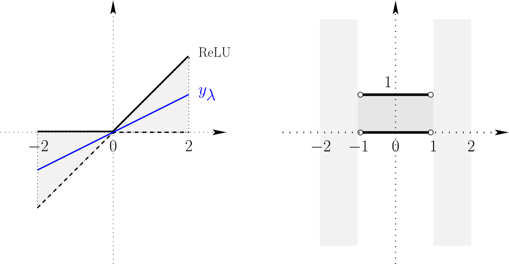
As shown in Figure 1 (Left), in geometric terms, for every
 $\lambda \in [0,1]$
, the line
 $y_\lambda(x) := \lambda x$
satisfies:
 \begin{equation} y_\lambda (0) = {\mathrm{ReLU}} (0) \quad \wedge \quad \forall x \in {\mathbb{R}}: y_\lambda(x) \leq {\mathrm{ReLU}} (x).\end{equation}
The interval [0, 1] is the largest set of
 $\lambda$
values which satisfy (14) and may be considered as a gradient set for
 ${\mathrm{ReLU}}$
at zero. The concept of generalized (Clarke) gradient formalizes this idea. The Clarke-gradient may be defined for functions over any Banach space X (Clarke, Reference Clarke1990, p. 27). When X is finite-dimensional, however, the Clarke-gradient of
 $f: X \to {\mathbb{R}}$
has a simpler characterization. Assume that X is an open subset of
 ${\mathbb{R}}^n$
, and
 $f: X \to {\mathbb{R}}$
is Lipschitz continuous over X. By Rademacher’s theorem, we know that the set
 ${\mathcal N}_f := \{{z \in X}\mid{f \text{ is not differentiable at } z \, }\}$
has Lebesgue measure zero. The Clarke-gradient
 $\partial{f}(x)$
of f at any
 $x \in X$
satisfies:

Equation (15) should be interpreted as follows: take any sequence
 $(x_i)_{i \in {\mathbb{N}}}$
, which completely avoids the set
 ${\mathcal N}_f$
of points where f is not differentiable, converges to x, and for which
 $\lim_{i \to \infty} \nabla f(x_i)$
exists. The Clarke-gradient is the convex hull of these limits (Clarke, Reference Clarke1990, p. 63). It should be clear from (13) and (15) that
 $\partial{{\mathrm{ReLU}}}(0) = [0,1]$
.
Left: The function
 ${\mathrm{ReLU}}: (-2,2) \to {\mathbb{R}}$
(solid black) and the line
 $y_\lambda$
(in
 ) from (14) for some
 $\lambda \in [0,1]$
, which lies entirely in the shaded cone. Right: The step function
 $b \chi_O: (-2,2) \to {\mathbb{I}}{\mathbb{R}}_\bot$
in which
 $b = [0,1]$
and
 $O = (-1,1)$
. We have
 ${\mathrm{ReLU}} \in \delta(O,b)$
.

Proposition 4.2. (Clarke Reference Clarke1990, Proposition 2.1.2). Assume that
 $p \in [1,\infty]$
. Let X be an open subset of
 $\ell^n_p$
and
 $f: X \to {\mathbb{R}}$
be Lipschitz continuous over X with a Lipschitz bound L. Then, for every
 $x \in X$
:
-
(i)
$\partial{f}(x)$
is a non-empty, convex, and compact subset of
${\mathbb{R}}^n$
. -
(ii)
$\forall \xi \in \partial{f}(x): {\left\lVert{\xi}\right\rVert}_{p'} \leq L$
, in which p’ is the conjugate of p as defined in (1).


The following chain rule for the Clarke-gradient is crucial for proving the soundness of methods such as Chaudhuri et al. (Reference Chaudhuri, Gulwani and Lublinerman2012, Reference Chaudhuri, Gulwani, Lublinerman and Navidpour2011), Jordan and Dimakis (Reference Jordan and Dimakis2020, Reference Jordan, Dimakis, Meila and Zhang2021), Laurel et al. (Reference Laurel, Yang, Singh and Misailovic2022):
Proposition 4.3. (Chain Rule, Clarke Reference Clarke1990, Theorem 2.3.9). Assume that
 $X \subseteq {\mathbb{R}}^n$
is open,
 $h = (h_1, \ldots, h_m): X \to {\mathbb{R}}^m$
is Lipschitz continuous in a neighborhood of
 $x \in X$
, and
 $g : {\mathbb{R}}^m \to {\mathbb{R}}$
is Lipschitz continuous in a neighborhood of
 $h(x) \in {\mathbb{R}}^m$
. Then,
 $f := g \circ h$
is Lipschitz in a neighborhood of x, and we have:

in which,
 $\overline{\text{co}}$
denotes the closed convex hull.
Unlike the chain rule for the classical derivative, the chain rule of (16) provides only a subset relation, which, in general, is not an equality. A simple example of lack of equality is shown in Figure 3, which demonstrates an instance of the dependency problem (see Section 4.6.2).
4.3 Domain-theoretic L-derivative
We recall the concept of a domain-theoretic derivative for a function
 $f: U \to {\mathbb{R}}$
defined on an open set
 $U \subseteq {\mathbb{R}}^n$
. Assume that
 $(X, \Omega)$
is a topological space, and
 $(D, \sqsubseteq)$
is a pointed dcpo, with bottom element
 $\bot$
. Then, for any open set
 $O \in \Omega$
, and any element
 $b \in D$
, we define the single-step function
 $b \chi_O: X \to D$
as follows:
 \begin{equation} b \chi_O (x) := \left\{ \begin{array}{l@{\quad}l} b, & \text{if } x \in O,\\ \bot, & \text{if } x \in X \setminus O. \end{array} \right.\end{equation}
Definition 4.4. (L-derivative, Edalat et al. Reference Edalat, Lieutier and Pattinson2013, Section 2). Assume that
 $O \subseteq U \subseteq {\mathbb{R}}^n$
, both O and U are open, and
 $b \in {\mathbb{C}}{{\mathbb{R}}^n_\bot}$
:
-
(i) The single-step tie
$\delta(O, b)$
is the set of all functions
$f : U \to {\mathbb{R}}$
that satisfy
$\forall x, y \in O: b(x-y) \sqsubseteq f(x) - f(y)$
. The set
$b(x-y)$
is obtained by taking the inner product of every element of b with the vector
$x-y$
, and
$\sqsubseteq$
is the reverse inclusion order on
${\mathbb{C}}{{\mathbb{R}}^1_\bot}$
. -
(ii) The L-derivative of any function
$f: U \to {\mathbb{R}}$
is defined as: As such, the map L has type
$$L(f): = \bigsqcup \{ b{\chi _O}|O \subseteq U,b \in _ \bot ^n,f \in \delta (O,b)\} .$$
$L: (U \to {\mathbb{R}}) \to (U \to {\mathbb{C}}{{\mathbb{R}}^n_\bot})$
.


Example 4.5. Assume that
 $U = (-2,2)$
. Consider the function
 ${\mathrm{ReLU}}: (-2,2) \to {\mathbb{R}}$
and the step function
 $b \chi_O: (-2,2) \to {\mathbb{I}}{\mathbb{R}}_\bot$
with
 $b = [0,1]$
and
 $O = (-1,1)$
, as depicted in Figure 1. We have
 ${\mathrm{ReLU}} \in \delta(O,b)$
. In fact, we have
 ${\mathrm{ReLU}} \in \delta(O,b)$
for any open set O containing zero, e.g., the interval
 $(-2^n, 2^n)$
, for any
 $n \in {\mathbb{N}}$
. Thus, one may verify that:
 \begin{equation*} \forall x \in (-2,2): \quad L({\mathrm{ReLU}})(x) = \left\{ \begin{array}{l@{\quad}l} 0, & \text{if } x < 0,\\ {[0,1]}, & \text{if } x = 0,\\ 1, & \text{if } x > 0. \end{array} \right. \end{equation*}
For any
 $f: U \to {\mathbb{R}}$
, the L-derivative
 $L(f): U \to {\mathbb{C}}{{\mathbb{R}}^n_\bot}$
is Euclidean-Scott-continuous. When f is classically differentiable at
 $x \in U$
, the L-derivative and the classical derivative coincide (Edalat, Reference Edalat2008). Many of the fundamental properties of the classical derivative can be generalized to the domain-theoretic one, e.g., additivity and the chain rule (Edalat and Pattinson, Reference Edalat and Pattinson2005). Of particular importance to the current paper is the following result:
Theorem 4.6. (Edalat Reference Edalat2008; Hertling Reference Hertling2017). Over Lipschitz continuous functions
 $f: U \to {\mathbb{R}}$
, the domain-theoretic L-derivative coincides with the Clarke-gradient, i.e.,
 $\forall x \in U: L(f)(x) = \partial{f}(x)$
.
In this paper, instead of working with the general convex sets in
 ${\mathbb{C}}{{\mathbb{R}}^n_\bot}$
, we work with the simpler hyperboxes in
 ${\mathbb{I}}{\mathbb{R}}^n_\bot$
:
Definition 4.7. (
 $\hat{L}$
-derivative). Let
 $U \subseteq {\mathbb{R}}^n$
be an open set. In the definition of L-derivative (Definition 4.4), if
 ${\mathbb{C}}{{\mathbb{R}}^n_\bot}$
is replaced with
 ${\mathbb{I}}{\mathbb{R}}^n_\bot$
, then we obtain the concept of
 $\hat{L}$
-derivative for functions of type
 $U \to {\mathbb{R}}$
. For vector valued functions
 $f = ( f_1, \ldots, f_m): U \to {\mathbb{R}}^m$
, we define:
 \begin{equation*} \hat{L}(f) := \left( \hat{L}(f_1), \ldots, \hat{L}(f_m) \right)^\intercal, \end{equation*}
in which,
 $(\cdot)^\intercal$
denotes the transpose of a matrix. In other words, for each
 $1 \leq i \leq m$
and
 $x \in U$
, let
 $\hat{L}(f_i)(x) \equiv ( \alpha_{i,1}, \ldots, \alpha_{i,n}) \in {\mathbb{I}}{\mathbb{R}}^n_\bot$
. Then, for each
 $x \in U$
,
 $\hat{L}(f)(x)$
is the
 $m \times n$
interval matrix
 $[\alpha_{i,j}]_{1 \leq i \leq m, 1 \leq j \leq n}$
.
The
 $\hat{L}$
-derivative is, in general, coarser than the L-derivative, as the following example demonstrates:
Example 4.8. Let
 $D_n$
denote the closed unit disc in
 ${\mathbb{R}}^n$
, and define
 $f: {\mathbb{R}}^n \to {\mathbb{R}}$
by
 $f(x) = {\left\lVert{x}\right\rVert}_2$
, in which
 ${\left\lVert{\cdot}\right\rVert}_2$
is the Euclidean norm. Then,
 $L(f)(0) = D_n$
, while
 $\hat{L}(f)(0) = [{-}1,1]^n$
.
As such, we lose some precision by using hyperboxes. On the other hand, on hyperboxes, the chain rule has a simpler form:
Lemma 4.9. (Chain Rule on Hyperboxes, Edalat and Pattinson Reference Edalat and Pattinson2005, Lemma 3.3). For any two functions
 $g : {\mathbb{R}}^k \to {\mathbb{R}}^m$
and
 $f: {\mathbb{R}}^m \to {\mathbb{R}}^n$
, we have:
 \begin{equation*} \hat{L}(f)(g(x)) \times \hat{L}(g)(x) \sqsubseteq \hat{L}(f \circ g)(x). \end{equation*}
4.4 Maximization algorithm
For any closed compact interval I, we write
 $I = [\underline{I}, \overline{I}]$
. Assume that
 $f : {\mathbb{R}}^n \to {\mathbb{I}}{\mathbb{R}}^1_\bot$
and
 $X \subseteq {\mathbb{R}}^n$
is a compact set. We define the maximum value and maximum set of f over X as follows:
 $$\left\{ {\matrix{
{{\rm{ma}}{{\rm{x}}_{\rm{V}}}(f,X): = [\underline{z}, \bar z],\quad {\rm{where}}\, \underline{z} : = {{\sup }_{x \in X}}\underline {f(x)} \,{\rm{and}}\,\bar z: = {{\sup }_{x \in X}}\overline {f(x)} } \hfill \cr
{{\rm{ma}}{{\rm{x}}_{\rm{S}}}(f,X): = \{ x \in X|f(x) \cap {\rm{ma}}{{\rm{x}}_{\rm{V}}}(f,X) \ne \emptyset \} .} \hfill \cr } } \right.$$
For any
 $\hat{f}: {\mathbb{I}}{\mathbb{R}}^n_\bot \to {\mathbb{I}}{\mathbb{R}}^1_\bot$
, the maximum value and maximum set are defined by considering the restriction of
 $\hat{f}$
over the maximal elements
 ${\mathbb{R}}^n$
.
Proposition 4.10. Assume that
 $\hat{f}: {\mathbb{I}}{\mathbb{R}}^n_\bot \to {\mathbb{I}}{\mathbb{R}}^1_\bot$
is Scott-continuous, and X is a compact subset of
 ${\mathbb{R}}^n$
. Then
 $\text{max}_{\rm S}(\hat{f},X)$
is a compact subset of
 ${\mathbb{R}}^n$
.
Proof. Let
 $f : {\mathbb{R}}^n \to {\mathbb{I}}{\mathbb{R}}^1_\bot$
be the restriction of
 $\hat{f}$
over the maximal elements
 ${\mathbb{R}}^n$
. As X is compact, it suffices to prove that
 $\text{max}_{\rm S}(f,X)$
is a closed subset of X. Let
 $x \in X \setminus \text{max}_{\rm S}(f,X)$
be an arbitrary point, and write
 $f(x) = [\underline{f(x)}, \overline{f(x)}]$
. Since
 $x \not \in \text{max}_{\rm S}(f,X)$
, then
 $\overline{f(x)} < \underline{z}$
, where
 $z \equiv [\underline{z}, \overline{z}] = \text{max}_{\rm V}(f,X)$
. As
 $\hat{f}$
is Scott-continuous, then, by Corollary 2.11, the map f must be Euclidean-Scott-continuous. In turn, by Proposition 2.14, the function
 $\overline{f}$
must be upper semi-continuous. As
 $\overline{f(x)} < \underline{z}$
, for some neighborhood
 $O_x$
of x, we must have:
 $\forall y \in O_x: \overline{f(y)} < \underline{z}$
. This entails that
 $O_x \cap \text{max}_{\rm S}(f,X) = \emptyset$
.
Thus, in the sequel, we consider the functionals:
 $$\left\{ {\matrix{
{{\rm{ma}}{{\rm{x}}_{\rm{V}}}:\quad (\mathbb{IR}_ \bot ^n \Rightarrow \mathbb{IR}_ \bot ^1) \to \mathbb{KR}_ \bot ^n \to \mathbb{IR}_ \bot ^1,} \hfill \cr
{{\rm{ma}}{{\rm{x}}_{\rm{S}}}:\quad (\mathbb{IR}_ \bot ^n \Rightarrow \mathbb{IR}_ \bot ^1) \to \mathbb{KR}_ \bot ^n \to \mathbb{KR}_ \bot ^n,} \hfill \cr } } \right.$$
which, given any Scott-continuous
 $f \in {\mathbb{I}}{\mathbb{R}}^n_\bot \Rightarrow {\mathbb{I}}{\mathbb{R}}^1_\bot$
and compact set
 $X \in {\mathbb{K}}{{\mathbb{R}}^n_\bot}$
, return the maximum value and the maximum set of f over X, respectively. As an example, assume that
 $f \in {\mathbb{I}}{\mathbb{R}}^1_\bot \Rightarrow {\mathbb{I}}{\mathbb{R}}^1_\bot$
is the canonical interval extension of
 $\partial{{\mathrm{ReLU}}}: {\mathbb{R}} \to {\mathbb{I}}{\mathbb{R}}^1_\bot$
. Then:
 \begin{equation} \left\{ \begin{array}{l@{\quad}l} \text{max}_{\rm V}(f,[{-}1,1]) = [1,1], & \text{max}_{\rm S}(f,[{-}1,1]) = [0,1], \\\text{max}_{\rm V}(f,[{-}1,0]) = [0,1], & \text{max}_{\rm S}(f,[{-}1,0]) = [{-}1,0], \\ \end{array} \right.\end{equation}
which shows that the functionals
 $\text{max}_{\rm V}$
and
 $\text{max}_{\rm S}$
are not even monotone in their second argument. For fixed second arguments, however, both are Scott-continuous in their first argument:
Theorem 4.11. (Scott continuity). For any
 $X \in {\mathbb{K}}{{\mathbb{R}}^n_\bot}$
, the functionals
 $\text{max}_{\rm V}(\cdot , X): ({\mathbb{I}}{\mathbb{R}}^n_\bot \Rightarrow {\mathbb{I}}{\mathbb{R}}^1_\bot) \to {\mathbb{I}}{\mathbb{R}}^1_\bot$
and
 $\text{max}_{\rm S}( \cdot, X): ({\mathbb{I}}{\mathbb{R}}^n_\bot \Rightarrow {\mathbb{I}}{\mathbb{R}}^1_\bot) \to {\mathbb{K}}{{\mathbb{R}}^n_\bot}$
are Scott-continuous.
Proof. As the domains
 ${\mathbb{I}}{\mathbb{R}}^n_\bot \Rightarrow {\mathbb{I}}{\mathbb{R}}^1_\bot$
,
 ${\mathbb{I}}{\mathbb{R}}^1_\bot$
, and
 ${\mathbb{K}}{{\mathbb{R}}^n_\bot}$
are
 $\omega$
-continuous, by Proposition 2.9, it suffices to show that both functionals are monotone and preserve the suprema of
 $\omega$
-chains.
To prove monotonicity, assume that
 $f,g \in {\mathbb{I}}{\mathbb{R}}^n_\bot \Rightarrow {\mathbb{I}}{\mathbb{R}}^1_\bot$
, and
 $f \sqsubseteq g$
. Thus,
 $\forall x \in X: (\underline{f(x)} \leq \underline{g(x)}) \wedge (\overline{g(x)} \leq\overline{f(x)})$
. This implies that
 $\sup_{x \in X} \underline{f(x)} \leq \sup_{x \in X} \underline{g(x)}$
and
 $\sup_{x \in X} \overline{g(x)} \leq \sup_{x \in X} \overline{f(x)}$
. Therefore:
 \begin{equation} \text{max}_{\rm V}(f,X) \sqsubseteq \text{max}_{\rm V}(g,X). \end{equation}
Take an arbitrary
 $x \in \text{max}_{\rm S}(g,X)$
. By definition, we must have
 $g(x) \cap \text{max}_{\rm V}(g,X) \neq \emptyset$
, which, combined with the assumption
 $f \sqsubseteq g$
, implies
 $f(x) \cap \text{max}_{\rm V}(g,X) \neq \emptyset$
. This, combined with (20), entails that
 $f(x) \cap \text{max}_{\rm V}(f,X) \neq \emptyset$
. Hence,
 $x \in \text{max}_{\rm S}(f,X)$
, and we have
 $\text{max}_{\rm S}(f,X) \sqsubseteq \text{max}_{\rm S}(g,X)$
. The proof of monotonicity is complete.
Next, let
 $(f_n)_{n \in {\mathbb{N}}}$
be an
 $\omega$
-chain in
 ${\mathbb{I}}{\mathbb{R}}^n_\bot \Rightarrow {\mathbb{I}}{\mathbb{R}}^1_\bot$
, with
 $f = \bigsqcup_{n \in {\mathbb{N}}} f_n$
. As both
 $\text{max}_{\rm V}$
and
 $\text{max}_{\rm S}$
are monotone, we have
 $\bigsqcup_{n \in {\mathbb{N}}} \text{max}_{\rm V}(f_n,X) \sqsubseteq \text{max}_{\rm V}(f,X)$
and
 $\bigsqcup_{n \in {\mathbb{N}}} \text{max}_{\rm S}(f_n,X) \sqsubseteq \text{max}_{\rm S}(f,X)$
. Thus, it only remains to prove the
 $\sqsupseteq$
direction in both cases. In what follows, we let
 $z \equiv [\underline{z}, \overline{z}] := \text{max}_{\rm V}(f,X)$
, and for each
 $n \in {\mathbb{N}}$
,
 $z_n \equiv [\underline{z_n}, \overline{z_n}] := \text{max}_{\rm V}(f_n,X)$
.
maxV: First, consider an arbitrary
 $t < \underline{z}$
and let
 $\epsilon := (\underline{z}-t)/4$
. By definition,
 $\exists x_0 \in X: \underline{f(x_0)} > \underline{z} - \epsilon$
. Since
 $f = \bigsqcup_{n \in {\mathbb{N}}} f_n$
, we must have
 $\exists N_0 \in {\mathbb{N}}: \forall n \geq N_0: \underline{f_n(x_0)} > \underline{f(x_0)} - \epsilon > \underline{z}- 2\epsilon > t$
. Therefore:
 \begin{equation} \forall t \in {\mathbb{R}}: \quad t < \underline{z} \implies \exists n \in {\mathbb{N}}: t < \underline{z_n}. \end{equation}
Next, we consider an arbitrary
 $t > \overline{z}$
and let
 $\epsilon := (t - \overline{z})/4$
. Since
 $f = \bigsqcup_{n \in {\mathbb{N}}} f_n$
, we must have:
 \begin{equation*} \forall x \in X: \exists N_x \in {\mathbb{N}}: \forall n \geq N_x: \quad \overline{f_n(x)} < \overline{f(x)} + \epsilon. \end{equation*}
For each fixed
 $n \in {\mathbb{N}}$
, the map
 $\overline{f_n}$
is upper semi-continuous. Hence, for any
 $x \in X$
, there exists a neighborhood
 $O_x$
of x for which we have
 \begin{equation*} \forall y \in O_x: \quad \overline{f_{N_x}(y)} < \overline{f_{N_x}(x)} + \epsilon < \overline{f(x)} + 2\epsilon \leq \overline{z} + 2\epsilon. \end{equation*}
As the sequence
 $(f_n)_{n \in {\mathbb{N}}}$
is assumed to be an
 $\omega$
-chain, the upper bounds
 $(\overline{f_n})_{n \in {\mathbb{N}}}$
are non-increasing, and we obtain:
 \begin{equation*} \forall x \in X: \forall y \in O_x: \forall n \geq N_x: \quad \overline{f_n(y)} \leq \overline{z} + 2\epsilon. \end{equation*}
As X is compact and
 $X \subseteq \bigcup_{x \in X} O_x$
, then for finitely many neighborhoods
 $\left\{{O_{x_1}, \ldots, O_{x_m}}\right\}$
we must have
 $X \subseteq \bigcup_{i=1}^m O_{x_i}$
. Thus, if we let
 $N_0 := \max\left\{{N_{x_1}, \ldots, N_{x_m}}\right\}$
, we must have:
 \begin{equation*} \forall n \geq N_0: \forall y \in X: \quad \overline{f_n(y)} \leq \overline{z} + 2\epsilon, \end{equation*}
which entails that:
 \begin{equation} \forall t \in {\mathbb{R}}: \quad \overline{z} < t \implies \exists N_0 \in {\mathbb{N}}: \forall n \geq N_0: \overline{z_n} \leq \overline{z} + 2\epsilon < t. \end{equation}
From (21) and (22), we deduce that
 $\bigsqcup_{n \in {\mathbb{N}}} \text{max}_{\rm V}(f_n,X) \sqsupseteq \text{max}_{\rm V}(f,X)$
.
maxS: Assume that
 $x \in X \setminus \text{max}_{\rm S}(f,X)$
, which implies that
 $\overline{f(x)} < \underline{z}$
. Take
 $\epsilon = \left(\underline{z} - \overline{f(x)}\right)/4$
. Since
 $\underline{z} = \sup_{y \in X} \underline{f(y)}$
, there exists
 $x_1 \in X$
such that
 $\underline{f(x_1)} > \underline{z} - \epsilon$
. As
 $f = \bigsqcup_{n \in {\mathbb{N}}} f_n$
, there exists
 $N_1 \in {\mathbb{N}}$
, such that:
 \begin{equation} \forall n \geq N_1: \underline{f_n(x_1)} > \underline{f(x_1)} - \epsilon > \underline{z} - 2\epsilon. \end{equation}
Furthermore, there exists
 $N_2 \in {\mathbb{N}}$
, such that:
 \begin{equation} \forall n \geq N_2: \overline{f_n(x)} < \overline{f(x)} + \epsilon = \underline{z} - 3\epsilon. \end{equation}
Taking
 $N_3 = \max\left\{{N_1,N_2}\right\}$
, from (23) and (24), we obtain
 $\forall n \geq N_3: \overline{f_n(x)} < \underline{f_n(x_1)} \leq \underline{z_n}$
, which implies that
 $x \not \in \text{max}_{\rm S}(f_n,X)$
. Therefore,
 $\bigsqcup_{n \in {\mathbb{N}}} \text{max}_{\rm S}(f_n,X) \sqsupseteq \text{max}_{\rm S}(f,X)$
.
The proof is complete.
Algorithm 1 presents an implementation of
 $\text{max}_{\rm V}$
and
 $\text{max}_{\rm S}$
, which we use in our experiments. As pointed out before, the set
 $B_{{\mathbb{K}}{{\mathbb{R}}^n_\bot}}$
, consisting of finite unions of rational hyperboxes, forms a countable basis for the
 $\omega$
-continuous domain
 ${\mathbb{K}}{{\mathbb{R}}^n_\bot}$
. We have used this fact in Algorithm 1, which outputs enclosures of the maximum set using elements of
 $B_{{\mathbb{K}}{{\mathbb{R}}^n_\bot}}$
.

Apart from the function f and the neighborhood X, Algorithm 1 requires three other input parameters:
 $m_{\iota}$
,
 $m_b$
, and
 $\delta$
. These are crucial for making sure that the algorithm stops below a reasonable threshold. In line 9, we discard all the boxes in
 $B_i$
which cannot possibly contain any maximum points. How many boxes are discarded depends on a number of factors, most importantly, whether the function f has a flat section around the maximum set or not. The condition
 $2^n{\lvert{\hat{B}_i}\rvert} \geq m_b$
in line 13 is necessary, because in cases where flat sections exist, the number of elements of
 $\hat{B}_i$
grows exponentially with each iteration. In the if statement of line 10, we make sure that bisecting
 $\hat{B}_i$
will not create too many boxes before executing the bisection command in the first place. In the current article, by bisecting a box
 $b \subseteq {\mathbb{R}}^n$
we mean bisecting along all the n coordinates, which generates
 $2^n$
boxes. As such, in line 11 of the algorithm, every box in
 $\hat{B}_i$
is bisected along all the n coordinates, and the result is assigned to
 $B_{i+1}$
. Figure 2 depicts the first three bisections for a scenario in which
 $n=2$
. Note that, due to the overlap of the interval values of the function f in adjacent boxes, when extracting
 $\hat{B}_2$
from
 $B_2$
(which is performed in line 9) no boxes may be discarded, and the earliest that a box may be discarded is when
 $\hat{B}_3$
is extracted from
 $B_3$
.
The dynamics of the first three bisections of Algorithm 1 for a two-dimensional scenario. The starting search region X is shown in blue color for reference.

Algorithm 1 closely follows the definition of
 $\text{max}_{\rm V}$
and
 $\text{max}_{\rm S}$
given in (18). Hence, the proof of soundness is straightforward:
Lemma 4.12. (Soundness). For any given f, X,
 $m_{\iota}$
,
 $m_b$
, and
 $\delta$
, Algorithm 1 halts in finite time and returns enclosures of
 $\text{max}_{\rm V}(f,X)$
and
 $\text{max}_{\rm S}(f,X)$
.
Proof. We prove the lemma by induction over i, that is, the number of iterations of the main repeat-until loop. When
 $i=1$
, we have
 $B_i = X$
, which trivially contains
 $\text{max}_{\rm S}(f, X)$
.
For the inductive step, assume that at iteration i, before the start of the loop, the finite set of hyperboxes
 $B_i$
satisfies
 $\text{max}_{\rm S}(f,X) \subseteq \bigcup B_i$
. Assume that
 $\tilde{f} \in X \Rightarrow {\mathbb{I}}{\mathbb{R}}^1_\bot$
is the restriction of the interval function f over the maximal elements X, which entails that f is an interval approximation of
 $\tilde{f}$
. As a result,
 $I_i$
is an overapproximation of
 $\text{max}_{\rm V}(\tilde{f},X)$
, which entails that the set
 $\hat{B}_i$
– obtained in line 9 – is an overapproximation of
 $\text{max}_{\rm S}(\tilde{f},X)$
.
The fact that the algorithm always halts in finite time follows from the stopping condition
 $i \geq m_{\iota}$
of line 13.
The algorithm combines the definition of
 $\text{max}_{\rm V}$
and
 $\text{max}_{\rm S}$
given in (18) with a bisection operation that increases the accuracy at each iteration. We prove that the result can be obtained to any degree of accuracy. To that end, we first define the following sequence:
 \begin{equation} \left\{ \begin{array}{l@{\quad}l} X_0 := X, &\\ X_{i+1} := \texttt{bisect}(X_i), & (\forall i \in {\mathbb{N}}). \end{array} \right.\end{equation}
It is straightforward to verify that
 $\forall i \in {\mathbb{N}}: \hat{B}_i \subseteq B_i \subseteq X_i$
.
Theorem 4.13. (Completeness). Assume that
 $\Psi(\hat{f}, X, m_{\iota}, m_b, \delta)$
is the function implemented by Algorithm 1. For any given
 $\hat{f}$
and X:
 \begin{equation*} \lim_{m_{\iota} \to \infty, m_b \to \infty, \delta \to 0} \Psi(\hat{f}, X, m_{\iota}, m_b, \delta) = \left( \text{max}_{\rm V}(\hat{f},X), \text{max}_{\rm S}(\hat{f},X) \right). \end{equation*}
Proof. We write the restriction of
 $\hat{f} \in {\mathbb{I}}X \Rightarrow {\mathbb{I}}{\mathbb{R}}^1_\bot$
over the maximal elements as
 $f \equiv [\underline{f}, \overline{f}]: X \to {\mathbb{I}}{\mathbb{R}}^1_\bot$
. As
 $\hat{f}$
is Scott-continuous, by Corollary 2.11 and Proposition 2.14,
 $\underline{f}$
and
 $\overline{f}$
are lower and upper semi-continuous, respectively.
maxV: Let
 $z \equiv [\underline{z}, \overline{z}] := \text{max}_{\rm V}(\hat{f},X)$
. As
 $\overline{f}$
is upper semi-continuous, then it must attain its maximum over the compact set X at some point
 $x_0 \in X$
. Thus,
 $\forall x \in X: \overline{f}(x) \leq \overline{f}(x_0)$
. Suppose that
 $\epsilon > 0$
is given. By upper semi-continuity of
 $\overline{f}$
, for each
 $x \in X$
, there exists a neighborhood
 $O_x$
such that
 $\forall y \in O_x: \overline{f}(y) \leq \overline{f}(x) + \epsilon \leq \overline{f}(x_0) + \epsilon$
. By referring to the sequence
 $(X_i)_{i \in {\mathbb{N}}}$
defined in (25), and using Scott continuity of
 $\hat{f}$
, we deduce that, for each
 $x \in X$
, there exists a sufficiently large index
 $N_x \in {\mathbb{N}}$
that satisfies the following property:
-
There exist
$k_x \in {\mathbb{N}}$
and finitely many boxes
$\{{B_{N_x, j}}\mid{ 1 \leq j \leq k_x}\}$
such that:(26)in which
\begin{equation} x \in \left(\bigcup_{1 \leq j \leq k_x} B_{N_x, j}\right)^{\circ} \text{ and } \left(\bigcup_{1 \leq j \leq k_x} B_{N_x, j}\right) \subseteq O_x, \end{equation}
$(\cdot)^{\circ}$
denotes the interior operator, and: (27)
\begin{equation} \forall j \in \left\{{1, \ldots, k_x}\right\}: \quad \overline{\hat{f}(B_{N_x, j})} \leq \overline{f}(x_0) + \epsilon. \end{equation}
The reason for considering
$k_x$
boxes
$\{{B_{N_x, j}}\mid{ 1 \leq j \leq k_x}\}$
– rather than just one box – is that, if at some iteration
$i_0 \in {\mathbb{N}}$
, the point x lies on the boundary of a box in
$X_{i_0}$
, then it will remain on the boundary of boxes in
$X_i$
for all
$i \geq i_0$
. In other words, it will not be in the interior of any boxes in subsequent bisections. Of course, as each point
$x \in X$
may be on the boundaries of at most
$2^n$
adjacent boxes in
$X_{N_x}$
, then we can assume that
$k_x \leq 2^n$
.For each
$x \in X$
, we define the neighborhood
$U_x := (\bigcup_{1 \leq j \leq k_x} B_{N_x, j})^{\circ}$
. As X is compact, then it may be covered by finitely many of such neighborhoods (say)
$\{{U_{x_i}}\mid{1 \leq i \leq m}\}$
. By taking
$N = \max_{1 \leq i \leq m} N_{x_i}$
, and considering (27), we deduce that, at the latest, at iteration N, we must have
$\overline{z_i} \leq \overline{z} + \epsilon$
.One the other hand, as
$\underline{z} := \sup_{x \in X} \underline{f(x)}$
, for some
$x'_0 \in X$
we must have
$\underline{f}(x'_0) > \underline{z} -\epsilon/2$
. Furthermore, as
$\underline{f}$
is lower semi-continuous, then for some neighborhood
$X'_0$
of
$x'_0$
, we must have
$\forall y \in X'_0: \underline{f}(y) > \underline{f}(x'_0) - \epsilon/2 > \underline{z}- \epsilon$
. Similar to the previous argument, we can show that, after a sufficient number of bisections, we must have
$\underline{z_i} \geq \underline{z} - \epsilon$
.


maxS: Assume that
 $x \in X \setminus \text{max}_{\rm S}(\hat{f},X)$
. By Proposition 4.10, the set
 $\text{max}_{\rm S}(\hat{f},X)$
is compact. Hence, the set
 $X \setminus \text{max}_{\rm S}(\hat{f},X)$
is relatively open in X and there exists a neighborhood
 $O_x$
of x which satisfies
 $\forall y \in O_x: \overline{f}(y) < \underline{z}$
. Once again, we can show that, after a sufficiently large number of bisections (say)
 $N_x$
, for a finite number of boxes, the relation (26) holds. This entails that all these boxes must be discarded in line 9 of the algorithm after at most
 $N_x$
iterations.
4.5 Computability
For computable analysis of the operators discussed in this work, we need an effective structure on the underlying domains. To that end, we use the concept of effectively given domains (Smyth, Reference Smyth1977). Specifically, we follow the approach taken in Edalat and Sünderhauf (Reference Edalat and Sünderhauf1999, Section 3).
Assume that
 $(D, \sqsubseteq)$
is an
 $\omega$
-continuous domain, with a countable basis B that is enumerated as follows:
 \begin{equation} B = \left\{{ b_0 = \bot, b_1, \ldots, b_n, \ldots}\right\}. \end{equation}
We say that the domain D is effectively given with respect to the enumeration (28), if the set
 $\{{(i,j) \in {\mathbb{N}} \times {\mathbb{N}}}\mid{ b_i \ll b_j}\}$
is recursively enumerable, in which
 $\ll$
is the way-below relation on D.
In the following proposition, computability is to be understood according to Type-II Theory of Effectivity (Weihrauch, Reference Weihrauch2000).
Proposition 4.14. (Computable elements and functions). Let D and E be two effectively given domains, with enumerated bases
 $B_1 = \left\{{d_0, d_1, \ldots, d_n, \ldots}\right\}$
and
 $B_2 = \left\{{e_0, e_1, \ldots, e_n, \ldots}\right\}$
, respectively. An element
 $x \in D$
is computable iff the set
 $\{{i \in {\mathbb{N}}}\mid{d_i \ll x}\}$
is recursively enumerable. A map
 $f: D \to E$
is computable iff
 $\{{(i,j) \in {\mathbb{N}} \times {\mathbb{N}}}\mid{ e_i \ll f(d_j)}\}$
is recursively enumerable.
Proof. See Edalat and Sünderhauf (Reference Edalat and Sünderhauf1999, Proposition 3 and Theorem 9).
Arithmetic operators have computable domain-theoretic extensions, so do the common activation functions (e.g.,
 ${\mathrm{ReLU}}$
,
 $\tanh$
, or sigmoidal) and their Clarke-gradients (Edalat, Reference Edalat1995b; Edalat et al., Reference Edalat, Lieutier and Pattinson2013; Escardó,Reference Escardó1996; Farjudian, Reference Farjudian2007). Our aim here is to study the computability of
 $\text{max}_{\rm V}$
and
 $\text{max}_{\rm S}$
. From (19), we know that
 $\text{max}_{\rm V}$
and
 $\text{max}_{\rm S}$
are not even monotone in their second argument, while, by Theorem 4.11, if we fix
 $X \in {\mathbb{K}}{{\mathbb{R}}^n_\bot}$
, then the functionals
 $\text{max}_{\rm V}(\cdot , X): ({\mathbb{I}}{\mathbb{R}}^n_\bot \Rightarrow{\mathbb{I}}{\mathbb{R}}^1_\bot) \to {\mathbb{I}}{\mathbb{R}}^1_\bot$
and
 $\text{max}_{\rm S}( \cdot, X): ({\mathbb{I}}{\mathbb{R}}^n_\bot \Rightarrow{\mathbb{I}}{\mathbb{R}}^1_\bot) \to {\mathbb{K}}{{\mathbb{R}}^n_\bot}$
are Scott-continuous. By referring to Proposition 4.14, to study computability of these two operators, we need to enumerate specific countable bases for the domains
 ${\mathbb{I}}{\mathbb{R}}^n_\bot \Rightarrow {\mathbb{I}}{\mathbb{R}}^1_\bot$
,
 ${\mathbb{I}}{\mathbb{R}}^1_\bot$
, and
 ${\mathbb{K}}{{\mathbb{R}}^n_\bot}$
. We already know that
 $B_{{\mathbb{I}}{\mathbb{R}}^1_\bot}$
and
 $B_{{\mathbb{K}}{{\mathbb{R}}^n_\bot}}$
form countable bases for
 ${\mathbb{I}}{\mathbb{R}}^1_\bot$
and
 ${\mathbb{K}}{{\mathbb{R}}^n_\bot}$
, respectively, and it is straightforward to effectively enumerate them.
For the function space
 ${\mathbb{I}}{\mathbb{R}}^n_\bot \Rightarrow {\mathbb{I}}{\mathbb{R}}^1_\bot$
, we use the common step function construction. Recall the single-step functions as defined in (17). Assume that D and E are two domains. For any
 $d \in D$
and
 $e \in E$
, we must have:

Note that, by Proposition 2.10, the set

is Scott open. By a step function we mean the supremum of a finite set of single-step functions. If the domains D and E are bounded-complete, with countable bases
 $B_D = \left\{{d_0, \ldots, d_n, \ldots}\right\}$
and
 $B_E = \left\{{e_0, \ldots, e_n, \ldots}\right\}$
, then the countable collection:

forms a basis for the function space
 $D \Rightarrow E$
(Abramsky and Jung, Reference Abramsky, Jung, Abramsky, Gabbay and Maibaum1994, Section 4).
Thus, we consider the bases
 $B_{{\mathbb{I}}{\mathbb{R}}^n_\bot}$
and
 $B_{{\mathbb{I}}{\mathbb{R}}^1_\bot}$
, and construct the countable basis
 $B_{{\mathbb{I}}{\mathbb{R}}^n_\bot \Rightarrow {\mathbb{I}}{\mathbb{R}}^1_\bot}$
for the function space
 ${\mathbb{I}}{\mathbb{R}}^n_\bot \Rightarrow {\mathbb{I}}{\mathbb{R}}^1_\bot$
, according to (29). The key point is that, each step function in
 $B_{{\mathbb{I}}{\mathbb{R}}^n_\bot \Rightarrow {\mathbb{I}}{\mathbb{R}}^1_\bot}$
maps any given hyperbox with rational coordinates to a rational interval. We formulate this as:
Proposition 4.15. Each step function in
 $B_{{\mathbb{I}}{\mathbb{R}}^n_\bot \Rightarrow {\mathbb{I}}{\mathbb{R}}^1_\bot}$
maps any given element of
 $B_{{\mathbb{I}}{\mathbb{R}}^n_\bot}$
to an element of
 $B_{{\mathbb{I}}{\mathbb{R}}^1_\bot}$
.
As such, we call the elements of
 $B_{{\mathbb{I}}{\mathbb{R}}^n_\bot \Rightarrow {\mathbb{I}}{\mathbb{R}}^1_\bot}$
rational step functions.
Theorem 4.16.
(Computability). Assume that
 $X \in B_{{\mathbb{K}}{{\mathbb{R}}^n_\bot}}$
is fixed, that is, X is a finite union of hyperboxes with rational coordinates. Then, the functionals
 $\text{max}_{\rm V}(\cdot , X): ({\mathbb{I}}{\mathbb{R}}^n_\bot \Rightarrow {\mathbb{I}}{\mathbb{R}}^1_\bot) \to {\mathbb{I}}{\mathbb{R}}^1_\bot$
and
 $\text{max}_{\rm S}( \cdot, X): ({\mathbb{I}}{\mathbb{R}}^n_\bot \Rightarrow {\mathbb{I}}{\mathbb{R}}^1_\bot) \to {\mathbb{K}}{{\mathbb{R}}^n_\bot}$
are computable.
Proof. We prove computability according to Proposition 4.14. Let
 $f \in B_{{\mathbb{I}}{\mathbb{R}}^n_\bot \Rightarrow {\mathbb{I}}{\mathbb{R}}^1_\bot}$
be a rational step function.
maxV: Assume that
 $e \equiv [\underline{e}, \overline{e}]\in B_{{\mathbb{I}}{\mathbb{R}}^1_\bot}$
, that is, e is a rational interval. To decide
 $e \ll \text{max}_{\rm V}(f, X) = [\underline{z}, \overline{z}]$
, we run Algorithm 1. As
 is Scott open, then by completeness (Theorem 4.13), after sufficiently large number of iterations (say)
 $N_f$
, we must have
 $\forall i \geq N_f: e \ll [{\underline{z_i}, \overline{z_i}}]$
. By (3), the relation
 $e \ll [{\underline{z_i}, \overline{z_i}}]$
is equivalent to
 $\underline{e} < \underline{z_i} \leq \overline{z_i} < \overline{e}$
. By Proposition 4.15, both
 $\underline{z_i}$
and
 $\overline{z_i}$
are rational numbers. Hence, deciding
 $e \ll [{\underline{z_i}, \overline{z_i}}]$
reduces to comparing rational numbers, which is decidable. Thus, overall, the problem
 $e \ll \text{max}_{\rm V}(f, X)$
is semi-decidable.
maxS: The proof for
 $\text{max}_{\rm S}$
is similar to that for
 $\text{max}_{\rm V}$
. Assume that
 $C \in B_{{\mathbb{K}}{{\mathbb{R}}^n_\bot}}$
. To decide
 $C \ll \text{max}_{\rm S}(f, X) = K$
, we run Algorithm 1. As
 is Scott open, then by completeness (Theorem 4.13), after sufficiently large number of iterations (say)
 $N_f$
, we must have
 $\forall i \geq N_f: C \ll \hat{B}_i$
. By (3), the relation
 $C \ll \hat{B}_i$
is equivalent to
 $\hat{B}_i \subseteq C^{\circ}$
. As we have assumed that
 $C \in B_{{\mathbb{K}}{{\mathbb{R}}^n_\bot}}$
and
 $X \in B_{{\mathbb{K}}{{\mathbb{R}}^n_\bot}}$
, then all the hyperboxes in C and
 $\hat{B}_i$
have rational coordinates. Therefore, deciding
 $C \ll \hat{B}_i$
reduces to comparing rational numbers, which is decidable. Thus, overall, the problem
 $C \ll \text{max}_{\rm S}(f, X)$
is semi-decidable.
4.6 Interval arithmetic
We will use arbitrary-precision interval arithmetic for approximation of the
 $\hat{L}$
-derivative. Interval arithmetic (Moore et al., Reference Moore, Kearfott and Cloud2009) is performed over sets of numbers, in contrast with the classical arithmetic which is performed over individual numbers. This allows incorporating all the possible errors (e.g., round-off and truncations errors) into the result. As an example, note that:
 \begin{equation} (x \in [\underline{I},\overline{I}]) \wedge (y \in [\underline{J},\overline{J}]) \implies x+y \in [\underline{I}+\underline{J}, \overline{I}+\overline{J}]. \end{equation}
In practice, inaccuracies enter into interval computations for a variety of reasons. The following are the most relevant to the current article:
4.6.1 Finite representations
In arbitrary-precision interval arithmetic, every real number x is represented as the limit of a sequence
 $(I_i)_{i \in {\mathbb{N}}}$
of intervals with dyadic end-points, i.e.,
 $[x,x] = \bigcap_{i \in {\mathbb{N}}} I_i$
. Assume that we want to compute
 $\exp([1,1]) = [{\mathrm{e}}, {\mathrm{e}}]$
, in which
 ${\mathrm{e}}$
is the Euler number. As
 ${\mathrm{e}}$
is an irrational number, it does not have a finite binary expansion. For instance, in MPFI (Revol and Rouillier, Reference Revol and Rouillier2005) – the arbitrary-precision interval library that we use – when the precision is set at 10, the result of
 $\exp([1,1])$
is given as
 $[2.718281828,2.718281829]$
.
Furthermore, as the precision of the end-points of each interval must be set first, inaccuracy is incurred even on simpler computations, such as (30). For instance, if the bit size is set at n, then the result of
 $[0,0]+[{-}2^{-2n}, 2^{-2n}]$
must be rounded outwards to
 $[{-}2^{-n}, 2^{-n}]$
.
This source of inaccuracy is inevitable and, to a large extent, harmless. The reason is that higher accuracy may be obtained by simply increasing the bit size of the representation of the end-points.
4.6.2 Dependency
By default, interval computations do not take into account any dependencies between parameters. For instance, assume that
 $x \in [0,1]$
. By applying interval subtraction, we obtain
 $ (x-x) \in [{-}1,1]$
, which is a significant overestimation as
 $x-x=0$
, regardless of which interval x belongs to.
The dependency problem causes inaccuracies in estimations of the gradient as well. As an example, consider the neural network of Figure 3. This network computes the constant function
 $N(x)=0$
, for which we must have
 $\forall x \in {\mathbb{R}}: N'(x)=0$
. We estimate the Clarke-gradient of N using the chain rule, which, at
 $x = 0$
, leads to the following overestimation:
 \begin{equation*}\partial{N}(0) \subseteq \partial{{\mathrm{ReLU}}}(0) - \partial{{\mathrm{ReLU}}}(0) = [0,1] -[0,1] = [-1,1].\end{equation*}
Dependency problem: The network computes the constant function zero. Hence, we must have
 $N'(x)=0$
for all x. But the Clarke-gradient at
 $x=0$
is overestimated as
 $[{-}1,1]$
.

Our framework, however, is not affected by the dependency problem for general position
 ${\mathrm{ReLU}}$
networks (Theorem 4.19) or differentiable networks (Theorem 4.21).
4.6.3 Wrapping effect
Whenever a set which is not a hyperbox is overapproximated by a bounding hyperbox, some accuracy is lost. This source of inaccuracy in interval arithmetic is referred to as the wrapping effect (Neumaier, Reference Neumaier, Albrecht, Alefeld and Stetter1993). As stated in Proposition 4.2, the Clarke-gradient is, in general, a convex set. Hence, by overapproximating the Clarke-gradient with a hyperbox, some accuracy will be lost, as exemplified in Example 4.8.
Similar to the dependency problem, our framework is not affected by the wrapping effect for general position
 ${\mathrm{ReLU}}$
networks (Theorem 4.19) and differentiable networks (Theorem 4.21).
4.7 General position ReLU networks
We have pointed out the trade-off between accuracy and efficiency in using the hyperbox domain
 ${\mathbb{I}}{\mathbb{R}}^n_\bot$
and further sources of inaccuracy in interval arithmetic. In this section, we show that, for a broad class of
 ${\mathrm{ReLU}}$
networks, no accuracy is lost by using hyperboxes. Assume that
 $N : {\mathbb{R}}^n \to {\mathbb{R}}$
is a feedforward
 ${\mathrm{ReLU}}$
network with
 $k \geq 0$
hidden neurons (and an arbitrary number of hidden layers). For convenience, we adopt the set-theoretic definition of natural numbers (Jech, Reference Jech2002) for which we have
 $k = \left\{{0, \ldots, k-1}\right\}$
. For each
 $i \in k$
, let
 $\hat{z}_i : {\mathbb{R}}^n \to {\mathbb{R}}$
be the pre-activation function of the i-th hidden neuron and define:
 \begin{equation} H_i := \{{x \in {\mathbb{R}}^n}\mid{\hat{z}_i(x) = 0}\}.\end{equation}
The following definition, which we take from Jordan and Dimakis (Reference Jordan and Dimakis2020), is an adaptation of the concept of hyperplane arrangements in general position (Stanley, Reference Stanley2006):
Definition 4.17. A
 ${\mathrm{ReLU}}$
network
 $N : {\mathbb{R}}^n \to {\mathbb{R}}$
with
 $k \geq 0$
hidden neurons is said to be in general position if, for every subset
 $S \subseteq k$
, the intersection
 $\bigcap_{i \in S} H_i$
is a finite union of
 $(n - {\lvert{S}\rvert})$
-dimensional polytopes.
A
 ${\mathrm{ReLU}}$
network
 $N : {\mathbb{R}}^n \to {\mathbb{R}}$
with
 $k \geq 0$
hidden neurons and only one hidden layer is in general position if for every
 $S \subseteq k$
, the intersection
 $\bigcap_{i \in S} H_i$
is an
 $(n - {\lvert{S}\rvert})$
-dimensional sub-space of
 ${\mathbb{R}}^n$
. For instance, when
 $n=2$
, the network is in general position if no two hyperplanes
 $H_i$
and
 $H_j$
(with
 $i \neq j$
) are parallel and no three such hyperplanes meet at a point.
Recall that
 $\tilde{L}(N): {\mathbb{I}}{\mathbb{R}}^n_\bot \to {\mathbb{I}}{\mathbb{R}}^n_\bot$
denotes the interval approximation of the
 $\hat{L}$
-derivative of N obtained by applying the chain rule of Lemma 4.9. In general, we have:
 \begin{equation} \forall x \in {\mathbb{R}}^n: \quad \partial{N}(x) \subseteq \hat{L}(N)(x) \subseteq \tilde{L}(N)(\left\{{x}\right\}). \end{equation}
Over general position networks, however, we obtain equality:
Lemma 4.18. Let
 $N : {\mathbb{R}}^n \to {\mathbb{R}}$
be a general position
 ${\mathrm{ReLU}}$
network. Then,
 $\forall x \in {\mathbb{R}}^n: \partial{N}(x) = \hat{L}(N)(x) = \tilde{L}(N)(\left\{{x}\right\})$
.
Proof. The fact that
 $\forall x \in {\mathbb{R}}^n:\partial{N}(x) = \tilde{L}(N)(\left\{{x}\right\})$
follows from Jordan and Dimakis (Reference Jordan and Dimakis2020, Theorem 2). The full claim now follows from (32).
As a result, we have an effective procedure which, for any given
 ${\mathrm{ReLU}}$
network
 $N : [{-}M,M]^n \to {\mathbb{R}}$
in general position, and any
 $X \in B_{{\mathbb{K}}{[{-}M,M]^n}}$
, returns the Lipschitz constant of N over X, and the set of points in X where the maximum Lipschitz values are attained, to within any degree of accuracy:
Theorem 4.19. Let
 $N : [{-}M,M]^n \to {\mathbb{R}}$
be a general position
 ${\mathrm{ReLU}}$
network and
 $X \in B_{{\mathbb{K}}{[{-}M,M]^n}}$
. Then:
 $$\left\{ {\matrix{ {{\rm{ma}}{{\rm{x}}_{\rm{V}}}(\partial N,X) = {\rm{ ma}}{{\rm{x}}_{\rm{V}}}(\tilde L(N),X),} \hfill \cr
{{\rm{ma}}{{\rm{x}}_{\rm{S}}}(\partial N,X){\rm{ }} = {\rm{ ma}}{{\rm{x}}_{\rm{S}}}(\tilde L(N),X),} \hfill \cr } } \right.$$
and both the maximum value and the maximum set can be obtained effectively to any degree of accuracy.
The network of Figure 3 is not in general position, and we have shown that Lemma 4.18 fails on that network. With respect to the Lebesgue measure over the parameter space, however, almost every
 ${\mathrm{ReLU}}$
network is in general position (Jordan and Dimakis, Reference Jordan and Dimakis2020, Theorem 4). In simple terms, we have a sound and effective procedure for Lipschitz analysis of networks, which provides the results to within any given degree of accuracy on almost every
 ${\mathrm{ReLU}}$
network.
4.8 Differentiable networks
One of the main strengths of our domain-theoretic framework is that it can handle differentiable and non-differentiable networks alike seamlessly. For differentiable networks as well, we obtain results similar to those for
 ${\mathrm{ReLU}}$
networks in general position.
We know that when N is classically differentiable at
 $x \in [{-}M,M]^n$
, the L-derivative and the classical derivative coincide (Edalat, Reference Edalat2008). Furthermore, for classically differentiable functions, the chain rules of Proposition 4.3 and Lemma 4.9 reduce to equalities which incur no overapproximation, because both sides are single-valued. As a result, we obtain:
Lemma 4.20. Let
 $N : [{-}M,M]^n \to {\mathbb{R}}$
be a differentiable feedforward network in
 ${\mathcal F}$
. Then:
 \begin{equation*} \forall x \in [{-}M,M]^n:\quad \partial{N}(x) = \hat{L}(N)(x) = \tilde{L}(N)(\left\{{x}\right\}). \end{equation*}
In other words,
 $\hat{L}(N)$
is an interval extension of
 $\partial{N}$
.
Theorem 4.21. Let
 $N : [{-}M,M]^n \to {\mathbb{R}}$
be a differentiable feedforward network in
 ${\mathcal F}$
. Then:
 $$\left\{ {\matrix{ {{\rm{ma}}{{\rm{x}}_{\rm{V}}}(\partial N,X){\rm{ }} = {\rm{ ma}}{{\rm{x}}_{\rm{V}}}(\tilde L(N),X),\,} \hfill \cr
{{\rm{ma}}{{\rm{x}}_{\rm{S}}}(\partial N,X){\rm{ }} = {\rm{ ma}}{{\rm{x}}_{\rm{S}}}(\tilde L(N),X),} \hfill \cr } } \right.$$
and both the maximum value and the maximum set can be obtained effectively to any degree of accuracy.
5. Experiments
We have implemented our method for estimation of Lipschitz constant of neural networks – which we call lipDT – using two interval libraries: the arbitrary-precision C++ library MPFI (Revol and Rouillier, Reference Revol and Rouillier2005), and the fixed precision Python library PyInterval. Footnote 3 The latter is used for fair time comparison with the other methods in Tables 1 and 3, which are all in Python, i.e., ZLip (Jordan and Dimakis, Reference Jordan, Dimakis, Meila and Zhang2021), lipMIP (Jordan and Dimakis, Reference Jordan and Dimakis2020), FastLip (Weng et al., Reference Weng, Zhang, Chen, Yi, Su, Gao, Hsieh and Daniel2018a), SeqLip (Virmaux and Scaman, Reference Virmaux, Scaman, Bengio, Wallach, Larochelle, Grauman, Bianchi and Garnett2018), and Clever (Weng et al., Reference Weng, Zhang, Chen, Song, Hsieh, Boning, Dhillon and Daniel2018b). All the experiments have been conducted on a machine with an AMD Ryzen 75800H 3.2GHz 8-Core processor and 16GB RAM under Ubuntu 20.04 LTS environment. The source code is available on GitHub. Footnote 4
Experiment 1: Random,
 ${\mathrm{ReLU}}$
, Layer sizes = [2, 2, 2]. Our method is called lipDT, which is the only case where both the method and the implementations are validated

The main characteristic of our method is that it is fully validated. We begin by demonstrating how our method can be used for verification of state of the art methods from the literature through some experiments on very small networks. If the state of the art methods turn out to be prone to inaccuracies over small networks, then they most likely are prone to errors over large networks as well.
Whenever a network has m output neurons, we only consider the first output neuron for the analyses. We need to consider networks with more than one output to avoid altering the methods from the literature which require more than one output. For instance, in Experiment 1, we consider a randomly generated
 ${\mathrm{ReLU}}$
network of layer sizes [2, 2, 2], with an input domain straddling the intersection of the hyperplanes
 $H_1$
and
 $H_2$
, as defined in (31).
Assume that
 $z = [\underline{z},\overline{z}]$
is the interval returned by lipDT. For each of the other methods, if r is the returned estimate of the Lipschitz constant, we calculate the relative error as follows:
 \begin{equation} \text{relative error} := \left\{ \begin{array}{l@{\quad}l} \frac{r - \underline{z}}{\underline{z}}, & \text{if } r < \underline{z},\\ 0, & \text{if } \underline{z} \leq r \leq \overline{z},\\ \frac{r - \overline{z}}{\overline{z}},& \text{if } \overline{z} < r. \end{array} \right.\end{equation}
As such, if the relative error is negative, then the value r is definitely an underapproximation of the true Lipschitz constant, and when the relative error is positive, then r is definitely an overapproximation of the true Lipschitz constant. As reported in Tables 1 and 3, although lipMIP, ZLip, and FastLip are based on validated methods, the implementations are not validated due to floating-point errors. In Table 1, the estimates of the Lipschitz constant returned by all the three methods are exactly the same, which demonstrates that, for the input domain of Experiment 1, these methods all follow the same computation path, which is subject to the same floating-point errors.
For the randomly generated network of Experiment 1, the weights and biases are shown in Figure 4. Based on these values, we calculate an input domain which straddles the intersection of the hyperplanes
 $H_1$
and
 $H_2$
. The center and radius of the input domain are also given in Figure 4.
Weights, biases, and the input domain of the network of Experiment 1.

For lipDT to produce the results of Experiment 1, it had to perform five iterations of the main loop of Algorithm 1. In each iteration, the most important operation is that of the bisection, carried out in line 11 of Algorithm 1. Table 2 shows the dynamics of the computation through successive bisections.
The results of lipDT on Experiment 1 for the first 5 bisections

The effects of the floating-point errors become less significant as the radius of the input domain is increased, as demonstrated in Figure 5. We took the same center as given in Figure 4, but changed the radius of the input domain from
 $10^{-7}$
to 1, and compared the results returned by all the methods. ZLip, lipMIP, and FastLip give exactly the same results. Hence, we only draw the results for ZLip, SeqLip, Clever, and lipDT. As can be seen, Clever and ZLip – and as a consequence, the other methods except for SeqLip – all catch up with lipDT eventually when the radius of the domain is large enough.
For very small input domains, lipDT is the only method which returns the correct result.

5.1 Scalability: Input dimension
When no bisections are required, lipDT can be useful for analysis of larger networks as well, as shown in Experiment 2 on the MNIST dataset (Table 3). We consider a
 ${\mathrm{ReLU}}$
network of size [784, 10, 10, 2], only focusing on the digits 1 and 7 in the output. The radius of the input domain is
 $0.001$
. For this experiment, the input domain is not situated on the intersection of the hyperplanes, because lipDT would require bisecting along 784 dimensions, resulting in
 $2^{784}$
new hyperboxes in each bisection, which is prohibitively costly. Nonetheless, we observe that, even without any bisection, lipDT maintains correctness, while ZLip, lipMIP, and FastLip still underestimate the Lipschitz constant, albeit with small relative errors.
Experiment 2: MNIST,
 ${\mathrm{ReLU}}$
, Layer sizes = [784, 10, 10, 2]

For a network with input dimension n, each bisection generates
 $2^n$
new hyperboxes. As such, under favorable conditions, our method is applicable to networks with input dimensions up to 10 or so. It is also possible to obtain more accurate results on networks with higher input dimensions using influence analysis (Wang et al., Reference Wang, Pei, Whitehouse, Yang and Jana2018). This can be achieved by a slight modification of Algorithm 1. The influence analysis technique, however, is only applicable on differentiable networks. Furthermore, this technique provides tighter bounds on the Lipschitz constant in a reasonable time, but may still provide a loose bound around the maximum set, i.e., the set where maximum Lipschitz constant is attained. Another simple way of increasing efficiency is through parallelization. The reason is that the algorithm is essentially performing a search. Once several hyperboxes are generated, they can be searched in a perfectly parallel way.
5.2 Scalability: Depth and width
As we have mentioned previously, validated methods of Lipschitz estimation (such as lipDT) cannot be scalable. Nonetheless, such methods are valuable for purposes such as:
-
(i) verification of other Lipschitz estimation methods, as demonstrated in Table 1;
-
(ii) robustness analysis of low-dimensional networks, especially those that appear in safety-critical applications, e.g., in power electronics (Dragičević et al., Reference Dragičević, Wheeler and Blaabjerg2019), analog-to-digital converters (Tankimanova and James, Reference Tankimanova, James and James2018), and solution of partial differential equations (PDEs) (Rudd, Reference Rudd2013);
-
(iii) investigation of how Lipschitz constant is affected by factors such as under-parametrization, over-parametrization, and through successive epochs of a training process.
Item (iii) is particularly relevant for networks with low input dimensions, but with depths and widths that can be very large relative to their input dimensions. The reasons is that, although lipDT does not scale well with input dimension of the network, it has a much better scalability with respect to the depth and width of the network.
To investigate how lipDT scales with the number of layers (i.e., depth) of the network, we generated some multilayer networks randomly with 4 input neurons, 2 output neurons, and various number of hidden layers (from 1 to 10), each containing 10 neurons. We took the input domain with center [1, 1, 1, 1] and radius
 $0.001$
, and compared the timing of lipDT with the other methods, except for Clever, which takes significantly longer than all the other methods. As can be seen in Figure 6, lipDT scales quite well – almost linearly – with the number of layers of the network.
lipDT scales (almost) linearly with respect to the number of layers.

Similarly, lipDT exhibits an almost linear scaling with respect to the width of the network. We ran an experiment in which we considered networks with two input neurons and one hidden layer of width
 $2^n$
, where n ranges from 1 to 10. The weights and biases were assigned randomly, and to make the comparison fair, we performed the same number of bisections for each experiment, making sure that the only contributing factor is the width. We recorded the time, and the result is shown in Figure 7.
lipDT scales almost linearly with respect to the width of the network.

5.3 Case study: Benign overfitting
The traditional consensus in machine learning postulated that over-parametrized models would have poor generalization properties. For instance, in a regression task over a dataset of size m, if the capacity K of the model were significantly larger than m, then the model would interpolate the dataset and would oscillate erratically over points outside of the dataset. In a fairly recent development, it has been observed that over-parametrized models can indeed exhibit superior generalization compared with under-parametrized ones, even over noisy data (Muthukumar et al., Reference Muthukumar, Vodrahalli, Subramanian and Sahai2020). An extensive account of this phenomenon – termed “benign overfitting” (Bartlett et al., Reference Bartlett, Long, Lugosi and Tsigler2020) – can be found in Belkin (Reference Belkin2021).
In this section, we investigate benign overfitting from the angle of Lipschitz analysis. To that end, we consider a univariate regression task similar to that depicted in Belkin (Reference Belkin2021, Figure 3.6). The dataset consists of eleven points over the interval
 $[{-}5,5]$
. We train a set of
 ${\mathrm{ReLU}}$
networks with one input neuron, one output neuron, and a hidden layer with width ranging from 3 to 3000 (in steps of 3). Even though lipDT scales well with respect to the depth of the network, for this experiment, we consider only networks with one hidden layer and take the width of the single hidden layer as the capacity of the network.
Each network is trained for 100, 000 epochs. Then, the Lipschitz constant is calculated over the interval
 $[{-}5,5]$
using lipDT. The result is shown in Figure 8 (Left). To show the initial dynamics more clearly, the right hand figure shows capacities only up to 200. The curve exhibits similar qualitative dynamics as that of the “double descent generalization curve” of Belkin (Reference Belkin2021, Figure 3.5). The under-parametrized regime extends from capacity 1 up to capacity 42, during which the Lipschitz constant has an increasing and then decreasing trend. Maximum Lipschitz constant is attained at capacity 21. Interpolation starts at capacity 42, after which the Lipschitz constant hovers around 4 until it flattens after capacity 125, and remains flat for the remaining capacities up to 3000.
Lipschitz constant versus capacity. Left: All the capacities up to 3000. Right: Capacities up to 200. The under-parametrized regime extends to capacity 42, where interpolation starts, and after which, the curve remains almost flat. Maximum Lipschitz constant is attained at capacity 21.

Figure 9 depicts the output of neural networks with capacities 3 and 21 (under-parametrized), 42 (interpolation threshold) and 200 (over-parametrized). The slope of the linear segment connecting the third and fourth data points (from left) is roughly 4. By the mean value theorem, it is clear that once interpolation starts, the Lipschitz constant may not go below this slope. As can be seen in Figure 8, in the over-parametrized regime, the Lipschitz constant stays very close to 4.
The dashed black curve is a piecewise linear interpolation of the data points. The blue curves show the output of the neural networks. Interpolation starts at capacity 42. The highest Lipschitz constant is attained at capacity 21. Also, see, Belkin (Reference Belkin2021, Figure 3.6).

We also investigate how the Lipschitz constant is affected through training. The results are shown in Figure 10. In particular, when the capacity is farther away from the interpolation threshold – e.g., for capacities 3 and 200 – the Lipschitz curve flattens at earlier epochs. In contrast, for capacities 21 and 42, optimization seems a slower and more demanding process, as the curve begins to flatten at much later epochs. We point out, however, that the optimization algorithm is randomized, and the network is initialized randomly. Hence, the exact dynamics of the Lipschitz constant versus epoch number – in particular, at what stage the curve begins to flatten – are subject to the initial weights and biases and the optimization process.
Dynamics of the Lipschitz constant through successive epochs. The network with three neurons reaches its best loss much earlier than 100, 000 epochs, so we stop the training at 20, 000 epochs.

5.3.1 Validated versus non-validated Lipschitz analysis
We ran our experiments using the validated method lipDT, and the non-validated statistical method Clever. The Lipschitz estimates returned by Clever are almost always a slight underestimate of those returned by lipDT. To be more precise, the average relative error of Clever is around
 $-1\%$
, calculated according to (33). In most cases, qualitatively, the results of Clever and lipDT are similar. Some outliers, however, were observed. For instance, Figure 11 (Left) shows the graph of the result returned by Clever when measuring the Lipschitz constant of the
 ${\mathrm{ReLU}}$
network with 3000 neurons, up to epoch 2500. At epoch 251, Clever estimated the Lipschitz constant to be around 127, while for all the other epochs, the Lipschitz constant was estimated below 4.
Left: Clever returns an outlier at epoch 251. Right: Comparison with lipDT (for the first 350 epochs) reveals that the Lipschitz constant does not have a jump.

Without recourse to a validated method, it is not possible to determine whether the Lipschitz constant truly has a jump at epoch 251 or not. The reason is that the commonly used optimization methods are randomized, which makes it possible to obtain genuine outliers at certain epochs. Nonetheless, running the same experiment with lipDT reveals that, at epoch 251, Clever indeed provides the wrong result. The interval returned by lipDT at epoch 251 is:
 \begin{equation*}[2.445572934050687,2.445572934050933].\end{equation*}
Figure 11 (Right) depicts the results (for the first 350 epochs) of the comparison between lipDT and Clever.
While in experiments of Table 1 and Figure 5, the input domains were chosen deliberately to be small and to straddle the intersection of hyperplanes, in the experiment of Figure 11, the search was performed over the entire interval of
 $[{-}5,5]$
. This demonstrates that non-validated statistical methods may return misleading results even when the samples are taken from a large and seemingly non-critical part of a very low-dimensional input space.
6. Concluding Remarks
Continuous domains are powerful models of computation and provide a semantic model for the concept of approximation. We have demonstrated this claim by presenting a framework for robustness analysis of neural networks. The main focus in the current article has been laying the theoretical foundation and obtaining fundamental results on soundness, completeness, and computability. We also demonstrated how straightforward it is to translate our algorithms into fully validated implementations using interval arithmetic. In particular, we devised an algorithm for validated computation of Lipschitz constants of feedforward networks, which is sound and complete. Based on the foundation laid in this paper, our next step will be extending the framework to recurrent neural networks (RNNs).
The maximization algorithm of Algorithm 1 has an imperative style, which is in line with the common practice in machine learning. Continuous domains, however, are best known as models of lambda calculus, and it is common to adopt a functional style in language design for real number computation (Di Gianantonio and Edalat, Reference Di Gianantonio, Edalat and Pfenning2013; Escardó, Reference Escardó1996; Farjudian, Reference Farjudian2007). Thus, another direction for future work is the design of a functional algorithm for maximization which suits our non-algebraic domain framework.
Acknowledgements
This work has been supported by the National Natural Science Foundation of China [grant number 72071116] and the Ningbo Science and Technology Bureau [grant number 2019B10026]. The authors sincerely thank Daniel Roy for suggesting experiments related to benign overfitting and the anonymous reviewers for their constructive comments and suggestions.
Conflicts of interest
The authors declare none.