2 Problem set-up

We consider incompressible flow between two infinite parallel plates driven by a streamwise pressure gradient as shown in figure 1(a), where $x,y,z$ are the streamwise, wall-normal and spanwise directions, respectively. We decompose the velocity field, $\boldsymbol{u}=[\begin{array}{@{}ccc@{}}u & v & w\end{array}]^{\text{T}}$, with $^{\text{T}}$ indicating the transpose, and the pressure field, $p$, into mean and fluctuating quantities; i.e. $\boldsymbol{u}=\bar{u}(y)\boldsymbol{i}+\boldsymbol{u}^{\prime }$ with $\boldsymbol{i}$ denoting the streamwise unit vector and $p=\bar{p}+p^{\prime }$, where the overbars indicate time-averaged quantities, $\bar{\unicode[STIX]{x1D719}}=\lim _{T\rightarrow \infty }(1/T)\int _{0}^{T}\unicode[STIX]{x1D719}(t)\,\text{d}t$, and primes indicate fluctuating quantities. The dynamics of the fluctuations $\boldsymbol{u}^{\prime }$ and $p^{\prime }$ are governed by

(2.1a)$$\begin{eqnarray}\displaystyle & \displaystyle \unicode[STIX]{x2202}_{t}\boldsymbol{u}^{\prime }+\bar{u}\unicode[STIX]{x2202}_{x}\boldsymbol{u}^{\prime }+\unicode[STIX]{x1D735}p^{\prime }+v^{\prime }\frac{\text{d}\bar{u}}{\text{d}y}\boldsymbol{i}-\frac{1}{Re_{\unicode[STIX]{x1D70F}}}\unicode[STIX]{x0394}\boldsymbol{u}^{\prime }=-\boldsymbol{u}^{\prime }\boldsymbol{\cdot }\unicode[STIX]{x1D735}\boldsymbol{u}^{\prime }+\overline{\boldsymbol{u}^{\prime }\boldsymbol{\cdot }\unicode[STIX]{x1D735}\boldsymbol{u}^{\prime }}, & \displaystyle\end{eqnarray}$$

(2.1b)$$\begin{eqnarray}\displaystyle & \displaystyle \unicode[STIX]{x1D735}\boldsymbol{\cdot }\boldsymbol{u}^{\prime }=0. & \displaystyle\end{eqnarray}$$

$\unicode[STIX]{x1D6FF}$

$y=y_{\ast }/\unicode[STIX]{x1D6FF}\in [-1,1]$

$\ast$

$U_{\unicode[STIX]{x1D70F}}=\sqrt{\unicode[STIX]{x1D70F}_{w}/\unicode[STIX]{x1D70C}}$

$\unicode[STIX]{x1D70F}_{w}$

$\unicode[STIX]{x1D70C}$

$u:=u^{+}=u_{\ast }/U_{\unicode[STIX]{x1D70F}}$

$+$

$\unicode[STIX]{x1D6FF}/U_{\unicode[STIX]{x1D70F}}$

$\unicode[STIX]{x1D70C}U_{\unicode[STIX]{x1D70F}}^{2}$

$\unicode[STIX]{x1D6FF}_{v}=\unicode[STIX]{x1D708}/U_{\unicode[STIX]{x1D70F}}$

$+$

$y^{+}=y_{\ast }/\unicode[STIX]{x1D6FF}_{v}$

$Re_{\unicode[STIX]{x1D70F}}=\unicode[STIX]{x1D6FF}U_{\unicode[STIX]{x1D70F}}/\unicode[STIX]{x1D708}=\unicode[STIX]{x1D6FF}^{+}$

Figure 1.

(a) Turbulent flow between two infinite parallel plates with mean profile $\bar{u}(y)$. (b) The fluctuations $\boldsymbol{u}^{\prime }$ are decomposed into travelling waves with wavelengths $\unicode[STIX]{x1D706}_{x}$, $\unicode[STIX]{x1D706}_{z}$ in the $x$, $z$ directions and downstream phase speed $c=-\unicode[STIX]{x1D706}_{x}\unicode[STIX]{x1D714}/2\unicode[STIX]{x03C0}$ using (2.2).

Invariance to shifts in $(x,z,t)$ of (2.1) allows us to employ the $(x,z,t)$ spatio-temporal Fourier transform,

(2.2)$$\begin{eqnarray}\hat{\unicode[STIX]{x1D713}}(y;k_{x},k_{z},c)={\mathcal{F}}(\unicode[STIX]{x1D713})\equiv \int _{-\infty }^{\infty }\int _{-\infty }^{\infty }\int _{-\infty }^{\infty }\unicode[STIX]{x1D713}(x,y,z,t)\text{e}^{-\text{i}(k_{x}(x-ct)+k_{z}z)}\,\text{d}t\,\text{d}x\,\text{d}z,\end{eqnarray}$$

where $k_{x}=2\unicode[STIX]{x03C0}/\unicode[STIX]{x1D706}_{x}$ and $k_{z}=2\unicode[STIX]{x03C0}/\unicode[STIX]{x1D706}_{z}$ are the respective dimensionless $x$ and $z$ wavenumbers normalized by the channel half-height $\unicode[STIX]{x1D6FF}$. The transform (2.2) decomposes the flow into travelling waves with wavelengths $\unicode[STIX]{x1D706}_{x}$, $\unicode[STIX]{x1D706}_{z}$ in the $x$, $z$ directions and downstream phase speed $c=-\unicode[STIX]{x1D714}/k_{x}=-\unicode[STIX]{x1D706}_{x}\unicode[STIX]{x1D714}/2\unicode[STIX]{x03C0}$, where $\unicode[STIX]{x1D714}$ is the frequency; see figure 1(b). Applying the Fourier transform to (2.1) and denoting the nonlinear term as $\boldsymbol{f}^{\prime }(x,y,z,t)\equiv -\boldsymbol{u}^{\prime }\boldsymbol{\cdot }\unicode[STIX]{x1D735}\boldsymbol{u}^{\prime }+\overline{\boldsymbol{u}^{\prime }\boldsymbol{\cdot }\unicode[STIX]{x1D735}\boldsymbol{u}^{\prime }}$, yields

(2.3a)$$\begin{eqnarray}\displaystyle & \displaystyle \underbrace{\text{i}k_{x}(\bar{u}-c)\hat{\boldsymbol{u}}^{\prime }}_{\text{I}}\underbrace{+\hat{\unicode[STIX]{x1D735}}\hat{p}^{\prime }}_{\text{IIa}}\underbrace{+\hat{v}^{\prime }\frac{\text{d}\bar{u}}{\text{d}y}\boldsymbol{i}}_{\text{IIb}}\underbrace{-\frac{1}{Re_{\unicode[STIX]{x1D70F}}}\hat{\unicode[STIX]{x0394}}\hat{\boldsymbol{u}}^{\prime }}_{\text{IIc}}=\underbrace{\hat{\boldsymbol{f}}^{\prime }}_{\text{III}}, & \displaystyle\end{eqnarray}$$

(2.3b)$$\begin{eqnarray}\displaystyle & \displaystyle \hat{\unicode[STIX]{x1D735}}\boldsymbol{\cdot }\hat{\boldsymbol{u}}^{\prime }=0, & \displaystyle\end{eqnarray}$$

$\hat{\unicode[STIX]{x1D735}}=\left[\begin{array}{@{}ccc@{}}\text{i}k_{x} & \unicode[STIX]{x2202}_{y} & \text{i}k_{z}\end{array}\right]^{\text{T}}$

$\hat{\unicode[STIX]{x0394}}=\unicode[STIX]{x2202}_{yy}-(k_{x}^{2}+k_{z}^{2})$

(2.4)$$\begin{eqnarray}\hat{\boldsymbol{u}}^{\prime }(y=\pm 1;k_{x},k_{z},c)=\left[\begin{array}{@{}ccc@{}}0 & 0 & 0\end{array}\right]^{\text{T}},\quad \forall k_{x},k_{z},c\in \mathbb{R}.\end{eqnarray}$$

The terms in (2.3a) can be grouped into: (I) advection of the fluctuations by the mean velocity in the frame of reference of the travelling wave fluctuations, terms (IIa)–(IIc), which capture the respective effects of pressure, shear and viscosity, and (III) fluctuation–fluctuation nonlinear interactions.

Taylor’s frozen turbulence hypothesis states that for sufficiently low turbulence intensities ($|\boldsymbol{u}_{rms}^{\prime }|_{\infty }/\bar{u}\rightarrow 0$), the spatio-temporal development of turbulent fluctuations can be described as downstream advection by the mean velocity $\bar{u}(y)$ (Taylor Reference Taylor1938). This statement is equivalent to setting all terms except (I) in (2.3a) to zero, which reduces the (2.3a) to the passive advection model,

(2.5)$$\begin{eqnarray}\text{i}k_{x}(\bar{u}-c)\hat{\boldsymbol{u}}^{\prime }=0.\end{eqnarray}$$

As previously discussed, the direct application of Taylor’s hypothesis tends to be inaccurate in regions near the wall, where the terms in (IIa)–(IIc) and (III) in (2.3a) provide non-negligible contributions; see e.g. Lin (Reference Lin1953) and Geng et al. (Reference Geng, He, Wang, Xu, Lozano-Durán and Wallace2015). It is well known that the model in (2.5) can be improved by replacing the mean velocity, $\bar{u}$, with an empirically determined mean convective velocity $\unicode[STIX]{x1D713}_{c}$ (Zaman & Hussain Reference Zaman and Hussain1981; Hutchins et al. Reference Hutchins, Monty, Ganapathisubramani, Ng and Marusic2011) for the fluctuating quantity of interest. In the next section, we describe an input–output based approach to computing such a $\unicode[STIX]{x1D713}_{c}$.

3 Method for calculating scale-dependent convective velocities

In this section, we describe the employed input–output approach to computing spatio-temporal convective velocities of fluctuating quantities given a mean velocity profile $\bar{u}(y)$. First we rewrite (2.3) in the form

(3.1)$$\begin{eqnarray}{\mathcal{L}}\left[\begin{array}{@{}c@{}}\hat{\boldsymbol{u}}^{\prime }\\ \hat{p}^{\prime }\end{array}\right]={\mathcal{B}}\hat{\boldsymbol{f}}^{\prime },\end{eqnarray}$$

where

(3.2a,b)$$\begin{eqnarray}{\mathcal{L}}:=\left[\begin{array}{@{}cc@{}}\displaystyle \left(\text{i}k_{x}(\bar{u}-c)-\frac{1}{Re_{\unicode[STIX]{x1D70F}}}\hat{\unicode[STIX]{x0394}}\right)\unicode[STIX]{x1D644}_{3\times 3}+\frac{\text{d}\bar{u}}{\text{d}y}\unicode[STIX]{x1D64E} & \hat{\unicode[STIX]{x1D735}}\\ \hat{\unicode[STIX]{x1D735}}^{\text{T}} & 0\end{array}\right],\quad {\mathcal{B}}:=\left[\begin{array}{@{}c@{}}\unicode[STIX]{x1D644}_{3\times 3}\\ \mathbf{0}_{1\times 3}\end{array}\right],\end{eqnarray}$$

and $\hat{\boldsymbol{f}}^{\prime }$ is parameterized as input forcing. In (3.2), $\unicode[STIX]{x1D644}_{n\times n}$ and $\mathbf{0}_{m\times n}$ are respective identity and zero matrices with their sizes indicated by their subscripts, and $\unicode[STIX]{x1D64E}:=\left[\!\begin{smallmatrix}0 & 1 & 0\\ 0 & 0 & 0\\ 0 & 0 & 0\end{smallmatrix}\!\right]$. A non-bold symbol represents a scalar; e.g. the $0$ appearing in (3.2a) is a scalar quantity. We then define an output variable

(3.3)$$\begin{eqnarray}\hat{\unicode[STIX]{x1D713}}^{\prime }={\mathcal{C}}_{\hat{\unicode[STIX]{x1D713}}^{\prime }}\left[\begin{array}{@{}c@{}}\hat{\boldsymbol{u}}^{\prime }\\ \hat{p}^{\prime }\end{array}\right],\end{eqnarray}$$

where ${\mathcal{C}}_{\hat{\unicode[STIX]{x1D713}}^{\prime }}={\mathcal{C}}_{\hat{\unicode[STIX]{x1D713}}^{\prime }}(y;k_{x},k_{z})$ is a linear operator that maps the state variables to the output of interest. Here, we use the primitive variables $\hat{\boldsymbol{u}}^{\prime }$ and $\hat{p}^{\prime }$ as states rather than the wall-normal velocity and vorticity coordinates of the commonly studied Orr–Sommerfeld and Squire equations because this form of the equations provides direct information about the pressure (Luhar et al. Reference Luhar, Sharma and McKeon2014), which we will later exploit in the term-by-term analysis in § 7.

We define the input–output map ${\mathcal{G}}_{\hat{\unicode[STIX]{x1D713}}^{\prime }}$ between the input $\hat{\boldsymbol{f}}^{\prime }$ and the output $\hat{\unicode[STIX]{x1D713}}^{\prime }$, in the manner of McKeon & Sharma (Reference McKeon and Sharma2010), Luhar et al. (Reference Luhar, Sharma and McKeon2014) and McKeon (Reference McKeon2017) as

(3.4)$$\begin{eqnarray}\hat{\unicode[STIX]{x1D713}}^{\prime }={\mathcal{C}}_{\hat{\unicode[STIX]{x1D713}}^{\prime }}{\mathcal{L}}^{-1}{\mathcal{B}}\hat{\boldsymbol{f}}^{\prime }={\mathcal{G}}_{\hat{\unicode[STIX]{x1D713}}^{\prime }}(y;k_{x},k_{z},c)\hat{\boldsymbol{f}}^{\prime }.\end{eqnarray}$$

The convective velocity of a fluctuating variable $\unicode[STIX]{x1D713}^{\prime }$ can be computed using the following two-point space-time correlation for statistically stationary turbulence:

(3.5)$$\begin{eqnarray}R_{\hat{\unicode[STIX]{x1D713}}^{\prime }}(\unicode[STIX]{x1D709},\unicode[STIX]{x1D70F};\boldsymbol{x})=\langle \unicode[STIX]{x1D713}^{\prime }(\boldsymbol{x},t)\unicode[STIX]{x1D713}^{\prime }(\boldsymbol{x}+\unicode[STIX]{x1D709}\boldsymbol{i},t+\unicode[STIX]{x1D70F})\rangle ,\end{eqnarray}$$

where $\unicode[STIX]{x1D709}$ and $\unicode[STIX]{x1D70F}$ are the respective streamwise and temporal separation between two points. Convective velocities for fluctuations $\unicode[STIX]{x1D713}^{\prime }$ at some $\boldsymbol{x}$ are computed from (3.5) by fixing either $\unicode[STIX]{x1D709}$ or $\unicode[STIX]{x1D70F}$ and varying the other separation variable to maximize $R_{\hat{\unicode[STIX]{x1D713}}^{\prime }}(\unicode[STIX]{x1D709},\unicode[STIX]{x1D70F};\boldsymbol{x})$ (Fisher & Davies Reference Fisher and Davies1964; Wills Reference Wills1964; Zaman & Hussain Reference Zaman and Hussain1981; Kim & Hussain Reference Kim and Hussain1993; Krogstad et al. Reference Krogstad, Kaspersen and Rimestad1998). We adapt this idea to our approach by computing the power spectral density (PSD) (Wills Reference Wills1964; del Álamo & Jiménez Reference del Álamo and Jiménez2009) for the input–output map (3.4) as

(3.6)$$\begin{eqnarray}\unicode[STIX]{x1D6F7}_{\hat{\unicode[STIX]{x1D713}}^{\prime }}(y;k_{x},k_{z},c)=\langle \hat{\unicode[STIX]{x1D713}}^{\prime }\hat{\unicode[STIX]{x1D713}}^{\prime \ast }\rangle ={\mathcal{G}}_{\hat{\unicode[STIX]{x1D713}}^{\prime }}\langle \hat{\boldsymbol{f}}^{\prime }\hat{\boldsymbol{f}}^{\prime \ast }\rangle {\mathcal{G}}_{\hat{\unicode[STIX]{x1D713}}^{\prime }}^{\ast }={\mathcal{G}}_{\hat{\unicode[STIX]{x1D713}}^{\prime }}{\mathcal{G}}_{\hat{\unicode[STIX]{x1D713}}^{\prime }}^{\ast }\end{eqnarray}$$

with $\boldsymbol{f}^{\prime }(x,y,z,t)$ parameterized as spatio-temporal delta-correlated Gaussian noise with unit variance; i.e. noise that is white in space and time (Jovanović & Bamieh Reference Jovanović and Bamieh2005). The superscript $\ast$ in (3.6) denotes the complex conjugate, and the angle brackets $\langle \;\rangle$ indicate an ensemble averaging operation.

The convective velocity $\unicode[STIX]{x1D713}_{c}$ is then obtained as

(3.7)$$\begin{eqnarray}\unicode[STIX]{x1D713}_{c}(y;k_{x},k_{z})\equiv \text{arg}\,\text{max}_{c}\unicode[STIX]{x1D6F7}_{\hat{\unicode[STIX]{x1D713}}^{\prime }}(y;k_{x},k_{z},c),\end{eqnarray}$$

which represents convective velocities of the coherent structures with $(x,z)$ spatial extents of $\unicode[STIX]{x1D706}_{x}=2\unicode[STIX]{x03C0}/k_{x}$ and $\unicode[STIX]{x1D706}_{z}=2\unicode[STIX]{x03C0}/k_{z}$ as a function of wall-normal location. This definition of convective velocity based on (3.7) neglects the distribution of the PSD for a given ($\unicode[STIX]{x1D706}_{x},\unicode[STIX]{x1D706}_{z}$) pair, which is expected to contain energy at a range of temporal frequencies. The distribution of the spectrum could be partially accounted for by, instead, defining the convective velocity in terms of the centre of gravity of the PSD. That quantity is commonly used to compute convective velocity in DNS and large-eddy simulation based studies as it requires time-averaging instead of Fourier transforming in the time domain; see e.g. del Álamo & Jiménez (Reference del Álamo and Jiménez2009), Chung & McKeon (Reference Chung and McKeon2010) and Renard & Deck (Reference Renard and Deck2015). Our approach can be adapted to accommodate such a definition (and others) through a suitable modification of (3.7). In the current work, we recomputed a subset of the results using the centre of gravity method to ensure that the main conclusions of our study are not altered by our choice of definition.

Assuming that $\boldsymbol{f}^{\prime }(x,y,z,t)$ is spatio-temporal delta-correlated Gaussian noise with unit variance implies that the velocity itself is Gaussian. This is clearly not true as velocity probability density functions are known to have heavy tails and odd-order moments that do not vanish (Frisch & Kolmogorov Reference Frisch and Kolmogorov1995). Coloured-in-time forcing has been shown to produce more accurate statistics (Zare et al. Reference Zare, Jovanović and Georgiou2017). However, the Gaussian white-noise parameterization is appealing because it is a simple, analytically tractable forcing that has been widely used to provide important insights into the dynamics; e.g. Farrell & Ioannou (Reference Farrell and Ioannou1993), Bamieh & Dahleh (Reference Bamieh and Dahleh2001) and Jovanović & Bamieh (Reference Jovanović and Bamieh2005). Therefore, this type of forcing provides a good starting point for understanding the role of linear mechanisms in determining the convective velocity and simplifies analysis because it does not introduce a preferential forcing in any of the spatial or temporal directions.

We focus on streamwise, wall-normal and spanwise velocity fluctuations which are computed based on the respective output operators

(3.8a-c)$$\begin{eqnarray}{\mathcal{C}}_{\hat{u} ^{\prime }}=\left[\begin{array}{@{}cccc@{}}1 & 0 & 0 & 0\end{array}\right],\quad {\mathcal{C}}_{\hat{v}^{\prime }}=\left[\begin{array}{@{}cccc@{}}0 & 1 & 0 & 0\end{array}\right],\quad \text{and}\quad {\mathcal{C}}_{{\hat{w}}^{\prime }}=\left[\begin{array}{@{}cccc@{}}0 & 0 & 1 & 0\end{array}\right]\end{eqnarray}$$

in (3.4). However, we note that the approach can be generalized to the calculation of the convective velocity for any fluctuating quantity, $\unicode[STIX]{x1D713}^{\prime }$, whose Fourier transform can be written in the form (3.3) with an appropriate choice of ${\mathcal{C}}_{\hat{\unicode[STIX]{x1D713}}^{\prime }}$. For example, the output operators corresponding to the vorticity fluctuations $\hat{\unicode[STIX]{x1D714}}_{x}^{\prime }$, $\hat{\unicode[STIX]{x1D714}}_{y}^{\prime }$, $\hat{\unicode[STIX]{x1D714}}_{z}^{\prime }$, and the pressure $\hat{p}^{\prime }$ are given by

(3.9)$$\begin{eqnarray}\left.\begin{array}{@{}c@{}}\displaystyle {\mathcal{C}}_{\hat{\unicode[STIX]{x1D714}}_{x}^{\prime }}=\left[\begin{array}{@{}cccc@{}}0 & -\text{i}k_{z} & \unicode[STIX]{x2202}_{y} & 0\end{array}\right]\!,\quad {\mathcal{C}}_{\hat{\unicode[STIX]{x1D714}}_{y}^{\prime }}=\left[\begin{array}{@{}cccc@{}}\text{i}k_{z} & 0 & -\text{i}k_{x} & 0\end{array}\right]\!,\\ \displaystyle {\mathcal{C}}_{\hat{\unicode[STIX]{x1D714}}_{z}^{\prime }}=\left[\begin{array}{@{}cccc@{}}-\unicode[STIX]{x2202}_{y} & \text{i}k_{x} & 0 & 0\end{array}\right]\!,\quad {\mathcal{C}}_{\hat{p}^{\prime }}=\left[\begin{array}{@{}cccc@{}}0 & 0 & 0 & 1\end{array}\right]\!,\end{array}\right\},\end{eqnarray}$$

respectively. An analysis of the convective velocity of vorticity fluctuations is carried out in Liu & Gayme (Reference Liu and Gayme2019).

In the next section, we describe the numerical implementation of the input–output based approach for channel flow at three different Reynolds numbers. The resulting convective velocities are analysed in subsequent sections.

4 Numerical approach

The operators in (3.6) are discretized using the Chebyshev differentiation matrices generated by the Matlab routines of Weideman & Reddy (Reference Weideman and Reddy2000). We denote the discretization of ${\mathcal{G}}_{\hat{\unicode[STIX]{x1D713}}^{\prime }}$ as $\widetilde{{\mathcal{G}}}_{\hat{\unicode[STIX]{x1D713}}^{\prime }}$. The resulting discretized expression for the PSD at wall-normal location $y=y_{i}$ is given by

(4.1)$$\begin{eqnarray}\widetilde{\unicode[STIX]{x1D6F7}}_{\hat{\unicode[STIX]{x1D713}}^{\prime }}(y_{i};k_{x},k_{z},c)=(\widetilde{\unicode[STIX]{x1D6F7}}_{\hat{\unicode[STIX]{x1D713}}^{\prime }}(\boldsymbol{y};k_{x},k_{z},c))_{i}=(\{_{\hat{\unicode[STIX]{x1D713}}^{\prime }}(\boldsymbol{y};k_{x},k_{z},c)\{_{\hat{\unicode[STIX]{x1D713}}^{\prime }}^{\ast }(\boldsymbol{y};k_{x},k_{z},c))_{ii},\end{eqnarray}$$

where $\boldsymbol{y}=\{y_{1},y_{2},\!\ldots \}$ are the discrete grid points in the wall-normal direction, and $(\unicode[STIX]{x1D63C})_{ij}$ indicates the $(i,j)$ element of the matrix $\unicode[STIX]{x1D63C}$. The convective velocity at a fixed $(y;k_{x},k_{z})$ can then be approximated through the discretized analogue of (3.7). In computing this quantity, we employ the Clenshaw–Curtis quadrature (Trefethen Reference Trefethen2000) to obtain the $L_{2}$ inner product for the Chebyshev spaced wall-normal grid. We implement the no-slip boundary condition $\hat{\boldsymbol{u}}^{\prime }(y=\pm 1)=\mathbf{0}$ explicitly following the approach of Luhar et al. (Reference Luhar, Sharma and McKeon2014). This implementation allows us to use primitive variables $\hat{\boldsymbol{u}}^{\prime }$ and $\hat{p}^{\prime }$, which as previously discussed offers us direct information regarding the fast pressure. We performed the same analysis using the Orr–Sommerfeld and Squire form described in Jovanović & Bamieh (Reference Jovanović and Bamieh2005) and verified that results do not change.

The turbulent mean velocities in (2.1a) are obtained from the DNS of Lee & Moser (Reference Lee and Moser2015) at $Re_{\unicode[STIX]{x1D70F}}=550,\;1000,$ and $5200$, which all use simulation domains with $L_{x\ast }/\unicode[STIX]{x1D6FF}=8\unicode[STIX]{x03C0}$ and $L_{z\ast }/\unicode[STIX]{x1D6FF}=3\unicode[STIX]{x03C0}$. For the $Re_{\unicode[STIX]{x1D70F}}=550$ and $Re_{\unicode[STIX]{x1D70F}}=1000$ cases, our calculations use 122 collocation points in the wall-normal direction. We employ 192 collocation points for the $Re_{\unicode[STIX]{x1D70F}}=5200$ calculations. We compute the optimal value of (3.7) by computing the PSD for 201 uniformly spaced points over the phase speed range $c^{+}\in [0,30]$ for each wavenumber pair $(k_{x},k_{z})$. We then select the single $c^{+}$ that maximizes the PSD. This phase speed range and $90\times 90$ logarithmically spaced points in the spectral range $k_{x}\in [10^{-2},10^{3}]$ and $k_{z}\in [10^{-2},10^{3}]$ are employed for all three Reynolds numbers. We verified that doubling either the number of collocation points in the wall-normal direction or the number of Fourier modes in the horizontal directions does not alter the results, indicating grid convergence.

5 Convective velocity in turbulent channels

In this section, we use the method described in §§ 3 and 4 to compute the convective velocity of the velocity fluctuations for turbulent channel flow at $Re_{\unicode[STIX]{x1D70F}}=550$, $Re_{\unicode[STIX]{x1D70F}}=1000$ and $Re_{\unicode[STIX]{x1D70F}}=5200$. We first validate the approach by computing the mean convective velocities and comparing our results to those computed from DNS data (del Álamo & Jiménez Reference del Álamo and Jiménez2009; Geng et al. Reference Geng, He, Wang, Xu, Lozano-Durán and Wallace2015). We then take advantage of the analytical framework to further analyse the contribution of different length scales to the local convective velocity.

5.1 Validation of the input–output based approach

The weighted average convective velocity $[\unicode[STIX]{x1D713}_{c}]_{h}$ of a fluctuating quantity $\unicode[STIX]{x1D713}^{\prime }$ can be computed as

(5.1)$$\begin{eqnarray}[\unicode[STIX]{x1D713}_{c}]_{h}(y)=\frac{\displaystyle \int _{\unicode[STIX]{x1D6FA}}\unicode[STIX]{x1D713}_{c}(y;k_{x},k_{z})h(y;k_{x},k_{z})\,\text{d}k_{x}\,\text{d}k_{z}}{\displaystyle \int _{\unicode[STIX]{x1D6FA}}h(y;k_{x},k_{z})\,\text{d}k_{x}\,\text{d}k_{z}},\end{eqnarray}$$

with an averaging domain $\unicode[STIX]{x1D6FA}$ over $(k_{x},k_{z})$ and a weighting function $h(y;k_{x},k_{z})=\langle |{\mathcal{F}}_{xz}(\unicode[STIX]{x1D713}^{\prime })|^{2}\rangle k_{x}^{2}$, where ${\mathcal{F}}_{xz}$ is the $x$–$z$ Fourier transform,

(5.2)$$\begin{eqnarray}{\mathcal{F}}_{xz}(\unicode[STIX]{x1D713}^{\prime })(y;k_{x},k_{z},t)\equiv \int _{-\infty }^{\infty }\int _{-\infty }^{\infty }\unicode[STIX]{x1D713}^{\prime }(x,y,z,t)\text{e}^{-\text{i}(k_{x}x+k_{z}z)}\,\text{d}x\,\text{d}z.\end{eqnarray}$$

We compute this average quantity for each of the three fluctuating velocity components by first computing the convective velocity of each component using (3.6) and (3.7) with the corresponding output operators given in (3.8). These quantities are then filled into (5.1) with an averaging domain $\unicode[STIX]{x1D6FA}:(\unicode[STIX]{x1D706}_{x}^{+},\unicode[STIX]{x1D706}_{z}^{+})>(500,80)$. The weighting function $h(y;k_{x},k_{z})$ in (5.1) is selected to provide the least-squares fit to the passive advection model: $\unicode[STIX]{x2202}_{t}\unicode[STIX]{x1D713}^{\prime }+[\unicode[STIX]{x1D713}_{c}]_{h}\unicode[STIX]{x2202}_{x}\unicode[STIX]{x1D713}^{\prime }=0,\;\unicode[STIX]{x1D713}^{\prime }=u^{\prime },v^{\prime },w^{\prime }$, as discussed by del Álamo & Jiménez (Reference del Álamo and Jiménez2009). This choice allows a direct comparison with Geng et al. (Reference Geng, He, Wang, Xu, Lozano-Durán and Wallace2015), who explicitly employed this fit in their computations.

Figure 2.

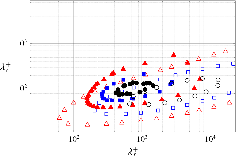
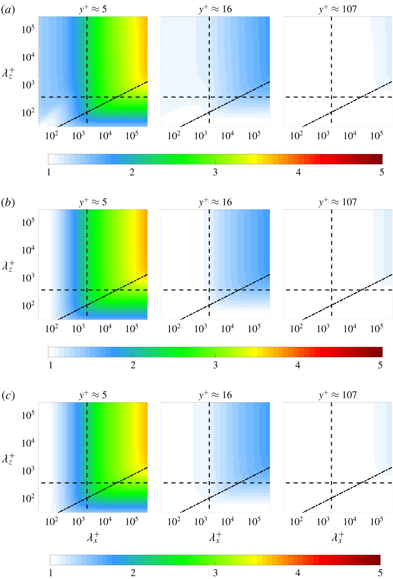
Premultiplied two-dimensional spectral density of streamwise velocity fluctuations $k_{x}k_{z}\int \unicode[STIX]{x1D6F7}_{\hat{u} ^{\prime }}(y;k_{x},k_{z},c)\,\text{d}c$ at $y^{+}\approx 5$ for Reynolds number $Re_{\unicode[STIX]{x1D70F}}=1000$. Contours are shown for 0.2 (▵, red), 0.5 (▫, blue), 0.8 (○, black) times the maximum value computed using the present approach. Results are plotted with the premultiplied spectral density of streamwise velocity fluctuations computed from DNS data. Contours are plotted at 0.2 (▴, red), 0.5 (▪, blue), 0.8 (●, black) times the maximum value from DNS data at $Re_{\unicode[STIX]{x1D70F}}=934$ (del Álamo et al. Reference del Álamo, Jiménez, Zandonade and Moser2004) (https://torroja.dmt.upm.es/channels/data/spectra/).

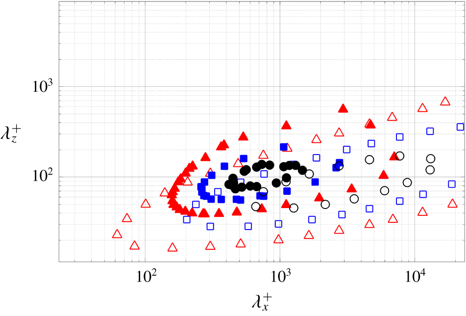
The averaging domain $\unicode[STIX]{x1D6FA}:(\unicode[STIX]{x1D706}_{x}^{+},\unicode[STIX]{x1D706}_{z}^{+})>(500,80)$ was chosen to include the sublayer streaks proposed as the source of the elevated near-wall convective velocity (Kim & Hussain Reference Kim and Hussain1993) but to avoid the nonlinear effects that dominate at smaller scales, where our linear analysis is not expected to be valid. The limitations of our input–output based approach at these smaller scales can be understood by examining the energy spectrum, which is compared to that of DNS data in figure 2. Here it is clear that the spectrum for DNS falls off much faster with decreasing wavelength than the spectrum obtained using the input–output based approach in this work. The relatively heavier weighting at the small scales (wavelength) structures imposed through the present approach results in a lower overall convective velocity in these regions. Our choice of averaging domain eliminates the effect of this heavier weighting and implicitly assumes that smaller wavelengths are energetically negligible. Therefore, these small wavelength components do not contribute to the average convective velocity computed using our input–output approach.

The performance of the input–output based model at small scales may be improved by integrating known correlations from DNS or experimental data; e.g. shaping the forcing based on spatial or temporal correlations obtained via simulation data (Moarref et al. Reference Moarref, Jovanović, Tropp, Sharma and McKeon2014; Zare et al. Reference Zare, Jovanović and Georgiou2017). Improvements could also potentially be realized by using an eddy viscosity based enhancement of the LNS equations (Reynolds & Hussain Reference Reynolds and Hussain1972), which Zare et al. (Reference Zare, Jovanović and Georgiou2017) have shown can provide similar improvements to the input–output response as the introduction of coloured-in-time forcing. Understanding the relative benefits of each of these approaches over the current model is a topic of ongoing work.

Figure 3.

(a) The average convective velocity of velocity fluctuations, $[\unicode[STIX]{x1D713}_{c}]_{h}^{+}(y)$: $\unicode[STIX]{x1D713}^{\prime }=u^{\prime }$ (▵, red), $\unicode[STIX]{x1D713}^{\prime }=v^{\prime }$ (▫, blue), $\unicode[STIX]{x1D713}^{\prime }=w^{\prime }$ (○, green) computed using the present approach and (5.1) with their corresponding weighting functions $h=\langle |{\mathcal{F}}_{xz}(\unicode[STIX]{x1D713}^{\prime })|^{2}\rangle k_{x}^{2}$ and an averaging domain of $(\unicode[STIX]{x1D706}_{x}^{+},\unicode[STIX]{x1D706}_{z}^{+})>(500,80)$ at $Re_{\unicode[STIX]{x1D70F}}=1000$. Results are plotted with convective velocities computed from DNS data (Geng et al. Reference Geng, He, Wang, Xu, Lozano-Durán and Wallace2015) at $Re_{\unicode[STIX]{x1D70F}}=932$: $\unicode[STIX]{x1D713}^{\prime }=u^{\prime }$ (——, red), $\unicode[STIX]{x1D713}^{\prime }=v^{\prime }$ (— ⋅ —, blue), $\unicode[STIX]{x1D713}^{\prime }=w^{\prime }$ (– –, green). (b) The model-based average convective velocity for streamwise fluctuations $\unicode[STIX]{x1D713}^{\prime }=u^{\prime }$ computed from (5.1) with the weighting function $h=\langle |{\mathcal{F}}_{xz}(u^{\prime })|^{2}\rangle k_{x}^{2}$ over averaging domain $(\unicode[STIX]{x1D706}_{x}^{+},\unicode[STIX]{x1D706}_{z}^{+})>(500,80)$ at $Re_{\unicode[STIX]{x1D70F}}=550$ ($\times$, red), $Re_{\unicode[STIX]{x1D70F}}=1000$ ($+$, blue), $Re_{\unicode[STIX]{x1D70F}}=5200$ (

, green). The black dashed lines in both (a) and (b) are the turbulent mean velocity profile at $Re_{\unicode[STIX]{x1D70F}}\approx 1000$ from Lee & Moser (Reference Lee and Moser2015).

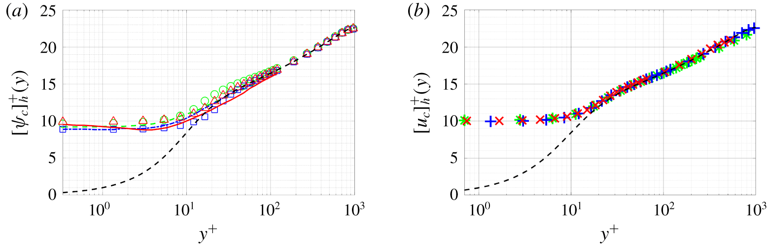
Figure 3(a) compares the resulting mean convective velocities to those obtained from the DNS data based computations of Geng et al. (Reference Geng, He, Wang, Xu, Lozano-Durán and Wallace2015). The plot demonstrates that the model-based average convective velocities of the streamwise, wall-normal and spanwise velocity fluctuations show good agreement with those computed from DNS data (Geng et al. Reference Geng, He, Wang, Xu, Lozano-Durán and Wallace2015).

Figure 3(b) replots the results for the streamwise velocity fluctuations in inner units for $Re_{\unicode[STIX]{x1D70F}}=550$, $Re_{\unicode[STIX]{x1D70F}}=1000$ and $Re_{\unicode[STIX]{x1D70F}}=5200$. The results collapse with the average convective velocities computed from the input–output based approach at different Reynolds numbers all tending to a constant value ${\approx}10u_{\unicode[STIX]{x1D70F}}$ near the wall. This Reynolds number invariance of convective velocities is consistent with the results reported in figure 3 of Geng et al. (Reference Geng, He, Wang, Xu, Lozano-Durán and Wallace2015).

The Reynolds number dependence can be analysed by rewriting (2.3a) and (2.3b) using the following change of variables $k_{x}=k_{x}^{+}Re_{\unicode[STIX]{x1D70F}}$, $\hat{\unicode[STIX]{x1D735}}=\hat{\unicode[STIX]{x1D735}}^{+}Re_{\unicode[STIX]{x1D70F}}$, $\text{d}\bar{u}/\text{d}y=Re_{\unicode[STIX]{x1D70F}}(\text{d}\bar{u}/\text{d}y^{+})$ and $\hat{\unicode[STIX]{x0394}}=\hat{\unicode[STIX]{x0394}}^{+}Re_{\unicode[STIX]{x1D70F}}^{2}$, which gives

(5.3a)$$\begin{eqnarray}\displaystyle & \displaystyle \text{i}k_{x}^{+}(\bar{u}-c)\hat{\boldsymbol{u}}^{\prime }-\hat{\unicode[STIX]{x0394}}^{+}\hat{\boldsymbol{u}}^{\prime }+\hat{v}^{\prime }\frac{\text{d}\bar{u}}{\text{d}y^{+}}\boldsymbol{i}+\hat{\unicode[STIX]{x1D735}}^{+}\hat{p}^{\prime }=\frac{\hat{\boldsymbol{f}}^{\prime }}{Re_{\unicode[STIX]{x1D70F}}}, & \displaystyle\end{eqnarray}$$

(5.3b)$$\begin{eqnarray}\displaystyle & \displaystyle \hat{\unicode[STIX]{x1D735}}^{+}\boldsymbol{\cdot }\hat{\boldsymbol{u}}^{\prime }=0. & \displaystyle\end{eqnarray}$$

As neither the mean velocity profile $\bar{u}$ nor the mean shear $\text{d}\bar{u}/\text{d}y^{+}$ at a specific $y^{+}$ vary over the Reynolds number in the near-wall region (see e.g. chap. 7.1.4 of Pope (Reference Pope2000)), the left-hand side of (5.3a) does not significantly vary over Reynolds number. The right-hand side of (5.3a) is related to $Re_{\unicode[STIX]{x1D70F}}$, but the Reynolds number only influences the magnitude of the stochastic forcing $\hat{\boldsymbol{f}}^{\prime }$. According to (3.6) and (3.7), the phase speed, $c$, at which $\unicode[STIX]{x1D6F7}_{\hat{u} ^{\prime }}$ peaks does not change, and thus, the convective velocity of the streamwise fluctuations, $u_{c}$ remains unaffected. This leads to the Reynolds number independence observed in figure 3(b).

This inner units scaling was also previously observed by Moarref et al. (Reference Moarref, Sharma, Tropp and McKeon2013) for streamwise energy density and further generalized by Sharma, Moarref & McKeon (Reference Sharma, Moarref and McKeon2017) in the framework of resolvent analysis. They end up with the same $Re_{\unicode[STIX]{x1D70F}}^{-1}$ scaling for the spatio-temporal transfer function as shown in (A4) of Moarref et al. (Reference Moarref, Sharma, Tropp and McKeon2013), and they also pointed out that $Re_{\unicode[STIX]{x1D70F}}$ independence of turbulent mean profile $\bar{u}(y)$ for $y^{+}\lesssim 100$ is necessary for this inner units scaling.

Having validated the ability of the input–output based computations to reproduce the mean trends, we next investigate the scale dependence of the convective velocity.

5.2 Scale-by-scale analysis of convective velocity

Figure 4.

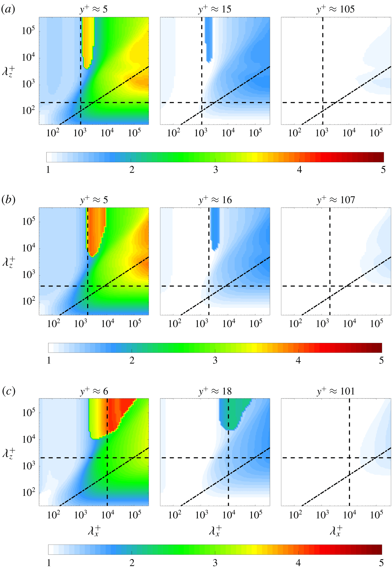
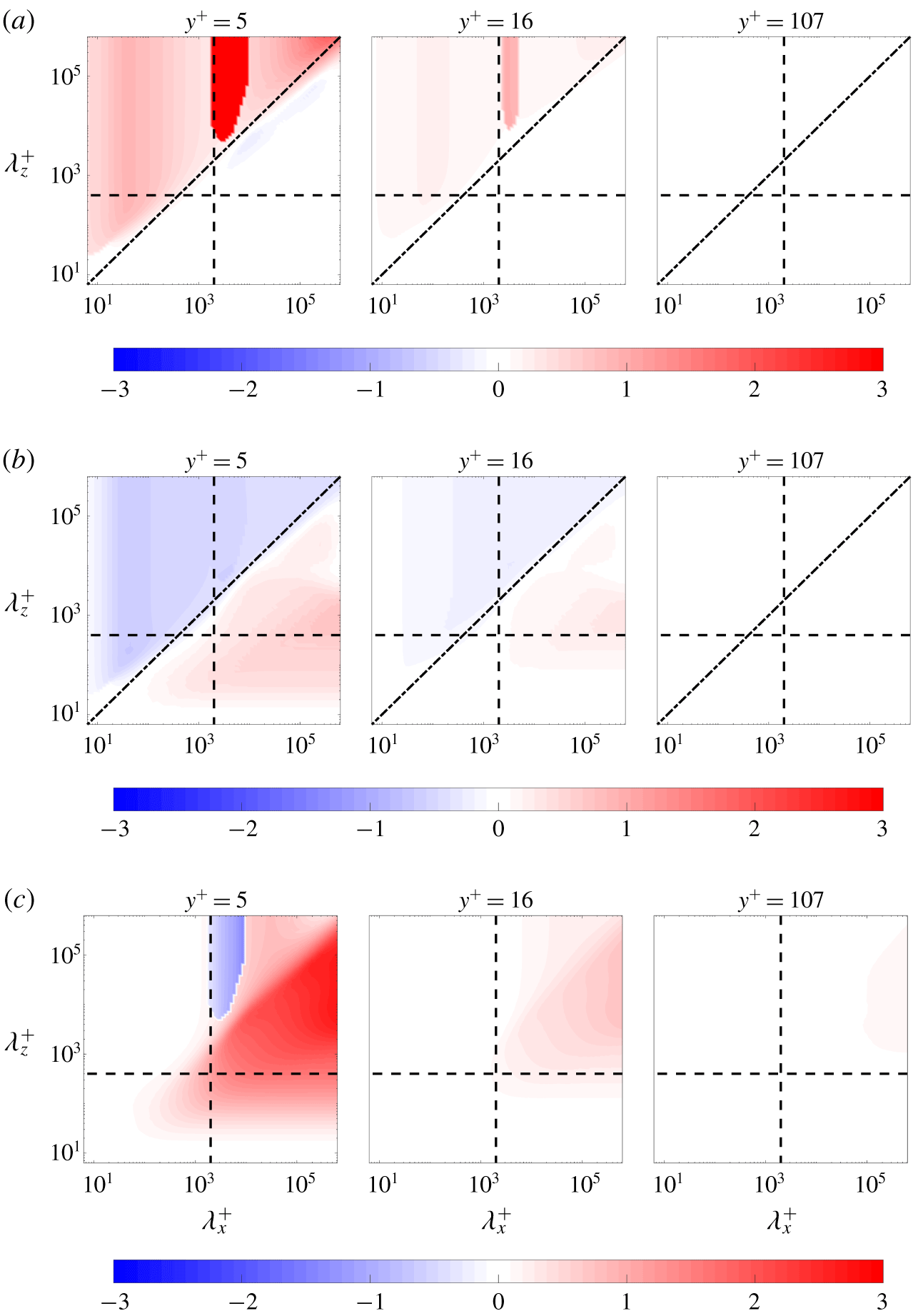
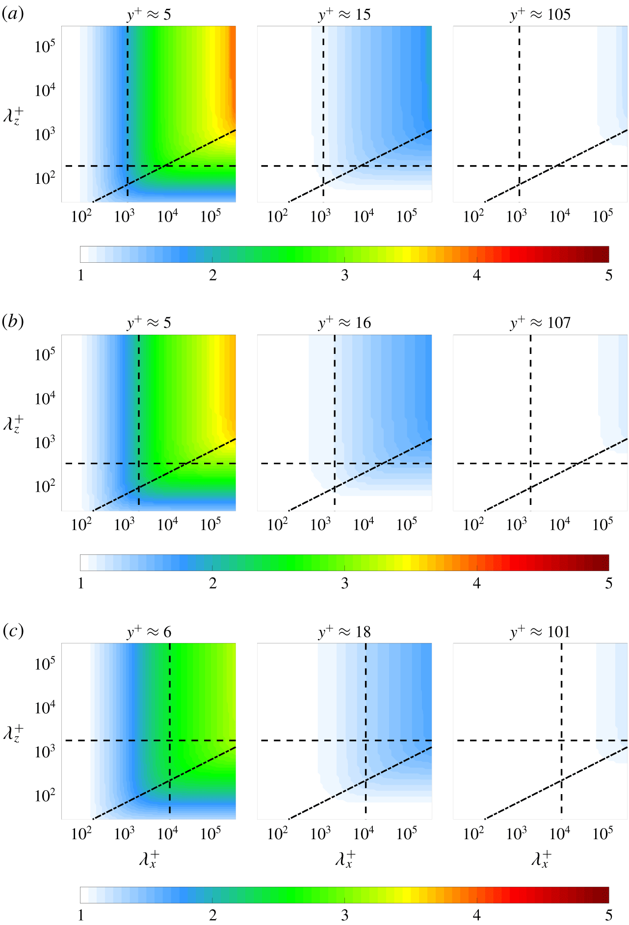
Scale-dependent convective velocity normalized by the local mean velocity $u_{c}(y;\unicode[STIX]{x1D706}_{x},\unicode[STIX]{x1D706}_{z})/\bar{u}(y)$ at (a) $Re_{\unicode[STIX]{x1D70F}}=550$, (b) $Re_{\unicode[STIX]{x1D70F}}=1000$ and (c) $Re_{\unicode[STIX]{x1D70F}}=5200$. The black dashed lines are given by $(\unicode[STIX]{x1D706}_{x},\unicode[STIX]{x1D706}_{z})=(2,0.4)$, which are identified by del Álamo & Jiménez (Reference del Álamo and Jiménez2009) as the lower bound of the large-scale convective velocity. The black dash-dot lines are $\unicode[STIX]{x1D706}_{z}^{+}={\unicode[STIX]{x1D706}_{x}^{+}}^{2/3}$, which fit through the knee of these contours.

The model-based approach employed herein allows one to calculate the contribution of each individual $(\unicode[STIX]{x1D706}_{x},\unicode[STIX]{x1D706}_{z})$ wavelength pair to the local convective velocity at each wall-normal location; i.e. $u_{c}(y;k_{x},k_{z})$. We now take advantage of this feature to investigate the scale-dependence of the convective velocity and examine which scales contribute to its deviation from the local mean velocity in various regions of the flow. Figure 4 shows the convective velocity of the streamwise velocity fluctuations normalized by the local mean velocity: $u_{c}(y;k_{x},k_{z})/\bar{u}(y)$ for (a) $Re_{\unicode[STIX]{x1D70F}}=550$, (b) $Re_{\unicode[STIX]{x1D70F}}=1000$ and (c) $Re_{\unicode[STIX]{x1D70F}}=5200$, as a function of the streamwise–spanwise wavelengths $(\unicode[STIX]{x1D706}_{x}^{+},\unicode[STIX]{x1D706}_{z}^{+})$ at wall-normal locations associated with the viscous sublayer ($y^{+}\approx 5$), the buffer layer ($y^{+}\approx 15$) and the log-law region ($y^{+}\approx 100$). As expected, the results in the viscous sublayer show the most significant deviations from the mean velocity, whereas there is little difference in the log-law region, which is consistent with the data in figure 3.

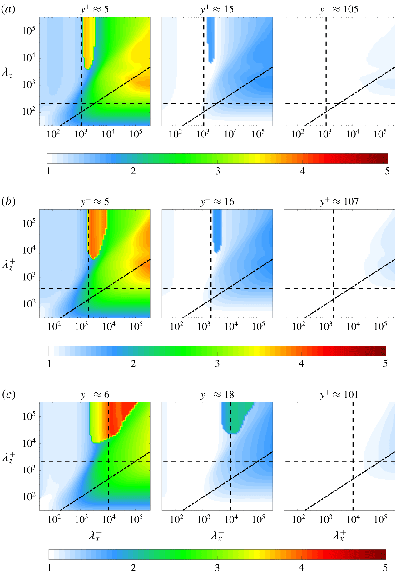
In figure 4, the convective velocities of structures in the intermediate scale range $\unicode[STIX]{x1D706}_{x}\approx 2$ show a discontinuity as the streamwise wavelength $\unicode[STIX]{x1D706}_{x}$ varies. This phenomenon was also observed for the scale-dependent convective velocity of wall pressure in pipe flow predicted using resolvent analysis with broadband forcing; see figure 12(a) in Luhar et al. (Reference Luhar, Sharma and McKeon2014). In the term-by-term analysis in § 7, we will further confirm that the convective velocity of structures associated with these scales is highly influenced by the pressure.

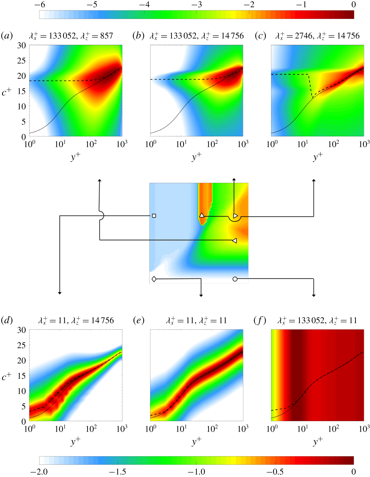
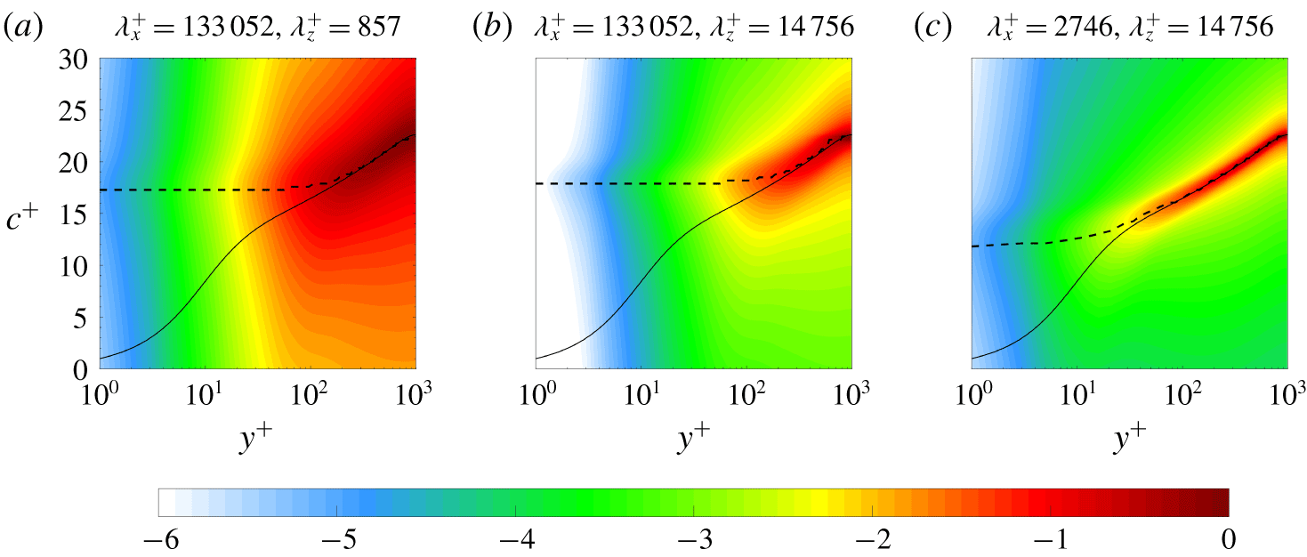
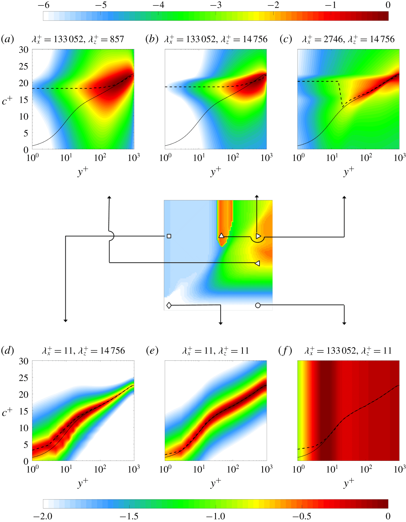
Figure 5 shows the PSD, $\unicode[STIX]{x1D6F7}_{\hat{u} ^{\prime }}(y;k_{x},k_{z},c)$ computed from (3.6), of the streamwise velocity fluctuations for $Re_{\unicode[STIX]{x1D70F}}=1000$ as a function of wall-normal location $y^{+}$ and phase speed $c^{+}$ at six different streamwise–spanwise wavelength pairs. Figures 5(a) and 5(b) show that the energy of the large wavelength structures at example points ◃ $(\unicode[STIX]{x1D706}_{x}^{+},\unicode[STIX]{x1D706}_{z}^{+})=(133\,052,857)$ and ▹ $(\unicode[STIX]{x1D706}_{x}^{+},\unicode[STIX]{x1D706}_{z}^{+})=(133\,052,14\,756)$, are concentrated near $(y^{+},c^{+})\approx (200,18.4)$, and that structures travelling at $c^{+}\approx 18.4$ provide the largest contribution to the spectral density in the near-wall region. Figure 5(c) indicates that structures travelling at a higher velocity than the local mean also contribute most to the PSD in the near-wall region for the intermediate-scale structures. In contrast, the PSD distributions over ($c^{+},y^{+}$) for structures with small streamwise wavelengths are more concentrated near the mean velocity profile $\bar{u}$ as shown in figures 5(d) and 5(e) for example points ▫ $(\unicode[STIX]{x1D706}_{x}^{+},\unicode[STIX]{x1D706}_{z}^{+})=(11,14\,756)$ and ♢ $(\unicode[STIX]{x1D706}_{x}^{+},\unicode[STIX]{x1D706}_{z}^{+})=(11,11)$.

Figure 5 indicates that the PSD distribution over phase speed is nearly symmetric about its peak in figures 5(a), 5(b), 5(d) and 5(e), which indicates close correspondence between the centre of gravity and peak of the PSD definitions of convective velocity. For the representative intermediate flow scale plotted in figure 5(c), the PSD distribution over the phase speed shows skewness, which is expected to lead to differences in the convective velocity obtained by considering the distribution. In order to evaluate the differences, we recomputed the results in figure 4(b) using a centre of gravity definition $\check{\unicode[STIX]{x1D713}}_{c}(y;k_{x},k_{z})\equiv (\int \!c\unicode[STIX]{x1D6F7}_{\hat{\unicode[STIX]{x1D713}}^{\prime }}(y;k_{x},k_{z},c)\,\text{d}c)/(\int \!\unicode[STIX]{x1D6F7}_{\hat{\unicode[STIX]{x1D713}}^{\prime }}(y;k_{x},k_{z},c)\,\text{d}c)$ and found that there are indeed differences for these scales. Specifically, the discontinuity in the convective velocity as streamwise wavelength $\unicode[STIX]{x1D706}_{x}$ varies over larger $\unicode[STIX]{x1D706}_{z}$ is smoothed. Differences also occur at the flow scales that are very small in the spanwise direction but very long in the streamwise direction; e.g. the structures indicated by ○ $(\unicode[STIX]{x1D706}_{x}^{+},\unicode[STIX]{x1D706}_{z}^{+})=(133\,052,11)$ in figure 5(f). These differences are not surprising because figure 5(f) demonstrates that the PSD is quite flat and therefore advection does not dominate at these flow scales. Here, neither definition of convective velocity is physically meaningful, as the maximum is not associated with a clear peak and the centre of gravity definition merely selects the centre point of the computational domain. The comparison verified that the overall trends that are highlighted in this manuscript, such as the influence of the large-scale structures in the near-wall and buffer regions as well as the slope of the knee through the contours indicated by dash-dot lines in the panels of figure 4 were unchanged when we used the centre of gravity in our computations. We therefore proceed with the definition in terms of the peak of the PSD in (3.7) in the remainder of the manuscript.

Figure 5.

Normalized power spectral density of streamwise velocity fluctuations $(\unicode[STIX]{x1D6F7}_{\hat{u} ^{\prime }}(y;k_{x},k_{z},c))/(\max _{c,y}(\unicode[STIX]{x1D6F7}_{\hat{u} ^{\prime }}(y;k_{x},k_{z},c)))$ over wall-normal location $y^{+}$ and phase speed $c^{+}$. The symbols represent locations associated with large-scale structures at (a) ◃ $(\unicode[STIX]{x1D706}_{x}^{+},\unicode[STIX]{x1D706}_{z}^{+})=(133\,052,857)$ and (b) ◃ $(\unicode[STIX]{x1D706}_{x}^{+},\unicode[STIX]{x1D706}_{z}^{+})=(133\,052,14\,756)$, (c) intermediate-scale structures ▵ $(\unicode[STIX]{x1D706}_{x}^{+},\unicode[STIX]{x1D706}_{z}^{+})=(2746,14\,756)$ and structures with small streamwise or spanwise wavelengths, respectively, (d) ▫ $(\unicode[STIX]{x1D706}_{x}^{+},\unicode[STIX]{x1D706}_{z}^{+})=(11,14\,756)$, (e) ♢ $(\unicode[STIX]{x1D706}_{x}^{+},\unicode[STIX]{x1D706}_{z}^{+})=(11,11)$ and (f) ○ $(\unicode[STIX]{x1D706}_{x}^{+},\unicode[STIX]{x1D706}_{z}^{+})=(133\,052,11)$. The colour is in base 10 logarithmic scale. The black solid lines represent the mean streamwise velocity profile and the black dashed lines are convective velocities computed using the method in § 3. The middle panel, which is reproduced from figure 4(b) at $y^{+}\approx 5$ for $Re_{\unicode[STIX]{x1D70F}}=1000$, indicates the locations corresponding to each symbol.

Both figures 4 and 5 indicate that large channel spanning structures have an influence on the convective velocity in both the viscous sublayer and the buffer layer. This phenomenon was investigated by del Álamo & Jiménez (Reference del Álamo and Jiménez2009), who identified large scales as structures of size $(\unicode[STIX]{x1D706}_{x},\unicode[STIX]{x1D706}_{z})>(2,0.4)$. This large-scale cut-off is identified by horizontal and vertical dashed lines in each panel of figure 4.

Figure 6.

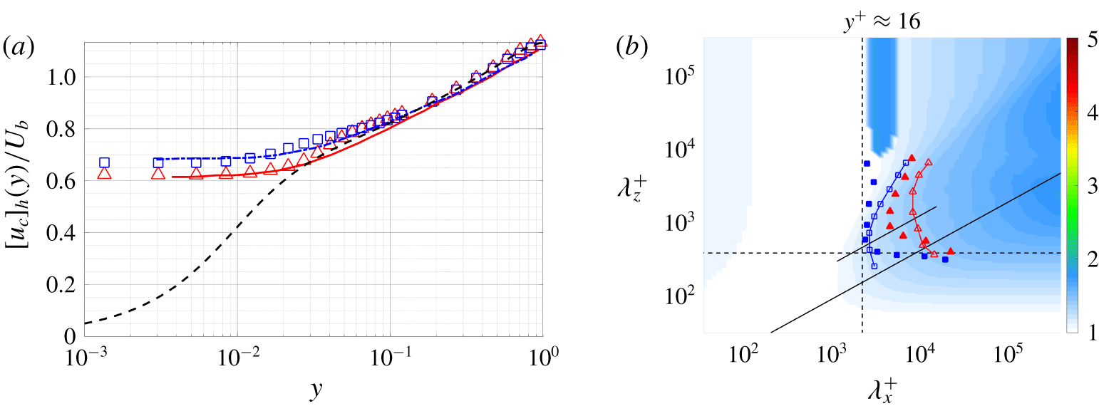
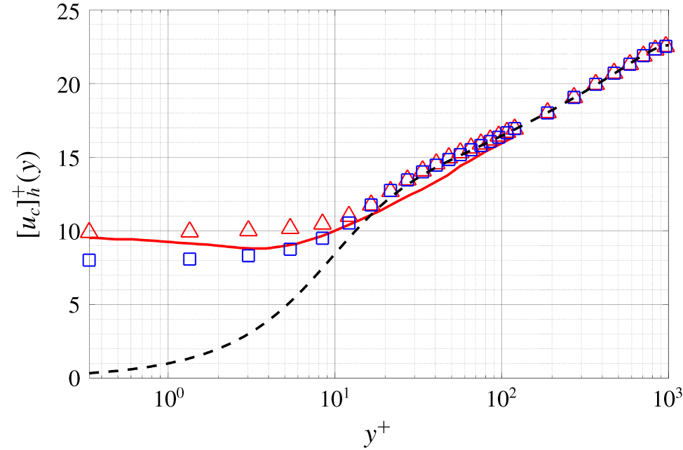
(a) The average convective velocity of streamwise fluctuations $[u_{c}]_{h}/U_{b}$ over $(\unicode[STIX]{x1D706}_{x},\unicode[STIX]{x1D706}_{z})>(2,0.4)$. Model based results at $Re_{\unicode[STIX]{x1D70F}}=550$ (▵, red) and $Re_{\unicode[STIX]{x1D70F}}=1000$ (▫, blue) are compared to convective velocities computed from DNS data (del Álamo & Jiménez Reference del Álamo and Jiménez2009) at $Re_{\unicode[STIX]{x1D70F}}=547$ (——, red) and $Re_{\unicode[STIX]{x1D70F}}=934$ (— ⋅ —, blue). For direct comparison with del Álamo & Jiménez (Reference del Álamo and Jiménez2009), the results in (a) are scaled by the bulk velocity; i.e. 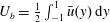$U_{b}=\frac{1}{2}\int _{-1}^{1}\bar{u}(y)\,\text{d}y$. The black dashed line is the mean velocity profile at $Re_{\unicode[STIX]{x1D70F}}\approx 1000$ from Lee & Moser (Reference Lee and Moser2015). (b) Model based scale-dependent convective velocity at $y^{+}\approx 16$ for $Re_{\unicode[STIX]{x1D70F}}=1000$: contour lines $u_{c}(y;k_{x},k_{z})/\bar{u}(y)=1.40$ (–▵–, red), $u_{c}(y;k_{x},k_{z})/\bar{u}(y)=1.21$ (–▫–, blue), are compared to convective velocities computed from DNS data at $y^{+}=15$ and $Re_{\unicode[STIX]{x1D70F}}=934$ (del Álamo & Jiménez Reference del Álamo and Jiménez2009) $u_{c}(y;k_{x},k_{z})/\bar{u}(y)=1.40$ (▴, red), $u_{c}(y;k_{x},k_{z})/\bar{u}(y)=1.21$ (▪, blue). The black dashed lines are given by $(\unicode[STIX]{x1D706}_{x},\unicode[STIX]{x1D706}_{z})=(2,0.4)$. The black solid lines are $\unicode[STIX]{x1D706}_{z}^{+}\sim {\unicode[STIX]{x1D706}_{x}^{+}}^{2/3}$, which fit through the knee of model based convective velocity and DNS data contours (del Álamo & Jiménez Reference del Álamo and Jiménez2009), respectively.

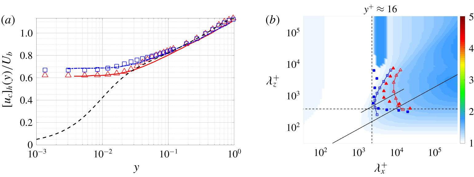
Figure 6(a) plots the mean convective velocities obtained for the averaging domain $(\unicode[STIX]{x1D706}_{x},\unicode[STIX]{x1D706}_{z})>(2,0.4)$ for $Re_{\unicode[STIX]{x1D70F}}=550$ and $Re_{\unicode[STIX]{x1D70F}}=1000$. A comparison with DNS data indicates that the model produces qualitatively and quantitatively similar behaviour to results computed from DNS data (figure 5a in del Álamo & Jiménez (Reference del Álamo and Jiménez2009)). Note the results in figure 6(a) are scaled by the bulk velocity; i.e. 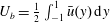$U_{b}=\frac{1}{2}\int _{-1}^{1}\bar{u}(y)\,\text{d}y$ for direct comparison with del Álamo & Jiménez (Reference del Álamo and Jiménez2009).

In figure 6(b), we further analyse the influence of the large scales by comparing the scale-dependent convective velocity at $y^{+}\approx 16$ with $Re_{\unicode[STIX]{x1D70F}}=1000$ from our approach to figure 3(a) in del Álamo & Jiménez (Reference del Álamo and Jiménez2009). The darker blue region of the largest $\unicode[STIX]{x1D706}_{x}^{+}$ and moderate-to-largest $\unicode[STIX]{x1D706}_{z}^{+}$ in figure 6(b) indicates the influence of large and very large-scale motion on the convective velocity in this region, which supports previous studies (Kim & Hussain Reference Kim and Hussain1993; Krogstad et al. Reference Krogstad, Kaspersen and Rimestad1998) indicating that fast moving structures centred further away from the wall (where the local mean velocity is larger) have an influence very near the wall due to their large size (Dinkelacker et al. Reference Dinkelacker, Hessel, Meier and Schewe1977; Kreplin & Eckelmann Reference Kreplin and Eckelmann1979; Farabee & Casarella Reference Farabee and Casarella1991; Kim & Hussain Reference Kim and Hussain1993; Hutchins et al. Reference Hutchins, Monty, Ganapathisubramani, Ng and Marusic2011).

A linear fit through the knee of the contour plot in figure 6(b) shows self-similar structures with a ratio $\unicode[STIX]{x1D706}_{z}^{+}\sim {\unicode[STIX]{x1D706}_{x}^{+}}^{2/3}$ in both our results and those reported in del Álamo & Jiménez (Reference del Álamo and Jiménez2009). This type of $x$–$z$ similarity in energy spectra density has been previously observed in the context of geometric self-similarity (del Álamo et al. Reference del Álamo, Jiménez, Zandonade and Moser2004; Chandran et al. Reference Chandran, Baidya, Monty and Marusic2017). For example, del Álamo and co-authors (del Álamo & Jiménez Reference del Álamo and Jiménez2003; del Álamo et al. Reference del Álamo, Jiménez, Zandonade and Moser2004) found that the isocontours of the premultiplied energy spectrum of $u^{\prime }$ form a corner centred along $\unicode[STIX]{x1D706}_{z}\sim \unicode[STIX]{x1D706}_{x}^{n}$ with $\frac{1}{3}<n<1$. In that work, the value of $n$ changed over the wall-normal location with lower bound on $n$ near the buffer layer ($y^{+}\approx 15$), increasing to $n=\frac{1}{2}$ in the log-law region and reaching $n=1$ in the outer region of the flow. Recent experimental measurements of two-dimensional spectra in zero-pressure gradient boundary layers indicate a $\unicode[STIX]{x1D706}_{z}\sim \sqrt{\unicode[STIX]{x1D706}_{x}}$ ($Re_{\unicode[STIX]{x1D70F}}=2430$) and $\unicode[STIX]{x1D706}_{z}\sim \unicode[STIX]{x1D706}_{x}$ ($Re_{\unicode[STIX]{x1D70F}}=26\,090$) relationship in the start of the log-law region (Chandran et al. Reference Chandran, Baidya, Monty and Marusic2016, Reference Chandran, Baidya, Monty and Marusic2017).

The scaling law of convective velocity explored here is closely related to the temporal self-similarity previously observed in the literature. More specifically, Lozano-Durán & Jiménez (Reference Lozano-Durán and Jiménez2014) showed that tall attached structures are both geometrically and temporally self-similar with lifetimes proportional to their distance from the wall. They also attribute the lifetime and deformation of these structures to the vertical gradient of their convective velocity. Long lifetimes, which require low dispersion, have been associated with coherent structures (Adrian Reference Adrian2007); e.g. hairpin vortices that are observed to propagate downstream with small velocity dispersion (Adrian, Meinhart & Tomkins Reference Adrian, Meinhart and Tomkins2000). Non-dispersive coherent structures are implied by the isocontour lines of the scale-dependent convective velocities in figures 4 and 6(b), which forms a $\unicode[STIX]{x1D706}_{z}^{+}\sim {\unicode[STIX]{x1D706}_{x}^{+}}^{2/3}$ knee. Based on this observation, we conjecture that the $x$–$z$ similarity observed here is closely related to the scaling laws of energy spectra.

To explain the $\unicode[STIX]{x1D706}_{z}^{+}\sim (\unicode[STIX]{x1D706}_{x}^{+})^{2/3}$ scaling, we employ a simple model involving the bending of streamlines in the cross-plane due to the presence of a streamwise vortex. This simple model was originally proposed by Jiménez, del Álamo & Flores (Reference Jiménez, del Álamo and Flores2004) to explain the contribution of high-momentum streaks to the energy spectrum. Consider convection of $\hat{u} ^{\prime }$ due to a point vortex with circulation $\unicode[STIX]{x1D6FE}$ in the cross-plane $\unicode[STIX]{x2202}_{t}u^{\prime }+(2\unicode[STIX]{x03C0}\unicode[STIX]{x1D6FE}/r^{2})(\unicode[STIX]{x2202}u^{\prime }/\unicode[STIX]{x2202}\unicode[STIX]{x1D703})=0$ where $(r,\unicode[STIX]{x1D703})$ is the polar representation of the $(y,z)$ plane, centred on the vortex. For a homogeneous shear initial condition, $u^{\prime }(t=0,r,\unicode[STIX]{x1D703})\sim Sy=Sr\sin \unicode[STIX]{x1D703}$, with shear rate $S$, we have $u^{\prime }(t,r,\unicode[STIX]{x1D703})\sim Sr\sin (\unicode[STIX]{x1D703}-\unicode[STIX]{x1D6FE}t/2\unicode[STIX]{x03C0}r^{2})$. At a given time, $t$, setting $\unicode[STIX]{x1D703}=\unicode[STIX]{x03C0}$ yields the ‘size’ of the vortex-distorted region as

(5.4)$$\begin{eqnarray}R_{z}=\sqrt{\unicode[STIX]{x1D6FE}t/2\unicode[STIX]{x03C0}^{2}}.\end{eqnarray}$$

Moreover, the length of streak is determined by the velocity difference between its top and bottom with shear rate $S$, which can be roughly estimated as

(5.5)$$\begin{eqnarray}\unicode[STIX]{x1D706}_{x}=SR_{z}t,\end{eqnarray}$$

if we assume that the streak height is roughly equal to its width. We estimate the meandering magnitude of streaks by approximating the spanwise drift of the vortices under the induction of their reflected images across the wall, which leads to

(5.6)$$\begin{eqnarray}\unicode[STIX]{x1D706}_{z}=2\sqrt{2}w^{\prime }t,\end{eqnarray}$$

where $w^{\prime }$ denotes a spanwise velocity fluctuation of the order of ${w^{\prime }}^{+}\approx 1$ (Kim, Moin & Moser Reference Kim, Moin and Moser1987). Combining equations (5.4), (5.5) and (5.6) gives the scaling

(5.7)$$\begin{eqnarray}\unicode[STIX]{x1D706}_{z}^{+}\sim (\unicode[STIX]{x1D706}_{x}^{+})^{2/3}.\end{eqnarray}$$

Although this is an idealized analysis, it leads to the trends observed both here and in DNS-based convective velocity analysis. The assumptions underlying this scaling are also consistent with the existence of structures at a wide variety of scales extending into the channel; i.e. structures reminiscent of Townsend’s attached eddies (Townsend Reference Townsend1976; Perry, Henbest & Chong Reference Perry, Henbest and Chong1986; Marusic & Monty Reference Marusic and Monty2019). We next calculate the wall-normal coherence of these structures to further examine this connection.

Figure 7.

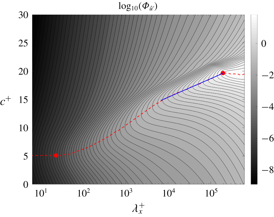
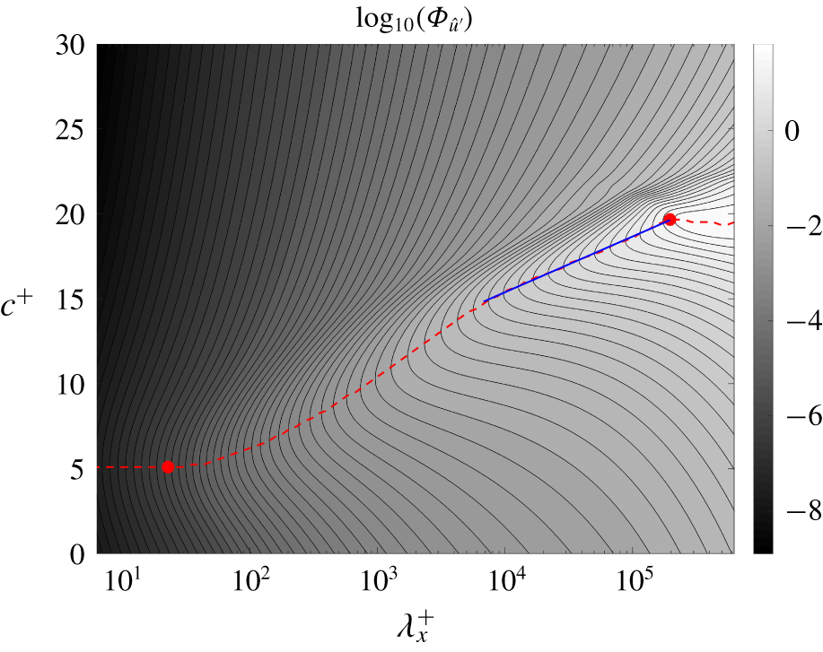
Isocontours of $\unicode[STIX]{x1D6F7}_{\hat{u} ^{\prime }}$ in the viscous sublayer ($y^{+}\approx 5$) along $\unicode[STIX]{x1D706}_{z}^{+}=(\unicode[STIX]{x1D706}_{x}^{+})^{2/3}$ at $Re_{\unicode[STIX]{x1D70F}}=1000$, calculated using (3.6). The red dashed line indicates the $c^{+}$ at which $\unicode[STIX]{x1D6F7}_{\hat{u} ^{\prime }}$ peaks for each $\unicode[STIX]{x1D706}_{x}^{+}$, and the blue solid line indicates the region of logarithmic increase. It therefore defines the convective velocity $u_{c}$ as in (3.7). The markers (●, red) indicate the locations where we evaluate the two-point wall-normal coherence in figure 8.

6 Wall-normal coherence of viscous sublayer structures

The convective velocity at each $(\unicode[STIX]{x1D706}_{x},\unicode[STIX]{x1D706}_{z})$ wavelength pair, $u_{c}(y;k_{x},k_{z})$, is obtained via the maximization in (3.7), so we refer to the spectral component of $u^{\prime }$ defined by $(\unicode[STIX]{x1D706}_{x},\unicode[STIX]{x1D706}_{z},u_{c})$ as the ‘characteristic structure’. We hypothesize that the characteristic structure at a given wall-normal location, $y_{0}$, is responsible for the dominant convection at that location, and that it also contributes to the energetics elsewhere in the channel due to its wall-normal extent. In this section, we investigate this wall-normal extent using the spectral coherence between signals at two different wall-normal locations. We focus on the characteristic structures that provide the dominant convection in the viscous sublayer and on wavelength pairs along the knee of the isocontours of $u_{c}$ in figure 4; i.e. along $\unicode[STIX]{x1D706}_{z}^{+}=(\unicode[STIX]{x1D706}_{x}^{+})^{2/3}$.

The $u^{\prime }$ frequency–wavenumber spectrum, $\unicode[STIX]{x1D6F7}_{\hat{u} ^{\prime }}=\langle |\hat{u} ^{\prime }|^{2}\rangle$ of streamwise fluctuations in the viscous sublayer ($y^{+}\approx 5$) for $Re_{\unicode[STIX]{x1D70F}}=1000$, is shown in figure 7 in terms of phase speed and wavelength along $\unicode[STIX]{x1D706}_{z}^{+}=(\unicode[STIX]{x1D706}_{x}^{+})^{2/3}$. The autocorrelation maxima defining the convective velocity are plotted as a dashed line. The ridge corresponding to these maximum values asymptote to constants at both the large and small wavelength limits, but show a region of linear growth followed by a region of logarithmic increase (blue solid line) between two red circle markers. The logarithmic behaviour is similar to the variation of the mean velocity profile $\bar{u}(y)$ with $y$ and is consistent with the assumption that the dominant viscous sublayer convection at streamwise wavelength $\unicode[STIX]{x1D706}_{x}$ arises due to a structure advecting at the local mean velocity at $y\sim \unicode[STIX]{x1D706}_{x}^{n}$ for some $n>0$.

Figure 8.

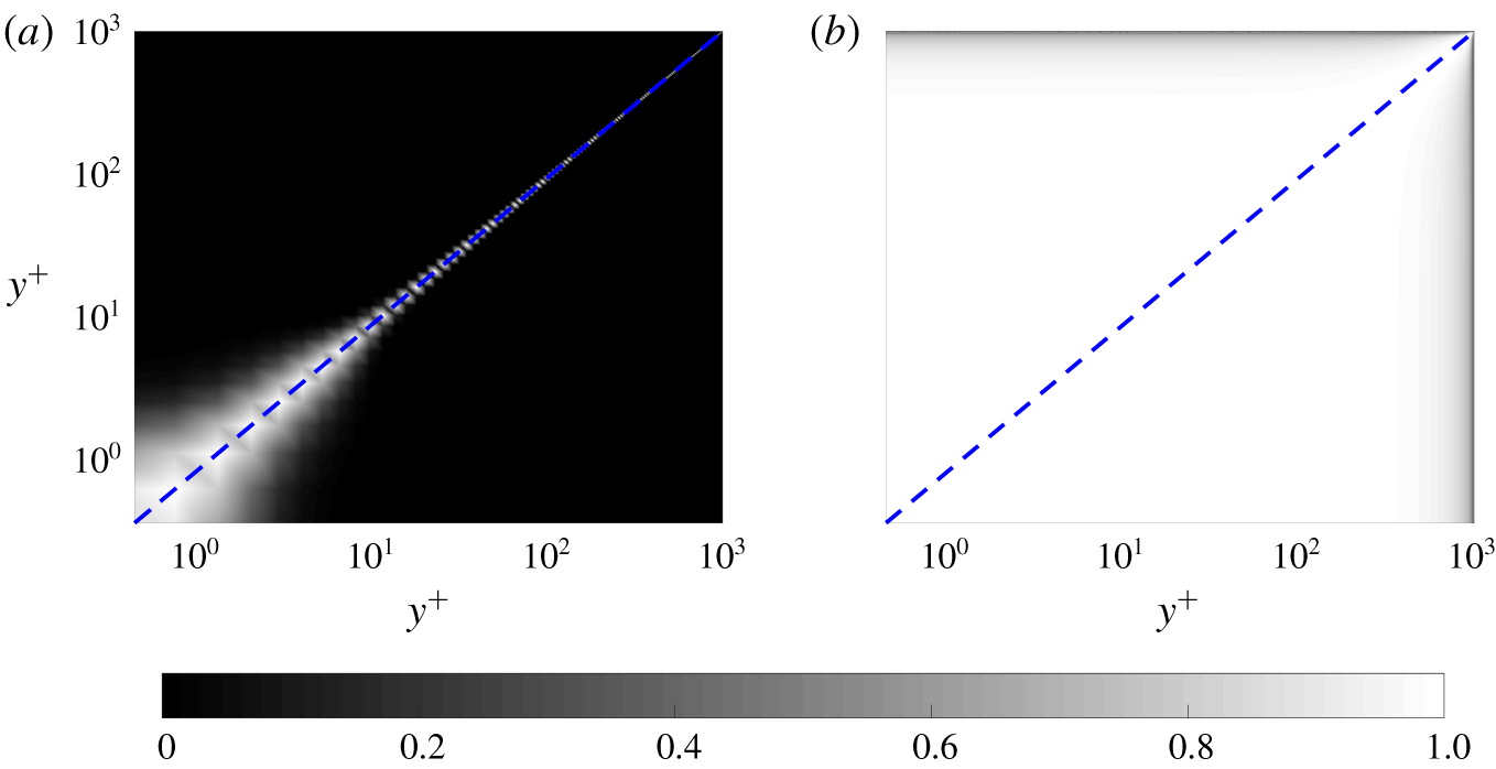
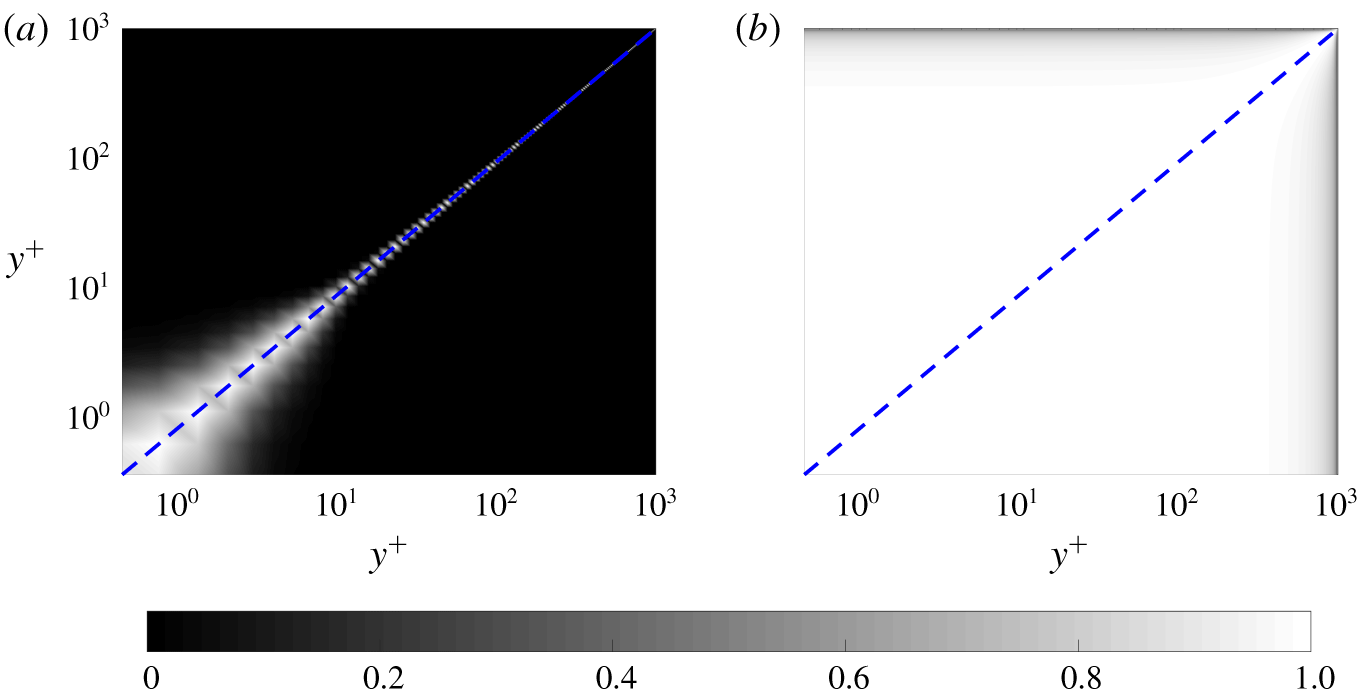
Two-point spectral coherence of streamwise velocity fluctuations $\unicode[STIX]{x1D712}_{u^{\prime };y^{\prime }y}$ for data at $Re_{\unicode[STIX]{x1D70F}}=1000$, as defined in (6.1) at (a) $(\unicode[STIX]{x1D706}_{x}^{+},\unicode[STIX]{x1D706}_{z}^{+})\approx (22,8)$ and (b) $(\unicode[STIX]{x1D706}_{x}^{+},\unicode[STIX]{x1D706}_{z}^{+})\approx (2\times 10^{5},3\times 10^{3})$ indicated by circle markers in figure 7. Both points are along $\unicode[STIX]{x1D706}_{z}^{+}=(\unicode[STIX]{x1D706}_{x}^{+})^{2/3}$, and their phase speeds in friction units are approximately $c^{+}\approx 5$ for the small-scale structure and $c^{+}\approx 20$ for the large one. Perfectly coherent signals have a spectral coherence of $1$, and incoherent signals have a spectral coherence of $0$.

The spectral coherence between two wall-normal locations $y^{\prime }$ and $y$, defined for a fluctuating variable $\unicode[STIX]{x1D713}$ is defined as

(6.1)$$\begin{eqnarray}0\leqslant \unicode[STIX]{x1D712}_{\unicode[STIX]{x1D713}^{\prime };y^{\prime }y}(k_{x},k_{z},c)\equiv \frac{|\unicode[STIX]{x1D6F7}_{\hat{\unicode[STIX]{x1D713}}^{\prime },cross}(y^{\prime },y;k_{x},k_{z},c)|^{2}}{\unicode[STIX]{x1D6F7}_{\hat{\unicode[STIX]{x1D713}}^{\prime }}(y^{\prime };k_{x},k_{z},c)\unicode[STIX]{x1D6F7}_{\hat{\unicode[STIX]{x1D713}}^{\prime }}(y;k_{x},k_{z},c)}\leqslant 1,\end{eqnarray}$$

where $\unicode[STIX]{x1D6F7}_{\hat{\unicode[STIX]{x1D713}}^{\prime },cross}$ is the cross-spectral density of $\unicode[STIX]{x1D713}^{\prime }$ between locations $y^{\prime }$ and $y$; i.e.

(6.2)$$\begin{eqnarray}\unicode[STIX]{x1D6F7}_{\hat{\unicode[STIX]{x1D713}}^{\prime },cross}(y^{\prime },y;k_{x},k_{z},c)=\langle \hat{\unicode[STIX]{x1D713}}^{\prime \ast }(y^{\prime };k_{x},k_{z},c)\hat{\unicode[STIX]{x1D713}}^{\prime }(y;k_{x},k_{z},c)\rangle .\end{eqnarray}$$

The cross-spectral densities are the off-diagonal components of the matrix obtained from the finite-dimensional representation (4.1) of $\unicode[STIX]{x1D6F7}_{\hat{\unicode[STIX]{x1D713}}^{\prime }}$. Figure 8 shows the two-point spectral coherence for streamwise velocity fluctuations $\unicode[STIX]{x1D712}_{u^{\prime };y^{\prime }y}$ for two characteristic structures along $\unicode[STIX]{x1D706}_{z}^{+}=(\unicode[STIX]{x1D706}_{x}^{+})^{2/3}$ in the near-wall region: (a) a short wavelength component, $(\unicode[STIX]{x1D706}_{x}^{+},\unicode[STIX]{x1D706}_{z}^{+})\approx (22,8)$, and (b) a long wavelength component, $(\unicode[STIX]{x1D706}_{x}^{+},\unicode[STIX]{x1D706}_{z}^{+})\approx (2\times 10^{5},3\times 10^{3})$. The phase speeds associated with these characteristic structures are indicated in figure 7 by circle markers. The shorter wavelength component is associated with the smaller convective velocity and the longer wavelength component with the larger convective velocity.

In figure 8, we see a wall-normal coherence that extends from the wall; i.e. it does not involve any wall-detached patches, consistent with Townsend’s attached-eddy hypothesis (Townsend Reference Townsend1976; Perry et al. Reference Perry, Henbest and Chong1986; Marusic & Monty Reference Marusic and Monty2019). As predicted by del Álamo & Jiménez (Reference del Álamo and Jiménez2009), the long wavelength component is more coherent further into the channel towards the core than the short wavelength component with its coherence falling to zero in the core. This growth of coherence away from the wall with increasing wavelength suggests that the structures contributing to the convective velocity in the viscous sublayer extend from the wall deep into the log-law region, but only weakly into the wake region, reminiscent of the long meandering structures in the log-law region whose footprint extends to the near-wall region (Jiménez et al. Reference Jiménez, del Álamo and Flores2004; Guala et al. Reference Guala, Hommema and Adrian2006; Balakumar & Adrian Reference Balakumar and Adrian2007; Hutchins & Marusic Reference Hutchins and Marusic2007; Monty et al. Reference Monty, Stewart, Williams and Chong2007).

Calculations (not presented here for brevity) indicate that components with identical convective velocity as determined by figure 4 also have nearly identical wall-normal coherence. This behaviour, also suggested by del Álamo & Jiménez (Reference del Álamo and Jiménez2009), agrees with the hypothesis that a random arrangement of similar basic structures with dimensions given by $\unicode[STIX]{x1D706}_{z}^{+}=(\unicode[STIX]{x1D706}_{x}^{+})^{2/3}$, leads to the long-tailed behaviour of the contours in figure 4.

Figure 9.

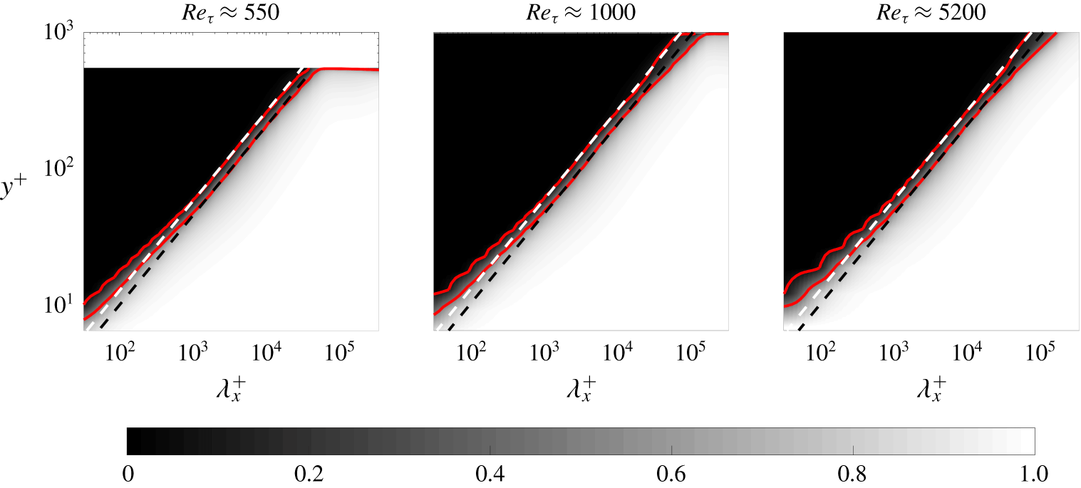
Two-point spectral coherence of streamwise velocity fluctuations $\unicode[STIX]{x1D712}_{u^{\prime };y^{\prime }y}$ at $Re_{\unicode[STIX]{x1D70F}}\approx 550$, $Re_{\unicode[STIX]{x1D70F}}\approx 1000$ and $Re_{\unicode[STIX]{x1D70F}}\approx 5200$, as defined in (6.1), between ${y^{\prime }}^{+}\approx y_{sublayer}^{+}=5$ and wall-normal locations above it for wavelengths defined by $\unicode[STIX]{x1D706}_{z}^{+}=(\unicode[STIX]{x1D706}_{x}^{+})^{2/3}$ and phase speeds indicated by the dashed maxima line in figure 7. The solid red lines serve to indicate the boundaries of regions of high/low coherence and are isocontours of spectral coherence with values 0.1 and 0.5. The white dashed lines are $y^{+}=0.55(\unicode[STIX]{x1D706}_{x}^{+})^{2/3}$ and the black dashed lines are $y^{+}=0.43(\unicode[STIX]{x1D706}_{x}^{+})^{2/3}$ and they serve as fits to the red lines. Perfectly coherent signals have a spectral coherence of $1$, and incoherent signals have a spectral coherence of $0$.

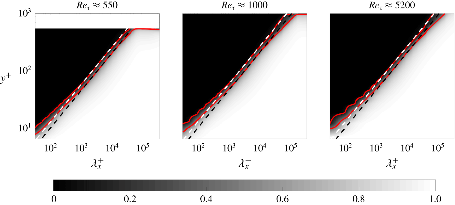
Figure 9 shows the spectral coherence with respect to the viscous sublayer location ($y_{sublayer}^{+}\equiv 5$) $\unicode[STIX]{x1D712}_{u^{\prime };y_{sublayer}y}(k_{x},k_{z},c)$ along $\unicode[STIX]{x1D706}_{z}^{+}=(\unicode[STIX]{x1D706}_{x}^{+})^{2/3}$. The monotonic behaviour of the spectral coherence in figure 9 implies that structures larger in $(x,z)$ are also larger in $y$. The wall-normal coherence for $\unicode[STIX]{x1D706}_{x}^{+}\gtrsim 200$ indicated by the dashed lines overlain on the (red) solid contours representing spectral coherences of $0.1$ and $0.5$ shows an aspect ratio $y^{+}\sim (\unicode[STIX]{x1D706}_{x}^{+})^{2/3}$. The minimum wall-normal coherence length associated with these larger wavelengths is ${\sim}15$ wall units, which is the approximate location of the buffer layer and also the location of the well-known peak in the root-mean-square streamwise velocity fluctuations; see for example, Lee & Moser (Reference Lee and Moser2015). This self-similarity represented by a power-law relationship at larger wavelengths is also suggestive of the attached-eddy structures proposed by Townsend (Reference Townsend1976), Perry et al. (Reference Perry, Henbest and Chong1986) and Marusic & Monty (Reference Marusic and Monty2019).

From the power-law behaviour $y^{+}\sim (\unicode[STIX]{x1D706}_{x}^{+})^{2/3}$ for $\unicode[STIX]{x1D706}_{x}^{+}\gtrsim 200$ shown in figure 9, we can also extract the structure inclination angle contributing to this self-similar behaviour. The $0.1$ and $0.5$ spectral coherence contour is fitted by $y^{+}=\unicode[STIX]{x1D6FC}(\unicode[STIX]{x1D706}_{x}^{+})^{2/3}$ with $\unicode[STIX]{x1D6FC}=0.55$ (white dash lines) and $\unicode[STIX]{x1D6FC}=0.43$ (black dash lines), respectively. We select the spectral coherence contours as 0.1 and 0.5 to fit the scaling laws because we observe significant variation of coherence between this range in figure 9, while outside of this range, the coherence shows saturation. Such a saturation phenomenon is also observed in the coherence computed from the experimental data; see e.g. figure 4 of Baars, Hutchins & Marusic (Reference Baars, Hutchins and Marusic2016) and figure 5(b) of Baars, Hutchins & Marusic (Reference Baars, Hutchins and Marusic2017). Furthermore, the contours of two-dimensional spectral coherence of $0.1$, $0.3$ and $0.5$ are shown to collapse when scaled with the wall-normal height of the structures; indicating the presence of self-similar structures; see figure 4 of Madhusudanan et al. (Reference Madhusudanan, Illingworth and Marusic2019).

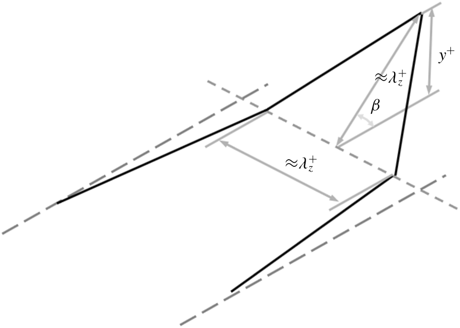
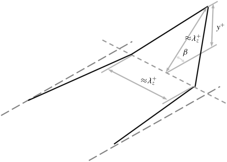
Thus, $y^{+}\sim \unicode[STIX]{x1D706}_{z}^{+}$ with a constant of proportionality $\unicode[STIX]{x1D6FC}$ between $0.55$ and $0.43$, respectively, implies that the projection of the structures onto the cross-stream plane has a smaller height than width. If we assume the structures contributing to the spectral coherence have a height/width aspect ratio of $1$, as depicted in the cartoon in figure 10, then the dimensions of the cross-plane projection of the structure represented by spectral coherence between $0.1$ and $0.5$ implies a tilt angle $\unicode[STIX]{x1D6FD}=\text{arcsin}(\unicode[STIX]{x1D6FC})$ between approximately $25^{\circ }$ and $33^{\circ }$.

Figure 10.

The structures of height/width aspect ratio 1 with an inclination angle $\unicode[STIX]{x1D6FD}$ in analogy with Perry & Chong (Reference Perry and Chong1982).

Townsend (Reference Townsend1976) suggests an inclination angle of ${\sim}30^{\circ }$ for attached double roller eddies (a pair of counter-rotating, inclined, approximately streamwise vortex structures) to explain the experimental observations of Grant (Reference Grant1958). Experimental observations in turbulent boundary layers, on the other hand, have yielded inclination angles between $15^{\circ }$ and $20^{\circ }$ (Brown & Thomas Reference Brown and Thomas1977; Carper & Porté-Agel Reference Carper and Porté-Agel2004; Marusic & Heuer Reference Marusic and Heuer2007). The latter inclination angles were calculated using two-point temporal correlations and Taylor’s hypothesis. In turbulent channel flows, hairpin vortices have been the focus of considerable interest. Although a single well-defined inclination angle cannot be associated with hairpin vortices, the inclinations of hairpin-like structures vary from $12^{\circ }$ (elongated legs) to $45^{\circ }$ (hairpin heads) (Adrian Reference Adrian2007). The present work does not restrict the structures contributing to the convective velocities to any one of the structures discussed above, but does provide an inclination angle, assuming structures are roughly of aspect ratio $1$, which is within the range of previous observations.

In figure 9, the structure inclination angle predicted by this model also shows Reynolds number invariance, which is consistent with experimental observations (Marusic & Heuer Reference Marusic and Heuer2007). For different Reynolds numbers, $y^{+}=\unicode[STIX]{x1D6FC}(\unicode[STIX]{x1D706}_{x}^{+})^{2/3}$ with $\unicode[STIX]{x1D6FC}=0.55$ and $\unicode[STIX]{x1D6FC}=0.43$, corresponding to tilt angles $25^{\circ }$ and $33^{\circ }$, always give good approximations for $0.1$ and $0.5$ spectral coherence, respectively. Structure inclination angles inferred from the cross correlation of $x$ in the experimental studies of Marusic & Heuer (Reference Marusic and Heuer2007) are found to be invariant over three orders of magnitude change in Reynolds number.

Our results reveal that the contributions from the relatively larger scale structures lead to the elevated velocities in the viscous sublayer seen in figure 3 and that these structures have dimensions given by $y^{+}\sim \unicode[STIX]{x1D706}_{z}^{+}\sim (\unicode[STIX]{x1D706}_{x}^{+})^{2/3}$ with a minimum size ${\approx}15$ friction units, which is the approximate location of the buffer layer. The inclination angles of these structures do not vary with Reynolds number, which is consistent with experimental observations. These observations are consistent with the attached-eddy hypothesis in that they predict wall-attached structures that are self-similar in the cross-plane and contribute to the dominant convection. However, the attached-eddy hypothesis predicts that these structures are also self-similar in the streamwise direction, which our approach does not show.

7 Term-by-term analysis of scale-dependent convective velocities

We next use the input–output framework to analyse the contribution of different linear mechanisms to the scale-dependent convective velocity of the streamwise velocity fluctuations.

We follow the method shown in (2.11) of del Álamo & Jiménez (Reference del Álamo and Jiménez2009) to obtain the normalized deviation of the convective velocity from the mean velocity contributed from various terms. In particular, we multiply the $x$-momentum in (2.3a) by $\hat{u} ^{\prime \ast }$ and take the imaginary part of the result to obtain

(7.1)$$\begin{eqnarray}\frac{u_{c}-\bar{u}(y)}{\bar{u}(y)}=\frac{\displaystyle \overbrace{k_{x}\text{Re}\{\langle \hat{p}^{\prime }\hat{u} ^{\prime \ast }\rangle \}}^{\text{IIa}}+\text{Im}\left\{\overbrace{\frac{\text{d}\bar{u}}{\text{d}y}\langle \hat{v}^{\prime }\hat{u} ^{\prime \ast }\rangle }^{\text{IIb}}\overbrace{-\frac{1}{Re_{\unicode[STIX]{x1D70F}}}\langle \hat{u} ^{\prime \ast }\unicode[STIX]{x2202}_{yy}^{2}\hat{u} ^{\prime }\rangle }^{\text{IIc}}\overbrace{-\langle \hat{f_{u}}^{\prime }\hat{u} ^{\prime \ast }\rangle }^{\text{III}}\right\}}{k_{x}\bar{u}(y)\langle \hat{u} ^{\prime }\hat{u} ^{\prime \ast }\rangle }.\end{eqnarray}$$

Here $\text{Re}\{\cdot \}$ and $\text{Im}\{\cdot \}$ represent the respective real part and imaginary part of the argument. The terms in (7.1) represent the relative contributions of the pressure term (IIa), the mean shear term (IIb), and the viscous term (IIc), each normalized by $k_{x}\bar{u}(y)\langle \hat{u} ^{\prime }\hat{u} ^{\prime \ast }\rangle$.

We compute each term in (7.1) by modifying the output operator in (3.4) and then computing the cross-spectra through an appropriate modification of (3.6). For example, we can use the output operator corresponding to the fluctuating pressure in (3.9) to obtain ${\mathcal{G}}_{\hat{p}^{\prime }}$ and then compute the cross-spectra as

(7.2)$$\begin{eqnarray}\langle \hat{p}^{\prime }\hat{u} ^{\prime \ast }\rangle ={\mathcal{G}}_{\hat{p}^{\prime }}\langle \hat{\boldsymbol{f}}^{\prime }\hat{\boldsymbol{f}}^{\prime \ast }\rangle {\mathcal{G}}_{\hat{u} ^{\prime }}^{\ast }={\mathcal{G}}_{\hat{p}^{\prime }}{\mathcal{G}}_{\hat{u} ^{\prime }}^{\ast }.\end{eqnarray}$$

The other terms in (7.1) can be computed in a similar manner.

Figure 11.

Different linear terms’ contributions to scale-dependent convective velocities $(u_{c}(y;k_{x},k_{z})-\bar{u}(y))/\bar{u}(y)$ quantified using (7.1): (a) the pressure term (IIa), (b) the mean shear term (IIb) and (c) the viscous term (IIc). All terms are normalized by $k_{x}\bar{u}(y)\langle \hat{u} ^{\prime }\hat{u} ^{\prime \ast }\rangle$. The Reynolds number is $Re_{\unicode[STIX]{x1D70F}}=1000$. The black dashed lines are given by $(\unicode[STIX]{x1D706}_{x},\unicode[STIX]{x1D706}_{z})=(2,0.4)$, and the black dash-dot lines in (a) and (b) are $\unicode[STIX]{x1D706}_{z}^{+}=\unicode[STIX]{x1D706}_{x}^{+}$. Note that the white region of the colour map represents a value close to zero.

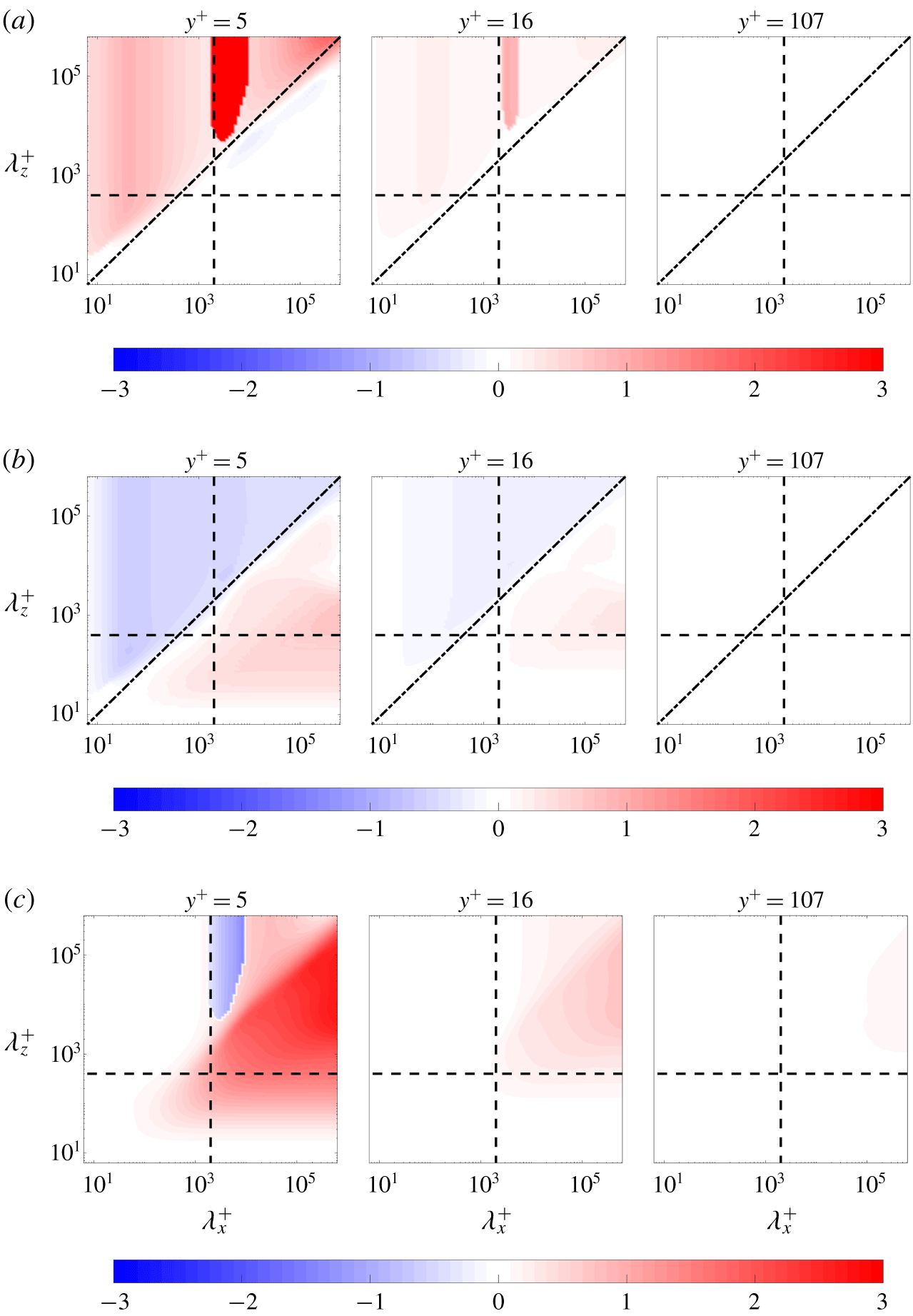
Figure 11(a–c) shows the respective contributions from the pressure term (IIa), the mean shear term (IIb) and the viscous term (IIc) to the scale-dependent convective velocity of the streamwise velocity fluctuations ($Re_{\unicode[STIX]{x1D70F}}\approx 1000$) at the same three wall-normal locations as in figure 4. As shown in figure 11(a), the pressure plays an important role for the intermediate scale structures ($\unicode[STIX]{x1D706}_{x}\approx 2$ and $\unicode[STIX]{x1D706}_{z}>\unicode[STIX]{x1D706}_{x}$), which supports our conjecture that the discontinuity in these scales shown in figure 4 is related to the pressure. Luhar et al.’s (Reference Luhar, Sharma and McKeon2014) figure 12(a) also showed a discontinuity of the scale-dependent convective velocity of wall pressure computed using resolvent analysis and the maximum of the PSD to define the convective velocity. As discussed in § 5, using the centre of gravity of the PSD to define the convective velocity eliminates the discontinuity. A similar smoothing effect resulting from the use of the centre of gravity definition versus the maximum value of the PSD was also observed in figures 12(a,b) of Luhar et al. (Reference Luhar, Sharma and McKeon2014), where the authors compared these two convective velocity definitions for pressure fluctuations. The overall convective velocity of these intermediate-scale structures also includes contributions from both the mean shear (figure 11b) and the viscous terms (figure 11c), which indicates that multiple physical mechanisms are at play.

For the large-scale structures with $(\unicode[STIX]{x1D706}_{x},\unicode[STIX]{x1D706}_{z})>(2,0.4)$, the deviation of convective velocity from the mean is primarily due to the viscous and the mean shear terms. In the viscous sublayer ($y^{+}\approx 5$), the viscous term provides a relatively larger contribution to the deviation of the convective velocity from the mean than the mean shear term, whereas these two terms provide approximately equal contributions to the convective velocity in the buffer layer ($y^{+}\approx 15$).

For structures with small streamwise and spanwise wavelengths, i.e. $\unicode[STIX]{x1D706}_{x}^{+}\lesssim 10$ and $\unicode[STIX]{x1D706}_{z}^{+}\lesssim 10$, all of the terms in (7.1) are negligible (as indicated by the white region of the colourmap). This suggests that they convect at the local mean velocity or that their convective velocity is not captured through the linear terms retained in our approach. However, as previously noted, the nonlinear fluctuation–fluctuation interactions likely dominate at these scales, so linear analysis is unlikely to fully explain the mechanisms at play. Understanding the effects of nonlinearity is beyond the scope of the current paper, so we leave this as a topic of future work.

Figure 12.

$u_{c}(y,\unicode[STIX]{x1D706}_{x},\unicode[STIX]{x1D706}_{z})/\bar{u}(y)$ at $Re_{\unicode[STIX]{x1D70F}}=1000$ (a) neglecting the mean shear term as (7.3), (b) neglecting the coupling from the pressure and mass conservation as (7.4) and (c) neglecting the mean shear term, the pressure term and mass conservation together as (7.5). The black dashed lines are given by $(\unicode[STIX]{x1D706}_{x},\unicode[STIX]{x1D706}_{z})=(2,0.4)$. The black dash-dot lines are $\unicode[STIX]{x1D706}_{z}^{+}=\frac{5}{2}\sqrt{\unicode[STIX]{x1D706}_{x}^{+}}$, which fit through the knee of these contours.

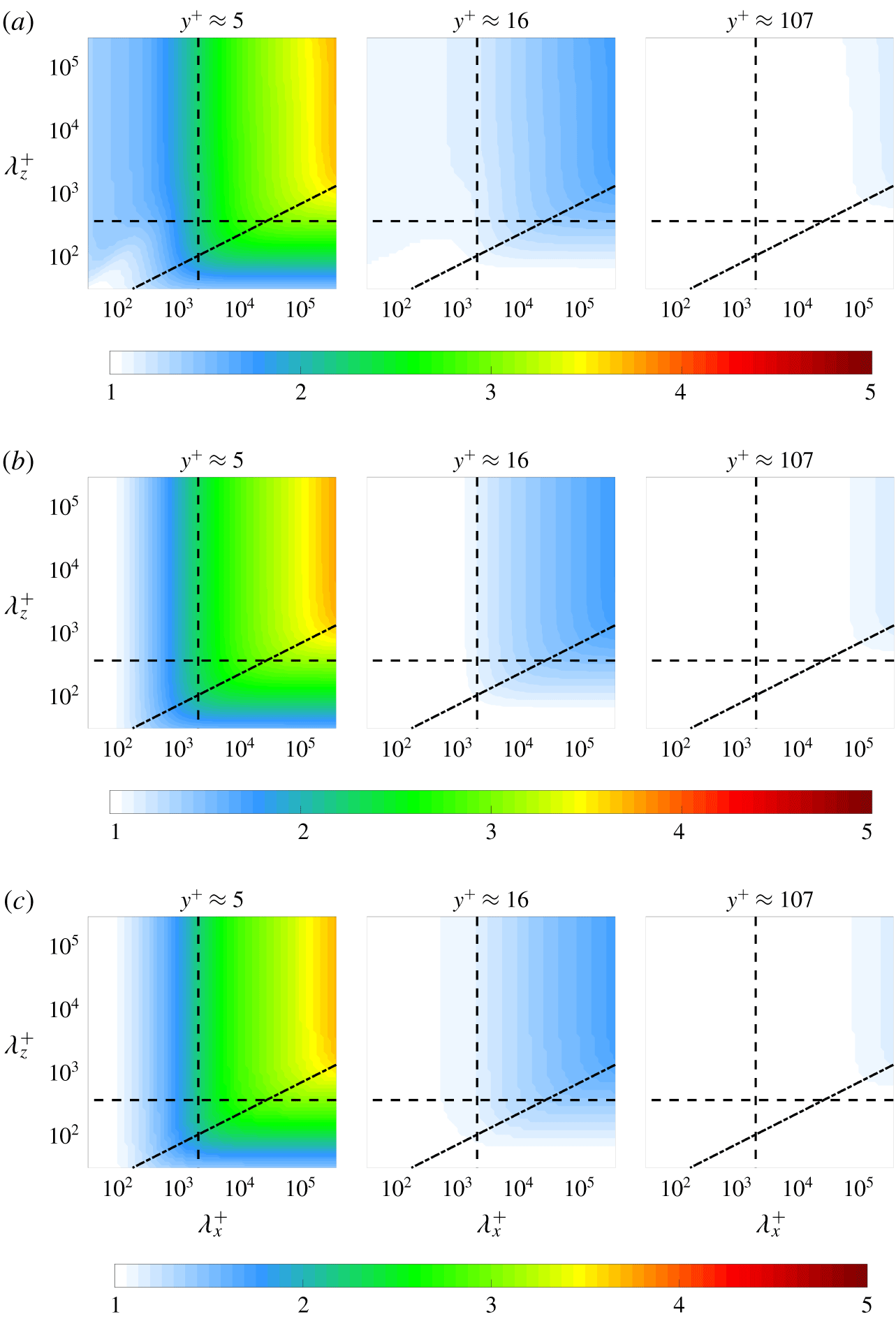
To gain more insight into the effect of each term, we next compute the convective velocities by neglecting the contribution of different terms in the linear dynamics that form the spatio-temporal transfer function in (3.4). In each case, we first describe how neglecting the term(s) of interest alters these operators and then evaluate the effect on the convective velocity. Setting the mean shear term to zero reduces the linear operator in (3.2) to

(7.3)$$\begin{eqnarray}{\mathcal{L}}:=\left[\begin{array}{@{}cc@{}}\displaystyle \left(\text{i}k_{x}(\bar{u}-c)-\frac{1}{Re_{\unicode[STIX]{x1D70F}}}\hat{\unicode[STIX]{x0394}}\right)\unicode[STIX]{x1D644}_{3\times 3} & \hat{\unicode[STIX]{x1D735}}\\ \hat{\unicode[STIX]{x1D735}}^{\text{T}} & 0\end{array}\right].\end{eqnarray}$$

In this case, the operators ${\mathcal{B}}$ and ${\mathcal{C}}$ in (3.8) remain the same. We note that although the mean shear term is zero, $\bar{u}(y)$ is still a function of wall-normal location; therefore there is still shear imposed by the mean flow. Figure 12(a) shows that the convective velocities of the large scales continue to deviate from the mean velocity even when we eliminate the linear term associated with the mean shear. However, the knee occurring at $\unicode[STIX]{x1D706}_{z}^{+}=\frac{5}{2}\sqrt{\unicode[STIX]{x1D706}_{x}^{+}}$ shown in figure 12(a) is different from that at $\unicode[STIX]{x1D706}_{z}^{+}={\unicode[STIX]{x1D706}_{x}^{+}}^{2/3}$ in figure 4 based on the full linear approach. This is consistent with figure 11(b), which indicates that the mean shear term plays a role in the self-similarity predicted in this approach.

We next isolate the role of the pressure. For this analysis we group the effect of the pressure gradient and the mass conservation terms because they both contribute to the non-locality of the turbulent flow. This relationship can be understood by viewing the pressure in the momentum equation as the Lagrange multiplier that enforces the divergence-free velocity field; see e.g. § 5.6.2 in Schmid & Henningson (Reference Schmid and Henningson2001). Neglecting both the pressure term and the divergence-free constraint reduces the operators in the input–output map ${\mathcal{G}}_{\hat{u} ^{\prime }}={\mathcal{C}}_{\hat{u} ^{\prime }}{\mathcal{L}}^{-1}{\mathcal{B}}$ to

(7.4a-c)$$\begin{eqnarray}{\mathcal{C}}_{\hat{u} ^{\prime }}:=\left[\begin{array}{@{}cc@{}}1 & \mathbf{0}_{1\times 2}\end{array}\right]\!,\quad {\mathcal{L}}:=\left[\begin{array}{@{}c@{}}\displaystyle \left(\text{i}k_{x}(\bar{u}-c)-\frac{1}{Re_{\unicode[STIX]{x1D70F}}}\hat{\unicode[STIX]{x0394}}\right)\unicode[STIX]{x1D644}_{3\times 3}+\frac{\text{d}\bar{u}}{\text{d}y}\unicode[STIX]{x1D64E}\end{array}\right]\!,\quad {\mathcal{B}}:=\unicode[STIX]{x1D644}_{3\times 3}.\end{eqnarray}$$

The resulting convective velocities in figure 12(b) are similar to those in figure 12(a) with the mean shear term set to zero. Neither of these terms appear to be responsible for the influence of the large-scale structures that leads to the observed behaviour of the convective velocity in the near-wall region. They also do not reproduce the $\unicode[STIX]{x1D706}_{z}^{+}={\unicode[STIX]{x1D706}_{x}^{+}}^{2/3}$ scaling, but they do emit self-similar structures with a different scaling exponent, $\unicode[STIX]{x1D706}_{z}^{+}=\frac{5}{2}{\unicode[STIX]{x1D706}_{x}^{+}}^{1/2}$.

Figure 13.

Power spectral density of streamwise velocity fluctuations $(\unicode[STIX]{x1D6F7}_{\hat{u} ^{\prime }}(y;k_{x},k_{z},c))/(\max _{c,y}(\unicode[STIX]{x1D6F7}_{\hat{u} ^{\prime }}(y;k_{x},k_{z},c)))$ over wall-normal location $y^{+}$ and phase speed $c$ at $Re_{\unicode[STIX]{x1D70F}}=1000$ from model (7.5) for representative large-scale structures ${\vartriangleleft}(\unicode[STIX]{x1D706}_{x}^{+},\unicode[STIX]{x1D706}_{z}^{+})=(133\,052,857)$, ${\vartriangleright}(\unicode[STIX]{x1D706}_{x}^{+},\unicode[STIX]{x1D706}_{z}^{+})\approx (133\,052,14\,756)$ and intermediate-scale structures $\triangle \;(\unicode[STIX]{x1D706}_{x}^{+},\unicode[STIX]{x1D706}_{z}^{+})\approx (2746,14\,756)$. The colour is in base 10 logarithmic scale. The black solid lines represent the mean streamwise velocity profile, and the black dashed lines are convective velocities, which are defined in (3.7) as the phase speed that maximizes the PSD of the streamwise fluctuations $\unicode[STIX]{x1D6F7}_{\hat{u} ^{\prime }}(y;k_{x},k_{z},c)$.

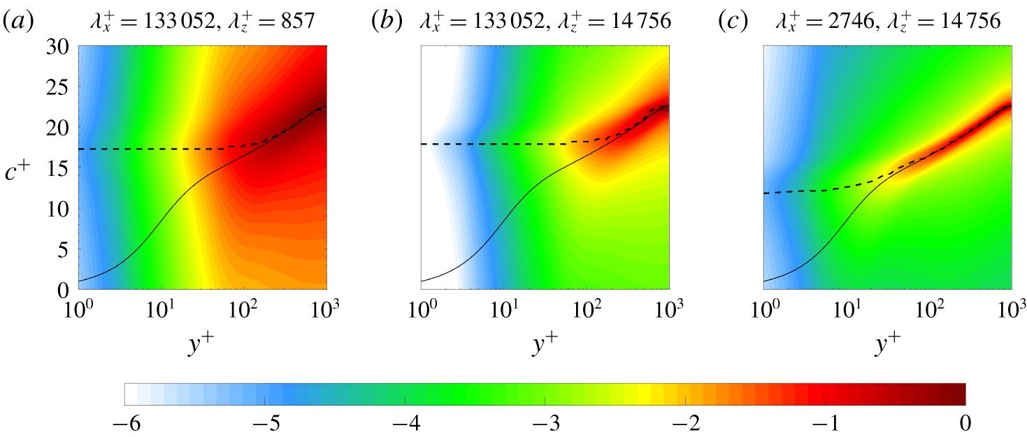
In order to evaluate their combined effect, we next neglect the contributions of both the mean shear and pressure terms, leaving only the advective and viscous terms. The resulting input–output based approach for the streamwise velocity fluctuations is given by $\hat{u} ^{\prime }={\mathcal{C}}_{\hat{u} ^{\prime }}{\mathcal{L}}^{-1}{\mathcal{B}}\hat{f}_{x}$ with

(7.5a-c)$$\begin{eqnarray}{\mathcal{C}}_{\hat{u} ^{\prime }}:=\left[\begin{array}{@{}c@{}}1\end{array}\right]\!,\quad {\mathcal{L}}:=\left[\begin{array}{@{}c@{}}\displaystyle \text{i}k_{x}(\bar{u}-c)-\frac{1}{Re_{\unicode[STIX]{x1D70F}}}\hat{\unicode[STIX]{x0394}}\end{array}\right]\!,\quad {\mathcal{B}}:=\left[\begin{array}{@{}c@{}}1\end{array}\right].\end{eqnarray}$$

Figure 12(c) shows the resulting convective velocity contours, which are similar to the results in panels (a,b). In particular, they reproduce the influence of the large-scale structures in the near-wall and buffer regions seen in the full LNS based approach. Figure 13 plots the power spectral density of the streamwise velocity fluctuations at different phase speeds $c^{+}$ and wall-normal locations $y^{+}$ computed using the model in (7.5). Although there are some differences from the results obtained using the full LNS system shown in figure 5, the phase speed that maximizes the energy spectrum, i.e. the convective velocity, still asymptotes to a constant value near the wall for large wavelength structures.

The main difference between these results and the full LNS based approach is that they show the same $\unicode[STIX]{x1D706}_{z}^{+}=\frac{5}{2}{\unicode[STIX]{x1D706}_{x}^{+}}^{1/2}$ scaling as the previous model in (7.5) with the influence of the pressure and mean shear removed. The inability to reproduce the correct aspect ratio for the self-similar structures suggest that their morphology is due to interactions between viscous mechanisms and other inviscid mechanisms arising due to the interaction of the fluctuations with the mean shear $\text{d}\bar{u}/\text{d}y$ and the pressure, such as the lift-up effect (Brandt Reference Brandt2014) and the Orr mechanism (Farrell Reference Farrell1987; Jiménez Reference Jiménez2013). However, the prediction of the main trends and scale interactions suggest that this type of model may provide a good balance between accuracy and simplicity. We next explore its potential as a viscous correction to Taylor’s hypothesis.

We obtain this correction by rewriting (7.5) as

(7.6)$$\begin{eqnarray}\text{i}k_{x}(\bar{u}(y)-c)\hat{u} ^{\prime }-\frac{\hat{\unicode[STIX]{x0394}}}{Re_{\unicode[STIX]{x1D70F}}}\hat{u} ^{\prime }=\hat{f}_{x}.\end{eqnarray}$$

Figure 14 compares the average convective velocity of streamwise velocity fluctuations computed using the viscous correction (7.6) with its corresponding weighting functions $h=\langle |{\mathcal{F}}_{xz}(u^{\prime })|^{2}\rangle k_{x}^{2}$ and an averaging domain of $(\unicode[STIX]{x1D706}_{x}^{+},\unicode[STIX]{x1D706}_{z}^{+})>(500,80)$ at $Re_{\unicode[STIX]{x1D70F}}=1000$ to the results from the full LNS based approach and convective velocities obtained from DNS data at $Re_{\unicode[STIX]{x1D70F}}=932$ from Geng et al. (Reference Geng, He, Wang, Xu, Lozano-Durán and Wallace2015). This figure shows that the average convective velocity predicted from the viscous correction shows excellent agreement with results obtained from DNS data for $y^{+}\in [5,15]$, but begins to deviate for $y^{+}\lesssim 3$. We therefore conclude that this viscous correction provides a potential dynamical modification on Taylor’s hypothesis to improve the convective velocity estimates for use with experimental data.

This viscous correction introduced in (7.6) could be augmented using an eddy viscosity, in the spirit of the eddy viscosity enhanced LNS equations introduced in Reynolds & Hussain (Reference Reynolds and Hussain1972). Such a dynamical correction was previously shown to provide similar improvements in model-fidelity for certain structures as the inclusion of coloured-in-time forcing (Zare et al. Reference Zare, Jovanović and Georgiou2017). This type model enhancement may be particularly relevant in this context because the pertinent terms would all be retained in the associated modification of the viscous correction proposed in (7.6). Assessing the potential benefits of such an approach is a topic of future work.

Figure 14.

The average convective velocity of streamwise velocity fluctuations, $[u_{c}]_{h}^{+}(y)$: (▫, blue), computed using the viscous correction (7.6) with their corresponding weighting functions $h=\langle |{\mathcal{F}}_{xz}(u^{\prime })|^{2}\rangle k_{x}^{2}$ and an averaging domain of $(\unicode[STIX]{x1D706}_{x}^{+},\unicode[STIX]{x1D706}_{z}^{+})>(500,80)$ at $Re_{\unicode[STIX]{x1D70F}}=1000$. Results are plotted with convective velocities of streamwise velocity fluctuations computed from both the LNS based approach described herein for $Re_{\unicode[STIX]{x1D70F}}=1000$: (▵, red) and DNS data (Geng et al. Reference Geng, He, Wang, Xu, Lozano-Durán and Wallace2015) at $Re_{\unicode[STIX]{x1D70F}}=932$: (——, red). The black dashed line is the turbulent mean velocity profile at $Re_{\unicode[STIX]{x1D70F}}\approx 1000$ from Lee & Moser (Reference Lee and Moser2015).

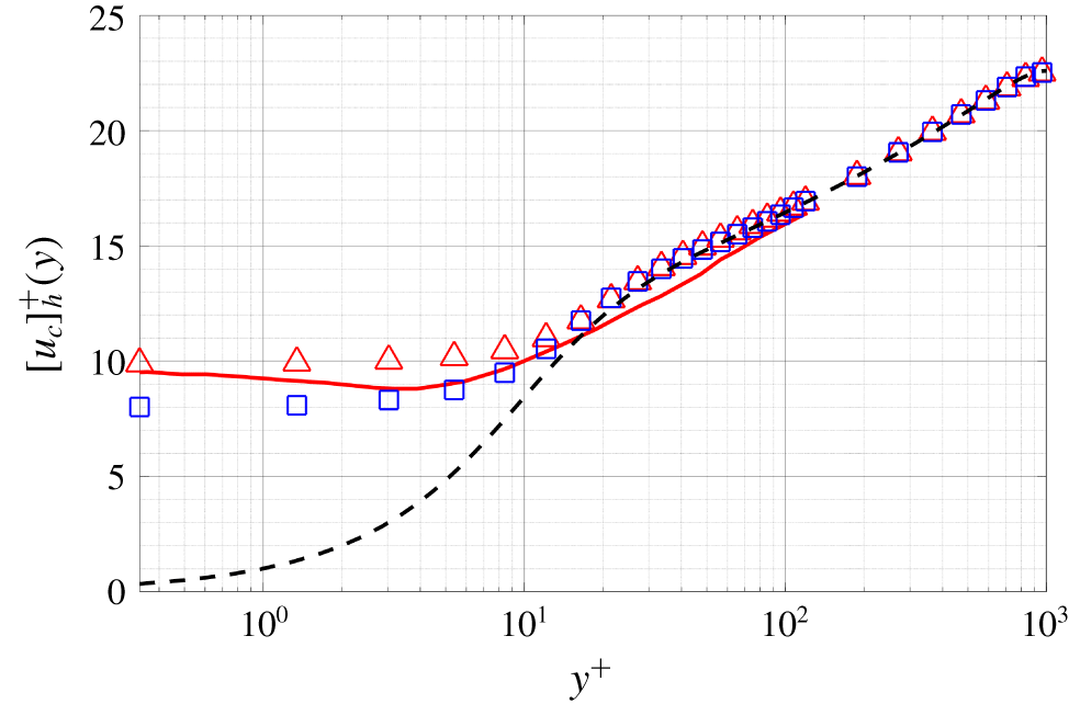
The convective velocities computed with this viscous correction to Taylor’s hypothesis for a range of Reynolds numbers are compared in figure 15. The results indicate that the regions in ($\unicode[STIX]{x1D706}_{x}^{+}$, $\unicode[STIX]{x1D706}_{z}^{+}$) where the convective velocities deviate from the local mean velocity are very similar across these Reynolds numbers, which is consistent with the observations in figure 4 indicating that the viscous correction preserves the previously observed Reynolds number invariance.

Figure 15.

$u_{c}(y,\unicode[STIX]{x1D706}_{x},\unicode[STIX]{x1D706}_{z})/\bar{u}(y)$ predicted using the viscous correction to Taylor’s hypothesis in (7.6) at (a) $Re_{\unicode[STIX]{x1D70F}}=550$, (b) $Re_{\unicode[STIX]{x1D70F}}=1000$ and (c) $Re_{\unicode[STIX]{x1D70F}}=5200$. The black dashed lines are given by $(\unicode[STIX]{x1D706}_{x},\unicode[STIX]{x1D706}_{z})=(2,0.4)$. The black dash-dot lines are $\unicode[STIX]{x1D706}_{z}^{+}=\frac{5}{2}\sqrt{\unicode[STIX]{x1D706}_{x}^{+}}$, which fit through the knee of these contours.

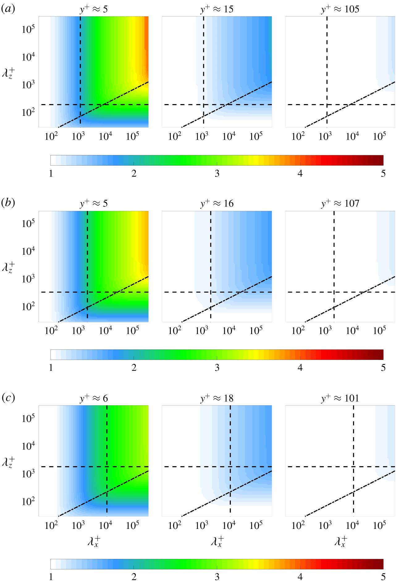
The viscous correction proposed here may also be applicable to input–output based computations of convective velocities for other fluctuating quantities due to the similarity in the behaviour of the near-wall convective velocities of velocity and vorticity components previously reported in the literature; see e.g. figures 3 and 5 of Geng et al. (Reference Geng, He, Wang, Xu, Lozano-Durán and Wallace2015), figures 1 and 2 of Kim & Hussain (Reference Kim and Hussain1993) and the results in Liu & Gayme (Reference Liu and Gayme2019). Exploring this notion is a topic of ongoing work.