Implications
Incorporating the longevity trait as selection criteria should result in an improvement of the herd profitability. However, it is extremely important to define a model that maximizes the prediction accuracy of breeding values. In this sense, this study has provided two main results: (1) excluding censored data from the genetic evaluation of longevity may have an unfavorable impact on the selection of top animals, and (2) the Weibull frailty hazard model (WM) seems to be a better option to evaluate longevity in Nellore cattle when comparing with linear models. These results could contribute to the longevity genetic evaluation in beef cattle.
Introduction
The reproductive performance of beef cattle is an important aspect of the beef production chain, affecting the profitability of the production system and prices paid by the consumer. Furthermore, the reproductive performance of herds limits the genetic gain of the population, as low reproduction rates affect the generation interval and selection intensity adopted in breeding programs (Van Arendonk, Reference Van Arendonk1986; Van Melis et al., Reference Van Melis, Eler, Rosa, Ferraz, Figueiredo, Matos and Oliveira2010a).
Longevity can be used as selection criterion of cows aiming to increase their reproductive potential. Maximization of this criterion allows reducing the rate of involuntary culling, with a consequent reduction in replacement costs and an increase in the number of productive animals, which is expected to improve the overall profitability (Van Arendonk, Reference Van Arendonk1986; Neves et al., Reference Neves, Carvalheiro and Queiroz2012). Different approaches have been used to evaluate longevity in Nellore cattle, in which phenotypic expression is evaluated using discrete variable as stayability or number of calvings (Silva et al., Reference Silva, Eler, Ferraz, Golden and Oliveira2003 and Reference Silva, Formigoni, Eler and Ferraz2006; Van Melis et al., Reference Van Melis, Eler, Rosa, Ferraz, Figueiredo, Matos and Oliveira2010a and Reference Van Melis, Oliveira, Eler, Ferraz, Casellas and Varona2010b; Neves et al., Reference Neves, Carvalheiro and Queiroz2012), or continuous variables as productive life or age of cow at last calving (Mercadante et al., Reference Mercadante, Lôbo and Oliveira2000; Caetano, Reference Caetano2011).
When the longevity is evaluated on a continuous scale, only the partial expression of longevity of some cows is known, as part of the females remain productive at the time of genetic evaluation or were culled involuntary due to reasons that are not related to reproductive efficiency. These partial records are termed as censored records. According to Hou et al. (Reference Hou, Madsen, Labouriau, Zhang, Lund and Su2009), the use of these phenotypes as uncensored or their exclusion from genetic analysis might lead to biased prediction of breeding values for sires with a large number of daughters with censored records. However, the adequate inclusion of these observations in genetic evaluations could avoid distorted inferences and improve breeding value predictions (Guo et al., Reference Guo, Gianola and Short2001).
Therefore, the aim of the present study was to evaluate the prediction ability of models that cope with longevity phenotypic expression as uncensored and censored in order to determine the most appropriate model for the genetic analysis of this trait in Nellore breed.
Material and methods
Data
The data set used in this study came from Nellore Alianca database, which contains data from different Nellore breeding programs. Here, there were considered information of 82 304 Nellore cows, born between 1993 and 2007, and which had records of age at first calving. The animals were from 171 herds located in the south-east and mid-west regions of Brazil.
The animals were managed on pasture with mineral supplementation and the reproductive management of multiparous cows consisted of a summer breeding season, which ranged from November to January. Pregnancy test was performed 60 days after the breeding season and those cows which did not get pregnant were culled.
Longevity was defined as the difference between the dates of last weaned calf and cow birth. Females with incomplete weaning data of their progenies (4818 cows) and longevity lower than 30 months (124 cows) were excluded from the analysis. Subsequently, 77 353 females remained in the data set, including 61 097 cows with uncensored phenotypic information and 16 256 cows with censored records, as their offspring were born in the 2010 season.
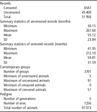
The contemporary groups were defined by the combination of year, season, month and farm of birth, farm and management group at weaning, farm and management group at long-yearling, and precocity. Animals with age at first calving lower than 30 months were defined as precocious. Only females belonging to contemporary groups with more than five cows with uncensored records remained in the analyses. Therefore, records of 15 688 cows with phenotypic information and 9709 cows which still being productive were excluded. The complete description of the data structure is shown in Table 1.
Descriptive summary of the data set used in the analysis of longevity

Statistical models
In the Gaussian linear model (LM), only uncensored records were considered. This model can be written as following:
 $${\bf{y}} \,{\equals}\,{\bf X\bbeta} {\plus}{\bf{Zu}} {\plus}{\bf{e}} $$
where y is the vector of longevity observations; β the vector of contemporary group effects; u the vector of breeding values, assuming
 ${\bf u} \sim\! {N}\left( {0,{\rm }{\bf A}{\rm \sigma }_{{u}}^{2} } \right)$
, where A and
 ${\rm \sigma }_{{u}}^{2} $
are the numerator relationship matrix and additive genetic variance, respectively; e the vector of residuals, which were assumed to follow a normal distribution with homoscedastic variance, that is
 ${\bf e}\!\sim\! {N}\left( {0,{\rm }{\bf I}{\rm \sigma }_{{e}}^{2} } \right)$
, where I and
 ${\rm \sigma }_{{e}}^{2} $
are the identity matrix and residual variance, respectively.
The censored Gaussian linear model (CLM) is similar to LM. However, in this case, a partition containing censored records is included in the vector of observations:
 $$\left( {\matrix{ {{\mib{y}} _{{{\mib{unc}} }} } \cr {{\mib{y}} _{{\mib{c}} } } \cr } } \right)\,{\equals}\,{\bf X\bbeta} {\plus}{\bf{Zu}} {\plus}{\bf{e}} $$
where y unc and y c correspond to uncensored observations of longevity and the augmented records for censored females, respectively.
In CLM, the data augmentation methodology (Tanner and Wong, Reference Tanner and Wong1987) is applied to cope with censored records. The joint conditional distribution of uncensored ( y unc ) and censored ( y c ) observations can be represented as following (Sorensen et al., Reference Sorensen, Gianola and Korsgaard1998; Guo et al., Reference Guo, Gianola and Short2001):
 $$\eqalignno{ p\left( {y\!\mid\!\beta ,u,\sigma _{e}^{2} } \right){\equals}& \left( {2\pi \sigma _{e}^{2} } \right)^{{{\minus}{\raise0.7ex\hbox{$n$} \!\mathord{\left/ {\vphantom {n 2}}\right.\kern-\nulldelimiterspace}\!\lower0.7ex\hbox{$2$ }}}} {\rm exp} \left\{ {{\minus}{1 \over {2\sigma _{e}^{2} }}}\left [ \sum\limits_{i{\equals}1}^m \left( {y_{{unc_{i} }} {\minus}x_{i}^{'} \beta {\minus}z_{i}^{'} u} \right) \right \right \cr&\plus \left \left \mathop \sum\limits_{i{\equals}m{\plus}1}^n \left( {y_{{c_{i} }} {\minus}x_{i}^{'} \beta {\minus}z_{i}^{'} u} \right)} \right]} \right\}$$
where m and n are, respectively, the number of uncensored observations and the total number of records and c i the censored phenotype of longevity adopted for ith female.
The censored longevity records ( y c ) are drawn in each iteration of Gibbs sampling using a fully conditional posterior truncated normal distribution (Sorensen et al., Reference Sorensen, Gianola and Korsgaard1998; Cardoso et al., Reference Cardoso, Rosa, Tempelman and Torres Junior2009), which can be written as following:
 $$\eqalignno{ p&\left( {y_{{c_{i} }} \!\mid\!\beta ,u,\sigma _{u}^{2} ,\sigma _{e}^{2} ,y_{{unc}} ;y_{{c_{i} }} \,\gt\,c_{i} } \right)\,{\equals}{{\phi _{{y_{{c_{i} }} }} \left( {x_{i}^{'} \beta {\plus}z_{i}^{'} u_{i} ,\sigma _{e}^{2} } \right)} \over {1{\minus}\Phi \left( {{{c_{i} {\minus}x_{i}^{'} \beta {\minus}z_{i}^{'} u_{i} } \over {\sigma _{e} }}} \right)}}$$
where ϕ(.) and Φ(.) are the density and cumulative normal distribution functions, respectively and c i the truncation point, which is the partial observation of longevity of the ith cow.
The following WMWM was also applied to evaluate longevity (Ducrocq and Casella, Reference Ducrocq1996):
 $$h\left( {LONG} \right)\,{\equals}\,\lambda _{0} \left( {LONG} \right){\rm exp}\left( {X\beta {\plus}W\theta {\plus}Zs} \right)$$
where h(LONG) is the hazard function; λ
0(LONG) the Weibull baseline hazard function, in which λ
0=λρ(LONG)
ρ−1 where λ and ρ are the scale and shape parameters, respectively; β the vector of time-independent systematic effects of the contemporary groups; θ the time-dependent effect of period, which will be defined subsequently; s the time-independent random effect of sire, which was assumed to follow a multivariate normal distribution with 0 mean and variance and covariance matrix
 $A_{s} \sigma _{s}^{2} $
where A
s
and
 $\sigma _{s}^{2} $
are the numerator relationship matrix between sires and sire variance, respectively.
The sire model described in equation (5) was used to estimate sire variance and this component was multiplied by four to obtain the additive genetic variance. Subsequently, this variance component was considered as known for the prediction of breeding values on the basis of standard animal model, which were assumed to follow a multivariate normal distribution with 0 mean and variance and covariance matrix
 ${A}\sigma _{u}^{2} $
, where A and
 $\sigma _{u}^{2} $
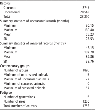
are the numerator relationship matrix between animals and additive genetic variance, respectively. The data editing was performed as described for the whole data set, but also including an additional restriction: only cows with known parents were considered in the Weibull frailty hazard sire model (Table 2).
Descriptive summary of the data set used in the frailty Weibull Hazard sire model for longevity analysis

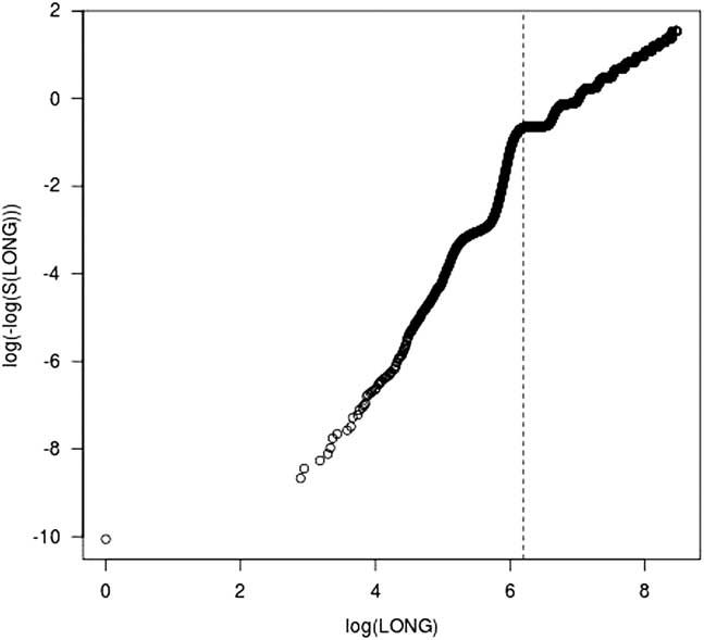
The assessment of the adequacy of Weibull distribution as base hazard function was performed graphically by plotting log(LONG) v.
 ${\rm log}\big[ {{\minus}{\rm log}\big( {\hat{S}\big( {LONG} \big)} \big)} \big]$
(Figure 1), where log is the natural logarithm and
 $\hat{S}\left( . \right)$
is Kaplan–Meyer survival function estimation. In Figure 1, linearity is not observed in the whole period for LONG, however there are two periods in which linearity could be approximated and within each of these periods the assumption of Weibull model could be reasonable. Therefore, the periods, defined as time-dependent effects, were from 0 to 46.38 months and >46.38 months. The practical implication of cut points definition are periods in which different Weibull baseline hazard are modeled to avoid large deviations from the assumption that culling probability remains constant over the whole life of an animal (Ducrocq, Reference Ducrocq and Casella2005).
Graphical assessment of the Weibull hazard function adequacy for longevity (LONG). The survival function estimate,
 $\hat{S}\left( . \right)$
, was obtained using the Kaplan–Meier estimator and the vertical line delimit periods considered for LONG, which are from 0 to 46.38 and >46.38 months.

The GIBBS1F90 and GIBBS2CEN programs (Misztal et al., Reference Misztal, Tsuruta, Strabel, Auvray, Druet and Lee2002) were applied for LM and CLM analysis, respectively. Initially, three chains of 500 000 iterations were obtained, where in the initial values for variance components corresponded to heritabilities of 0.10, 0.40 and 0.80. Graphical inspection and test of Brooks, Gelman and Rubin (Gelman and Rubin, Reference Gelman and Rubin1992) and Heldelberger and Welch were performed (Heldelberger and Welch, Reference Heldelberger and Welch1983) using the coda package in R (R Core Team, 2013), all of which indicating that convergence was achieved. Only one of the chains was used for inference, considering a burn-in period of 50 000 and 100 000 samples for LM and CLM, respectively. On the other hand, the Survival Kit v6.0 software (Ducrocq et al., Reference Ducrocq, Sölkner and Meszaros2010) was used for WM.
Model comparison
The association among model breeding value predictors and agreement in ranking, between the three models applied, were evaluated by computing Spearman’s correlation and the top 10% of bulls (TOP10%) in common, considering only those with more than 10 daughters with uncensored records. In addition, the accuracy of sire breeding values was calculated using the following equation for the linear models (Korsgaard et al., Reference Korsgaard, Andersen and Jensen2002):
 $$r\,{\equals}\,\sqrt {1{\minus}{{\rm PEV} \over {\sigma _{u}^{2} }}} $$
where
 $\sigma _{u}^{2} $
is the additive genetic variance and PEV the prediction error variance, which was calculated as follows:
 $${\rm PEV}\,{\equals}\,{{\sum_{i{\equals}1}^{ns} u_{i}^{2} {\minus}{{\left( {\sum_{i{\equals}1}^{ns} u_{i} } \right)^{2} } \over {ns}}} \over {ns}}$$
where u i is the ith breeding value sample drawn from the conditional posterior distribution of breeding value of the ith sire and ns the number of samples kept after burn-in period.
On the other hand, the accuracy of the WM model was calculated using the following equation (Ducrocq, Reference Ducrocq and Casella2005):
 $$r\,{\equals}\,\sqrt {{{n{\times}h^{2} } \over {\left( {n{\minus}1} \right)h^{2} {\plus}4}}} $$
where n is the number of uncensored daughters per sire and h 2 the heritability, which was estimated as following (Yazdi et al., Reference Yazdi, Visscher, Ducrocq and Thompson2002):
 $$h^{2} \,{\equals}\,{{4\sigma _{s}^{2} } \over {\sigma _{s}^{2} {\plus}1}}$$
The data set used for analysis was divided into training and validation sets, containing 80% and 20% of the records, respectively. This process was performed randomly in 10 repetitions applying the following restrictions: (a) at least three animals per contemporary group in the training set; (b) sires with more than 10 progenies with uncensored records (352 sires) should have daughters in the training and validation sets. The variance components estimated using the whole data set in each model were used as true values in the prediction of breeding values of the animals in the training set.
The prediction ability comparisons explored χ 2 statistics between observed and expected classes of longevity, considering progenies of sires with more than 10 uncensored daughters. For this purpose, the phenotypes of longevity were categorized using 72 months as the truncation point, as typically applied to stayability evaluations (Silva et al., Reference Silva, Eler, Ferraz, Golden and Oliveira2003 and Reference Silva, Formigoni, Eler and Ferraz2006; Van Melis et al., Reference Van Melis, Eler, Rosa, Ferraz, Figueiredo, Matos and Oliveira2010a). Then, daughters probabilities for LONG in each category were estimated using logistic regression of daughters frequency on sire expected progeny difference from training set. The estimated probabilities were used to predict frequency of censored and uncensored progenies in the testing data. Finally, the sum of χ 2 over sires for two fertility events was computed as following:
 $$\chi ^{2} \,{\equals}\,\mathop \sum\limits_{i{\equals}1}^{nt} \mathop \sum\limits_{j{\equals}1}^2 {{\left( {O_{{ij}} {\minus}E_{{ij}} } \right)^{2} } \over {E_{{ij}} }}$$
where O ij and E ij are the number of observed and expected phenotypes of daughters of the sire i to be into a jth class of LONG and nt the total number of sires.
Results and discussion
In the present study, the shape parameter of the Weibull distribution
 $\left( {\hat{\rho }} \right)$
obtained was 2.63±0.01. This parameter indicates whether the phenotypic expression of a trait decreases, remains constant or increases with increasing over time, when
 $\hat{\rho }\,\lt\,1$
,
 $\hat{\rho }\,{\equals}\,1$
and
 $\hat{\rho }\,\gt\,1$
, respectively. Similar
 $\hat{\rho }$
(2.45±0.03) was reported by Caetano (Reference Caetano2011), who studied longevity of Nellore females defined as the difference between the date of last calving and cow birth.
The heritability estimates
 $\big( {\hat{h}^{2} } \big)$
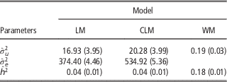
obtained with the LM (0.04) and CLM (0.04) models showed low magnitude; being much lower than that achieved using the WM (0.18) model (Table 3). This is an indicative that censored records represent a large amount of the population longevity genetic variability and, comparing with linear models, the survival analysis seems to be the best way to capture the genetic variation for longevity trait in this Nellore population. This pattern of results was also reported by Lubbers et al. (Reference Lubbers, Brotherstone, Ducrocq and Visscher2000) in the evaluation of longevity as a discrete trait in dairy cattle. According to these authors, the
 $\hat{h}^{2} $
obtained with WM was 0.17 and only 0.05 with the LM model.
Posterior mean and standard deviation (in parentheses) of genetic variance
 $\left( {\hat{\sigma }_{u}^{2} } \right)$
, residual variance
 $\left( {\hat{\sigma }_{e}^{2} } \right)$
and heritability
 $\left( {\hat{h}^{2} } \right)$
for longevity (LONG) using different models

LM=Gaussian linear model; CLM=censored Gaussian linear model; WM=Weibull frailty hazard model.
In general, survival models have provided higher
 $\hat{h}^{2} $
for longevity than linear models (Ducrocq et al., Reference Ducrocq, Boichard, Barbat and Larroque1988; Lubbers et al., Reference Lubbers, Brotherstone, Ducrocq and Visscher2000; Caraviello et al., 2004; Forabosco et al., Reference Forabosco, Bozzi, Filippini, Boettcher, Van Arendonk and Bijma2006; Raguž et al., Reference Raguž, Jovanovac, Mészáros and Sölkner2014). Even for other censored traits as days to calving, days from calving to first insemination and days open, the survival analysis, usually, estimates higher
 $\hat{h}^{2} $
compared with linear approaches, whereas similar heritability estimates are obtained with LM and CLM models (Donoghue et al., Reference Donoghue, Rekaya and Bertrand2004a and Reference Donoghue, Rekaya and Bertrand2004b; Hou et al., Reference Hou, Madsen, Labouriau, Zhang, Lund and Su2009; Garcia et al., Reference Garcia, Rosa, Valente, Carvalheiro and Albuquerque2016). Our results were similar to those from Mercadante et al. (Reference Mercadante, Lôbo and Oliveira2000) which found low
 $\hat{h}^{2} $
(0.08) using LM model and to the low to moderate
 $\hat{h}^{2} $
(0.25) presented by Caetano (Reference Caetano2011) using WM model.
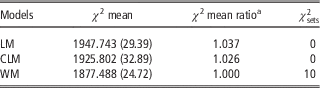
The WM model showed the best prediction ability, providing the lowest χ 2 average and the highest number of sets in which a model had the smallest value of χ 2 statistics (Table 4). In contrast, the CLM and LM models showed prediction abilities which were, respectively, 2.6% and 3.7% less efficient than WM. These results corroborates with Caraviello et al. (2004) which observed more accurate predictions for longevity in US Holstein applying survival analysis than linear model.
 ${\chi}\,^2$
mean, standard deviation (in parenthesis),
 ${\chi}\,^2$
mean ratio and number of repetitions in which different models showed the best prediction ability
 $\left( {\chi _{{{\rm sets}}}^{\,{\rm 2}} } \right)$
for longevity

LM=Gaussian linear model; CLM=censored Gaussian linear model; WM=Weibull frailty hazard model.
a It was calculated as a ratio between each model mean and best χ 2 observed mean.
Similarly, González-Recio et al. (Reference González-Recio, Chang, Gianola and Weigel2006) reported a higher efficiency of the MW model in predicting pregnancy at two early stages of lactation. Hou et al. (Reference Hou, Madsen, Labouriau, Zhang, Lund and Su2009) found a better prediction ability of the WM model compared with the CLM model, evaluating days from calving to first insemination in dairy cattle. Considering the same Nellore population analyzed here, Garcia et al. (Reference Garcia, Rosa, Valente, Carvalheiro and Albuquerque2016) reported that the WM model provided the best prediction ability for age at first calving.
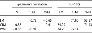
The association between breeding values predicted with the LM and CLM models were 0.78 and 0.82, respectively, considering all sires and sires with more than 10 uncensored progenies (Table 5). Similar association strength were reported by Donoghue et al. (Reference Donoghue, Rekaya and Bertrand2004b), who obtained Pearson’s correlations of 0.81 and 0.84 between predictions obtained with the LM and CLM models, respectively, taking into account all sires and sires with more than 20 daughters.
Spearman’s correlation between breeding value predictions and percentage of best bulls in common (TOP10%), considering all sires (above diagonal) and the sires with at least 10 daughters with uncensored records (below diagonal)Footnote a , from different models for longevity

LM=Gaussian linear model; CLM=censored Gaussian linear model; WM=Weibull proportional hazard model.
a 1256 and 352 sires.
The associations between predictions obtained with CLM and WM for the two situations designed were higher than those obtained between CLM and LM (Table 5). Pereira et al. (Reference Pereira, Oliveira, Eler, Silva and Van Melis2007), studying age at first conception of Nellore heifers, reported higher and moderate associations, −0.99 and −0.72, when breeding values of all sires and TOP10% sires were considered, respectively. On the other hand, Hou et al. (Reference Hou, Madsen, Labouriau, Zhang, Lund and Su2009), studying days from calving to first insemination in dairy cattle reported a correlation of −0.92 between the breeding values predicted with CLM and WM, which was similar to the results here presented. In survival models, covariates are modeled multiplicatively to the base hazard function using an exponential link function, as in expression (5). Then, the more positive the breeding value, the lower the hazard function, which indicated individuals with most desirable greater genetic merit. Hence, the correlation between breeding value predictions of linear models and the WMs are expected to be negative.
The LM and WM models provided the weakest associations between predicted sire breeding values, −0.65 and −0.66 (Table 5). Similarly, Caraviello et al. (2004), analyzing longevity in US Holstein, observed sire breeding value associations ranging from −0.71 to −0.73 between LM and WM models. Other similar result was reported by González-Recio et al. (Reference González-Recio, Chang, Gianola and Weigel2006), who investigated days open in Holstein cattle and obtained Spearman’s correlation of −0.65 between sire breeding values predicted with the LM and WM models.
The percentages of bulls in common, considering only 10% of sires with the highest breeding values, were around 75% and 54%, respectively, between LM–CLM and LM–WM models, considering all sires, and 75% between LM–CLM and LM–WM, when only sires with more than 10 progenies with uncensored records were taken into account (Table 5). Thus, there is evidence of some degree of reranking of animals in terms of genetic merit between LM, CLM and WM. Similar results were reported by Donoghue et al. (Reference Donoghue, Rekaya and Bertrand2004b) for LM and CLM, with raking agreement of 62%. Likewise, González-Recio et al. (Reference González-Recio, Chang, Gianola and Weigel2006) reported changes in the ranking of animals for LM–CLM, although a high ranking agreement was observed between CLM and WM.
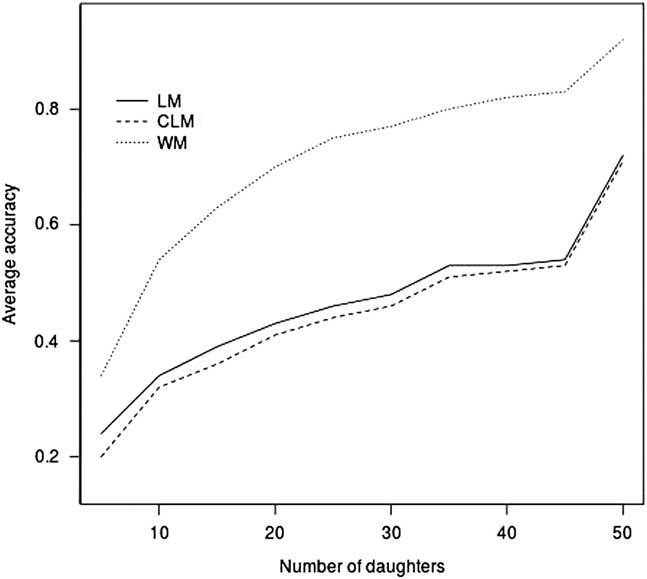
The accuracies of sire breeding values for LM and CLM were similar, but both were lower than those obtained for WM (Figure 2). These differences between the linear models and proportional hazards model might be related to the greater genetic variability observed when the survival analysis model was applied. In contrast, Yazdi et al. (Reference Yazdi, Visscher, Ducrocq and Thompson2002), using simulated data, obtained similar accuracies of sire breeding values predicted by survival and linear models. On the other hand, our results agree with those of Raguž et al. (Reference Raguž, Jovanovac, Mészáros and Sölkner2014) which found higher average sires’ reliabilities for longevity in Simmental cattle using survival analysis than linear model.
Average accuracy of prediction of sire breeding values for longevity (LONG), under different models, as a function of number of uncensored daughters per sire. Sires were grouped considering five progenies per class, except in the last class in which all sires with ⩾50 uncensored progenies were included. LM=Gaussian linear model; CLM=censored Gaussian linear model; WM=Weibull frailty hazard model.

The exclusion of censored data from the genetic evaluation of longevity may have a considerable impact on the selection of top animals, once an important disagreement in the ranking of sires was observed between LM–CLM and LM–WM. qTherefore, the Weibull frailty model would be recommended for genetic evaluation of longevity in this population.
A challenge in the application of Weibull frailty model is related to multivariate analysis. An option would be to use the two-step approach, which is a combination of survival analysis and linear animal model (Ducrocq et al., Reference Ducrocq, Quaas, Pollak and Casella2001). On the other hand, one could consider using piecewise proportional hazard model. In this approach, the inference can be performed exploring a coincidence between likelihood functions of the survival model and a suitable defined generalized linear mixed model (Maia et al., Reference Maia, Madsen and Labouriau2013). This model could be considered in a further investigation in this population.
Conclusion
The model in which censored records of longevity were excluded from the analysis showed the lowest prediction ability of reproductive events of sire progenies. On the other hand, the best predictive performance was obtained when the survival analysis was applied. Therefore, the WM would be recommended to perform genetic evaluation of longevity in this population.
Acknowledgments
The first author was supported by grants (no. 2009/15010-6) from Sao Paulo Research Foundation (FAPESP) and (no. 1817-12-4) from Coordination for the Improvement of Higher Education Personnel (CAPES). The last author thanks the Sao Paulo Research Foundation (FAPESP grant no. 2009/16118-5) for the financial support. The authors are thankful to GenSys Consultores Associados S/S Ltda. for providing the data used in this research.