2. Theory

We consider a gas bubble and a viscoelastic particle surrounded by a viscous incompressible liquid. Both the bubble and the particle are assumed to be spherical at rest. We use two spherical coordinate systems, $(r_{1},\theta _{1},\varepsilon _{1})$ and $(r_{2},\theta _{2},\varepsilon _{2})$ , which are originated at the equilibrium centres of the bubble and the particle, respectively; see figure 1. The direction $\theta _{1}=\theta _{2}=0$ corresponds to the z axis. The distance between the equilibrium centres of the bubble and the particle is denoted by d. Our calculation is based on the theory developed by Doinikov et al. (Reference Doinikov, Regnault, Mauger, Blanc-Benon and Inserra2022) for acoustic microstreaming generated by two interacting oscillating bubbles.

Figure 1.

Coordinate systems used in calculations and calculation flowcharts for the first-order solution (top) and the second-order solution (bottom). Here, $r_{s}$ is the radial coordinate of the disturbed bubble surface, $v^{(1)}$ and $v^{(2)}$ are the first-order liquid velocities generated by the oscillations of the bubble and the particle, respectively, $u$ is the displacement vector inside the particle, $V_{E}$ and $V_{S}$ are, respectively, the Eulerian streaming velocity and the Stokes drift velocity in the liquid.

We assume that in the general case, the bubble undergoes $N$ axisymmetric oscillation modes with mode numbers $M_{1} , M_{2}$ ,…, $M_{N}$ . Then the disturbed surface of the bubble can be represented by

(2.1) \begin{equation} r_{s}=R_{10}+e^{-i\omega t}\sum _{n=M_{1}}^{M_{N}}s_{n}P_{n}\left(\mu _{1}\right) ,\end{equation}

where $r_{s}$ is the radial coordinate of the disturbed bubble surface, $R_{10}$ is the equilibrium radius of the bubble, $\omega$ is the angular oscillation frequency, $P_{n}$ is the Legendre polynomial of degree n, $\mu _{1}=\cos \theta _{1}$ and $s_{n}$ is the complex amplitude of the nth mode of the bubble. The values of $s_{n}$ can be taken from experimental measurements or, in some cases, they can be calculated analytically in terms of the amplitude of the driving acoustic pressure. We assume that the oscillations of the bubble are excited by the driving acoustic pressure, while the oscillations of the particle are excited by the oscillations of the bubble.

The process of the derivation of the second-order mean flow (acoustic streaming) around the bubble–particle system, as well as the calculation of the time-averaged shear stress on the particle surface, is summarised in figure 1 using a flowchart representation. The supposedly known amplitudes of the bubble oscillations are used as input data when deriving the first-order (linear) scattered field in the liquid (the top flowchart in figure 1). In parallel, the first-order scattered field inside the particle is derived using the equation of motion of a viscoelastic medium. The unknown constants of the first-order solution are found using appropriate boundary conditions at the interfaces of the bubble and the particle. At the next stage of the calculation (the bottom flowchart in figure 1), the time-averaged second-order liquid velocity is derived. To this end, the results obtained by Doinikov et al. (Reference Doinikov, Regnault, Mauger, Blanc-Benon and Inserra2022) for the case of two interacting non-sphericallyoscillating bubbles are applied to the bubble–particle system under study, using the first-order liquid velocity field obtained here at the first stage of the calculation. Doing so, the right bubble in the derivation of Doinikov et al. (Reference Doinikov, Regnault, Mauger, Blanc-Benon and Inserra2022) is replaced by the viscoelastic particle. This approach provides the Lagrangian streaming velocity field around the bubble–particle system, which then allows one to calculate the time-averaged shear stress on the particle surface.

2.1. First-order scattered field in the liquid

We begin with the calculation of the first-order scattered acoustic field in the liquid. To this end, we use the linearised equations of a viscous incompressible liquid, which are given by (Landau & Lifshitz Reference Landau and Lifshitz1987)

(2.2) \begin{align} \mathbf{\nabla }\cdot \boldsymbol{v}&=0, \end{align}

(2.3) \begin{align} \frac{\partial \boldsymbol{v}}{\partial t}&=-\frac{1}{\rho }\mathbf{\nabla }p+\nu \Delta \boldsymbol{v} ,\end{align}

where $\boldsymbol{v}$ is the first-order liquid velocity, $p$ is the first-order liquid pressure, $\rho$ is the liquid density, $\nu =\eta /\rho$ is the kinematic liquid viscosity and $\eta$ is the dynamic liquid viscosity.

Since we have two sources of scattering, the bubble and the particle, the velocity $\boldsymbol{v}$ can be written as

(2.4) \begin{equation} \boldsymbol{v}=\boldsymbol{v}^{\left(1\right)}+\boldsymbol{v}^{\left(2\right)} ,\end{equation}

where $\boldsymbol{v}^{(1)}$ and $\boldsymbol{v}^{(2)}$ are the first-order liquid velocities generated by the oscillations of the bubble and the particle, respectively.

The velocity $\boldsymbol{v}^{(j)}$ is represented by

(2.5) \begin{equation} \boldsymbol{v}^{\left(j\right)}=\mathbf{\nabla }\varphi ^{\left(j\right)}+\mathbf{\nabla }\times \boldsymbol{\psi }^{\left(j\right)} ,\end{equation}

where $\varphi ^{(j)}$ and $\boldsymbol{\psi }^{(j)}$ are the scalar and the vector velocity potentials, respectively.

It is shown by Doinikov et al. (Reference Doinikov, Regnault, Mauger, Blanc-Benon and Inserra2022) that in the case of axial symmetry, $\varphi ^{(j)}$ and $\boldsymbol{\psi }^{(j)}$ are given by

(2.6) \begin{align} \varphi ^{\left(j\right)}\left(r_{j},\theta _{j},t\right)&=e^{-i\omega t}\sum _{n=0}^{\infty }a_{n}^{\left(j\right)}\left(\frac{R_{j0}}{r_{j}}\right)^{n+1}P_{n}\left(\mu _{j}\right) ,\end{align}

(2.7) \begin{align} \boldsymbol{\psi }^{\left(j\right)}\left(r_{j},\theta _{j},t\right)&=e^{-i\omega t}\boldsymbol{e}_{\varepsilon j}\sum _{n=1}^{\infty }b_{n}^{\left(j\right)}h_{n}^{\left(1\right)}\left(k_{v}r_{j}\right)P_{n}^{1}\left(\mu _{j}\right) ,\end{align}

where $h_{n}^{(1)}$ is the spherical Hankel function of the first kind, $k_{v}=(1+i)/\delta$ is the viscous wavenumber, $\delta =\sqrt{2\nu /\omega }$ is the viscous penetration depth, $P_{n}^{1}$ is the associated Legendre polynomial of the first order and degree n, $\mu _{j}=\cos \theta _{j} , R_{20}$ is the equilibrium radius of the particle and $\boldsymbol{e}_{\varepsilon j}$ is the unit azimuth vector of the jth coordinate system. The axial symmetry allows us to set $\varepsilon _{1}=\varepsilon _{2}$ and $\boldsymbol{e}_{\varepsilon 1}=\boldsymbol{e}_{\varepsilon 2}$ . The constants $a_{n}^{(j)}$ and $b_{n}^{(j)}$ , called linear scattering coefficients, are calculated by boundary conditions at the surfaces of the bubble and the particle; see below.

Substitution of (2.6) and (2.7) into (2.5) gives the radial and tangential components of $\boldsymbol{v}^{(j)}$

(2.8) \begin{align} v_{r}^{\left(j\right)}\left(r_{j},\theta _{j},t\right)& =-\frac{e^{-i\omega t}}{r_{j}}\sum _{n=0}^{\infty }\left(n+1\right)\left[a_{n}^{\left(j\right)}\left(\frac{R_{j0}}{r_{j}}\right)^{n+1}+nb_{n}^{\left(j\right)}h_{n}^{\left(1\right)}\left(k_{v}r_{j}\right)\right]P_{n}\left(\mu _{j}\right) ,\end{align}

(2.9) \begin{align} & v_{\theta }^{\left(j\right)}\left(r_{j},\theta _{j},t\right) =\frac{e^{-i\omega t}}{r_{j}}\sum _{n=1}^{\infty }\left\{a_{n}^{\left(j\right)}\left(\frac{R_{j0}}{r_{j}}\right)^{n+1}\nonumber \right.\\&\quad \left. -b_{n}^{\left(j\right)}\left[h_{n}^{\left(1\right)}\left(k_{v}r_{j}\right)+k_{v}r_{j}h_{n}^{\left(1\right)/}\left(k_{v}r_{j}\right)\right]\right\}P_{n}^{1}\left(\mu _{j}\right) ,\end{align}

where the prime denotes the derivative with respect to the argument in brackets.

The first-order liquid pressure $p$ can also be written as

(2.10) \begin{equation} p=p^{\left(1\right)}+p^{\left(2\right)} .\end{equation}

Substituting (2.5) into (2.3) and taking into account that $\boldsymbol{\psi }^{(j)}$ obeys the equation $(\Delta +k_{v}^{2})\boldsymbol{\psi }^{(j)}=0$ (Doinikov et al. Reference Doinikov, Cleve, Regnault, Mauger and Inserra2019), one obtains

(2.11) \begin{equation} p^{\left(j\right)}=i\omega \rho \varphi ^{\left(j\right)} .\end{equation}

2.2. First-order scattered field inside the particle

We assume that the motion of the viscoelastic medium inside the particle obeys the following equation (Landau & Lifshitz Reference Landau and Lifshitz1970):

(2.12) \begin{equation} \rho _{p}\frac{\partial ^{2}\boldsymbol{u}}{\partial t^{2}}=\mu _{p}\nabla ^{2}\boldsymbol{u}+\left(\lambda _{p}+\mu _{p}\right)\mathbf{\pmb\nabla }\left(\mathbf{\pmb\nabla }\cdot \boldsymbol{u}\right)+\eta _{p}\nabla ^{2}\frac{\partial \boldsymbol{u}}{\partial t}+\left(\zeta _{p}+\frac{1}{3}\eta _{p}\right)\mathbf{\pmb\nabla }\left(\mathbf{\pmb\nabla }\cdot \frac{\partial \boldsymbol{u}}{\partial t}\right) ,\end{equation}

where $\boldsymbol{u}$ is the displacement vector, $\rho _{p}$ is the particle density, $\lambda _{p}=E\sigma /[(1-2\sigma )(1+\sigma )]$ and $\mu _{p}=E/[2(1+\sigma )]$ are the Lamé coefficients, $E$ is Young’s modulus, $\sigma$ is Poisson’s ratio, $\zeta _{p}$ is the bulk viscosity and $\eta _{p}$ is the shear viscosity. The time dependence of $\boldsymbol{u}$ is assumed to be $\exp (-i\omega t)$ .

A solution to (2.12) is sought as

(2.13) \begin{equation} \boldsymbol{u}=\mathbf{\pmb\nabla }\varphi _{p}+\mathbf{\pmb\nabla }\times \boldsymbol{\psi }_{p} .\end{equation}

Substitution of (2.13) into (2.12) yields

(2.14) \begin{align} \nabla ^{2}\varphi _{p}+k_{l}^{2}\varphi _{p}&=0 ,\end{align}

(2.15) \begin{align} \nabla ^{2}\boldsymbol{\psi }_{p}+k_{t}^{2}\boldsymbol{\psi }_{p}&=0 ,\end{align}

where $k_{l}$ and $k_{t}$ are the longitudinal and the transverse wavenumbers, respectively, which are calculated by (Landau & Lifshitz Reference Landau and Lifshitz1970)

(2.16) \begin{align} k_{l}&=\omega \sqrt{\frac{\rho _{p}}{\lambda _{p}+2\mu _{p}-i\omega \left(\zeta _{p}+4\eta _{p}/3\right)}} ,\end{align}

(2.17) \begin{align} k_{t}&=\omega \sqrt{\frac{\rho _{p}}{\mu _{p}-i\omega \eta _{p}}} .\end{align}

Axisymmetric solutions to (2.14) and (2.15) are given by

(2.18) \begin{align} \varphi _{p}\left(r_{2},\theta _{2},t\right)&=e^{-i\omega t}\sum _{n=0}^{\infty }\overset{\frown }{a}_{n}j_{n}\left(k_{l}r_{2}\right)P_{n}\left(\mu _{2}\right) ,\end{align}

(2.19) \begin{align} \boldsymbol{\psi }_{p}\left(r_{2},\theta _{2},t\right)&=\boldsymbol{e}_{\varepsilon 2}e^{-i\omega t}\sum _{n=1}^{\infty }\overset{\frown }{b}_{n}j_{n}\left(k_{t}r_{2}\right)P_{n}^{1}\left(\mu _{2}\right) ,\end{align}

where $j_{n}$ is the spherical Bessel function of order n and $\overset{\frown }{a}_{n} , \overset{\frown }{b}_{n}$ are constants to be determined by boundary conditions.

Substitution of (2.18) and (2.19) into (2.13) gives the radial and tangential components of $\boldsymbol{u}$

(2.20) \begin{align} u_{r}\left(r_{2},\theta _{2},t\right)&=e^{-i\omega t}\sum _{n=0}^{\infty }\left[k_{l}\overset{\frown }{a}_{n}j_{n}^{\scriptscriptstyle/}\left(k_{l}r_{2}\right)-n\left(n+1\right)\overset{\frown }{b}_{n}\frac{j_{n}\left(k_{t}r_{2}\right)}{r_{2}}\right]P_{n}\left(\mu _{2}\right) ,\end{align}

(2.21) \begin{align} u_{\theta }\left(r_{2},\theta _{2},t\right)&=\frac{e^{-i\omega t}}{r_{2}}\sum _{n=1}^{\infty }\left\{\overset{\frown }{a}_{n}j_{n}\left(k_{l}r_{2}\right)-\overset{\frown }{b}_{n}\left[j_{n}\left(k_{t}r_{2}\right)+k_{t}r_{2}j_{n}^{\scriptscriptstyle/}\left(k_{t}r_{2}\right)\right]\right\}P_{n}^{1}\left(\mu _{2}\right) .\end{align}

2.3. First-order boundary conditions

To calculate $a_{n}^{(j)} , b_{n}^{(j)} , \overset{\frown }{a}_{n}$ and $\overset{\frown }{b}_{n}$ , we use the following boundary conditions:

(2.22) \begin{align} v_{r}&=\frac{\partial r_{s}}{\partial t}\text{ at }r_{1}=R_{10} ,\end{align}

(2.23) \begin{align} \sigma _{r\theta }&=0\text{ at }r_{1}=R_{10} ,\end{align}

(2.24) \begin{align} v_{r}&=\frac{\partial u_{r}}{\partial t}\text{ at }r_{2}=R_{20} ,\end{align}

(2.25) \begin{align} v_{\theta }&=\frac{\partial u_{\theta }}{\partial t}\text{ at }r_{2}=R_{20} ,\end{align}

(2.26) \begin{align} \sigma _{rr}&=\overset{\frown }{\sigma }_{rr}\text{ at }r_{2}=R_{20} ,\end{align}

(2.27) \begin{align} \sigma _{r\theta }&=\overset{\frown }{\sigma }_{r\theta }\text{ at }r_{2}=R_{20} ,\end{align}

where $\sigma _{rr}$ and $\sigma _{r\theta }$ are the first-order normal and tangential stresses in the liquid and $\overset{\frown }{\sigma }_{rr}$ and $\overset{\frown }{\sigma }_{r\theta }$ are the normal and tangential stresses in the particle.

The physical meaning of (2.22)–(2.27) is as follows. Equation (2.22) requires that the normal component of the liquid velocity at the bubble’s surface be equal to the normal component of the surface velocity of the bubble. Equation (2.23) requires that the liquid tangential stress vanishes at the bubble’s surface because the gas viscosity is much lower than the liquid viscosity. Equations (2.24)–(2.27) require that the velocity and the stress be continuous across the surface of the particle. Note that we do not use the boundary condition for the normal stress at the bubble surface. The point is that this condition is commonly used to calculate the amplitudes of the bubble oscillation modes in terms of the amplitude of the imposed acoustic pressure. We assume, however, that the amplitudes of the bubble oscillation modes are known (measured experimentally). This approach allows one to cover the case that shape modes are excited parametrically. Therefore, the boundary condition for the normal stress at the bubble’s surface is redundant in our derivation.

The stress components are calculated by (Landau & Lifshitz Reference Landau and Lifshitz1970, Reference Landau and Lifshitz1987)

(2.28) \begin{align} \sigma _{rr}&=-p+2\eta \frac{\partial v_{r}}{\partial r_{j}} ,\end{align}

(2.29) \begin{align} \sigma _{r\theta }&=\eta \left(\frac{1}{r_{j}}\frac{\partial v_{r}}{\partial \theta _{j}}+\frac{\partial v_{\theta }}{\partial r_{j}}-\frac{v_{\theta }}{r_{j}}\right) ,\end{align}

(2.30) \begin{align} \overset{\frown }{\sigma }_{rr}&=\lambda _{p}\mathbf{\nabla }\cdot \boldsymbol{u}+2\mu _{p}\frac{\partial u_{r}}{\partial r_{2}}+2\eta _{p}\frac{\partial ^{2}u_{r}}{\partial t\partial r_{2}}+\left(\zeta _{p}-\frac{2}{3}\eta _{p}\right)\mathbf{\nabla }\cdot \frac{\partial \boldsymbol{u}}{\partial t} ,\end{align}

(2.31) \begin{align} \overset{\frown }{\sigma }_{r\theta }&=\mu _{p}\left(\frac{1}{r_{2}}\frac{\partial u_{r}}{\partial \theta _{2}}+\frac{\partial u_{\theta }}{\partial r_{2}}-\frac{u_{\theta }}{r_{2}}\right)+\eta _{p}\frac{\partial }{\partial t}\left(\frac{1}{r_{2}}\frac{\partial u_{r}}{\partial \theta _{2}}+\frac{\partial u_{\theta }}{\partial r_{2}}-\frac{u_{\theta }}{r_{2}}\right) .\end{align}

2.4. Calculation of the linear scattering coefficients

In order to apply (2.22)–(2.27), we need expressions for $\varphi ^{(1)} , v_{r}^{(1)}$ and $v_{\theta }^{(1)}$ in the coordinates $(r_{2},\theta _{2},\varepsilon _{2})$ and expressions for $\varphi ^{(2)} , v_{r}^{(2)}$ and $v_{\theta }^{(2)}$ in the coordinates $(r_{1},\theta _{1},\varepsilon _{1})$ . These expressions are given by (A5), (A6), (A11), (A13), (A15) and (A16) of Doinikov et al. (Reference Doinikov, Regnault, Mauger, Blanc-Benon and Inserra2022)

(2.32) \begin{align} \varphi ^{\left(1\right)}\left(r_{2},\theta _{2},t\right)&=e^{-i\omega t}\sum _{n,m=0}^{\infty }a_{n}^{\left(1\right)}\xi _{1}^{n+1}\left(-1\right)^{m}C_{nm}\left(\frac{r_{2}}{d}\right)^{m}P_{m}\left(\mu _{2}\right) ,\end{align}

(2.33) \begin{align} v_{r}^{\left(1\right)}\left(r_{2},\theta _{2},t\right)&=e^{-i\omega t}\sum _{n,m=0}^{\infty }P_{m}\left(\mu _{2}\right)\left\{\vphantom{\sum _{l=0}^{\infty }}\frac{\left(-1\right)^{m}m}{d}C_{nm}\xi _{1}^{n+1}a_{n}^{\left(1\right)}\right.\left(\frac{r_{2}}{d}\right)^{m-1}\nonumber \\ &\quad-\frac{j_{m}\left(k_{v}r_{2}\right)}{r_{2}}\frac{\sqrt{n\left(n+1\right)}}{\left(2n+1\right)i^{n}}\left(2m+1\right)i^{m}\sqrt{m\left(m+1\right)}b_{n}^{\left(1\right)}\nonumber \\ &\quad\left.\times\sum _{l=0}^{\infty }\left(-1\right)^{l}i^{l}\left(2l+1\right)C_{m0l0}^{n0}C_{m1l0}^{n1}h_{l}^{\left(1\right)}\left(k_{v}d\right)\right\} ,\end{align}

(2.34) \begin{align} v_{\theta }^{\left(1\right)}\left(r_{2},\theta _{2},t\right)&=\frac{e^{-i\omega t}}{r_{2}}\sum _{n,m=0}^{\infty }P_{m}^{1}\left(\mu _{2}\right)\left\{\vphantom{\sum _{l=0}^{\infty }}\left(-1\right)^{m}C_{nm}\xi _{1}^{n+1}a_{n}^{\left(1\right)}\left(\frac{r_{2}}{d}\right)^{m}\right.\nonumber \\ &\quad -\left[j_{m}\left(k_{v}r_{2}\right)+k_{v}r_{2}j_{m}^{\scriptscriptstyle/}\left(k_{v}r_{2}\right)\right]\frac{\sqrt{n\left(n+1\right)}}{\left(2n+1\right)i^{n}}\frac{\left(2m+1\right)i^{m}}{\sqrt{m\left(m+1\right)}}b_{n}^{\left(1\right)}\nonumber \\ &\quad\left.\times\sum _{l=0}^{\infty }\left(-1\right)^{l}i^{l}\left(2l+1\right)C_{m0l0}^{n0}C_{m1l0}^{n1}h_{l}^{\left(1\right)}\left(k_{v}d\right)\right\}, \end{align}

(2.35) \begin{align} \varphi ^{\left(2\right)}\left(r_{1},\theta _{1},t\right)&=e^{-i\omega t}\sum _{n,m=0}^{\infty }\left(-1\right)^{n}a_{n}^{\left(2\right)}\xi _{2}^{n+1}C_{nm}\left(\frac{r_{1}}{d}\right)^{m}P_{m}\left(\mu _{1}\right) ,\end{align}

(2.36) \begin{align} v_{r}^{\left(2\right)}\left(r_{1},\theta _{1},t\right)&=e^{-i\omega t}\sum _{n,m=0}^{\infty }P_{m}\left(\mu _{1}\right)\left\{\vphantom{\sum _{l=0}^{\infty }}\frac{\left(-1\right)^{n}m}{d}C_{nm}\xi _{2}^{n+1}a_{n}^{\left(2\right)}\right.\left(\frac{r_{1}}{d}\right)^{m-1}\nonumber \\ &\quad-\frac{j_{m}\left(k_{v}r_{1}\right)}{r_{1}}\frac{\sqrt{n\left(n+1\right)}}{\left(2n+1\right)i^{n}}\left(2m+1\right)i^{m}\sqrt{m\left(m+1\right)}b_{n}^{\left(2\right)}\nonumber \\ &\quad\left.\times\sum _{l=0}^{\infty }i^{l}\left(2l+1\right)C_{m0l0}^{n0}C_{m1l0}^{n1}h_{l}^{\left(1\right)}\left(k_{v}d\right)\right\} ,\end{align}

(2.37) \begin{align} v_{\theta }^{\left(2\right)}\left(r_{1},\theta _{1},t\right)&=\frac{e^{-i\omega t}}{r_{1}}\sum _{n,m=0}^{\infty }P_{m}^{1}\left(\mu _{1}\right)\left\{\vphantom{\sum _{l=0}^{\infty }}\left(-1\right)^{n}C_{nm}\xi _{2}^{n+1}a_{n}^{\left(2\right)}\left(\frac{r_{1}}{d}\right)^{m}\right.\nonumber \\ &\quad-\left[j_{m}\left(k_{v}r_{1}\right)+k_{v}r_{1}j_{m}^{\scriptscriptstyle/}\left(k_{v}r_{1}\right)\right]\frac{\sqrt{n\left(n+1\right)}}{\left(2n+1\right)i^{n}}\frac{\left(2m+1\right)i^{m}}{\sqrt{m\left(m+1\right)}}b_{n}^{\left(2\right)}\nonumber \\ &\quad\left.\times\sum _{l=0}^{\infty }i^{l}\left(2l+1\right)C_{m0l0}^{n0}C_{m1l0}^{n1}h_{l}^{\left(1\right)}\left(k_{v}d\right)\right\} ,\end{align}

where $\xi _{j}=R_{j0}/d , C_{nm}=(n+m)!/(n!m!)$ and $C_{l_{1}m_{1}l_{2}m_{2}}^{lm}$ are the Clebsch–Gordan coefficients (Abramowitz & Stegun Reference Abramowitz and Stegun1972; Varshalovich, Moskalev & Khersonskii Reference Varshalovich, Moskalev and Khersonskii1988; Zwillinger Reference Zwillinger2003).

Substituting (2.1), (2.8) at j = 1 and (2.36) into (2.22), one obtains

(2.38) \begin{align} &\left(n+1\right)a_{n}^{\left(1\right)}+n\left(n+1\right)h_{n}^{\left(1\right)}\left(x_{1}\right)b_{n}^{\left(1\right)} -n\xi _{1}^{n}\sum _{m=0}^{\infty }\left(-1\right)^{m}C_{nm}\xi _{2}^{m+1}a_{m}^{\left(2\right)}\nonumber \\ &\quad+i^{n}\left(2n+1\right)\sqrt{n\left(n+1\right)}j_{n}\left(x_{1}\right)\sum _{m=1}^{\infty }\kappa _{nm}^{\left(2\right)}b_{m}^{\left(2\right)}=i\omega R_{10}\sum _{m=M_{1}}^{M_{N}}\delta _{nm}s_{m}, n\geq 0, \end{align}

where $x_{j}=k_{v}R_{j0} , \delta _{nm}$ is the Kronecker delta and $\kappa _{nm}^{(j)}$ is defined by

(2.39) \begin{equation} \kappa _{nm}^{\left(j\right)}=\frac{\sqrt{m\left(m+1\right)}}{\left(2m+1\right)i^{m}}\sum _{l=|n-m|}^{n+m}\left(-1\right)^{jl}i^{l}\left(2l+1\right)C_{n0l0}^{m0}C_{n1l0}^{m1}h_{l}^{\left(1\right)}\left(k_{v}d\right). \end{equation}

Note that in (2.39), the triangle inequality has been used, which requires that the indices of $C_{l_{1}m_{1}l_{2}m_{2}}^{lm}$ satisfy the following conditions: $l_{1}+l_{2}-l\geq 0 , l_{1}-l_{2}+l\geq 0 , -l_{1}+l_{2}+l\geq 0$ (Zwillinger Reference Zwillinger2003).

To apply the boundary condition for the tangential stress (2.23), we calculate (2.29) at j = 1 using (2.8) and (2.9) at j = 1, (2.36) and (2.37). As a result, (2.23) gives

(2.40) \begin{align} &2\left(n+2\right)a_{n}^{\left(1\right)}+\left[\left(n^{2}+n-2\right)h_{n}^{\left(1\right)}\left(x_{1}\right)+x_{1}^{2}h_{n}^{\left(1\right)//}\left(x_{1}\right)\right]b_{n}^{\left(1\right)}\nonumber \\ &\quad+2\left(n-1\right)\xi _{1}^{n}\sum _{m=0}^{\infty }\left(-1\right)^{m+1}C_{nm}\xi _{2}^{m+1}a_{m}^{\left(2\right)}\nonumber \\ &\quad+\frac{i^{n}\left(2n+1\right)}{\sqrt{n\left(n+1\right)}}\left[\left(n^{2}+n-2\right)j_{n}\left(x_{1}\right)+x_{1}^{2}j_{n}^{\scriptscriptstyle//}\left(x_{1}\right)\right]\sum _{m=1}^{\infty }\kappa _{nm}^{\left(2\right)}b_{m}^{\left(2\right)}=0,n\geq 1. \end{align}

Substitution of (2.8) at j = 2, (2.20) and (2.33) into (2.24) yields

(2.41) \begin{align} &\left(n+1\right)a_{n}^{\left(2\right)}+n\left(n+1\right)h_{n}^{\left(1\right)}\left(x_{2}\right)b_{n}^{\left(2\right)}-\left(-1\right)^{n}n\xi _{2}^{n}\sum _{m=0}^{\infty }C_{nm}\xi _{1}^{m+1}a_{m}^{\left(1\right)}\nonumber \\ &\quad+i^{n}\left(2n+1\right)\sqrt{n\left(n+1\right)}j_{n}\left(x_{2}\right)\sum _{m=1}^{\infty }\kappa _{nm}^{\left(1\right)}b_{m}^{\left(1\right)}-i\omega x_{l}j_{n}^{\scriptscriptstyle/}\left(x_{l}\right)\overset{\frown }{a}_{n}\nonumber \\ &\quad+i\omega n\left(n+1\right)j_{n}\left(x_{t}\right)\overset{\frown }{b}_{n}=0,n\geq 0, \end{align}

where $x_{l}=k_{l}R_{20}$ and $x_{t}=k_{t}R_{20}$ .

Substitution of (2.9) at j = 2, (2.21) and (2.34) into (2.25) yields

(2.42) \begin{align} &a_{n}^{\left(2\right)}-\left[h_{n}^{\left(1\right)}\left(x_{2}\right)+x_{2}h_{n}^{\left(1\right)/}\left(x_{2}\right)\right]b_{n}^{\left(2\right)}+\left(-1\right)^{n}\xi _{2}^{n}\sum _{m=0}^{\infty }C_{nm}\xi _{1}^{m+1}a_{m}^{\left(1\right)}\nonumber \\ &\quad-\frac{i^{n}\left(2n+1\right)}{\sqrt{n\left(n+1\right)}}\left[j_{n}\left(x_{2}\right)+x_{2}j_{n}^{\scriptscriptstyle/}\left(x_{2}\right)\right]\sum _{m=1}^{\infty }\kappa _{nm}^{\left(1\right)}b_{m}^{\left(1\right)}+i\omega j_{n}\left(x_{l}\right)\overset{\frown }{a}_{n}\nonumber \\ &\quad-i\omega \left[j_{n}\left(x_{t}\right)+x_{t}j_{n}^{\scriptscriptstyle/}\left(x_{t}\right)\right]\overset{\frown }{b}_{n}=0,n\geq 1. \end{align}

To apply the boundary condition for the normal stress (2.26), we first calculate (2.28) at j = 2 using (2.6) and (2.8) at j = 2, (2.11), (2.32) and (2.33). We then calculate (2.30) using (2.20), the fact that $\mathbf{\nabla }\cdot \boldsymbol{u}\mathbf{=}\nabla ^{2}\varphi _{p}=-k_{l}^{2}\varphi _{p}$ and (2.18). Substituting the resulting expressions for $\sigma _{rr}$ and $\overset{\frown }{\sigma }_{rr}$ into (2.26), we obtain

(2.43) \begin{align} &\left[i\omega \rho R_{20}^{2}-2\left(n+1\right)\left(n+2\right)\eta \right]a_{n}^{\left(2\right)}+2n\left(n+1\right)\eta \left[x_{2}h_{n}^{\left(1\right)/}\left(x_{2}\right)-h_{n}^{\left(1\right)}\left(x_{2}\right)\right]b_{n}^{\left(2\right)}\nonumber \\ &\quad+\left(-1\right)^{n}\xi _{2}^{n}\left[i\omega \rho R_{20}^{2}-2n\left(n-1\right)\eta \right]\sum _{m=0}^{\infty }C_{nm}\xi _{1}^{m+1}a_{m}^{\left(1\right)}\nonumber \\ &\quad+2\eta i^{n}\left(2n+1\right)\sqrt{n\left(n+1\right)}\left[x_{2}j_{n}^{\small /}\left(x_{2}\right)-j_{n}\left(x_{2}\right)\right]\sum _{m=1}^{\infty }\kappa _{nm}^{\left(1\right)}b_{m}^{\left(1\right)}\nonumber \\ &\quad+\left[\left(i\omega \zeta _{p}-\frac{2}{3}i\omega \eta _{p}-\lambda _{p}\right)j_{n}\left(x_{l}\right) +2\left(\mu _{p}-i\omega \eta _{p}\right)j_{n}^{\scriptscriptstyle//}\left(x_{l}\right)\right]x_{l}^{2}\overset{\frown }{a}_{n}\nonumber \\ &\quad+2n\left(n+1\right)\left(\mu _{p}-i\omega \eta _{p}\right)\left[j_{n}\left(x_{t}\right)-x_{t}j_{n}^{\scriptscriptstyle/}\left(x_{t}\right)\right]\overset{\frown }{b}_{n}=0,n\geq 0. \end{align}

To apply the boundary condition for the tangential stress (2.27), we first calculate (2.29) at j = 2 using (2.8) and (2.9) at j = 2, (2.33) and (2.34). We then calculate (2.31) using (2.20) and (2.21). Substituting the resulting expressions for $\sigma _{r\theta }$ and $\overset{\frown }{\sigma }_{r\theta }$ into (2.27), we obtain

(2.44) \begin{align} & 2\left(n+2\right)a_{n}^{\left(2\right)}+\left[\left(n^{2}+n-2\right)h_{n}^{\left(1\right)}\left(x_{2}\right)+x_{2}^{2}h_{n}^{\left(1\right)//}\left(x_{2}\right)\right]b_{n}^{\left(2\right)}\nonumber \\ &\quad-2\left(-1\right)^{n}\left(n-1\right)\xi _{2}^{n}\sum _{m=0}^{\infty }C_{nm}\xi _{1}^{m+1}a_{m}^{\left(1\right)}\nonumber \\ &\quad+\frac{i^{n}\left(2n+1\right)}{\sqrt{n\left(n+1\right)}}\left[\left(n^{2}+n-2\right)j_{n}\left(x_{2}\right)+x_{2}^{2}j_{n}^{\scriptscriptstyle//}\left(x_{2}\right)\right]\sum _{m=1}^{\infty }\kappa _{nm}^{\left(1\right)}b_{m}^{\left(1\right)}\nonumber \\ &\quad+\frac{i\omega \eta _{p}-\mu _{p}}{\eta }\left\{2\left[j_{n}\left(x_{l}\right)-x_{l}j_{n}^{\scriptscriptstyle/}\left(x_{l}\right)\right]\overset{\frown }{a}_{n}+\left[\left(n^{2}+n-2\right)j_{n}\left(x_{t}\right)+x_{t}^{2}j_{n}^{\scriptscriptstyle//}\left(x_{t}\right)\right]\overset{\frown }{b}_{n}\right\}\nonumber \\ &\quad=0,n\geq 1. \end{align}

Setting $n=0$ in (2.38), one obtains

(2.45) \begin{equation} a_{0}^{\left(1\right)}=i\omega R_{10}s_{0} .\end{equation}

This equation shows that $a_{0}^{(1)}$ is determined by the amplitude of the bubble radial mode. $a_{0}^{(1)}\neq 0$ only if $s_{0}\neq 0$ . Equation (2.45) means that $a_{0}^{(1)}$ can be considered as a known quantity when the other scattering coefficients are calculated.

Setting $n=0$ in (2.41) and (2.43), one obtains

(2.46) \begin{equation} a_{0}^{\left(2\right)}+i\omega x_{l}j_{1}\left(x_{l}\right)\overset{\frown }{a}_{0}=0 ,\end{equation}

(2.47) \begin{align} &\left(i\omega \rho R_{20}^{2}-4\eta \right)a_{0}^{\left(2\right)}+i\omega \rho R_{20}^{2}\sum _{m=0}^{\infty }\xi _{1}^{m+1}a_{m}^{\left(1\right)}\nonumber \\ &\quad +x_{l}^{2}\left[\left(i\omega \zeta _{p}-\frac{2}{3}i\omega \eta _{p}-\lambda _{p}\right)j_{0}\left(x_{l}\right)+2\left(\mu _{p}-i\omega \eta _{p}\right)j_{0}^{\scriptscriptstyle//}\left(x_{l}\right)\right]\overset{\frown }{a}_{0}=0 .\end{align}

It follows from these equations that

(2.48) \begin{align} a_{0}^{\left(2\right)}&=c_{1}\left(\xi _{1}a_{0}^{\left(1\right)}+\sum _{n=1}^{\infty }\xi _{1}^{n+1}a_{n}^{\left(1\right)}\right) ,\end{align}

(2.49) \begin{align} \overset{\frown }{a}_{0}&=c_{2}a_{0}^{\left(2\right)} ,\end{align}

where

(2.50) \begin{align} c_{1}&=\left\{\frac{x_{l}}{\rho \omega ^{2}R_{20}^{2}j_{1}\left(x_{l}\right)}\left[\left(\lambda _{p}-i\omega \zeta _{p}+\frac{2i\omega \eta _{p}}{3}\right)j_{0}\left(x_{l}\right)+2\left(\mu _{p}-i\omega \eta _{p}\right)j_{1}^{\scriptscriptstyle/}\left(x_{l}\right)\right]\nonumber \right. \\&\quad\left. +\frac{4\eta }{i\omega \rho R_{20}^{2}}-1\right\}^{-1} ,\end{align}

(2.51) \begin{align} c_{2}&=\frac{i}{\omega x_{l}j_{1}\left(x_{l}\right)} .\end{align}

Equations (2.48) and (2.49) show that $a_{0}^{(2)}$ and $\overset{\frown }{a}_{0}$ are expressed in terms of $a_{0}^{(1)}$ and $a_{n}^{(1)}$ with $n\geq 1$ . This means that $a_{0}^{(2)}$ and $\overset{\frown }{a}_{0}$ can be eliminated from the calculation of the coefficients with $n\geq 1$ .

For $n\geq 1$ , combining (2.38) and (2.40)–(2.44) with (2.45), (2.48) and (2.49), one obtains

(2.52) \begin{align} &\sum _{m=1}^{\infty }\left[\delta _{mn}\left(n+1\right)-n\xi _{1}^{n+m+1}\xi _{2}c_{1}\right]a_{m}^{\left(1\right)}+\delta _{mn}n\left(n+1\right)h_{n}^{\left(1\right)}\left(x_{1}\right)b_{m}^{\left(1\right)}\nonumber \\&\quad +\left(-1\right)^{m+1}nC_{nm}\xi _{1}^{n}\xi _{2}^{m+1}a_{m}^{\left(2\right)}+i^{n}\left(2n+1\right)\sqrt{n\left(n+1\right)}j_{n}\left(x_{1}\right)\kappa _{nm}^{\left(2\right)}b_{m}^{\left(2\right)}\nonumber \\&\quad =i\omega R_{10}\left(n\xi _{1}^{n+1}\xi _{2}c_{1}s_{0}+s_{n}\right), \end{align}

(2.53) \begin{align} &\sum _{m=1}^{\infty }2\left[\delta _{mn}\left(n+2\right)-\left(n-1\right)\xi _{1}^{n+m+1}\xi _{2}c_{1}\right]a_{m}^{\left(1\right)}\nonumber \\&\quad +\delta _{mn}\left[\left(n^{2}+n-2\right)h_{n}^{\left(1\right)}\left(x_{1}\right)+x_{1}^{2}h_{n}^{\left(1\right)//}\left(x_{1}\right)\right]b_{m}^{\left(1\right)}\nonumber \\&\quad +2\left(-1\right)^{m+1}\left(n-1\right)C_{nm}\xi _{1}^{n}\xi _{2}^{m+1}a_{m}^{\left(2\right)}\nonumber \\&\quad +\frac{i^{n}\left(2n+1\right)}{\sqrt{n\left(n+1\right)}}\left[\left(n^{2}+n-2\right)j_{n}\left(x_{1}\right)+x_{1}^{2}j_{n}^{\scriptscriptstyle//}\left(x_{1}\right)\right]\kappa _{nm}^{\left(2\right)}b_{m}^{\left(2\right)}\nonumber \\&\quad =2i\left(n-1\right)\omega R_{10}\xi _{1}^{n+1}\xi _{2}c_{1}s_{0}, \end{align}

(2.54) \begin{align} &\sum _{m=1}^{\infty }\left(-1\right)^{n+1}nC_{nm}\xi _{1}^{m+1}\xi _{2}^{n}a_{m}^{\left(1\right)}+i^{n}\left(2n+1\right)\sqrt{n\left(n+1\right)}j_{n}\left(x_{2}\right)\kappa _{nm}^{\left(1\right)}b_{m}^{\left(1\right)}+\left(n+1\right)a_{n}^{\left(2\right)}\nonumber \\&\quad +n\left(n+1\right)h_{n}^{\left(1\right)}\left(x_{2}\right)b_{n}^{\left(2\right)}-i\omega x_{l}j_{n}^{\scriptscriptstyle/}\left(x_{l}\right)\overset{\frown }{a}_{n}+i\omega n\left(n+1\right)j_{n}\left(x_{t}\right)\overset{\frown }{b}_{n}\nonumber \\&\quad =i\left(-1\right)^{n}n\omega R_{10}\xi _{1}\xi _{2}^{n}s_{0}, \end{align}

(2.55) \begin{align} &\sum _{m=1}^{\infty }\left(-1\right)^{n}C_{nm}\xi _{1}^{m+1}\xi _{2}^{n}a_{m}^{\left(1\right)}-\frac{i^{n}\left(2n+1\right)}{\sqrt{n\left(n+1\right)}}\left[j_{n}\left(x_{2}\right)+x_{2}j_{n}^{\scriptscriptstyle/}\left(x_{2}\right)\right]\kappa _{nm}^{\left(1\right)}b_{m}^{\left(1\right)}+a_{n}^{\left(2\right)}\nonumber \\&\quad -\left[h_{n}^{\left(1\right)}\left(x_{2}\right)+x_{2}h_{n}^{\left(1\right)/}\left(x_{2}\right)\right]b_{n}^{\left(2\right)}+i\omega j_{n}\left(x_{l}\right)\overset{\frown }{a}_{n}-i\omega \left[j_{n}\left(x_{t}\right)+x_{t}j_{n}^{\scriptscriptstyle/}\left(x_{t}\right)\right]\overset{\frown }{b}_{n}\nonumber \\&\quad =i\left(-1\right)^{n+1}\omega R_{10}\xi _{1}\xi _{2}^{n}s_{0}, \end{align}

(2.56) \begin{align} &\sum _{m=1}^{\infty }\left(-1\right)^{n}C_{nm}\xi _{1}^{m+1}\xi _{2}^{n}\gamma _{1n}a_{m}^{\left(1\right)}+2i^{n}\left(2n+1\right)\sqrt{n\left(n+1\right)}\left[x_{2}j_{n}^{\scriptscriptstyle/}\left(x_{2}\right)-j_{n}\left(x_{2}\right)\right]\kappa _{nm}^{\left(1\right)}b_{m}^{\left(1\right)}\nonumber \\&\quad +\gamma _{2n}a_{n}^{\left(2\right)}+2n\left(n+1\right)\left[x_{2}h_{n}^{\left(1\right)/}\left(x_{2}\right)-h_{n}^{\left(1\right)}\left(x_{2}\right)\right]b_{n}^{\left(2\right)}+\gamma _{3n}\overset{\frown }{a}_{n}+\gamma _{4n}\overset{\frown }{b}_{n}\nonumber \\&\quad =i\left(-1\right)^{n+1}\omega R_{10}\xi _{1}\xi _{2}^{n}\gamma _{1n}s_{0}, \end{align}

(2.57) \begin{align} & \sum _{m=1}^{\infty }2\left(-1\right)^{n+1}\left(n-1\right)C_{nm}\xi _{1}^{m+1}\xi _{2}^{n}a_{m}^{\left(1\right)}\nonumber \\ & \quad +\frac{i^{n}\left(2n+1\right)}{\sqrt{n\left(n+1\right)}}\left[\left(n^{2}+n-2\right)j_{n}\left(x_{2}\right)+x_{2}^{2}j_{n}^{\scriptscriptstyle//}\left(x_{2}\right)\right]\kappa _{nm}^{\left(1\right)}b_{m}^{\left(1\right)}2\left(n+2\right)a_{n}^{\left(2\right)}\nonumber\\ & \quad +\left[\left(n^{2}+n-2\right)h_{n}^{\left(1\right)}\left(x_{2}\right)+x_{2}^{2}h_{n}^{\left(1\right)//}\left(x_{2}\right)\right]b_{n}^{\left(2\right)}+\gamma _{5n}\overset{\frown }{a}_{n}+\gamma _{6n}\overset{\frown }{b}_{n}\nonumber \\\ & \quad =2i\left(-1\right)^{n}\left(n-1\right)\omega R_{10}\xi _{1}\xi _{2}^{n}s_{0} ,\end{align}

where $s_{n}$ is non-zero only if (2.1) contains a mode with number n, and $\gamma _{1n}$ – $\gamma _{6n}$ are defined by

(2.58) \begin{align} \gamma _{1n}&=x_{2}^{2}-2n\left(n-1\right) ,\end{align}

(2.59) \begin{align} \gamma _{2n}&=x_{2}^{2}-2\left(n+1\right)\left(n+2\right) ,\end{align}

(2.60) \begin{align} \gamma _{3n}&=\frac{x_{l}^{2}}{\eta }\left[\left(i\omega \zeta _{p}-\lambda _{p}-\frac{2i\omega \eta _{p}}{3}\right)j_{n}\left(x_{l}\right)+2\left(\mu _{p}-i\omega \eta _{p}\right)j_{n}^{\scriptscriptstyle{\scriptscriptstyle//}}\left(x_{l}\right)\right] ,\end{align}

(2.61) \begin{align} \gamma _{4n}&=2n\left(n+1\right)\frac{\mu _{p}-i\omega \eta _{p}}{\eta }\left[j_{n}\left(x_{t}\right)-x_{t}j_{n}^{\scriptscriptstyle/}\left(x_{t}\right)\right] ,\end{align}

(2.62) \begin{align} \gamma _{5n}&=\frac{2\left(i\omega \eta _{p}-\mu _{p}\right)}{\eta }\left[j_{n}\left(x_{l}\right)-x_{l}j_{n}^{\scriptscriptstyle/}\left(x_{l}\right)\right] ,\end{align}

(2.63) \begin{align} \gamma _{6n}&=\frac{i\omega \eta _{p}-\mu _{p}}{\eta }\left[\left(n^{2}+n-2\right)j_{n}\left(x_{t}\right)+x_{t}^{2}j_{n}^{\scriptscriptstyle//}\left(x_{t}\right)\right] .\end{align}

Equations (2.54) and (2.55) allow one to express $\overset{\frown }{a}_{n}$ and $\overset{\frown }{b}_{n}$ in terms of $a_{n}^{(j)}$ and $b_{n}^{(j)}$

(2.64) \begin{align} \overset{\frown }{a}_{n}&=\alpha _{n}\left\{\sum _{m=1}^{\infty }\left(-1\right)^{n}nC_{nm}\xi _{1}^{m+1}\xi _{2}^{n}\gamma _{7n}a_{m}^{\left(1\right)}+\frac{i^{n}n\left(n+1\right)\left(2n+1\right)}{\sqrt{n\left(n+1\right)}}\gamma _{8n}\kappa _{nm}^{\left(1\right)}b_{m}^{\left(1\right)} +\gamma _{9n}a_{n}^{\left(2\right)}\nonumber\right. \\&\quad\left.+\gamma _{10n}b_{n}^{\left(2\right)}+i\left(-1\right)^{n}n\omega R_{10}\xi _{1}\xi _{2}^{n}\gamma _{7n}s_{0}\vphantom{\sum _{m=1}^{\infty }}\right\}, \end{align}

(2.65) \begin{align} \overset{\frown }{b}_{n}&=\beta _{n}\left\{\sum _{m=1}^{\infty }\left(-1\right)^{n}C_{nm}\xi _{1}^{m+1}\xi _{2}^{n}\left[1+in\omega j_{n}\left(x_{l}\right)\alpha _{n}\gamma _{7n}\right]a_{m}^{\left(1\right)}\right.\nonumber \\&\quad+\frac{i^{n}\left(2n+1\right)}{\sqrt{n\left(n+1\right)}}\left[in\left(n+1\right)\omega j_{n}\left(x_{l}\right)\alpha _{n}\gamma _{8n}-j_{n}\left(x_{2}\right)-x_{2}j_{n}^{\scriptscriptstyle/}\left(x_{2}\right)\right]\kappa _{nm}^{\left(1\right)}b_{m}^{\left(1\right)}\nonumber \\&\quad\left.+\left[1+i\omega j_{n}\left(x_{l}\right)\alpha _{n}\gamma _{9n}\right]a_{n}^{\left(2\right)}+\left[i\omega j_{n}\left(x_{l}\right)\alpha _{n}\gamma _{10n}-h_{n}^{\left(1\right)}\left(x_{2}\right)-x_{2}h_{n}^{\left(1\right)/}\left(x_{2}\right)\right]b_{n}^{\left(2\right)}\nonumber\right. \\&\quad\left.+i\left(-1\right)^{n}\omega R_{10}\xi _{1}\xi _{2}^{n}\left[1+in\omega j_{n}\left(x_{l}\right)\alpha _{n}\gamma _{7n}\right]s_{0}\vphantom{\sum _{m=1}^{\infty }}\right\}, \end{align}

where

(2.66) \begin{align} \alpha _{n}&=\frac{1}{i\omega \left\{x_{l}x_{t}j_{n}^{\scriptscriptstyle/}\left(x_{l}\right)j_{n}^{\scriptscriptstyle/}\left(x_{t}\right)+j_{n}\left(x_{t}\right)\left[x_{l}j_{n}^{\scriptscriptstyle/}\left(x_{l}\right)-n\left(n+1\right)j_{n}\left(x_{l}\right)\right]\right\}} ,\end{align}

(2.67) \begin{align} \beta _{n}&=\frac{1}{i\omega \left[j_{n}\left(x_{t}\right)+x_{t}j_{n}^{\scriptscriptstyle/}\left(x_{t}\right)\right]} ,\end{align}

(2.68) \begin{align} \gamma _{7n}&=nj_{n}\left(x_{t}\right)-x_{t}j_{n}^{\scriptscriptstyle/}\left(x_{t}\right) ,\end{align}

(2.69) \begin{align} \gamma _{8n}&=x_{t}j_{n}^{\scriptscriptstyle/}\left(x_{t}\right)j_{n}\left(x_{2}\right)-x_{2}j_{n}^{\scriptscriptstyle/}\left(x_{2}\right)j_{n}\left(x_{t}\right) ,\end{align}

(2.70) \begin{align} \gamma _{9n}&=\left(n+1\right)\left[\left(n+1\right)j_{n}\left(x_{t}\right)+x_{t}j_{n}^{\scriptscriptstyle/}\left(x_{t}\right)\right] ,\end{align}

(2.71) \begin{align} \gamma _{10n}&=n\left(n+1\right)\left[x_{t}j_{n}^{\scriptscriptstyle/}\left(x_{t}\right)h_{n}^{\left(1\right)}\left(x_{2}\right)-x_{2}h_{n}^{\left(1\right)/}\left(x_{2}\right)j_{n}\left(x_{t}\right)\right] .\end{align}

Substituting (2.64) and (2.65) into (2.56) and (2.57) and combining the resulting equations with (2.52) and (2.53), one obtains the following system of equations:

(2.72) \begin{equation} \sum _{m=1}^{\infty }A_{knm}^{\left(1\right)}a_{m}^{\left(1\right)}+B_{knm}^{\left(1\right)}b_{m}^{\left(1\right)}+A_{knm}^{\left(2\right)}a_{m}^{\left(2\right)}+B_{knm}^{\left(2\right)}b_{m}^{\left(2\right)}=D_{kn}, k=1,2,3,4 ,\end{equation}

where

(2.73) \begin{align} A_{1nm}^{\left(1\right)}&=\left(n+1\right)\delta _{nm}-n\xi _{1}^{n+m+1}\xi _{2}c_{1} ,\end{align}

(2.74) \begin{align} B_{1nm}^{\left(1\right)}&=\delta _{nm}n\left(n+1\right)h_{n}^{\left(1\right)}\left(x_{1}\right) ,\end{align}

(2.75) \begin{align} A_{1nm}^{\left(2\right)}&=\left(-1\right)^{m+1}nC_{nm}\xi _{1}^{n}\xi _{2}^{m+1} ,\end{align}

(2.76) \begin{align} B_{1nm}^{\left(2\right)}&=i^{n}\left(2n+1\right)\sqrt{n\left(n+1\right)}j_{n}\left(x_{1}\right)\kappa _{nm}^{\left(2\right)} ,\end{align}

(2.77) \begin{align} D_{1n}&=i\omega R_{10}\left(n\xi _{1}^{n+1}\xi _{2}c_{1}s_{0}+s_{n}\right) ,\end{align}

(2.78) \begin{align} A_{2nm}^{\left(1\right)}&=2\left[\delta _{nm}\left(n+2\right)-\left(n-1\right)\xi _{1}^{n+m+1}\xi _{2}c_{1}\right] ,\end{align}

(2.79) \begin{align} B_{2nm}^{\left(1\right)}&=\delta _{nm}\left[\left(n^{2}+n-2\right)h_{n}^{\left(1\right)}\left(x_{1}\right)+x_{1}^{2}h_{n}^{\left(1\right)//}\left(x_{1}\right)\right] ,\end{align}

(2.80) \begin{align} A_{2nm}^{\left(2\right)}&=2\left(-1\right)^{m+1}\left(n-1\right)C_{nm}\xi _{1}^{n}\xi _{2}^{m+1} ,\end{align}

(2.81) \begin{align} B_{2nm}^{\left(2\right)}&=\frac{i^{n}\left(2n+1\right)}{\sqrt{n\left(n+1\right)}}\kappa _{nm}^{\left(2\right)}\left[\left(n^{2}+n-2\right)j_{n}\left(x_{1}\right)+x_{1}^{2}j_{n}^{\scriptscriptstyle//}\left(x_{1}\right)\right] ,\end{align}

(2.82) \begin{align} D_{2n}&=2i\left(n-1\right)\xi _{1}^{n+1}\xi _{2}\omega R_{10}c_{1}s_{0} ,\end{align}

(2.83) \begin{align} A_{3nm}^{\left(1\right)}&=\left(-1\right)^{n}C_{nm}\xi _{1}^{m+1}\xi _{2}^{n}\left\{\gamma _{1n}+\beta _{n}\gamma _{4n}+n\alpha _{n}\gamma _{7n}\left[\gamma _{3n}+i\omega j_{n}\left(x_{l}\right)\beta _{n}\gamma _{4n}\right]\right\} ,\end{align}

(2.84) \begin{align} B_{3nm}^{\left(1\right)}&=\frac{i^{n}\left(2n+1\right)}{\sqrt{n\left(n+1\right)}}\kappa _{nm}^{\left(1\right)}\left\{2n\left(n+1\right)\left[x_{2}j_{n}^{\scriptscriptstyle/}\left(x_{2}\right)-j_{n}\left(x_{2}\right)\right]\right.\nonumber \\ &\quad\left.+n\left(n+1\right)\alpha _{n}\gamma _{8n}\left[\gamma _{3n}+i\omega j_{n}\left(x_{l}\right)\beta _{n}\gamma _{4n}\right]-\beta _{n}\gamma _{4n}\left[j_{n}\left(x_{2}\right)+x_{2}j_{n}^{\scriptscriptstyle/}\left(x_{2}\right)\right]\right\}, \end{align}

(2.85) \begin{align}A_{3nm}^{\left(2\right)}&=\delta _{nm}\left\{\beta _{n}\gamma _{4n}+\gamma _{2n}+\alpha _{n}\gamma _{9n}\left[\gamma _{3n}+i\omega j_{n}(x_{l})\beta _{n}\gamma _{4n}\right]\right\},\end{align}

(2.86) \begin{align} B_{3nm}^{\left(2\right)}&=\delta _{nm}\left\{\alpha _{n}\gamma _{3n}\gamma _{10n}+2n\left(n+1\right)\left[x_{2}h_{n}^{\left(1\right)/}\left(x_{2}\right)-h_{n}^{\left(1\right)}\left(x_{2}\right)\right]\right.\nonumber \\ &\quad\left.+\beta _{n}\gamma _{4n}\left[i\omega j_{n}\left(x_{l}\right)\alpha _{n}\gamma _{10n}-h_{n}^{\left(1\right)}\left(x_{2}\right)-x_{2}h_{n}^{\left(1\right)/}\left(x_{2}\right)\right]\right\}, \end{align}

(2.87) \begin{align} D_{3n}&=i\left(-1\right)^{n+1}\omega R_{10}\xi _{1}\xi _{2}^{n}s_{0}\left\{\gamma _{1n}+n\alpha _{n}\gamma _{3n}\gamma _{7n}+\beta _{n}\gamma _{4n}\left[1+in\omega j_{n}\left(x_{l}\right)\alpha _{n}\gamma _{7n}\right]\right\} ,\end{align}

(2.88) \begin{align} A_{4nm}^{\left(1\right)}&=\left(-1\right)^{n}C_{nm}\xi _{1}^{m+1}\xi _{2}^{n}\left\{\beta _{n}\gamma _{6n}-2\left(n-1\right)+n\alpha _{n}\gamma _{7n}\left[\gamma _{5n}+i\omega j_{n}\left(x_{l}\right)\beta _{n}\gamma _{6n}\right]\right\} ,\end{align}

(2.89) \begin{align} B_{4nm}^{\left(1\right)}&=\frac{i^{n}\left(2n+1\right)}{\sqrt{n\left(n+1\right)}}\kappa _{nm}^{\left(1\right)}\left\{(n^{2}+n-2)j_{n}\left(x_{2}\right)+x_{2}^{2}j_{n}^{\scriptscriptstyle//}\left(x_{2}\right)\right.\nonumber \\ &\quad\left.+n\left(n+1\right)\alpha _{n}\gamma _{8n}\left[\gamma _{5n}+i\omega j_{n}\left(x_{l}\right)\beta _{n}\gamma _{6n}\right]-\beta _{n}\gamma _{6n}\left[j_{n}\left(x_{2}\right)+x_{2}j_{n}^{\scriptscriptstyle/}\left(x_{2}\right)\right]\!\vphantom{x_{2}^{2}j_{n}^{\scriptscriptstyle//}}\right\}, \end{align}

(2.90) \begin{align} A_{4nm}^{\left(2\right)}&=\delta _{nm}\left\{2\left(n+2\right)+\alpha _{n}\gamma _{5n}\gamma _{9n}+\beta _{n}\gamma _{6n}\left[1+i\omega j_{n}\left(x_{l}\right)\alpha _{n}\gamma _{9n}\right]\right\} ,\end{align}

(2.91) \begin{align} B_{4nm}^{\left(2\right)}&=\delta _{nm}\left\{\left(n^{2}+n-2\right)h_{n}^{\left(1\right)}\left(x_{2}\right)+x_{2}^{2}h_{n}^{\left(1\right)//}\left(x_{2}\right)+\alpha _{n}\gamma _{10n}\left[\gamma _{5n}+i\omega j_{n}\left(x_{l}\right)\beta _{n}\gamma _{6n}\right]\right.\nonumber \\ &\quad\left.-\beta _{n}\gamma _{6n}\left[h_{n}^{\left(1\right)}\left(x_{2}\right)+x_{2}h_{n}^{\left(1\right)/}\left(x_{2}\right)\right]\right\}, \end{align}

(2.92) \begin{align} D_{4n}&=i\left(-1\right)^{n}\omega R_{10}\xi _{1}\xi _{2}^{n}s_{0}\left\{2\left(n-1\right)-\beta _{n}\gamma _{6n}-n\alpha _{n}\gamma _{7n}\left[\gamma _{5n}+i\omega j_{n}\left(x_{l}\right)\beta _{n}\gamma _{6n}\right]\right\} .\end{align}

Equation (2.72) is a system with an infinite number of equations, which contain an infinite number of terms. However, since the scattering coefficients decrease with increasing scattering order, (2.72) can be truncated at $n=m=N$ . Doing so in (2.72), we obtain 4N equations in 4N unknowns $a_{n}^{(1)} , b_{n}^{(1)} , a_{n}^{(2)}$ and $b_{n}^{(2)}$ with $1\leq n\leq N$ . This system can be solved numerically. Changing $N$ , the scattering coefficients can be calculated with any desired accuracy.

2.5. Acoustic streaming

To model acoustic streaming in the case of a bubble and a particle, we can use equations derived by Doinikov et al. (Reference Doinikov, Regnault, Mauger, Blanc-Benon and Inserra2022) for the case of two bubbles, substituting the linear scattering coefficients calculated in the present study. However, we need to re-calculate constants that appear in those equations. They are denoted by $C_{1l0}^{(j)} , C_{2l0}^{(j)} , C_{3l0}^{(j)} , C_{4l0}^{(j)}$ with j = 1,2. These constants are calculated by boundary conditions at the surfaces of two bubbles, which require that the normal velocity and the tangential stress of the Lagrangian streaming vanish at the equilibrium bubble surfaces. In the case of a bubble and a particle, we keep the same conditions for the bubble but we change one condition for the particle. The condition of zero tangential stress should be replaced by the condition of zero tangential velocity of the Lagrangian streaming at the equilibrium surface of the particle. This condition is given by

(2.93) \begin{equation} v_{L\theta }\left(r_{2},\theta _{2}\right)=0\text{ at }r_{2}=R_{20} ,\end{equation}

where $v_{L\theta }(r_{2},\theta _{2})=v_{E\theta }(r_{2},\theta _{2})+v_{S\theta }(r_{2},\theta _{2})$ is the tangential component of the Lagrangian streaming velocity, $v_{E\theta }(r_{2},\theta _{2})$ is the tangential component of the Eulerian streaming velocity and $v_{S\theta }(r_{2},\theta _{2})$ is the tangential component of the Stokes drift velocity (Doinikov et al. Reference Doinikov, Regnault, Mauger, Blanc-Benon and Inserra2022).

The velocities $v_{E\theta }(r_{2},\theta _{2})$ and $v_{S\theta }(r_{2},\theta _{2})$ are given by (C16) and (E16) of Doinikov et al. (Reference Doinikov, Regnault, Mauger, Blanc-Benon and Inserra2022). Substitution of these equations into (2.93) yields

(2.94) \begin{equation} {\unicode[Arial]{x03A8}} _{l}^{\left(2\right)}\left(R_{20}\right)+R_{20}{\unicode[Arial]{x03A8}} _{l}^{\left(2\right)/}\left(R_{20}\right)=R_{20}V_{S\theta l}^{\left(2\right)}\left(R_{20}\right) ,\end{equation}

where ${\unicode[Arial]{x03A8}} _{l}^{(2)} , {\unicode[Arial]{x03A8}} _{l}^{(2)/}$ and $V_{S\theta l}^{(2)}$ are defined by (C8), (C17) and (E20) of Doinikov et al. (Reference Doinikov, Regnault, Mauger, Blanc-Benon and Inserra2022). Here, ${\unicode[Arial]{x03A8}} _{l}^{(2)}$ and ${\unicode[Arial]{x03A8}} _{l}^{(2)/}$ contain the desired constants $C_{1l0}^{(j)}$ – $C_{4l0}^{(j)}$ , while $V_{S\theta l}^{(2)}(R_{20})$ is a known function that is expressed in terms of $a_{n}^{(j)}$ and $b_{n}^{(j)}$ .

Substitution of ${\unicode[Arial]{x03A8}} _{l}^{(2)}$ and ${\unicode[Arial]{x03A8}} _{l}^{(2)/}$ into (2.94) yields

(2.95) \begin{equation} \left(l-2\right)C_{1l0}^{\left(2\right)}+\frac{lC_{2l0}^{\left(2\right)}}{R_{20}^{2}}-\left(l+1\right)R_{20}^{2l-1}C_{3l0}^{\left(2\right)}-\left(l+3\right)R_{20}^{2l+1}C_{4l0}^{\left(2\right)}=X_{2l}^{\left(p\right)} ,\end{equation}

where

(2.96) \begin{equation} X_{2l}^{\left(p\right)}=-R_{20}^{l}V_{S\theta l}^{\left(2\right)}\left(R_{20}\right) .\end{equation}

Equation (2.95) replaces (C20) of Doinikov et al. (Reference Doinikov, Regnault, Mauger, Blanc-Benon and Inserra2022) at j = 2.

We also need to replace (C28) of Doinikov et al. (Reference Doinikov, Regnault, Mauger, Blanc-Benon and Inserra2022) at j = 1, using the condition of zero tangential velocity at the particle’s surface instead of the condition of zero tangential stress. This condition requires that

(2.97) \begin{equation} v_{L\theta }\left(r_{1},\theta _{1}\right)=v_{E\theta }\left(r_{1},\theta _{1}\right)+v_{S\theta }\left(r_{1},\theta _{1}\right)=0\text{ at }\theta _{1}=0,r_{1}=d-R_{20} .\end{equation}

Substituting $v_{E\theta }(r_{1},\theta _{1})$ and $v_{S\theta }(r_{1},\theta _{1})$ , given by (C16) and (E16) of Doinikov et al. (Reference Doinikov, Regnault, Mauger, Blanc-Benon and Inserra2022), into (2.97), one obtains

(2.98) \begin{align} &\left(l-2\right)C_{1l0}^{\left(1\right)}+\frac{lC_{2l0}^{\left(1\right)}}{\left(d-R_{20}\right)^{2}}\nonumber\\&\quad -\left(l+1\right)\left(d-R_{20}\right)^{2l-1}C_{3l0}^{\left(1\right)}-\left(l+3\right)\left(d-R_{20}\right)^{2l+1}C_{4l0}^{\left(1\right)}=X_{4l}^{\left(p\right)} ,\end{align}

where

(2.99) \begin{align} &X_{4l}^{\left(p\right)}=-\left(d-R_{20}\right)^{l}V_{S\theta l}^{\left(1\right)}\left(d-R_{20}\right)\nonumber \\ &\quad-\frac{1}{2\left(2l-1\right)\left(2l+1\right)}\int _{R_{10}}^{d-R_{20}}\left[\left(l-2\right)s^{l+2}+\left(l+1\right)\left(d-R_{20}\right)^{2l-1}s^{3-l}\right]E_{l}^{\left(1\right)}\left(s\right){\rm d}s\nonumber \\ &\quad+\frac{1}{2\left(2l+1\right)\left(2l+3\right)}\int _{R_{10}}^{d-R_{20}}\left[\frac{ls^{l+4}}{\left(d-R_{20}\right)^{2}}+\frac{\left(l+3\right)\left(d-R_{20}\right)^{2l+1}}{s^{l-1}}\right]E_{l}^{\left(1\right)}\left(s\right){\rm d}s\end{align}

and $E_{l}^{(1)}(s)$ is given by (C5) of Doinikov et al. (Reference Doinikov, Regnault, Mauger, Blanc-Benon and Inserra2022). Equation (2.98) replaces (C28) of Doinikov et al. (Reference Doinikov, Regnault, Mauger, Blanc-Benon and Inserra2022) at j = 1.

Combining (2.95) and (2.98) with the following equations of Doinikov et al. (Reference Doinikov, Regnault, Mauger, Blanc-Benon and Inserra2022): (C19) at j = 1,2, (C20) at j = 1, (C23), (C25) and (C28) at j = 2, one obtains the following expressions for the desired constants:

(2.100) \begin{align} &C_{1l0}^{\left(1\right)}=\frac{l\left(l+2\right)X_{1l}^{\left(1\right)}}{2l+1}-\frac{X_{2l}^{\left(1\right)}}{2l+1}-R_{10}^{2l-1}C_{3l0}^{\left(1\right)} ,\end{align}

(2.101) \begin{align} &C_{2l0}^{\left(1\right)}=\frac{\left(1-l^{2}\right)R_{10}^{2}X_{1l}^{\left(1\right)}}{2l+1}+\frac{R_{10}^{2}X_{2l}^{\left(1\right)}}{2l+1}-R_{10}^{2l+3}C_{4l0}^{\left(1\right)} ,\end{align}

(2.102) \begin{align} &C_{3l0}^{\left(1\right)}=\frac{1}{\left(d-R_{20}\right)^{2l-1}-R_{10}^{2l-1}}\left\{\frac{X_{1l}^{\left(1\right)}\left[\left(l^{2}-1\right)R_{10}^{2}-l\left(l+2\right)\left(d-R_{20}\right)^{2}\right]}{\left(2l+1\right)\left(d-R_{20}\right)^{2}}\right.\nonumber \\ &\quad\qquad\left.+\frac{X_{2l}^{\left(1\right)}\left[\left(d-R_{20}\right)^{2}-R_{10}^{2}\right]}{\left(2l+1\right)\left(d-R_{20}\right)^{2}}+X_{3l}^{\left(1\right)}+\frac{R_{10}^{2l+3}-\left(d-R_{20}\right)^{2l+3}}{\left(d-R_{20}\right)^{2}}C_{4l0}^{\left(1\right)}\right\}, \end{align}

(2.103) \begin{align} &C_{4l0}^{\left(1\right)}=\frac{\left(d-R_{20}\right)^{2}}{2\left(d-R_{20}\right)^{4l+2}-2R_{10}^{4l+2}+\left(2l+1\right)R_{10}^{2l-1}\left(d-R_{20}\right)^{2l-1}\left[R_{10}^{4}-\left(d-R_{20}\right)^{4}\right]}\nonumber \\ &\times \!\!\left\{\!\frac{X_{1l}^{\left(1\right)}\!\left[l\!\left(l\!+\!2\right)\!\left(2l\!-\!1\right)\!\left(d\!-\!R_{20}\right)^{2l+1}\!-\!\left(l^{2}\!-\!1\right)\!\left(2l\!+\!1\right)\!R_{10}^{2}\left(d\!-\!R_{20}\right)^{2l-1}\!+\!2\left(l^{2}\!-\!1\right)R_{10}^{2l+1}\right]}{\left(2l+1\right)\left(d-R_{20}\right)^{2}}\right.\nonumber \\ &+\frac{X_{2l}^{\left(1\right)}\left[\left(2l+1\right)R_{10}^{2}\left(d-R_{20}\right)^{2l-1}-\left(2l-1\right)\left(d-R_{20}\right)^{2l+1}-2R_{10}^{2l+1}\right]}{\left(2l+1\right)\left(d-R_{20}\right)^{2}}\nonumber \\ &\left.-X_{3l}^{\left(1\right)}\left[\left(l-2\right)R_{10}^{2l-1}+\left(l+1\right)\left(d-R_{20}\right)^{2l-1}\right]-X_{4l}^{\left(p\right)}\left[\left(d-R_{20}\right)^{2l-1}-R_{10}^{2l-1}\right]\right\}, \end{align}

(2.104) \begin{align} &C_{1l0}^{\left(2\right)}=\frac{1}{2}\left[lX_{1l}^{\left(2\right)}-X_{2l}^{\left(p\right)}-\left(2l+1\right)R_{20}^{2l-1}C_{3l0}^{\left(2\right)}-\left(2l+3\right)R_{20}^{2l+1}C_{4l0}^{\left(2\right)}\right] ,\end{align}

(2.105) \begin{align} &C_{2l0}^{\left(2\right)}=\frac{1}{2}\left[\left(2-l\right)R_{20}^{2}X_{1l}^{\left(2\right)}+R_{20}^{2}X_{2l}^{\left(p\right)}+\left(2l-1\right)R_{20}^{2l+1}C_{3l0}^{\left(2\right)}+\left(2l+1\right)R_{20}^{2l+3}C_{4l0}^{\left(2\right)}\right] ,\end{align}

(2.106) \begin{align} &C_{3l0}^{\left(2\right)}=\left[2\left(d-R_{10}\right)^{2l+1}-\left(2l+1\right)R_{20}^{2l-1}\left(d-R_{10}\right)^{2}+\left(2l-1\right)R_{20}^{2l+1}\right]^{-1}\nonumber \\ &\,\,\times \left\{X_{1l}^{\left(2\right)}\left[\left(l-2\right)R_{20}^{2}-l\left(d-R_{10}\right)^{2}\right]+X_{2l}^{\left(p\right)}\left[\left(d-R_{10}\right)^{2}-R_{20}^{2}\right]+2\left(d-R_{10}\right)^{2}X_{3l}^{\left(2\right)}\right.\nonumber \\ &\,\,\left.+\left[\left(2l+3\right)R_{20}^{2l+1}\left(d-R_{10}\right)^{2}-2\left(d-R_{10}\right)^{2l+3}-\left(2l+1\right)R_{20}^{2l+3}\right]C_{4l0}^{\left(2\right)}\right\}, \end{align}

(2.107) \begin{align} &C_{4l0}^{\left(2\right)}=\left\{\left(l^{2}+2l-q_{l}\right)\left[2\left(d-R_{10}\right)^{2l+3}+\left(2l+1\right)R_{20}^{2l+3}\right]\right.\nonumber \\ &\quad\qquad\left.+\left(2l+3\right)\left(q_{l}-l^{2}+1\right)R_{20}^{2l+1}\left(d-R_{10}\right)^{2}\right\}^{-1}\nonumber \\ &\quad\qquad\times \left\{X_{1l}^{\left(2\right)}\left\{\left[l\left(l^{2}-4\right)-\left(l-2\right)q_{l}\right]R_{20}^{2}+l\left(q_{l}-l^{2}+1\right)\left(d-R_{10}\right)^{2}\right\}\right.\nonumber \\ &\quad\qquad+X_{2l}^{\left(p\right)}\left[\left(l^{2}-1-q_{l}\right)\left(d-R_{10}\right)^{2}+\left(q_{l}-l^{2}-2l\right)R_{20}^{2}\right]\nonumber \\ &\quad\qquad\left.-2q_{l}\left(d-R_{10}\right)^{2}X_{3l}^{\left(2\right)}+2\left(d-R_{10}\right)^{2}X_{4l}^{\left(2\right)}\right\}, \end{align}

where

(2.108) \begin{align} &q_{l}=\nonumber \\ &\frac{2\left(l^{2}-1\right)\left(d-R_{10}\right)^{2l+1}-\left(l^{2}-1\right)\left(2l+1\right)R_{20}^{2l-1}\left(d-R_{10}\right)^{2}+l\left(l+2\right)\left(2l-1\right)R_{20}^{2l+1}}{2\left(d-R_{10}\right)^{2l+1}-\left(2l+1\right)R_{20}^{2l-1}\left(d-R_{10}\right)^{2}+\left(2l-1\right)R_{20}^{2l+1}}\end{align}

and $X_{1l}^{(j)} , X_{2l}^{(1)} , X_{3l}^{(j)}$ and $X_{4l}^{(2)}$ are defined by (C21), (C22), (C24), (C26) and (C29) of Doinikov et al. (Reference Doinikov, Regnault, Mauger, Blanc-Benon and Inserra2022).

Equations (2.100)–(2.107) replace (C30)–(C33) of Doinikov et al. (Reference Doinikov, Regnault, Mauger, Blanc-Benon and Inserra2022). All the other solutions obtained by Doinikov et al. (Reference Doinikov, Regnault, Mauger, Blanc-Benon and Inserra2022) for acoustic streaming remain the same.

2.6. Shear stress around the particle

The time-averaged shear stress in the liquid around the particle is given by

(2.109) \begin{equation} \sigma _{Lr\theta }\left(r_{2},\theta _{2}\right)=\eta \left[\frac{1}{r_{2}}\frac{\partial v_{Lr}\left(r_{2},\theta _{2}\right)}{\partial \theta _{2}}+\frac{\partial v_{L\theta }\left(r_{2},\theta _{2}\right)}{\partial r_{2}}-\frac{v_{L\theta }\left(r_{2},\theta _{2}\right)}{r_{2}}\right], \end{equation}

where $v_{Lr}(r_{2},\theta _{2})=v_{Er}(r_{2},\theta _{2})+v_{Sr}(r_{2},\theta _{2})$ and $v_{L\theta }(r_{2},\theta _{2})=v_{E\theta }(r_{2},\theta _{2})+v_{S\theta }(r_{2},\theta _{2})$ are calculated by (C15), (C16), (E15) and (E16) of Doinikov et al. (Reference Doinikov, Regnault, Mauger, Blanc-Benon and Inserra2022). Substitution of these equations into (2.109) yields

(2.110) \begin{align} &\sigma _{Lr\theta }\left(r_{2},\theta _{2}\right)=\nonumber \\ &\eta \sum _{l=1}^{\infty }P_{l}^{1}\left(\mu _{2}\right)\left[\frac{\left(2-l^{2}-l\right){\unicode[Arial]{x03A8}} _{l}^{\left(2\right)}\left(r_{2}\right)}{r_{2}^{2}}-{\unicode[Arial]{x03A8}} _{l}^{\left(2\right)//}\left(r_{2}\right)+\frac{V_{Srl}^{\left(2\right)}\left(r_{2}\right)-V_{S\theta l}^{\left(2\right)}\left(r_{2}\right)}{r_{2}}+V_{S\theta l}^{\left(2\right)/}\left(r_{2}\right)\right], \end{align}

where ${\unicode[Arial]{x03A8}} _{l}^{(2)}(r_{2}) , {\unicode[Arial]{x03A8}} _{l}^{(2)//}(r_{2}) , V_{Srl}^{(2)}(r_{2}) , V_{S\theta l}^{(2)}(r_{2})$ and $V_{S\theta l}^{(2)/}(r_{2})$ are calculated by (C8), (C18), (E19), (E20) and (E21) of Doinikov et al. (Reference Doinikov, Regnault, Mauger, Blanc-Benon and Inserra2022). Substitution of these equations into (2.110) yields

(2.111) \begin{align} &\sigma _{Lr\theta }\left(r_{2},\theta _{2}\right)=\eta \sum _{l=1}^{\infty }P_{l}^{1}\left(\mu _{2}\right)\left\{2\left(1-l^{2}\right)\left[\frac{C_{1l}^{\left(2\right)}\left(r_{2}\right)}{r_{2}^{l+1}}+r_{2}^{l-2}C_{3l}^{\left(2\right)}\left(r_{2}\right)\right]\right.\nonumber \\ &\quad\left. -l\left(l+2\right)\left[\frac{2C_{2l}^{\left(2\right)}\left(r_{2}\right)}{r_{2}^{l+3}}+r_{2}^{l}C_{4l}^{\left(2\right)}\left(r_{2}\right)\right]\right.\left.+\frac{V_{Srl}^{\left(2\right)}\left(r_{2}\right)-V_{S\theta l}^{\left(2\right)}\left(r_{2}\right)}{r_{2}}+V_{S\theta l}^{\left(2\right)/}\left(r_{2}\right)\right\}, \end{align}

where the functions $C_{1l}^{(2)}(r_{2})$ – $C_{4l}^{(2)}(r_{2})$ are calculated by (C9)–(C12) of Doinikov et al. (Reference Doinikov, Regnault, Mauger, Blanc-Benon and Inserra2022).

On the particle surface, the shear stress is given by

(2.112) \begin{align} &\sigma _{Lr\theta }\left(R_{20},\theta _{2}\right)=\eta \sum _{l=1}^{\infty }P_{l}^{1}\left(\mu _{2}\right)\left[2\left(1-l^{2}\right)\left(\frac{C_{1l0}^{\left(2\right)}}{R_{20}^{l+1}}+R_{20}^{l-2}C_{3l0}^{\left(2\right)}\right)\right.\nonumber \\ &\quad\left.-l\left(l+2\right)\left(\frac{2C_{2l0}^{\left(2\right)}}{R_{20}^{l+3}}+R_{20}^{l}C_{4l0}^{\left(2\right)}\right)\right.\left.+\frac{V_{Srl}^{\left(2\right)}\left(R_{20}\right)-V_{S\theta l}^{\left(2\right)}\left(R_{20}\right)}{R_{20}}+V_{S\theta l}^{\left(2\right)/}\left(R_{20}\right)\right], \end{align}

where the constants $C_{1l0}^{(2)}$ – $C_{4l0}^{(2)}$ are calculated by (2.104)–(2.107).

3. Numerical examples

Figure 2 illustrates acoustic streaming produced by different oscillation modes, which are experienced by the bubble, and the time-averaged shear stress produced by these modes on the particle surface. The liquid surrounding the bubble and the particle is assumed to be water with $\rho =1000$ kg m^{− 3} and $\eta =0.001$ Pa s. The particle material is steel with the following parameters: $\rho _{p}=7800$ kg m⁻³, $E=206$ GPa, $\sigma =0.28 , \eta _{p}=0$ and $\zeta _{P}=0$ . The bubble and the particle radii are $R_{10}=R_{20}=5$ µm and the distance between the centres of the bubble and the particle is $d=20$ µm, which means that the distance between the bubble’s surface and the particle’s surface is $2R_{10}$ . Figures 2(a,b), 2(c,d) and 2(e,f) show the acoustic streaming and the stress in the cases that the bubble undergoes the radial pulsation (mode 0), the translational oscillation (mode 1) and both of the above modes (modes 0 + 1). The inset in figure 2(b) illustrates the distribution and the direction of the stress on the particle surface. Note that the red line in the inset tries to reflect the fact that the stress curve in the range $\pi \leq \theta _{2}\leq 2\pi$ is the inverted image of the stress curve in the range $0\leq \theta _{2}\leq \pi$ , i.e. that the stress for $\theta _{2}\geq \pi$ has the same magnitude as the stress for $\theta _{2}\leq \pi$ but the opposite sign. The oscillation frequency is $f=500$ kHz and the mode amplitudes are $s_{0}=s_{1}=1$ µm. This choice of the mode amplitudes, which we will also follow in other examples, is convenient for the following reason: if the modes have amplitudes of a µm and b µm, it is enough to multiply our results by the product ab.

Figure 2.

Acoustic streaming (left) and shear stress on the particle’s surface (right) produced by different oscillation modes experienced by the bubble. The surrounding liquid is water, the particle material is steel, $R_{10}=R_{20}=5$ µm, $d=20$ µm, $s_{0}=s_{1}=s_{2}=1$ µm, the oscillation frequency is (a)–(f) 500 kHz, (g), (h) 250 kHz. Possible places of rupture are shown by small full circles on the stress curves. The inset in (b) displays the evolution of the shear stress along the particle interface, as well as the locations of the stretching and compression points on the particle surface.

In the case shown in figure 2(a), where the bubble undergoes the radial pulsation alone, the spatial structure of the streaming is constituted of four recirculation loops surrounding the bubble and of four small vortices around the particle that are located on the side facing the bubble. It is worth reminding that a single (i.e. located in an unbounded liquid) radially pulsating bubble does not generate acoustic streaming (Doinikov et al. Reference Doinikov, Cleve, Regnault, Mauger and Inserra2019). Therefore, the presence of a (here rigid) particle is sufficient to significantly modify the structure of the flow motion. The case shown in figure 2(c), where the bubble undergoes the translational oscillation alone, demonstrates a typical quadrupole-like streaming pattern investigated by Longuet-Higgins (Reference Longuet-Higgins1998). The same recirculation loops structure is observed around the particle. In view of the symmetry of the vortices around the bubble from the left-to-right side, it is clear that the particle does not influence strongly the flow motion in the case of a bubble experiencing a translation oscillation alone. Figure 2(e) shows the streaming pattern that results from combining the radial and translational oscillations. The streaming around the bubble strongly differs from the dipole-like structure predicted for a single bubble undergoing modes 0 and 1 (Longuet-Higgins Reference Longuet-Higgins1998; Doinikov et al. Reference Doinikov, Cleve, Regnault, Mauger and Inserra2019). The streaming around the bubble shown in figure 2(e), with the four asymmetric vortices along the z direction, highlights a strong influence of the neighbouring particle.

Figures 2(b,d,f) show that the maximal stress magnitude is reached on the particle side that faces the bubble, near the point with $\theta _{2}=\pi$ . Note that, in view of the radial symmetry, the stress is zero at the point $\theta _{2}=\pi$ . However, if we take a circle around the above point, we will see that the stress along the perimeter of this circle is directed away from the centre. This means that the particle’s surface inside the circle undergoes stretching forces directed away from the centre, which tear up the particle’s surface (see the inset in figure 2(b)). Considering the associated microstreaming pattern, this stretching is related to the existence of two small counter-rotating vortices at $\theta _{2}=\pi$ .As a result, the surface rupture (hole) can appear at $\theta _{2}=\pi$ . Therefore, the point $\theta _{2}=\pi$ is a possible point of rupture.

Figures 2(g,h) show the streaming and the stress in the case that the bubble undergoes mode 2 assuming that $f=250$ kHz and $s_{2}=1$ µm. This choice of the frequency implies that mode 2 is excited parametrically by the radial 500 kHz mode. The streaming pattern around the bubble is constituted of eight recirculation loops and resembles that for a single bubble undergoing mode 2 (Inserra et al. Reference Inserra, Regnault, Cleve, Mauger and Doinikov2020). It is interesting to note that small counter-rotating vortices near the particle’s surface at $\theta _{2}=\pi$ are not visible. The particle interface is, however, teared at this location but, as one can see, the shear stress gradient is small. One can therefore hypothesise that the rupture probability at $\theta _{2}=\pi$ is small. The maximum shear stress now occurs near the location $\theta _{2}=0$ , which becomes the most probable location for rupture. The comparison of the stress curves in figures 2(b,d,f,h) shows that the stress magnitude in the case of a single translational or non-spherical oscillation is the smallest. The highest stress magnitudes are observed when the bubble oscillation contains mode 0. This fact is well known for a single bubble (Longuet-Higgins Reference Longuet-Higgins1998) and here it is also valid for the shear stress on the particle surface.

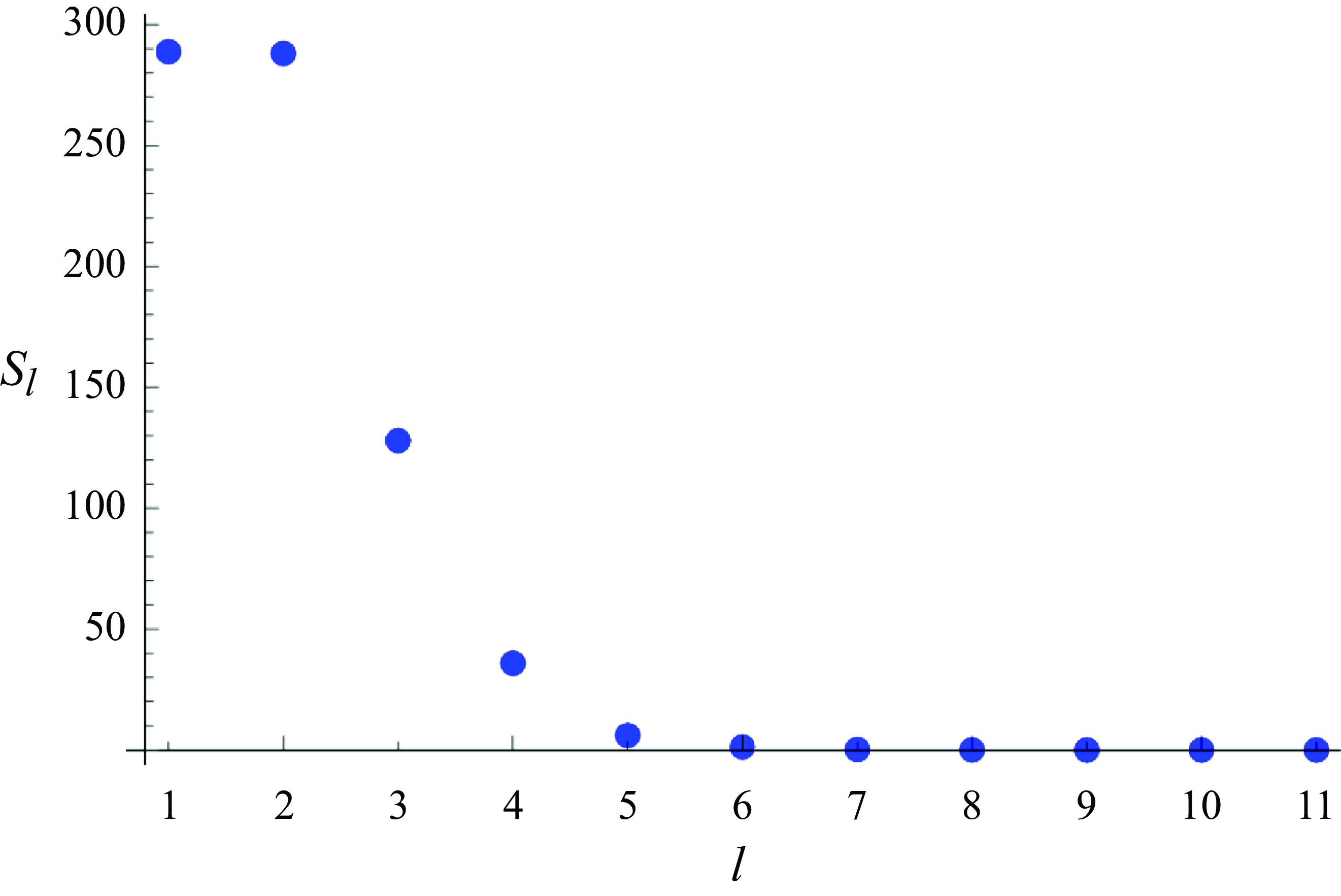
One comment on the numerical calculation of the stress should be made. As one can see, the upper limit of the sum in (2.112) is infinite. In the numerical calculation, we set a finite upper limit and increase it as long as the stress curve does not change any more. In figures 2(b,d,f,h), the stress curves do not change any more when the upper limit of the sum in (2.112) reaches 11, 10, 9 and 7, respectively. The process of the convergence of the stress curve to the final result can be characterised by the following quantity:

(3.1) \begin{equation} s_{l}=\sum _{k}\left[\sigma _{Lr\theta }^{\left(l\right)}\left(R_{20},\theta _{2k}\right)-\sigma _{Lr\theta }^{\left(\infty \right)}\left(R_{20},\theta _{2k}\right)\right]^{2} ,\end{equation}

where $0\leq \theta _{2k}\leq \pi , \sigma _{Lr\theta }^{(l)}(R_{20},\theta _{2k})$ is calculated by (2.112) setting the upper limit of the sum equal to l and $\sigma _{Lr\theta }^{(\infty )}(R_{20},\theta _{2k})$ is the value of the stress when the stress curve does not change any more. As an example, figure 3 shows $s_{l}$ for the stress curve presented in figure 2(b).

Figure 3.

Calculation of the convergence $s_{l}$ for the stress curve shown in figure 2(b).

Figure 4 illustrates cases where the particle material is different from steel. Figure 4(a) shows the acoustic streaming assuming that the particle material is copolymer with $\rho _{p}=900$ kg m⁻³, $E=1.1$ GPa, $\sigma =0.42 , \eta _{p}=0$ and $\zeta _{P}=0$ . Figure 4(b) shows the streaming assuming that the particle material is polystyrene with $\rho _{p}=1050$ kg m⁻³, $E=3.4$ GPa, $\sigma =0.34 , \eta _{p}=0$ and $\zeta _{P}=0$ . These materials are of interest because they are widely used in microfluidics (Nilsson et al. Reference Nilsson, Evander, Hammarström and Laurell2009; Leibacher, Hahn & Dual Reference Leibacher, Hahn and Dual2015). Figure 4(c) illustrates the case where the material parameters of the particle correspond to erythrocytes with $\rho _{p}=1125$ kg m⁻³, $E=26$ kPa, $\sigma =0.49 , \eta _{p}=0.006$ Pa s and $\zeta _{P}=0$ (Dulińska et al. Reference Dulińska, Targosz, Strojny, Lekka, Czuba, Balwierz and Szymoński2006). In all these cases, the bubble is assumed to undergo modes 0 and 1. For this excitation, the shear stress is shown in figure 2 to be the highest. The other parameters are as in figure 2. The stress curves for the above cases are shown in figure 4(d). They were obtained setting the upper limit of the sum in (2.112) equal to 9, 9 and 8, respectively. For comparison, the stress curve for the steel particle, shown in figure 2(f), is also included in figure 4(d).

Figure 4.

Acoustic streaming in the case that the particle material is (a) copolymer, (b) polystyrene and (c) the material parameters of the particle correspond to erythrocytes. The bubble undergoes modes 0 and 1. The other parameters are as in figure 2. (d) The stress curves for the cases shown in figures 4(a,c) and for the steel particle shown in figures 2(e,f).

For copolymer and polystyrene (materials with high rigidity), the overall streaming pattern is similar to that for the steel particle, shown in figure 2(e). The counter-rotating vortices are observed near the particle at $\theta _{2}=\pi$ and result in the rupture point on the particle’s surface at this location. The second possible rupture location is around the equator at $\theta _{2}=\pi /2$ , where another recirculation loop is clearly visible. A significant change occurs when a softer particle (erythrocyte) is considered. The direction of the streaming flow reverses around the location $\theta _{2}=0$ in comparison with the other stiff materials, and the recirculation vortices around the point facing the bubble almost disappear. In addition, while the distribution of the shear stress along the interface of the erythrocyte-like particle is similar to that for the stiffer particles, the stress magnitude for the erythrocyte-like particle is much smaller. Also, while the two poles of the particle are the places where rupture can occur in the case of a steel particle, softer materials (copolymer, polystyrene or erythrocyte) can only be ruptured near the equator or at the point facing the bubble. These findings differ from available results on bubble-induced mechanical effects (for instance, in the context of bubble-induced cell poration), where the cell is considered as an infinite elastic wall in front of which a single, infinitely small bubble is oscillating. For such a configuration, a single location of rupture is found at the point of the cell (wall) interface facing the bubble. When a finite-sized particle rather than an infinite wall is considered, the results of figures 2,4,5 display new findings, with the possibility of new points of rupture on the particle interface. When the bubble is experiencing the radial mode 0, the combination of radial and translational oscillations 0 –1 or the translational interaction 1–1 (figure 2 a,b,c) near a steel particle, the point of the particle interface facing the bubble is always the most probable location for rupture (with the highest stress and stress gradient magnitudes). For the same bubble driving, this behaviour does not change for stiff particles (copolymer and polystyrene, (figure 4 d)), but a change occurs for the erythrocyte-like particle. The shear stress gradient near the equator ( $\theta =\pi /2$ ) becomes similar in amplitude to that at the point facing the bubble ( $\theta =\pi$ ), so the equator becomes another location where rupture can be predominant.

Figure 5 illustrates the effect of the particle viscoelasticity. The parameters used, except the particle shear viscosity $\eta _{p}$ , are as in figure 4(c) for the erythrocyte-like particle. Figures 5(a,b) show acoustic streaming for $\eta _{p}=0.006$ Pa s and $\eta _{p}=0.06$ Pa s, respectively. Figure 5(c) shows the shear stress on the particle’s surface for increasing values of $\eta _{p}$ : 0.006 Pa s, 0.012 Pa s, 0.03 Pa s and 0.06 Pa s. As one can see, while the microstreaming pattern around the bubble remains almost unchanged whatever the particle shear viscosity (cf. figures 5 a,b), additional recirculation vortices appear near the particle for the higher shear viscosity. The distribution of the shear stress on the particle’s surface follows the same trend when $\eta _{p}$ increases (figure 5 c) but the maximal shear stress increases as the viscoelastic properties of the particle increase. Furthermore, the location of possible rupture at the particle equator and at the pole facing the bubble remains unchanged when the cell viscoelasticity is modified. The stress gradient at the point facing the bubble significantly increases, suggesting that high-viscosity particles may be more subjected to rupture under similar acoustic conditions.

Figure 6(b) shows a stress curve that was calculated for a radially oscillating bubble near a big particle at $R_{10}=5$ µm, $R_{20}=50$ µm, $d=65$ µm, $f=500$ kHz and $s_{0}=1$ −µm, the other parameters being as in figure 2. The curve does not change any more when the upper limit of the sum in (2.112) reaches 35. Figure 6(a) shows the system under consideration, keeping the real ratio of all sizes. Since $R_{10}\ll R_{20}$ , this case can be considered as an approximation of the behaviour of a bubble near a plane rigid wall. Note that, mathematically, ‘rigid wall’ means that Young’s modulus and the density of the wall tend to infinity. Numerical simulations do not allow infinite parameters. Therefore, for definiteness, we take the Young’s modulus and the density of steel. They are quite high, which allows one to consider that the behaviour of a steel wall is close to that of a rigid wall.

Figure 5.

The effect of the particle viscoelasticity. The parameters, except the particle shear viscosity $\eta _{p}$ , are as in figure 4(c). Panels (a) and (b) show acoustic streaming for $\eta _{p}=0.006$ Pa s and $\eta _{p}=0.06$ Pa s. Panel (c) shows the stress curves for increasing values of $\eta _{p}$ .

Figure 6.

(a) A radially oscillating bubble near a big particle.Here, $R_{10}=5$ µm, $R_{20}=50$ µm, $d=65$ µm, $f=500$ kHz, $s_{0}=1$ µm. (b) Shear stress produced by the bubble on the particle surface.

The time-averaged shear stress produced by an oscillating bubble on a plane rigid wall is commonly evaluated by using an approximation proposed by Nyborg (Reference Nyborg1958) for calculating acoustic streaming near a boundary. Based on this approximation, Doinikov & Bouakaz (Reference Doinikov and Bouakaz2014) have derived the following formula:

(3.2) \begin{equation} \sigma _{\tau }=\frac{\rho \delta }{8}\frac{\partial }{\partial \tau }\left(v_{\tau 0}v_{\tau 0}^{\ast }\right) ,\end{equation}

where $\sigma _{\tau }$ is the time-averaged shear stress produced by a radially oscillating bubble on a plane rigid wall, $\tau$ is the distance from the z axis along the wall and $v_{\tau 0}$ is the first-order velocity component directed along the wall (along $\tau$ ), which corresponds to the potential liquid flow and is taken at $z=d_{w}$ , where $d_{w}$ is the distance between the bubble centre and the wall; see figure 7(a). In the designations used in the present paper, $v_{\tau 0}$ is represented by

(3.3) \begin{equation} v_{\tau 0}=-e^{-i\omega t}\frac{2i\omega R_{10}^{2}s_{0}\tau }{\left(d_{w}^{2}+\tau ^{2}\right)^{3/2}}\left[1+\frac{R_{10}^{3}\chi }{d_{w}\left(d_{w}^{2}+\tau ^{2}\right)}\right] ,\end{equation}

where

(3.4) \begin{equation} \chi =\frac{3\left(x_{1}^{3}+3ix_{1}^{2}-6x_{1}-6i\right)}{4\left(18i+18x_{1}-3ix_{1}^{2}-x_{1}^{3}\right)} .\end{equation}

Figure 7.

(a) A radially oscillating bubble near a plane rigid wall. Here, $R_{10}=5$ µm, $d_{w}=15$ µm, $f=500$ kHz, $s_{0}=1$ µm. (b) Shear stress produced by the bubble on the wall, calculated by (3.5).

Substitution of (3.3) into (3.2) yields

(3.5) \begin{equation} \sigma _{\tau }=\frac{\omega ^{2}\rho \delta R_{10}^{4}|s_{0}|^{2}\tau }{\left(d_{w}^{2}+\tau ^{2}\right)^{4}}\left[d_{w}^{2}-2\tau ^{2}+\frac{2R_{10}^{3}\mathrm{Re}\left\{\chi \right\}\left(d_{w}^{2}-3\tau ^{2}\right)}{d_{w}\left(d_{w}^{2}+\tau ^{2}\right)}+\frac{R_{10}^{6}|\chi |^{2}\left(d_{w}^{2}-4\tau ^{2}\right)}{d_{w}^{2}\left(d_{w}^{2}+\tau ^{2}\right)^{2}}\right] .\end{equation}

For the same parameters as in figure 6, (3.5) gives the stress curve shown in figure 7(b). Comparing figures 6(b) and 7(b), one can see that the maximal stress magnitude predicted by our theory is 25.2 Pa, whereas (3.5) gives 1.1 Pa. This comparison suggests that the evaluation of the shear stress based on Nyborg’s approximation may considerably underestimate the stress magnitude.

In figures 6 and 7, the distance between the bubble’s surface and the particle’s surface (wall) is $2R_{10}=10$ µm. We have also made calculations for smaller distances between the bubble’s surface and the particle’s surface (wall): 5 µm and 1 µm. For these cases, the maximal stress magnitudes predicted by our theory are 155.4 Pa and 534.5 Pa, respectively, whereas (3.5) gives 7.4 Pa and 49.7 Pa, respectively. These results confirm that the calculation based on Nyborg’s approximation predicts a much lower stress than our model, which is based on a more rigourous calculation of acoustic streaming. It should be noted, however, that the difference between the results given by (3.5) and our model decreases with decreasing distance between the bubble and the particle.