2.1. General expressions

In this section, we recall general expressions for the magnetic field and plasma current in stellarators. Most of the results are well known and can be found in several places of the published literature, see e.g. the review by Helander (Reference Helander2014). The plasma is assumed to be in a scalar-pressure MHD equilibrium without flow, in which the magnetic-field lines trace out simply nested flux surfaces

(2.1) \begin{align} \boldsymbol {J} \times \boldsymbol {B} = \boldsymbol{\nabla }p, \end{align}

where $p$ denotes the pressure, $\boldsymbol {B}$ the magnetic field and $\boldsymbol {J}$ the current density. Boozer coordinates $(\psi ,\theta ,\varphi )$ can then be introduced and the magnetic field written as (Boozer Reference Boozer1981)

(2.2) \begin{align} \boldsymbol {B} = \boldsymbol{\nabla }\psi \times \boldsymbol{\nabla }\theta + \boldsymbol{\nabla }\varphi \times \boldsymbol{\nabla }\chi = G(\psi ) \boldsymbol{\nabla }\varphi + I(\psi ) \boldsymbol{\nabla }\theta + K(\psi ,\theta ,\varphi ) \boldsymbol{\nabla }\psi , \end{align}

where $\psi$ and $\chi$ measure toroidal and poloidal fluxes, respectively. The quantity $\psi$ is chosen to vanish on the magnetic axis, while $\chi$ is taken to vanish at the plasma edge and thus to attain its maximumFootnote ² on the magnetic axis. The function $I(\psi )$ is proportional to the total toroidal current enclosed by the flux surface $\psi$ . In most stellarators $I(\psi )$ is much smaller than $G(\psi )$ , since the current in the toroidal-field coils is much larger than the toroidal plasma current. The derivative $G'(\psi )$ is proportional to the pressure gradient, making $G(\psi )$ almost constant in a low-beta plasma. The Jacobian is

(2.3) \begin{align} \frac {1}{\sqrt {g}} = (\boldsymbol{\nabla }\psi \times \boldsymbol{\nabla }\theta ) \boldsymbol{\cdot }\boldsymbol{\nabla }\varphi = \frac {B^2}{G + \iota I}, \end{align}

where $\iota (\psi ) = {\rm d} \chi / {\rm d} \psi$ denotes the rotational transform. We shall also use another set of coordinates $(\psi ,\alpha ,l)$ , where $\alpha = \theta - \iota (\psi ) \varphi$ labels the different field lines on each flux surface, and $l$ denotes the arc length along each field line.

The flux-surface average of a function $f(\psi ,\theta ,\varphi )$ is defined as the volume average of this function over the region between two neighbouring magnetic surfaces

(2.4) \begin{align} \left \langle f \right \rangle = \frac {1}{V'(\psi )} \int _0^{2\pi } {\rm d} \theta \int _0^{2\pi /N_p} f(\psi ,\theta ,\varphi ) \sqrt {g(\psi ,\theta ,\varphi )} \; {\rm d} \varphi , \end{align}

where

(2.5) \begin{align} V'(\psi ) = \int _0^{2\pi } {\rm d} \theta \int _0^{2\pi /N_p} \sqrt {g} \; {\rm d} \varphi \end{align}

denotes the volume enclosed by the surface labelled by $\psi$ in one period of the stellarator, whose shape is assumed to be invariant under toroidal rotation by the angle $2 \pi / N_p$ . Here, $N_p$ denotes the number of field periods.

Since the divergence of the diamagnetic current

(2.6) \begin{align} \boldsymbol {J}_\perp = \frac {\boldsymbol {B} \times \boldsymbol{\nabla }p}{B^2} \end{align}

in general does not vanish, already Spitzer (Reference Spitzer1958) noted that there must be a current along $\boldsymbol {B}$ satisfying

(2.7) \begin{align} \boldsymbol {B} \boldsymbol{\cdot }\boldsymbol{\nabla }\left (\frac {J_\|}{B} \right ) = - (\boldsymbol {B} \times \boldsymbol{\nabla }p) \boldsymbol{\cdot }\boldsymbol{\nabla }\left ( \frac {1}{ B^{2}} \right ). \end{align}

The Pfirsch–Schlüter current is defined as the part of this current that does not contribute to the net toroidal current, i.e.

(2.8) \begin{align} J_{\|}^{\textrm {PS}} = J_{\|} - \frac {\left \langle J_{\|} B \right \rangle B}{\langle B^2 \rangle }. \end{align}

In the absence of an ohmic current, the bootstrap current and auxilliary current drive, $J_{\|}^{\textrm {PS}} = J_{\|}$ . As Boozer first observed, the Pfirsch–Schlüter current can be expressed in terms of the Fourier coefficients of

(2.9) \begin{align} \frac {1}{B^2} = \sum _{m,n} h_{mn}(\psi ) e^{i(m \theta - n \varphi )}, \end{align}

as

(2.10) \begin{align} \frac {J_\|^{\textrm {PS}}}{B} = -\frac {{\rm d}\kern-1pt p}{{\rm d} \psi } \sum _{m,n\ne 0} \frac {nI + mG}{m \iota - n} h_{mn} e^{i(m \theta - n \varphi )}, \end{align}

where each coefficient $h_{mn}(\psi )$ vanishes on the resonant surface where $\iota (\psi )=n/m$ . Otherwise, a current singularity arises, which has recently been analysed in detail by Huang et al. (Reference Huang, Zhou, Loizu, Hudson and Bhattacharjee2023).

2.2. Quasisymmetric magnetic fields

Quasisymmetric fields are those for which the field strength only depends on a linear combination of the Boozer angles, $B = B(\psi ,\theta - N \varphi )$ , where the integer $N$ vanishes in quasi-axisymmetric stellarators and usually coincides with the number of field periods in quasihelically symmetric ones. For such fields, any function of the form $f(\psi ,B)$ satisfies

(2.11) \begin{align} \boldsymbol {B} \boldsymbol{\cdot }\boldsymbol{\nabla }f & = \frac {\iota - N}{\sqrt {g}} \left ( \frac {\partial f}{\partial \theta } \right )_{\psi ,\varphi }\!,\\[-7pt]\nonumber \end{align}

(2.12) \begin{align} (\boldsymbol {B} \times \boldsymbol{\nabla }\psi ) \boldsymbol{\cdot }\boldsymbol{\nabla }f & = \frac {G + NI}{\sqrt {g}} \left ( \frac {\partial f}{\partial \theta } \right )_{\psi ,\varphi }\!, \end{align}

and (2.7) reduces to an ordinary differential equation that can be solved analytically, giving

(2.13) \begin{align} J_{\|}^{\textrm {PS}} = \frac {G + NI}{N-\iota } \frac {{\rm d}\kern-1pt p}{{\rm d} \psi } \left ( \frac {1}{B} - \frac {B}{\langle B^2 \rangle } \right )\!. \end{align}

Note that, in a tokamak or a quasi-axisymmetric stellarator ( $N = 0$ ), the Pfirsch–Schlüter current is proportional to $G/\iota$ , whereas in a quasihelically symmetric stellarator without net current ( $I = 0$ ), it is instead proportional to $G/(N - \iota )$ . It is thus relatively small if the number of field periods is large.

2.3. QI magnetic fields

By definition, a QI magnetic field satisfies the following two conditions (Helander & Nührenberg Reference Helander and Nührenberg2009; Nührenberg Reference Nührenberg2010).

1. (i) On each flux surface, all contours of constant field strength have the same topology and form poloidally closed curves, rather than toroidally or helically closed ones.

2. (ii) For trapped particles, the distance along the field between consecutive bounce points depends on the field strength at these points and on the flux surface on which they reside, but is the same for all field lines on that surface. In other words, in the coordinates $(\psi ,\alpha ,l)$ introduced above, the arc length between two points, $(\psi ,\alpha ,l_0)$ and $(\psi ,\alpha ,l_1)$ , of equal field strength on the same field line depends on $B(\psi ,\alpha ,l_0) = B(\psi ,\alpha ,l_1)$ and $\psi$ but not on the Clebsch angle $\alpha$ , provided that $B(\psi ,\alpha ,l) \lt B(\psi ,\alpha ,l_0)$ for all $l \in (l_0,l_1)$ . In particular, the distance between two consecutive field-strength maxima,

   (2.14) \begin{align} L(\psi ) = \int _{B(\psi ,\alpha ,l) \leqslant B_{\textrm {max}}(\psi )} {\rm d}l, \end{align}
   depends only on $\psi$ .

These conditions, which have been elaborated upon by Parra et al. (Reference Parra, Calvo, Helander and Landreman2015) and Helander et al. (Reference Helander, Goodman, Beidler, Kuczynski and Smith2024), guarantee that magnetically trapped particles, on a time average, drift in the poloidal direction rather than radially, toroidally or helically (Cary & Shasharina Reference Cary and Shasharina1997). They also ensure that, for any function $f\!(\psi ,B)$ ,

(2.15) \begin{align} \frac {\partial }{\partial \alpha } \int _{B(\psi ,\alpha ,l)\lt B} f[\psi ,B(\psi ,\alpha ,l)] {\rm d}l = 0. \end{align}

It was observed by Subbotin et al. (Reference Subbotin2006) that this property has an important implication for the Pfirsch–Schlüter current in the important case that the net toroidal current vanishes, $I(\psi ) = 0$ , so that $\boldsymbol {B} = G \boldsymbol{\nabla }\varphi + K \boldsymbol{\nabla }\psi$ . In the coordinate system $(\psi ,\alpha , l)$ , the equation for the Pfirsch–Schlüter current (2.7) then becomes

(2.16) \begin{align} \frac {\partial u}{\partial l} = - 2 \; \frac {\partial }{\partial \alpha } \left ( \frac {1}{B} \right ), \end{align}

where $u(\psi ,\alpha ,l) = J_\| / [p'(\psi ) B]$ . If we integrate this equation along the field over one period of the stellarator, from one field maximum to the next,Footnote ³ which we take to be located at $l=0$ and $l=L$ , respectively, and apply the Cary–Shasharina theorem (2.15), we obtain

(2.17) \begin{align} \frac {\partial }{\partial \alpha } \left [u(\psi ,\alpha ,L) - u(\psi ,\alpha ,0) \right ] = 0. \end{align}

If $I(\psi )=0$ , this condition not only implies that $ u(\psi ,\alpha ,L) - u(\psi ,\alpha ,0)$ is a constant independent of $\alpha$ , but also that $u(\psi ,\alpha ,0) = 0$ . This can be seen as follows. If we express $u$ in ordinary Boozer coordinates, $u = U(\psi ,\theta ,\varphi )$ , where $\varphi = 2 \pi n/N_p$ at the maxima of the field strength, then $U(\psi ,\theta ,0)$ must vanish for some $\theta$ , since the net toroidal current vanishes. Furthermore, the condition (2.17) and periodicity in $\varphi$ imply

(2.18) \begin{align} U(\psi ,\theta + 2 \pi \iota / N_p, 2 \pi / N_p) = U(\psi ,\theta + 2 \pi \iota / N_p, 0) = U(\psi ,\theta ,0). \end{align}

If the rotational transform $\iota$ is irrational, it follows that $U(\psi ,\theta ,0) = 0$ for all $\theta$ . In other words, the parallel current vanishes at the boundary of each field period, $\varphi = 2 \pi n/N_p$ , where the field strength reaches its maximum on each flux surface. The streamlines of $\boldsymbol {J}$ therefore cannot extend around the torus in the toroidal direction, but must ‘turn around’ in each period of the stellarator (Subbotin et al. Reference Subbotin2006; Helander Reference Helander2014).

Figure 1.

Value of $J_{\parallel}$ ( $\mathrm{A\,m^{-2}}$ ) on the $s=0.5$ flux surface of the ‘elongated QI’ configuration from Goodman et al. (Reference Goodman, Xanthopoulos, Plunk, Smith, Nührenberg, Beidler, Henneberg, Roberg-Clark, Drevlak and Helander2024), which has four field periods. Here, $s$ is the normalised toroidal flux, with $s=0$ on axis and $s=1$ on the boundary, and $(\theta ,\varphi )$ are the Boozer angles. The black curves show where $J_{\parallel}$ vanishes.

To give an example of what this looks like in a well-optimised QI field, we show a plot of $J_{\parallel}$ on a flux surface in the ‘elongated QI’ configuration from Goodman et al. (Reference Goodman, Xanthopoulos, Plunk, Smith, Nührenberg, Beidler, Henneberg, Roberg-Clark, Drevlak and Helander2024) in figure 1. This configuration, which has four field periods, was optimised for good QI quality at finite beta, and we use it without modification. As can be seen, $J_{\parallel}$ reaches the its highest magnitude approximately half-way through the period and its lowest magnitude close to $\varphi = 0$ and $\varphi = 2\pi /N_p = \pi /2$ . Note that the black curves, which mark where $J_\| = 0$ , stay close to these values of $\varphi$ , except for those two that separate the positive and negative regions of maximum magnitude. In a perfect QI field, the black curves would exactly coincide with the lines $\varphi = 0$ and $\varphi = 2\pi /N_p$ , but imperfections in the quasi-isodynamicity, which are inevitably present in any configuration, lead to the observed deviations.

3.1. Perturbed magnetic field

In order to investigate the Shafranov shift, we consider the effect of the addition of a small amount of plasma pressure to an otherwise zero-beta MHD equilibrium. For simplicity, we consider this question within the framework of reduced MHD (RMHD) (Strauss Reference Strauss1997; Zocco, Helander & Weitzner Reference Zocco, Helander and Weitzner2020) and assume that the net toroidal current vanishes. In other words, the magnetic field is written as $\boldsymbol {B} = \boldsymbol {B}_0 + \delta\kern-1pt \boldsymbol {B}$ , where the unperturbed equilibrium corresponds to $\beta =0$ and can thus be written as

(3.1) \begin{align} \boldsymbol {B}_0 = \boldsymbol{\nabla }\psi _0 \times \boldsymbol{\nabla }\theta + \boldsymbol{\nabla }\varphi \times \boldsymbol{\nabla }\chi _0 = G \boldsymbol{\nabla }\varphi , \end{align}

with constant $G$ . Here, and in the following, $(\psi ,\theta ,\varphi )$ denote Boozer coordinates associated with the unperturbed field, and for simplicity we have taken the net toroidal current to vanish.

The central assumption of RMHD is that there are two disparate scales on which the unperturbed and perturbed fields vary. The unperturbed magnetic field $\boldsymbol {B}_0$ is assumed to vary on a length scale $L_\|$ in all directions and the perturbation $\delta\kern-1pt \boldsymbol {B}_0$ is taken to vary on the much shorter scale $L_\perp$ in the directions perpendicular to $\boldsymbol {B}_0$ whereas it only varies on the longer scale $L_\|$ along $\boldsymbol { B}_0$ . In a stellarator, $L_\perp$ is thus identified with the minor radius $a$ and $L_\|$ with the major radius $R$ .Footnote ⁴ It follows that the gradients of the poloidal and toroidal angles scale as

(3.2) \begin{align} |\boldsymbol{\nabla }\theta | \sim \frac {1}{L_\perp }, \qquad |\boldsymbol{\nabla }\varphi | \sim \frac {1}{L_\|}, \end{align}

and the vectors $\boldsymbol{\nabla }\theta$ and $\boldsymbol{\nabla }\varphi$ are almost perpendicular since $\boldsymbol {B} = G \boldsymbol{\nabla }\varphi$ and

(3.3) \begin{align} \boldsymbol {B} \boldsymbol{\cdot }\boldsymbol{\nabla }\theta = \iota \boldsymbol {B} \boldsymbol{\cdot }\boldsymbol{\nabla }\varphi \sim \frac {B}{L_\|} \end{align}

imply $\boldsymbol{\nabla }\theta \boldsymbol{\cdot }\boldsymbol{\nabla }\varphi \sim \epsilon |\boldsymbol{\nabla }\theta ||\boldsymbol{\nabla }\varphi |$ , with $\epsilon = L_\perp / L_\| \ll 1$ . The rotational transform $\iota = {\rm d} \chi _0/{\rm d} \psi _0$ is treated as a number of order unity, and the poloidal and toroidal fluxes are thus comparable, $\psi _0 \sim \chi _0$ , although the poloidal field is much smaller than the toroidal one.

Turning to the MHD equations, we first note that the equilibrium condition

(3.4) \begin{align} \boldsymbol{\nabla }\left ( \mu _0 p + \frac {B^2}{2} \right ) - \boldsymbol {B} \boldsymbol{\cdot }\boldsymbol{\nabla }\kern-1.4pt\boldsymbol {B} = 0, \end{align}

becomes, to leading order in $\epsilon$ ,

(3.5) \begin{align} \boldsymbol{\nabla} _\perp (\boldsymbol {B}_0 \boldsymbol{\cdot }\delta\kern-1pt\boldsymbol {B} + \mu _0 p) = 0 \end{align}

and thus implies that $ \delta\kern-1pt \boldsymbol {B} = \delta\kern-1pt \boldsymbol {B}_\perp + \boldsymbol {b} \delta B_\|$ , with $\boldsymbol {b} = \boldsymbol {B}_0 / B_0$ and

(3.6) \begin{align} \frac {\delta B_\|}{B_0} = - \frac {\mu _0 p}{B_0^2} = - \frac {\beta }{2}. \end{align}

Furthermore, the relation $\boldsymbol{\nabla }\boldsymbol{\cdot }\delta\kern-1pt \boldsymbol {B}_\perp = - \boldsymbol{\nabla }\boldsymbol{\cdot }( \boldsymbol {b} \delta B_\|) \sim \epsilon \delta B_\perp / L_\perp$ implies that we can write

(3.7) \begin{align} \delta\kern-1pt \boldsymbol {B}_\perp = \boldsymbol{\nabla }\varphi \times \boldsymbol{\nabla }\delta \lambda + O(\epsilon ^2 B_0) \end{align}

for some function $\delta \lambda (\psi ,\theta ,\varphi ) \ll \chi _0$ . (All perturbations are marked with a $\delta$ .) This streamfunction of the perpendicular field can be related to the poloidal- and toroidal-flux perturbations by noting that $ \delta\kern-1pt \boldsymbol {B}$ can also be written as

(3.8) \begin{align} \delta\kern-1pt \boldsymbol {B} = \boldsymbol{\nabla }\delta \psi \times \boldsymbol{\nabla }\theta + \boldsymbol{\nabla }\varphi \times \boldsymbol{\nabla }\delta \chi + \boldsymbol{\nabla }\psi \times \boldsymbol{\nabla }\delta k \end{align}

for some functions $\delta \psi$ , $\delta \chi$ and $\delta k$ .Footnote ⁵ Hence it follows that, to leading order,

(3.9) \begin{align} \delta\kern-1pt \boldsymbol {B}_\perp \times \boldsymbol{\nabla }\varphi = |\boldsymbol{\nabla }\varphi |^2 \boldsymbol{\nabla }\delta \chi - (\boldsymbol{\nabla }\theta \boldsymbol{\cdot }\boldsymbol{\nabla }\varphi ) \boldsymbol{\nabla }\delta \psi = |\boldsymbol{\nabla }\varphi |^2 \left ( \boldsymbol{\nabla }\delta \chi - \iota \boldsymbol{\nabla }\delta \psi \right ), \end{align}

where we have used the fact that, for any perturbation $\delta f$ , the derivative along $\boldsymbol {B}_0$ is relatively small

(3.10) \begin{align} \boldsymbol {B}_0 \boldsymbol{\cdot }\boldsymbol{\nabla }\delta f \ll B_0 |\boldsymbol{\nabla }\delta f |. \end{align}

According to (3.6), the toroidal-flux perturbation is of order $\delta \psi = O(\beta \psi )$ , but the perturbation in poloidal flux is much larger, $\delta \chi = O(\delta \psi / \epsilon )$ , since the poloidal- and toroidal-field perturbations are comparable, $\delta B_\perp \sim \delta B_\|$ . It follows that the last term in (3.9) is relatively small, and from (3.7) and (3.9) we thus conclude that $\delta \lambda$ is approximately equal to the poloidal-flux perturbation, $\delta \lambda \simeq \delta \chi$ .

In conclusion, then, the addition of a small amount of pressure, $\beta \ll \epsilon$ , to a vacuum field (3.1) causes the poloidal flux to change from $\chi _0$ to $\chi = \chi _0 + \delta \chi$ , where $\delta \chi /\chi _0 = O(\beta /\epsilon )$ . This perturbation leads to a slight movement of the plasma column, which will be quantified in the next subsection by making use of the fact that the parallel current is related to $\delta \chi$ by

(3.11) \begin{align} \mu _0 J_\| = \boldsymbol {b} \boldsymbol{\cdot }( \boldsymbol{\nabla }\times \delta\kern-1pt \boldsymbol {B}_\perp ) \simeq \frac {B}{G} \boldsymbol{\nabla} ^2 \delta \chi , \end{align}

to leading order in $\epsilon$ .

3.2. Average Shafranov shift

The movement and the deformation of the flux surfaces constitute the Shafranov shift, which depends both on the pressure-induced currents inside the plasma and on the boundary condition at the plasma edge. The Shafranov shift is therefore different in fixed-boundary and free-boundary equilibria. In the former, the fixed boundary remains a flux surface as pressure is added whereas in free-boundary equilibria the plasma boundary will in general be deformed. We focus on the former case, where $\chi =0$ on the fixed boundary.

Figure 2.

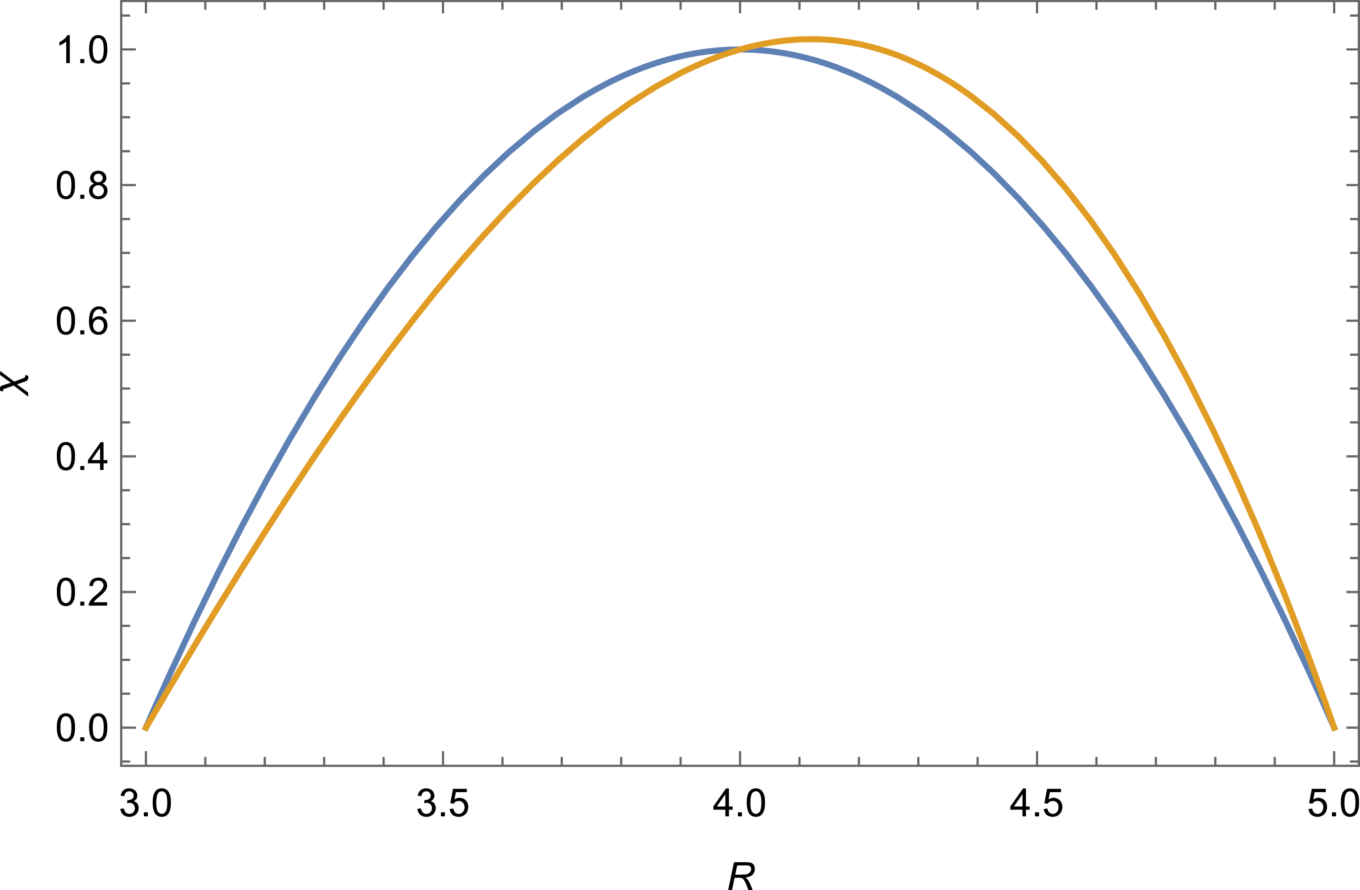
Schematic figure illustrating how the poloidal flux $\chi$ may vary along a long a ray (here in terms of the major radius $R$ ) in a fixed-boundary equilibrium without (blue) and with (orange) plasma pressure. The poloidal flux vanishes at the boundary and peaks on the magnetic axis. With increasing pressure, the magnetic axis moves outward, and the spatial distribution of $\chi$ changes accordingly.

In order to quantify the average Shafranov shift, we introduce the functional

(3.12) \begin{align} S[\chi ] & = \frac {1}{X} \int _P \chi F {\rm d}V ,\\[-7pt]\nonumber \end{align}

(3.13) \begin{align} X & = \int _P \chi {\rm d}V, \end{align}

where $F(\boldsymbol {r})$ is a suitably chosen function of the coordinates $\boldsymbol {r}$ and the integral is taken over the plasma volume $P$ . Here, $S[\chi ]$ can be regarded as a $\chi$ -weighted average of the function $F(\boldsymbol {r})$ over the domain $P$ . The Shafranov shift is the amount by which $S[\chi ]$ changes due to the redistribution of poloidal flux when pressure is added, see figure 2. To first order in $\delta \chi /\chi _0 \ll 1$ , we have

(3.14) \begin{align} \delta S = S[\chi _0 + \delta \chi ] - S[\chi _0] = \frac {1}{X} \left ( \int _P \delta \chi F {\rm d}V - S[\chi _0] \int _P \delta \chi {\rm d}V \right ), \end{align}

where the second term in the brackets vanishes if either $F(\boldsymbol {r})$ is chosen so that $S[\chi _0] = 0$ or the volume integral of $\delta \chi$ vanishes.Footnote ⁶ In the following, we shall assume this to be the case.

Different choices of $F$ correspond to different manifestations of the Shafranov shift. For instance, choosing $F = \delta (\boldsymbol {r} - \boldsymbol {r}_0)$ is synonymous with declaring an interest in the value of the poloidal flux in the point $\boldsymbol {r}_0$ . If this point lies on the magnetic axis of the vacuum field, then $\delta S$ measures how far the magnetic axis moves away from that point, due to the addition of pressure, in terms of poloidal flux. (If $F$ is chosen in this way, then $S[\chi _0] \ne 0$ and we must instead require that the volume integral of $\delta \chi$ vanishes.) Another choice of interest is

(3.15) \begin{align} F(\boldsymbol {r}) = x(\boldsymbol {r}), \end{align}

where $x$ is a coordinate in the plane perpendicular to $\boldsymbol {B}_0$ that increases in a direction that is deemed interesting. Then, $S[\chi ]$ measures a $\chi$ -weighted average of $x$ over the domain, and $\delta S$ indicates how far the poloidal flux has moved, on average, in the $x$ -direction. Whatever the exact definition of $F$ , we shall normalise it in such a way that a Shafranov shift of order unity, $\delta S = O(1)$ , corresponds to a displacement of the plasma column comparable to the minor radius $a$ .

In order to derive a useful expression for $\delta S$ , we introduce a function $H(\boldsymbol {r})$ such that

(3.16) \begin{align} {\nabla} ^2 H = F \end{align}

everywhere in the plasma volume $P$ and $H=0$ on the boundary. These conditions uniquely determine $H$ , which encapsulates the necessary information about the shape of the plasma cross-section and is discussed in Appendix A. Our measure of the Shafranov shift can now be written as

(3.17) \begin{align} X \delta S = \int _P \delta \chi {\nabla} ^2 H {\rm d}V = \int _P H {\nabla} ^2 \delta \chi \; {\rm d}V = \mu _0 G \int _P \frac {H J_\|}{B} \; {\rm d}V, \end{align}

where we have used (3.11) and the fact $\delta \chi$ vanishes on the boundary. Note that, in RMHD, the Shafranov shift is exclusively caused by the parallel (Pfirsch–Schlüter) current to leading order in $\epsilon$ . It is assumed that the net toroidal current vanishes, on each flux surface, both before and after the addition of pressure. The case of a ‘flux-conserving stellarator’ (Freidberg Reference Freidberg2014) is thus not considered.

A general, yet explicit, expression for the Shafranov shift in a stellarator without net toroidal current can be obtained by substituting (2.10) in (3.17),

(3.18) \begin{align} \delta S = \frac {\mu _0 G^2}{X} \sum _{m,n\ne 0} \int _P \frac {{\rm d}\kern-1pt p}{{\rm d} \psi } \frac {h_{mn} H}{\iota - n/m} e^{i(m \theta - n \varphi )} \; {\rm d}V, \end{align}

where all necessary information about the magnetic-field geometry is encapsulated in the quantities $X$ , $h_{mn}$ and $H$ .

An equally general upper bound on $\delta S$ follows from (3.17) and the Cauchy–Schwarz inequality

(3.19) \begin{align} \delta S \leqslant \frac {\mu _0 G}{X} \left [ \int _P H^2 {\rm d}V \int _P \left ( \frac {J_\|}{B} \right )^2 {\rm d}V \right ]^{1/2}, \end{align}

where $J_\|$ is related to the pressure by (2.7). It is clear from (3.17) and (3.19) that the Shafranov shift is particularly small in a magnetic field optimised for small Pfirsch–Schlüter current (Wobig Reference Wobig1999).

Before closing this section, we note that there is no way of avoiding the Shafranov shift altogether by optimising the magnetic-field geometry. The average Shafranov shift (3.17) does not vanish for all allowable functions $H$ unless the Pfirsch–Schlüter current $J_\|$ vanishes everywhere. This happens only if the field lines are geodesics, i.e. if the magnetic field is isodynamic, which is impossible in practice (Helander Reference Helander2014). In the context of axisymmetric fields, Bishop & Taylor (Reference Bishop and Taylor1986) considered the related question (without the RMHD approximation) by asking whether the Grad–Shafranov equation has solutions with identically shaped flux surfaces but different pressure and current profiles.

4.1. General geometry

In Boozer coordinates, (2.7) becomes

(4.1) \begin{align} \frac {\partial u}{\partial \varphi } + \iota \frac {\partial u}{\partial \theta } = - G \frac {\partial\kern-1pt B^{-2}}{\partial \theta } = f(\theta ,\varphi ), \end{align}

where again $u = J_\| / (Bp'(\psi ))$ , and since $\partial\kern-1pt B/\partial \theta = O(\epsilon )$ in the RMHD ordering, it follows that $ u \sim G \epsilon / B^2$ . This general scaling shows how $u$ depends on $\epsilon$ when $\iota$ is order unity, but it is modified if $\iota \gg 1$ , in which case an additional factor $\iota$ appears in the denominator

(4.2) \begin{align} u \sim \frac {G \epsilon }{\iota B^2}. \end{align}

This is perhaps obvious already from (4.1) but can also be verified by inspecting the solution

(4.3) \begin{align} u(\theta ,\varphi ) = \int _{\varphi _0}^\varphi f\left [ \theta + \iota ( \varphi ' - \varphi ), \varphi ' \right ] {\rm d} \varphi ', \end{align}

where $\varphi _0(\theta ,\varphi )$ is chosen so that $u[\theta + \iota ( \varphi _0 - \varphi ),\varphi _0] = 0$ . In the limit $\iota \gg 1$ , the integrand $g(\varphi ') = f[ \theta + \iota ( \varphi ' - \varphi ), \varphi ' ]$ becomes almost periodic with a period of $2 \pi / \iota$ since

(4.4) \begin{align} g(\varphi ' + 2\pi / \iota ) - g(\varphi ') = O( \iota ^{-1}). \end{align}

More importantly, its integral over one period is of order

(4.5) \begin{align} \int _{\varphi _0 + 2 \pi n/\iota }^{\varphi _0 + 2 \pi (n+1)/\iota } g(\varphi ') {\rm d} \varphi ' = O(\iota ^{-2}), \end{align}

since, by the definition of $f(\theta ,\varphi )$ ,

(4.6) \begin{align} \int _0^{2\pi } f(\theta , \varphi ) {\rm d} \theta = 0. \end{align}

Hence, we conclude that $u \sim f/\iota$ , and (4.2) follows if $\iota$ is either comparable to, or larger than, unity. If we further estimate, within factors of order unity, $G \sim BR$ , $\chi \sim \iota \psi \sim \iota B a^2$ , we arrive at a universal scaling of the average Shafranov shift (3.17)

(4.7) \begin{align} \delta S \sim \frac {\beta }{\epsilon \iota ^2}. \end{align}

The equilibrium pressure limit is thus expected to scale as (1.1), indicating that Spitzer’s result is of general validity to the present level of accuracy. As long as the magnetic field follows the RMHD ordering, this is how the equilibrium beta limit scales with $\epsilon$ and (more approximately) with $\iota$ .

Slightly more precise results can be derived for quasisymmetric and QI stellarators, to which we now turn our attention.

4.2. Quasisymmetric stellarators

In a quasisymmetric stellarator without net toroidal current, $I=0$ , (2.13) and (3.17) give the following explicit formula for $\delta S$ :

(4.8) \begin{align} \delta S_{\textrm {QS}} = \frac {\mu _0 G^2}{X} \int _P \frac {p'(\psi )}{N-\iota } \left \langle H \left ( \frac {1}{B^2} - \frac {1}{\langle B^2 \rangle } \right ) \right \rangle {\rm d}V. \end{align}

According to the ordering underlying RMHD, the magnetic-field strength $B$ only varies on the long length scale $L_\|$ , which is taken to be comparable to the circumference of the torus. In a quasi-axisymmetric (QA) or quasihelically (QH) symmetric stellarator, $B$ is constant along the magnetic axis and can therefore only vary by a relative amount of order $\epsilon = L_\perp /L_\| \ll 1$ in the entire plasma volume. Again using $G \sim BR$ and $\chi \sim \iota B a^2$ gives

(4.9) \begin{align} \frac {J_{\|}^{\textrm {PS}}}{B} = \frac {G}{N-\iota } \frac {{\rm d}\kern-1pt p}{{\rm d} \psi } \left ( \frac {1}{B^2} - \frac {1}{\langle B^2 \rangle } \right ) \sim \frac {R\kern-1pt B}{N - \iota } \frac {p}{a^2B} \frac {\epsilon }{B^2} = \frac {p}{(N-\iota ) a\kern-1.3pt B^2}, \end{align}

within factors of order unity. It follows that the Shafranov shift (4.8) in a quasisymmetric stellarator is of order

(4.10) \begin{align} \delta S_{\textrm {QS}} \sim \frac {\beta }{|N-\iota |\iota \epsilon }, \end{align}

where we have again crudely estimated the poloidal flux by $\chi \sim \iota \psi$ . The equilibrium pressure limit is thus expected to scale as

(4.11) \begin{align} \beta _{\textrm {QS}} \sim \left | \frac {N}{\iota } - 1 \right | \epsilon \iota ^2. \end{align}

These scalings agree with the classical-stellarator result (1.1) but contain an additional dependence on $N / \iota$ .

4.3. QI stellarators

In a QI stellarator, the Shafranov shift must of course follow the approximate general scaling (4.7), but it is also possible to derive a quantitatively precise result. As we have already seen, the Pfirsch–Schlüter current in a QI stellarator without net toroidal current satisfies (2.16), but unlike the quasisymmetric case, there is no closed form for the solution of this equation. It is, however, possible to use (3.19) to derive an upper bound on the Shafranov shift. We start by noting that

(4.12) \begin{align} \langle u^2 \rangle = \frac {1}{V'(\psi )} \oint {\rm d} \alpha \int _0^Y u^2 {\rm d}y, \end{align}

where ${\rm d}y = {\rm d}l/B$ and the integral

(4.13) \begin{align} Y(\psi ) = \int _0^L \frac {{\rm d}l}{B}, \end{align}

is performed along $\boldsymbol {B}$ over one period of the device, $\varphi \in [0,2\pi /N_p]$ . By using the Poincaré inequality

(4.14) \begin{align} \int _0^Y u^2 {\rm d}y \leqslant \left ( \frac {Y}{\pi } \right )^2 \int _0^Y \left ( \frac {\partial u}{\partial y} \right )^2 {\rm d}y, \end{align}

for functions such that $u(0) = u(Y) = 0$ , we conclude from (2.16) that

(4.15) \begin{align} \langle u^2 \rangle \leqslant \frac {4Y^2}{\pi ^2 V'} \oint {\rm d} \alpha \int _0^L \left ( \frac {\partial \ln B}{\partial \alpha } \right )^2 \frac {{\rm d}l}{B}. \end{align}

Since $V'(\psi ) = 2 \pi Y(\psi )$ , this result can be written as

(4.16) \begin{align} \left \langle \left ( \frac {J_\|}{B} \right )^2 \right \rangle \leqslant \frac {1}{\pi ^4} \left \langle \left ( p' V' \frac {\partial \ln B}{\partial \alpha } \right )^2 \right \rangle , \end{align}

which can be substituted into (3.19) to give an upper bound on the Shafranov shift in QI stellarators without net toroidal current

(4.17) \begin{align} \delta S_{\textrm {QI}} \leqslant \frac {\mu _0 G}{\pi ^2 X} \left [ \int _P H^2 {\rm d}V \int _P \left (p' V' \frac {\partial \ln B}{\partial \alpha } \right )^2 {\rm d}V \right ]^{1/2}. \end{align}

Ignoring factors of order unity in the estimates $ V'(\psi ) \sim {2 \pi R}/({N_pB})$ , $p'(\psi ) \sim p/(a^2 B)$ and

(4.18) \begin{align} \frac {\partial \ln B}{\partial \alpha } \sim \epsilon , \end{align}

gives the scaling

(4.19) \begin{align} \delta S_{\textrm {QI}} \:{\stackrel {\textstyle {\lt }}{\sim }}\: \frac {\beta }{N_p\iota \epsilon }, \end{align}

thus suggesting a beta limit

(4.20) \begin{align} \beta _{\textrm {QI}} \sim \frac {N_p}{\iota } \epsilon \iota ^2. \end{align}

Apart from the dependence on $N_p/\iota$ , this scaling agrees with that for classical stellarators (1.1) and quasisymmetric ones (4.10). It should be noted that, in many cases, (4.18) is likely to be an overestimate of the poloidal magnetic-field-strength variation since the field strength may vary by less than $O(\epsilon )$ in the poloidal direction of a QI stellarator. This variation vanishes identically on the contour $B = B_{\textrm {max}}(\psi )$ and can be made quite small elsewhere by targetted optimisation of the magnetic-field geometry, which then results in a correspondingly smaller Shafranov shift.