2. Main results and discussion

Recall that throughout we assume that X satisfies the conditions in (1.4) and that (1.5) holds. In the first lemma we show, using standard arguments, that the optimal prediction problem (1.1) can be expressed as an optimal stopping problem driven by the process $Y^0$.

Lemma 2.1. Let the non-negative function H be given by

(2.1) \begin{equation}H(y) = \varphi(y) \left( 1-e^{-\Phi y} \right) + \int_y^\infty \varphi(z)\Phi e^{-\Phi z} \, \textrm{d} z \quad \text{for all $y \geq 0$},\end{equation}

and further define the function V as

(2.2) \begin{equation}V(y) = \inf_\tau {\mathbb{E}}[H(Y^y_\tau)] \quad \text{for all $y \geq 0$},\end{equation}

where the infimum is taken over all stopping times with respect to the naturally enlarged filtration generated by $Y^y$.

Then V(0) equals (1.1).

Proof. Since $\varphi$ is non-negative, we can assume in the below without loss of generality that $\varphi$ is bounded (the result can be extended using monotone convergence otherwise). We closely follow the proof of Lemma 1 in [Reference Du Toit and Peskir11], first establishing for any $t \geq 0$ that

\[ {\mathbb{E}} \left[ \left. \varphi \left( \overline{X}_\infty-X_t \right) \, \right| \, \mathcal{F}_t \right] = {\mathbb{E}} \left[ \varphi \left( y+ (\overline{X}_\infty-y)^+ \right) \right] \Big|_{y=\overline{X}_t-X_t}. \]

Using that $\overline{X}_\infty \sim \text{Exp}(\Phi)$ (cf. (1.4)), a straightforward computation shows that the right-hand side of the above equals $H(\overline{X}_t-X_t)$. An application of Hunt’s lemma (cf. e.g. E14.1 in [Reference Williams24]) now yields the result. □

Note that for $y>0$, we can understand V(y) to be equivalent to (1.1) in the situation that X was started at some time prior to $t=0$ and at $t=0$ we observe the reflected distance to be $y=\overline{X}_0-X_0$.

It is not hard to show that if the penalty function $\varphi$ is non-decreasing then for $y=0$ it is optimal to stop immediately. Apparently the homogeneity of X, together with the fact that X drifts to $-\infty$, guarantees that waiting is suboptimal and that (1.1) is equal to ${\mathbb{E}}[\varphi (\overline{X}_\infty)]$.

Proof. By virtue of Lemma 2.1 above, since $Y^0_0=0$ it suffices to show that H is non-decreasing. For this, take any $0 \leq y_1 \leq y_2$ and note that integration by parts yields

\[ \int_{y_1}^{y_2} \varphi(z) \Phi e^{-\Phi z} \, \textrm{d} z = -\varphi(y_2) e^{-\Phi y_2}+\varphi(y_1) e^{-\Phi y_1} + \int_{y_1}^{y_2} e^{-\Phi z} \textrm{d}\varphi(z), \]

so that

\[ H(y_2)-H(y_1) = \varphi(y_2) - \varphi(y_1) - \int_{y_1}^{y_2} e^{-\Phi z} \textrm{d}\varphi(z). \]

Since $\varphi$ is non-decreasing we have that

\[ \int_{y_1}^{y_2} e^{-\Phi z} \textrm{d}\varphi(z) \leq \int_{y_1}^{y_2} \textrm{d}\varphi(z) = \varphi(y_2) - \varphi(y_1) \]

and hence indeed $H(y_2)-H(y_1) \geq 0$. □

Now we turn to the more interesting case of a quadratic penalty function of the form

(2.3) \begin{equation}\varphi(x) =(x-b)^2 \quad \text{for some $b > 0$,}\end{equation}

in which case H as defined in (2.1) boils down to

(2.4) \begin{equation}H(y) = (y-b)^2+\frac{2}{\Phi} e^{-\Phi y} \left( y-b + \frac{1}{\Phi} \right).\end{equation}

Note that the shape of $\varphi$ is preserved in H in the sense that H′ is $<0$, $=0$, $>0$ for $y \in (0,b)$, $y=b$, $y>b$ respectively, with $H(0)<\infty$ and $H(\infty)=\infty$. Hence it makes sense to expect that in the optimal stopping problem (2.2) it is optimal to stop when $Y^y$ is close to b, i.e. when the distance between the running supremum and the position of X is close to b.

However, keeping in mind that $Y^y$ drifts to $\infty$, for any $y \in (b,\infty)$ it is not obvious whether it is better to stop and accept the payoff $H(y)>H(b)$ or to wait until $Y^y$ moves closer to b while risking that it will only drift farther away from b. Furthermore, for any $y \in [0,b)$ there is a similar dilemma, where waiting for $Y^y$ to move closer to b comes with the risk of a positive jump taking $Y^y$ (far) over the level b to more unfavourable payoffs. So the structure of the solution is not very easy to guess.

Before presenting our main result we make two assumptions in addition to the conditions in (1.4):

1. (A1) There exists $z_0<0$ such that $\psi(z_0)<\infty$.

2. (A2) If X has bounded variation then $\Pi$ has no atoms.

Recall that (A1) is a restriction on the ‘large jumps’, in the sense that it is equivalent to

\[ \int_{(-\infty,-1)} e^{z_0 x} \Pi(\textrm{d}x)<\infty \]

(cf. Theorem 3.8 in [Reference Kyprianou18]). It guarantees that the domain of $\psi$ (on the interior of which it is infinitely-often differentiable and strictly convex) contains $[z_0,\infty)$. In particular it implies that all the integer moments of $X_1$ are finite, and $\psi^{(k)}(0)$ equals the kth cumulant of $X_1$. The assumption (A2) is needed to exclude some pathological cases in the proofs.

Further recall that there exist families of scale functions associated with X, denoted by $W^{(q)}\,:\, {\mathbb{R}} \to [0,\infty)$ and $Z^{(q)}\,:\, {\mathbb{R}} \to [1,\infty)$ for $q \geq 0$, where $W^{(q)}(x)=0$ for $x<0$, while on $[0,\infty)$ $W^{(q)}$ is continuous, strictly increasing, and uniquely characterised by

\[ \int_0^\infty e^{-\beta x} W^{(q)}(x) \, \textrm{d} x = \frac{1}{\psi(\beta)-q} \quad \text{for $\beta>\Phi(q)$,} \]

and where

\[ Z^{(q)}(x) = 1+q \int_0^x W^{(q)}(y) \, \textrm{d} y \quad \text{for $x \in {\mathbb{R}}$.} \]

For simplicity we define $W:\!=W^{(0)}$ and $Z:\!=Z^{(0)}$. These scale functions are commonly used to express quantities involving one- and two-sided exit problems for X; see e.g. Chapter 8 in [Reference Kyprianou18]. Explicit expressions (or numerical algorithms) exist for many cases; cf. e.g. [Reference Hubalek and Kyprianou15] (see also Section 4 below).

Here is our main result, which fully characterises the solution to the optimal stopping problem (2.2).

Theorem 2.1. Consider the optimal stopping problem (2.2) for H given by (2.4). Suppose that the assumptions (A1) and (A2) above hold in addition to the conditions in (1.4). Furthermore, we define for $y \geq 0$ and $a \geq 0$ the stopping time

\[ \tau^y_a = \inf \{ t \geq 0 \, | \, Y^y_t \geq a \}, \]

and we set

\[ I_1(a)=\int_0^a W(x) \, \textrm{d} x, \quad I_2(a)=\int_0^a xW(x) \, \textrm{d} x, \quad \text{and} \quad I_3(a)=\int_0^a e^{-\Phi x} W(x) \, \textrm{d} x. \]

We have the following two cases:

1. (i) If

   \[ b \leq \frac{\psi'(\Phi)/\Phi-\psi''(0)/2}{\psi'(0)} \]
   then for any $y \geq 0$ it holds that $\tau=0$ is optimal in (2.2) and hence $V=H$.

2. (ii) If

   \[ b > \frac{\psi'(\Phi)/\Phi-\psi''(0)/2}{\psi'(0)} \]
   then there exists $a^* \in (0,b]$ such that for any $y \geq 0$ the stopping time $\tau^y_{a^*}$ is optimal in (2.2). A characterisation of $a^*$ is given in Lemma 3.3. Furthermore, V is continuous and can be expressed as
   \[ V(y) = \begin{cases}H(y) - I_1(a^*-y) \big( 2\psi'(0)(b-y)+\psi''(0) \big) & \\ \qquad +2\psi'(0)I_2(a^*-y)+2\psi'(\Phi)e^{-\Phi y} I_3(a^*-y)/\Phi & \text{if $y \in [0,a^*)$,} \\[5pt] H(y) & \text{if $y \in [a^*,\infty)$.}\end{cases} \]

A proof is provided in Section 3. Case (i) is covered by Lemmas 3.4 and 3.10, while for Case (ii) Lemmas 3.4 and 3.9 give the optimal stopping time, and the expression for V follows from Lemma 3.2.

This result shows that in both Case (i) and Case (ii), if the process $Y^y$ starts in $(b,\infty)$ (i.e. $y \in (b,\infty)$), then it is best to stop immediately. That is to say, it is not worth waiting for $Y^y$ to decrease closer to b, because of the risk that it will move upwards instead. Furthermore, in Case (ii), if the process $Y^y$ starts in $(0,a^*)$, then it is optimal to wait until $Y^y$ gets closer to b and to stop only when it first enters $[a^*,\infty)$. Note that it is indeed very well possible that $a^*<b$ (see also Section 4); in this situation it is optimal to stop when $Y^y$ is close enough to b, rather than waiting until $Y^y$ actually hits the level b and risking that a positive jump takes $Y^y$ (deep) into $(b,\infty)$.

The distinction between the two cases in the result is also interesting. It can be verified that

(2.5) \begin{equation}\frac{\psi'(\Phi)/\Phi-\psi''(0)/2}{\psi'(0)}\end{equation}

is non-negative, and that it vanishes if and only if X has no jumps, i.e. when X is a Brownian motion with negative drift (cf. Lemma 3.1). Indeed, if X has no jumps then neither has $Y^y$, and therefore it is obvious that while $Y^y$ lives in [0,b) it is best to wait for it to hit b (which it will a.s.). The above result confirms this since Case (ii) always applies in this situation (with $a^*=b$). On the other hand, if X does have jumps then b has to be large enough (or, the difference between H(y) for y close to 0 and H(b) has to be large enough) for the benefit of waiting for $Y^y$ to get closer to b to outweigh the risk of a jump taking $Y^y$ (far) beyond b.

Finally it is worth noting that we would expect the above result to remain valid under the weaker condition that only the first moment of $X_1$ is guaranteed to be finite. It would then seem that the same two cases remain present as long as the second moment is also finite, but that when the second moment is infinite, (2.5) is also infinite since $\psi'(0)\lt 0$ and $\psi''(0)={\textrm{var}}(X_1)=\infty$, so that only the first case is present. This is of course due to the quadratic form of the penalty function.

3. Remaining proofs

This section contains a proof of Theorem 2.1, broken down into a number of lemmas. We use the notation introduced above and in the statement of Theorem 2.1 throughout.

The proof is a bit hairy since the optimal stopping problem (2.2) involves a payoff function H that is not monotone or convex/concave (often for payoff functions with such properties more straightforward arguments are possible), and furthermore, since $H(Y^y_t) \to \infty$ a.s. as $t \to \infty$, the integrability conditions that are typically assumed when formulating general results in optimal stopping theory do not hold in this case.

Recall that we are working under the assumption that the conditions in (1.4) hold, and that (A1) and (A2) from Section 2 hold. Using (A1), in the interior of the domain of $\psi$, which contains the point 0, we get from (1.3) that

(3.1) \begin{align} \psi'(z) & \,=\,\sigma^2 z-\gamma+\int_{(-\infty,0)} \left( xe^{zx}-x\mathbf{1}_{\{ x>-1 \}} \right) \Pi(\textrm{d}x),\nonumber\\[3pt] \psi''(z) & \,=\,\sigma^2+\int_{(-\infty,0)} x^2 e^{zx} \Pi(\textrm{d}x) \quad \text{and} \quad \psi'''(z)=\int_{(-\infty,0)} x^3 e^{zx} \Pi(\textrm{d}x). \end{align}

Briefly returning to the scale functions introduced in Section 2, from Lemma 8.6 in [Reference Kyprianou18] we know that $W(0)=0$ if X has unbounded variation and $W(0)>0$ otherwise. Furthermore, using (A2) we know that $W \in C^1(0,\infty)$ and $W'>0$ on $(0,\infty)$, and the right derivative at 0 exists; with a slight abuse of notation we denote the latter by $W'(0) \in (0,\infty]$ (cf. Lemma 8.2 and the discussion following it, and Exercise 8.5, both in [Reference Kyprianou18]).

Furthermore, for twice continuously differentiable functions $f\,:\,{\mathbb{R}}\to{\mathbb{R}}$ we define

(3.2) \begin{equation}\mathcal{A}f(y) = \frac{\sigma^2}{2} f''(y)+\gamma f'(y) + \int_{{\mathbb{R}}} \big( f(y+x)-f(y)+x f'(y) \mathbf{1}_{\{ |x|<1 \}} \big) \Pi(\textrm{d}x).\end{equation}

If f and $\Pi$ are such that the integral in (3.2) is finite, Itô’s formula (cf. e.g. Theorem 4.3 in [Reference Kyprianou18]) yields for all $t \geq 0$ that

(3.3) \begin{align}f(X_t) &= f(X_0)+ \int_0^t f'(X_{s^-})\, \textrm{d} X_s+\frac{\sigma^2}{2}\int_0^tf''(X_s)\, \textrm{d} s \notag\\[3pt] & \quad +\int_{[0,t]}\int_{{\mathbb{R}}}\left(\kern1pt f(X_{s^-}+x)-f(X_{s^-})-xf'(X_{s^-})\right)N(\textrm{d} s\times \textrm{d} x) \notag\\[3pt] &=f(X_0) + M_t + \int_0^t \mathcal{A}f(X_{s^-}) \, \textrm{d} s,\end{align}

where N is the Poisson random measure associated with the jumps of X and

\begin{align*}M_t=&\int_0^tf'(X_{s^-})\, \textrm{d} \left(X_s+\gamma s-\int_{[0,s]}\int_{|x|\geq 1}xN(\textrm{d}u\times \textrm{d}x)\right)\\[4pt] & +\int_{[0,t]}\int_{{\mathbb{R}}}\left(\kern1pt f(X_{s^-}+x)-f(X_{s^-})-x\mathbf{1}_{\{|x|<1\}}\,f'(X_{s^-})\right)N(\textrm{d} s\times \textrm{d} x)\\[4pt] & -\int_{[0,t]}\int_{{\mathbb{R}}}\left(\kern1pt f(X_{s^-}+x)-f(X_{s^-})-x\mathbf{1}_{\{|x|<1\}}\,f'(X_{s^-})\right)\Pi(\textrm{d}x) \, \textrm{d} s \quad \text{for all $t \geq 0$.}\end{align*}

By the Lévy–Itô decomposition the first integral in the expression for M is a local martingale, as its integrator is a martingale. Under the condition

\[{\mathbb{E}}\left[\int_{[0,t]}\int_{{\mathbb{R}}}f(X_{s^-}+x)-f(X_{s^-})-x\mathbf{1}_{\{|x|<1\}}f'(X_{s^-})\Pi(\textrm{d}x) \, \textrm{d} s\right] < \infty\]

the compensation formula (see e.g. Theorems 4.3–4.4 and Corollary 4.6 in [Reference Kyprianou18]) can be invoked to conclude that M is a local martingale.

The first three lemmas below prepare us for the proof of the main result.

Lemma 3.1. The quantity

(3.4) \begin{equation}\frac{\psi'(\Phi)/\Phi-\psi''(0)/2}{\psi'(0)}\end{equation}

vanishes when $\Pi({\mathbb{R}}_{<0})=0$ and is strictly positive otherwise.

Proof. If $\Pi({\mathbb{R}}_{<0})=0$, then after some straightforward algebra we find that $\Phi=2\gamma/\sigma^2$, and indeed, using (3.1), that (3.4) vanishes. Now suppose that $\Pi({\mathbb{R}}_{<0})>0$. From (3.1) it follows that $\psi'''<0$, i.e. $\psi'$ is strictly concave; hence

(3.5) \begin{equation}\psi''(0)> \frac{\psi'(\Phi)-\psi'(0)}{\Phi}.\end{equation}

Furthermore, using (3.1) to evaluate $\psi'(0)+\psi'(\Phi)$ and simplifying somewhat using that $\psi(\Phi)=0$ yields

\[ \psi'(0)+\psi'(\Phi)=\int_{(-\infty,0)} \left( x+xe^{\Phi x}-\frac{2}{\Phi} \left( e^{\Phi x}-1 \right) \right) \Pi(\textrm{d}x). \]

Standard analysis shows that the integrand is strictly negative on $(-\infty,0)$ and hence $\psi'(0)+\psi'(\Phi)<0$. Using this together with (3.5) yields

\[ \frac{\psi'(\Phi)}{\Phi}-\frac{\psi''(0)}{2}<\frac{\psi'(\Phi)}{\Phi}-\frac{\psi'(\Phi)-\psi'(0)}{2\Phi}=\frac{\psi'(\Phi)+\psi'(0)}{2\Phi}<0, \]

and since $\psi'(0)<0$ the result follows. □

Lemma 3.2. For any $a \geq 0$, define the function $f_a$ as

(3.6) \begin{equation}f_a(y)={\mathbb{E}} \left[ H\left( Y^y_{\tau_a^y} \right) \right] \quad \text{for $y \geq 0$}.\end{equation}

Then we have that

\[ f_a(y)=\begin{cases}H(y)-I_1(a-y) \big( 2\psi'(0)(b-y)+\psi''(0) \big) +2\psi'(0)I_2(a-y) & \\\quad +2\psi'(\Phi)e^{-\Phi y}I_3(a-y)/\Phi +g(a)W(a-y)/W'(a) & \text{if $y \in [0,a)$}, \\[5pt]H(y) & \text{if $y \in [a,\infty)$},\end{cases} \]

where the function $g\,:\,[0,\infty) \to {\mathbb{R}}$ is given by

\[ g(a)= 2\psi'(0)I_1(a)-2\psi'(\Phi)I_3(a)\\ +W(a)\left(\psi''(0)-2a\psi'(0)+2b\psi'(0)-\frac{2\psi'(\Phi)}{\Phi}e^{-\Phi a}\right) \]

for all $a \geq 0$.

Proof. For any $y \geq a$ we have $\tau_a^y=0$ a.s., and hence the result is obvious. Next fix $y \in [0,a)$. Set

\[ K(t)={\mathbb{E}}\bigg[e^{-t Y^y_{\tau_a^y}}\bigg]. \]

From Theorem 8.10 in [Reference Kyprianou18] we have that

(3.7) \begin{equation}K(t)=e^{-ty} \left( Z_t^{(-\psi(t))}(a-y)-W_t^{(-\psi(t))}(a-y)\left(\frac{-\psi(t)W_t^{(-\psi(t))}(a) +tZ_t^{(-\psi(t))}(a)}{{W_t^{(-\psi(t)) \prime}}(a)+tW_t^{(-\psi(t))}(a)} \right) \right)\end{equation}

for all t such that $\psi(t)<\infty$, which by (A1) holds on some open interval containing ${\mathbb{R}}_{\geq 0}$. Here $W_t$ and $Z_t$ are the scale functions associated with X after a change of measure; however, using Lemma 8.4 in [Reference Kyprianou18] we can simply write

\[W_t^{(-\psi(t))}(x)=e^{-tx}W^{(-\psi(t)+\psi(t))}(x)=e^{-tx}W(x)\]

and

\[Z_t^{(-\psi(t))}(x) = 1-\psi(t) \int_0^x e^{-tz}W(z) \, \textrm{d} z.\]

Plugging the expression for H from (2.4) into (3.6) we find that we can write

(3.8) \begin{equation}f_a(y)=K''(0)+2bK'(0)-\frac{2}{\Phi}K'(\Phi)+\frac{2}{\Phi}\left(\frac{1}{\Phi}-b\right)K(\Phi)+b^2.\end{equation}

Now it is a matter of some tedious algebra to work this out using (3.7). Defining for notational convenience

\[ Z(t,x)=Z_t^{(-\psi(t))}(x), \quad Z_1(t,x)=\frac{\partial Z(t,x)}{\partial t}, \quad \text{and} \quad Z_2(t,x)=\frac{\partial^2 Z(t,x)}{\partial t^2}, \]

we can compute (also using that $\psi(\Phi)=0$) that

\[ K(\Phi)=e^{-\Phi y}-\Phi\frac{W(a-y)}{W'(a)} \]

and

\[ K'(\Phi)=-ye^{-\Phi y}+e^{-\Phi y}Z_1(\Phi,a-y)-\frac{W(a-y)}{W'(a)}\left(-\psi'(\Phi)e^{-\Phi a}W(a)+1+\Phi Z_1(\Phi,a)\right). \]

Furthermore, also using that $\psi(0)=0$, we have

\[ K'(0)=-y+Z_1(0,a-y)-\frac{W(a-y)}{W'(a)}\left( -\psi'(0)W(a)+1 \right) \]

and

\begin{align*}K''(0) & =y^2-2yZ_1(0,a-y)+Z_2(0,a-y)\\[5pt] & \quad -\frac{W(a-y)}{W'(a)} \left( -\psi''(0)W(a)+2a\psi'(0)W(a)+2Z_1(0,a) \right).\end{align*}

Plugging all these elements back into (3.8) and simplifying a bit yields the result. □

Proof. Note that we may write $g(a)=g_1(a)+W(a)g_2(a)$, where

\[ g_1(a) \,:\!=\, 2\psi'(0)I_1(a)-2\psi'(\Phi)I_3(a)\]

and

\[ g_2(a) \,:\!=\,\psi''(0)+2\psi'(0)(b-a)-\frac{2e^{-\Phi a}}{\Phi}\psi'(\Phi). \]

Since $\Phi>0$, $\psi'(0)<0$, and $\psi'(\Phi)>0$, we see that $g_1(a)<0$ for $a>0$ and $g_1(0)=0$. Moreover, $g_2'(a)=-2\psi'(0)+2\psi'(\Phi)e^{-\Phi a}>0$; i.e. $g_2$ is strictly increasing.

If $a^* \in (0,\infty)$ exists such that

\[ g(a^*)=g_1(a^*)+W(a^*)g_2(a^*)=0, \]

then, using that $g'(a)=W'(a)g_2(a)$ and $g_1<0$, we have

(3.9) \begin{equation}g'(a^*)=W'(a^*)g_2(a^*)=W'(a^*) \cdot \left(-\frac{g_1(a^*)}{W(a^*)} \right)>0.\end{equation}

It follows that g has at most one root on $(0,\infty)$.

For existence of a root we first show that

(3.10) \begin{equation}\lim_{a \to \infty} g(a)=\infty.\end{equation}

For this, note that

\begin{align*} \lim_{a\rightarrow\infty}\frac{g(a)}{W(a)}&=\lim_{a\rightarrow\infty} \frac{g_1(a)}{W(a)}+g_2(a) \\ &=\lim_{a\rightarrow\infty} 2\psi'(0)\frac{\int_0^aW(x) \, \textrm{d} x}{W(a)}-2\psi'(\Phi)\frac{\int_0^ae^{-\Phi x}W(x) \, \textrm{d} x}{W(a)}+g_2(a) \\[3pt] &\geq \lim_{a\rightarrow\infty} 2(\psi'(0)-\psi'(\Phi))\int_0^a\frac{W(x)}{W(a)} \, \textrm{d} x+g_2(a) \\[3pt] &= \lim_{a\rightarrow\infty} 2(\psi'(0)-\psi'(\Phi))\int_0^a\frac{W(a-x)}{W(a)} \, \textrm{d} x+g_2(a) \\[3pt] &= \infty,\end{align*}

where the final equality holds since $g_2(a) \to \infty$ as $a \to \infty$ (recall that $\psi'(0)<0$), while from Theorems 8.1 and 3.12 in [Reference Kyprianou18] we can deduce that

\[ \frac{W(a-x)}{W(a)} \leq {\mathbb{P}} \left( \overline{X}_\infty>x \right) =e^{-\Phi x}. \]

Since $W(a)>0$ for $a>0$ and W is strictly increasing, (3.10) indeed follows.

It remains to look at g(a) for a close to 0. First consider the case that X has unbounded variation. Then $g(0)=0$ since $W(0)=0$ and $g_1(0)=0$. Furthermore, since $g'(0+)=W'(0)g_2(0)$ and $W'(0)>0$, it follows that g has a unique root on $(0,\infty)$ if and only if $g_2(0)<0$, i.e. if and only if

(3.11) \begin{equation}b > \frac{\psi'(\Phi)/\Phi-\psi''(0)/2}{\psi'(0)}\end{equation}

(indeed, if $g_2(0)=0$ then $g_2>0$ on $(0,\infty)$ since $g_2$ is strictly increasing). If X has bounded variation, then $g(0)=W(0)g_2(0)$, where $W(0)>0$, and hence we can again conclude that g has a unique root on $(0,\infty)$ if and only if $g_2(0)<0$, i.e. if and only if (3.11) holds. □

Now we are ready to start working towards the proof of Theorem 2.1. Note that it is obvious that V as defined in (2.2) is bounded below by H(b) (since H is) and that $V \leq H$ (which follows from plugging $\tau=0$ into the right-hand side of (2.2)).

Lemma 3.4. Define the following regions in the state space ${\mathbb{R}}_{\geq 0}$ of $Y^y$:

\[ \mathcal{C} = \{ y\in {\mathbb{R}}_{\geq 0} \, | \, V(y)<H(y) \} \quad \text{and} \quad \mathcal{S} = \{ y\in {\mathbb{R}}_{\geq 0} \, | \, V(y)=H(y) \}=\mathcal{C}^c. \]

Then for any $y\geq0$ the stopping time

\[ \tau^*:\!=\inf\{t\geq0 \, | \, Y_t^y\in \mathcal{S} \} \]

is optimal in (2.2); i.e. $\mathcal{C}$ and $\mathcal{S}$ are the continuation and stopping region, respectively. Furthermore, V is continuous.

Proof. For continuity of V, fix some $y_0 \geq 0$. Let $\{y_k\}_{k \geq 1}$ be a sequence such that $y_k \downarrow y_0$ as $k \to \infty$. Fix any ${\varepsilon}>0$. By definition of the infimum in (2.2) there exists a stopping time $\tau_{\varepsilon}$ such that

(3.12) \begin{equation}V(y_0) \geq {\mathbb{E}}[H(Y^{y_0}_{\tau_{\varepsilon}})] - {\varepsilon}.\end{equation}

Note that since $V(y_0) \leq H(y_0)<\infty$, this implies that

\[ {\mathbb{E}}[H(Y^{y_0}_{\tau_{\varepsilon}})]<\infty, \]

and since $H(\infty)=\infty$ and $Y^{y_0}_\infty=\infty$ it also follows that $\tau_{\varepsilon}<\infty$ a.s. Furthermore, it is clear from the expression for H that $C>0$ exists such that $H(y) \geq Cy$ for all $y \geq 0$, and hence it also follows that

(3.13) \begin{equation}{\mathbb{E}}[Y^{y_0}_{\tau_{\varepsilon}}] \leq \frac{1}{C} {\mathbb{E}}[H(Y^{y_0}_{\tau_{\varepsilon}})] <\infty.\end{equation}

Now, for any $k \geq 1$ we trivially have that

(3.14) \begin{equation}V(y_k) \leq {\mathbb{E}}[H(Y^{y_k}_{\tau_{\varepsilon}})].\end{equation}

Noting that $|H'|$ can be bounded above by $y \mapsto Ay+B$ for some $A,B>0$ and that $|Y^{y_k}_{\tau_{\varepsilon}}-Y^{y_0}_{\tau_{\varepsilon}}| \leq y_k-y_0$, an application of Taylor’s theorem shows that

\begin{align*}{\mathbb{E}} \left[ \big| H(Y^{y_k}_{\tau_{\varepsilon}})-H(Y^{y_0}_{\tau_{\varepsilon}}) \big| \right] &\leq (A {\mathbb{E}}[Y^{y_k}_{\tau_{\varepsilon}}]+B) (y_k-y_0) \\&\leq \big( A ({\mathbb{E}}[Y^{y_0}_{\tau_{\varepsilon}}]+(y_k-y_0))+B \big) (y_k-y_0).\end{align*}

Letting $k \to \infty$, since $y_k \downarrow y_0$ and recalling (3.13) we see that the ultimate right-hand side above vanishes, and hence we find that

\[ {\mathbb{E}}[H(Y^{y_k}_{\tau_{\varepsilon}})] \longrightarrow {\mathbb{E}}[H(Y^{y_0}_{\tau_{\varepsilon}})]. \]

We can now conclude that

\[ \limsup_{k \to \infty} V(y_k) \stackrel{(3.14)}{\leq} \limsup_{k \to \infty} {\mathbb{E}}[H(Y^{y_k}_{\tau_{\varepsilon}})] = {\mathbb{E}}[H(Y^{y_0}_{\tau_{\varepsilon}})] \stackrel{(3.12)}{\leq} V(y_0)+{\varepsilon}. \]

Since ${\varepsilon}>0$ was arbitrary, it in fact follows that

\[ \limsup_{k \to \infty} V(y_k) \leq V(y_0). \]

Finally, in a similar way it can be shown that

\[ \liminf_{k \to \infty} V(y_k) \geq V(y_0), \]

and hence right continuity of V in $y_0$ follows. Left continuity (provided that $y_0>0$) can be shown using analogous arguments.

It follows from Theorem 6 in [Reference Shiryaev22] (recall that H is non-negative) that

\[ \inf\{t\geq0 \, | \, V(Y_t^y)=H(Y_t^y)\} \]

is an optimal stopping time for (2.2). □

Remark 3.2. Note that for any $y \geq 0$, since X is spectrally negative its running supremum $\overline{X}$ is a continuous process. In particular, on the time interval $[0,\kappa]$ where

\[ \kappa = \inf \{ t \geq 0 \, | \, X_t \geq y \} = \inf \{ t \geq 0 \, | \, \overline{X}_t = y \} = \inf \{ t \geq 0 \, | \, Y^y_t =0 \}, \]

it holds that $Y^y_t=y-X_t$, and the filtrations generated by $Y^y$ and X coincide.

Lemma 3.5. Fix any $y \geq 0$. Let $Z^y=(Z^y_t)_{t \geq 0}$ be the process given by $Z^y_t = H(y-X_t)$ for all $t \geq 0$. Further define the stopping times

\[ \kappa_y^{\widehat{y}} = \inf \{ t \geq 0 \, | \, X_t \geq y-\widehat{y} \} \quad \text{for $\widehat{y} \geq 0$}. \]

We have the following:

1. (i) Suppose that

   \[ b \leq \frac{\psi'(\Phi)/\Phi-\psi''(0)/2}{\psi'(0)}. \]
   Then the stopped process
   \[\left(Z^y_{t \wedge \kappa_y^0}\right)_{t \geq 0}\]
   is a local submartingale.

2. (ii) Next suppose that

   \[ b > \frac{\psi'(\Phi)/\Phi-\psi''(0)/2}{\psi'(0)}. \]
   Then there exists $y^* \in (0,a^* \wedge b)$ (independent of y) such that the stopped process
   \[\left(Z^y_{t \wedge \kappa_y^{ y^*}}\right)_{t \geq 0}\]
   is a local submartingale.

(Recall Lemma 3.1 and that $a^*$ was defined in Lemma 3.3).

Proof. Note that H can be extended in a smooth way beyond 0 since $H''(0+)=-2b\Phi$. For notational convenience, let the function $f^y$ be given by $f^y(x)=H(y-x)$. Applying the operator defined in (3.2) we have

(3.15) \begin{align}\mathcal{A}f^y(l) & = \frac{\sigma^2}{2} H''(y-l)+\gamma H'(y-l)\nonumber\\[2pt] & + \int_{(-\infty,0)} \big( H(y-l-x)-H(y-l)+x H'(y-l) \mathbf{1}_{\{ x>-1 \}} \big) \Pi(\textrm{d}x) \end{align}

for $l\leq y$. Using Taylor’s theorem and the fact that H” is bounded it is easy to see that for some $C_1>0$

\[ \int_{(-1,0)} \big| H(y-l-x)-H(y-l)+x H'(y-l) \big| \Pi(\textrm{d}x) \leq C_1 \int_{(-1,0)} x^2 \Pi(\textrm{d}x). \]

Again Taylor’s theorem together with $|H'(x)| \leq C_2 x$ for some $C_2>0$ gives that

\begin{multline*}\int_{(-\infty,-1]} \big| H(y-l-x)-H(y-l) \big| \Pi(\textrm{d}x) \\\leq C_2 \int_{(-\infty,-1]} x^2 \Pi(\textrm{d}x) +C_2 |y-l| \int_{(-\infty,-1]} |x| \Pi(\textrm{d}x),\end{multline*}

where both integrals in the right-hand side are finite on account of the assumption (A1). From the above two inequalities together with Fubini’s theorem it follows that

\begin{align*}{\mathbb{E}}\left[\int_{[0,t]}\int_{(-\infty,0)}\left(H(y-X_{s^-}-x)-H(y-X_{s^-})+x\mathbf{1}_{|x|<1}H'(y-X_{s^-})\right)\Pi(dx)ds\right]<\infty, \end{align*}

and hence we may write (cf. (3.3))

(3.16) \begin{equation}f^y(X_t) = f^y(0) + M^y_t + \int_0^t \mathcal{A}f^y(X_{s^-}) \, \textrm{d} s \quad \text{for all $t \geq 0$},\end{equation}

where $M^y$ is a local martingale.

It remains to investigate the sign of $\mathcal{A}f^y$. Plugging in the expression for H from (2.4) yields

\begin{align*}\mathcal{A}f^y(l) = & 2\gamma(y-l-b) \left( 1-e^{-\Phi(y-l)} \right)+\sigma^2 \left( 1-e^{-\Phi(y-l)}+(y-l-b)\Phi e^{-\Phi(y-l)} \right) \\[3pt] & +\int_{(-\infty,0)} \bigg( -2(y-l-b)x+x^2-\frac{2}{\Phi}e^{-\Phi(y-l)}xe^{\Phi x} \\[3pt] & + 2x\mathbf{1}_{\{ x>-1 \}} \left( y-l-b+\frac{e^{-\Phi(y-l)}}{\Phi}\right) \bigg) \Pi(dx) \\[3pt] & +\frac{2}{\Phi}e^{-\Phi(y-l)}\left(y-l-b+\frac{1}{\Phi}\right)\int_{(-\infty,0)} \left( e^{\Phi x}-1-x\Phi \mathbf{1}_{\{ x>-1 \}} \right)\Pi(dx).\end{align*}

Since $\psi(\Phi)=0$ this simplifies to

\begin{align*}\mathcal{A}f^y(l) =\, & \sigma^2+\!\int_{(-\infty,0)} x^2\Pi(dx)-\frac{2}{\Phi}e^{-\Phi(y-l)}\left( -\gamma +\Phi\sigma^2 +\int_{(-\infty,0)}\!\! \left( xe^{\Phi x}-x \mathbf{1}_{\{ x>-1 \}} \right)\Pi(dx) \right) \\ & -2(y-l-b)\left( -\gamma+\int_{(-\infty,-1]} x\Pi(dx) \right),\end{align*}

and making use of (3.1) we arrive at

\[ \mathcal{A}f^y(l)=\psi''(0)-\frac{2}{\Phi}e^{-\Phi(y-l)}\psi'(\Phi)-2(y-l-b)\psi'(0).\]

Also note that since $\psi'(0)<0$ and $\psi'(\Phi)>0$,

\[ \frac{\textrm{d}}{\textrm{d}l}\mathcal{A}f^y(l)=2\psi'(0)-\frac{2}{\Phi}\psi'(\Phi)e^{-\Phi(y-l)} < 0 \quad \text{for any $l\leq y$.} \]

Now first consider Case (i). In this case plugging in $l=y$ yields

\[ \mathcal{A}f^y(y) = \psi''(0)-\frac{2}{\Phi}\psi'(\Phi)+2b\psi'(0) \geq 0, \]

and hence $\mathcal{A}f^y(l) \geq 0$ for all $l \leq y$. Since by definition of $\kappa_y^0$ the process $(X_{t \wedge \kappa_y^0})_{t \geq 0}$ is bounded above by y, the drift term in (3.16) is non-decreasing on $[0,\kappa_y^0]$ and the result follows.

Next consider Case (ii). Recalling Lemma 3.1, we now have that

\[ \mathcal{A}f^y(y-b)=\psi''(0)-\frac{2e^{-\Phi b}}{\Phi}\psi'(\Phi) > \psi''(0)-\frac{2}{\Phi}\psi'(\Phi) \geq 0. \]

Furthermore, $\mathcal{A}f^y(y)<0$. Hence $y^* \in (0,b)$ exists such that $\mathcal{A}f^y(y-y^*)=0$, i.e.

\[ \psi''(0)-\frac{2}{\Phi}e^{-\Phi y^*}\psi'(\Phi)-2(y^*-b)\psi'(0)=0, \]

which confirms that $y^*$ is independent of y. Since now $\mathcal{A}f^y(l) \geq 0$ for all $l \leq y-y^*$, the result follows analogously to the above; it only remains to show that $y^*<a^*$. The latter follows from observing that $\mathcal{A}f^y(y-a^*)$ is identical to $g_2(a^*)$, where $g_2$ was defined in the proof of Lemma 3.3, and $g_2(a^*)>0$ (cf. (3.9)). □

The next four lemmas are dedicated to fully fleshing out the case that

(3.17) \begin{equation}b > \frac{\psi'(\Phi)/\Phi-\psi''(0)/2}{\psi'(0)}.\end{equation}

Proof. First note that since H attains its global minimum at b it immediately follows that $V(b)=H(b)$, i.e. $b \in \mathcal{S} \cap [y^*,\infty)$. Furthermore, since V is continuous (cf. Lemma 3.4), $\mathcal{S}=(V-H)^{-1}(\{0\})$ is a closed set. It hence suffices to show that if $\widehat{y} \in \mathcal{S} \cap [y^*,\infty)$ and $y \geq \widehat{y}$, then $y \in \mathcal{S}$.

For this, using the same notation as in Lemma 3.5 and recalling Remark 3.2, note that

\[ H \left( Y^y_{t\wedge\kappa_y^{\hat y}} \right) = H \left( y-X_{t\wedge\kappa_y^{\widehat{y}}}\right) = Z^y_{t\wedge\kappa_y^{\widehat{y}}} \quad \text{for all $t \geq 0$,} \]

and since $\widehat{y} \in \mathcal{S}$,

\[ V \left( Y^y_{\kappa_y^{\widehat{y}}} \right) = V(\widehat{y})=H(\widehat{y})=H \left( Y^y_{\kappa_y^{\widehat{y}}} \right) \quad \text{ on $\{\kappa_y^{\widehat{y}}<\infty\}$}. \]

Using $\tau^*$ as defined in Lemma 3.4 we can write

(3.18) \begin{align}V(y) = {\mathbb{E}} \left[ H \left( Y^y_{\tau^*} \right) \right] &= {\mathbb{E}}\left[ \mathbf{1}_{\{ \tau^*\leq{\kappa_y^{\hat y}} \}} H\left(Y^y_{\tau^*}\right) + \mathbf{1}_{\{ \tau^* > {\kappa_y^{\widehat{y}}}\}} V\left(Y^y_{\kappa_y^{\widehat{y}}}\right)\right] \nonumber\\[5pt] &= {\mathbb{E}}\left[ \mathbf{1}_{\{ \tau^*\leq {\kappa_y^{\widehat{y}}} \}} H\left(Y^y_{\tau^*}\right) + \mathbf{1}_{\{ \tau^* > {\kappa_y^{\widehat{y}}} \}} H\left(Y^y_{\kappa_y^{\widehat{y}}}\right)\right] \nonumber\\[5pt] &= {\mathbb{E}}\left[H\left(Y^y_{\tau^* \wedge {\kappa_y^{\widehat{y}}}}\right)\right] = {\mathbb{E}}\left[ Z^y_{\tau^* \wedge \kappa_y^{\widehat{y}}} \right].\end{align}

Denote by $\{T_n\}_{n\in{\mathbb{N}}}$ the localising sequence of stopping times for the local submartingale from Lemma 3.5. Since $\widehat{y} \geq y^*$, it follows from the optional sampling theorem that for any $t>0$, $n\in{\mathbb{N}}$, and $a>y$,

(3.19) \begin{equation}{\mathbb{E}}\left[H\left(Y^y_{\tau \wedge \kappa_y^{\widehat{y}} \wedge T_n\wedge t \wedge \tau_a^y} \right)\right] \geq {\mathbb{E}}\left[H\left(Y^y_0 \right)\right] = H(y).\end{equation}

Clearly for all a large enough, H attains its maximum on [0,a] at a, and $\tau_a^y<\infty$ a.s. So the random variable in the left-hand side of (3.19) is bounded above by $H(Y^y_{\tau_a^y})$, which is integrable by Lemma 3.2, and hence by dominated convergence (3.19) remains valid for $t=\infty$ and $n=\infty$. Next we can let $a \to \infty$ and use monotone convergence to arrive at

\[ {\mathbb{E}}\left[H\left(Y^y_{\tau \wedge \kappa_y^{\widehat{y}}} \right)\right] \geq H(y), \]

so that it follows from (3.18) that $V(y) \geq H(y)$, i.e. $y \in \mathcal{S}$. □

Proof. Take any $a \in (0,y^*)$ (with $y^*$ as defined in Lemma 3.5). We will show that $f_a(0)<H(0)$, so that indeed

\[ V(0) \leq {\mathbb{E}} \left[ H \left( Y^y_{\tau^0_a} \right) \right]=f_a(0)<H(0), \]

i.e. $0 \not\in \mathcal{S}$. For this, using the expression from Lemma 3.2 we can write

\[ f_a(0)= H(0)-\int_0^a W(z)\left( 2\psi'(0)b+\psi''(0)-2\psi'(0)z-\frac{2\psi'(\Phi)}{\Phi}e^{-\Phi z}\right) \, \textrm{d} z+g(a)\frac{W(a)}{W'(a)}. \]

Using the definition of $g_2$ from the proof of Lemma 3.3 and the fact that $g'=W' g_2$ we can further develop this as

(3.20) \begin{align}f_a(0) &= H(0) - \int_0^a W(z)g_2(z) \, \textrm{d} z +g(a)\frac{W(a)}{W'(a)} \nonumber\\[5pt] &= H(0) + \int_0^a g_2(z)W'(z) \left( \frac{W(a)}{W'(a)}-\frac{W(z)}{W'(z)} \right) \, \textrm{d} z +g(0)\frac{W(a)}{W'(a)}.\end{align}

From Lemma 2.3 in [Reference Kuznetsov, Kyprianou and Rivero16] we know that

\[ \frac{W(x)}{W'(x)} = \frac{1}{n(\overline{\epsilon}>x)}, \]

where n is the excursion measure of X from its running supremum and $\overline{\epsilon}$ is the height of a generic excursion. In particular $W/W'$ is non-decreasing. Furthermore, since $g_2<0$ on $(0,y^*)$ (cf. the proof of Lemma 3.3) and $W'>0$, the integral in (3.20) is non-positive.

Now, if X has bounded variation then $g(0)<0$ (cf. the proof of Lemma 3.3) and hence it indeed follows from (3.20) that $f_a(0)<H(0)$.

In the unbounded-variation case we have $g(0)=0$ (cf. the proof of Lemma 3.3), and we therefore need to show that the integral in (3.20) is strictly negative. If it were not strictly negative then the integral would vanish, which since $W/W'$ is non-decreasing would be possible only if $W/W'$ were equal to some constant $C>0$ on (0,a). But this simple ordinary differential equation admits only $W(x)=Ae^{x/C}$ for some $A>0$ as a positive solution, with $W(0+)=A>0$, and this is impossible since $W(0+)=W(0)=0$ in the unbounded-variation case. □

Proof. First consider the bounded-variation case. For any $y \in (0,a^*)$ it holds that

\[ V(y) \leq \lim_{{\varepsilon} \downarrow 0} {\mathbb{E}} \left[ H \left( Y^y_{\tau^y_{y+{\varepsilon}}} \right) \right] = \lim_{{\varepsilon} \downarrow 0} f_{y+{\varepsilon}}(y) = H(y)+\frac{W(0)}{W'(y)}g(y), \]

where the first inequality is just by definition of V, and further we have used Lemma 3.2. Since $W(0)>0$, $W'(y)>0$, and $g(y) <0$ (cf. Lemma 3.3), it follows that $V(y)<H(y)$, i.e. $y \not\in \mathcal{S}$.

Next we consider the unbounded-variation case. We first show that $\mathcal{S} \cap (0,y^*)=\emptyset$, with $y^* \in (0,a^*)$ as defined in Lemma 3.5. Fix $y \in (0,y^*)$. Pick some $y_0 \in (0,y)$ and $t_0>0$, and define the stopping time

\[ \kappa = \inf \{ t \geq 0 \, | \, Y^y_t \not\in [y_0,y^*] \} \wedge t_0 = \inf \{ t \geq 0 \, | \, y-X_t \not\in [y_0,y^*] \} \wedge t_0. \]

Using that for any $t \leq \kappa$ the process $Y^y$ is strictly positive, we can use the same notation and decomposition as in Lemma 3.5 to write

\[ H(Y^y_t) = f^y(X_t)= H(y)+M^y_t + \int_0^t \mathcal{A}f^y(X_{s^-}) \, \textrm{d} s \quad \text{for $t \in [0,\kappa]$,} \]

where $M^y$ is a local martingale whose localising sequence we denote by $\{T_n\}_{n \in {\mathbb{N}}}$. By construction of $y^*$ we have $\mathcal{A}f^y(X_{t^-})<0$ for $t \leq \kappa$, and hence for any $n \in {\mathbb{N}}$ it follows from the optional sampling theorem that ${\mathbb{E}}[H(Y^y_{\kappa\wedge T_n})]<H(y)$. It follows that

\[ V(y) = \inf_\tau {\mathbb{E}} \left[ H \left( Y^y_{\tau} \right) \right] \leq {\mathbb{E}} \left[ H \left( Y^y_{\kappa\wedge T_n} \right) \right] < H(y), \]

i.e. $y \not\in \mathcal{S}$.

It remains to show that $\mathcal{S} \cap [y^*,a^*)=\emptyset$. If this were not true, then by virtue of Lemma 3.6 it must be the case that $a_0<a^*$ and that $[a_0,a^*] \subseteq \mathcal{S}$. However, fix some $y \in (a_0,a^*)$. Then, using Lemma 3.2 together with $W(0)=0$, $W'(0)>0$, and $g(y)<0$ (cf. Lemma 3.3), we have

\[ f_y(y-)=H(y)+\frac{W(0)}{W'(y)}g(y)=H(y)=f_y(y)\]

and

\[f_y'(y-)=H'(y)+\frac{W'(0)}{W'(y)}g(y)>H'(y), \]

and hence for all ${\varepsilon}>0$ small enough,

\[ V(y-{\varepsilon}) = \inf_\tau {\mathbb{E}} \left[ H \left( Y^{y-{\varepsilon}}_\tau \right) \right] \leq {\mathbb{E}} \left[ H \left( Y^{y-{\varepsilon}}_{\tau^{y-{\varepsilon}}_y} \right) \right] =f_y(y-{\varepsilon})<H(y-{\varepsilon}), \]

i.e. $y-{\varepsilon} \not\in \mathcal{S}$. But this contradicts the fact that $[a_0,a^*] \subseteq \mathcal{S}$. □

Proof. From Lemmas 3.6, 3.7, and 3.8 it follows that $\mathcal{S}=[a_0,\infty)$ for some $a_0 \geq a^*$, and hence $V(y)=f_{a_0}(y)$ for all $y \geq 0$. It remains to show that $a_0 \leq a^*$. Suppose that $a_0>a^*$.

In the bounded-variation case it follows from Lemma 3.2 that

\[ V(a_0-)=f_{a_0}(a_0-)=H(a_0)+g(a_0) \frac{W(0)}{W'(a_0)}>H(a_0), \]

where the inequality holds because $W(0)>0$ and $g(a_0)>0$ (cf. Lemma 3.3). But this contradicts $V \leq H$.

In the unbounded-variation case we can similarly use Lemma 3.2 to see that the left derivative at $a_0$ equals

\[ V^{\prime}_-(a_0)=H'(a_0)-g(a_0) \frac{W'(0)}{W'(a_0)}<H'(a_0), \]

the inequality again using that $g(a_0)>0$ and that $W'(0)>0$. Combined with $V(a_0)=H(a_0)$ this again contradicts $V \leq H$. □

It remains now to wrap up the other case in Theorem 2.1, i.e. that

(3.21) \begin{equation}b \leq \frac{\psi'(\Phi)/\Phi-\psi''(0)/2}{\psi'(0)}.\end{equation}

Proof. By the same arguments as in Lemma 3.6 we have that $b \in \mathcal{S}$ and that if $y \in \mathcal{S}$ then also $[y,\infty) \subseteq \mathcal{S}$. Hence $\mathcal{S}=[a_0,\infty)$ for some $a_0 \in [0,b]$. Since now $g>0$ on $(0,\infty)$ (cf. Lemma 3.3), the same arguments as in Lemma 3.6 can be used to rule out $a_0>0$. □

4. Some examples

We conclude by discussing some explicit examples. In the below, recall that the function $f_a$ was defined in Lemma 3.2. Furthermore, in Case (ii) of Theorem 2.1 we may write

\[ V(y)=\inf_{a>0} f_a(y)=f_{a^*}(y) \quad \text{for all $y \geq 0$}, \]

where $a^*$ is the unique root of the function g (cf. Lemma 3.3). Since we have derived expressions for both $f_a$ and g in terms of scale functions, for any spectrally negative Lévy process with known scale functions we also have explicit expressions for $f_a$ and g, and a standard numerical root-finding routine can be used to (approximately) compute $a^*$.

First we consider the bounded-variation spectrally negative Lévy process X given by

(4.1) \begin{equation}X_t= ct-\sum_{k=1}^{N_t} Z_k \quad \text{for all $t \geq 0$,}\end{equation}

where $c>0$, $(N_t)_{t \geq 0}$ is a Poisson process with intensity $\mu>0$, and the $Z_k$ are independent and identically distributed with a common $\text{Exp}(\eta)$ distribution for some $\eta>0$. We assume $\mu>c \eta$ so that the conditions in (1.4) hold.

It is well known (and easily verified) that

\[ \psi(z)=cz-\mu+\frac{\mu \eta}{z+\eta} \quad \text{with domain $(-\eta,\infty)$.} \]

Note that both assumptions (A1) and (A2) are satisfied, and that $\Phi=\mu/c-\eta$. Furthermore it is well known (and again easily verified) that

\[ W(x) = \frac{\mu}{c(\mu -\eta c)}e^{\left(\mu/c-\eta\right)x}-\frac{\eta}{\mu-\eta c} \quad \text{for $x\geq 0$}. \]

For the particular choices $c=0.5$, $\mu=1$, $\eta=1$, and $b=5$, we are in Case (ii) of Theorem 2.1, and we can compute $a^* \approx 3.995<b=5$.

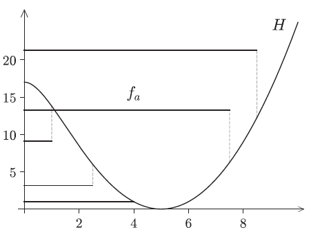
This situation is illustrated in Figure 1, where the functions H and $f_a$ for several values of a are plotted, including $V=f_{a^*}$. Of course, $V=f_{a^*}$ is dominated by every other $f_a$. Note that each $f_a$ is constant for $y \in [0,a)$, since $Y^y$ moves upwards by jumps only, and that because of the lack of memory property of the exponentially distributed jumps, the overshoot over the level a does not depend on the position just prior to the jump causing the overshoot. It is further worth noting that $V=f_{a^*}$ is the only choice of $a \geq 0$ that results in a continuous function; for $a \not= a^*$ the function $f_a$ has a discontinuity at $y=a$. This phenomenon is well known in optimal stopping (for processes of bounded variation) and is usually referred to as ‘continuous fit’ or ‘continuous pasting’ (see e.g. [Reference Alili and Kyprianou2]).

Figure 1:

A plot of H and $f_a$ for several values of a for the bounded-variation process (4.1) with $c=0.5$, $\mu=1$, $\eta=1$, and $b=5$.

Next we add a Brownian motion B to the above example to create a process of unbounded variation:

(4.2) \begin{equation}X_t= \sigma B_t + ct-\sum_{k=1}^{N_t} Z_k \quad \text{for all $t \geq 0$.}\end{equation}

It is again easily verified that

\[ \psi(z)=\frac{\sigma^2}{2} z^2 + cz-\frac{\mu z}{z+\eta} \quad \text{with domain $(-\eta,\infty)$} \]

(see also e.g. [Reference Kuznetsov, Kyprianou and Rivero16]), and denoting the three distinct roots of $\psi$ by $z_i$, we have

\[ W(x) = \frac{e^{z_1 x}}{\psi'(z_1)}+\frac{e^{z_2 x}}{\psi'(z_2)}+\frac{e^{z_3 x}}{\psi'(z_3)} \quad \text{for $x \geq 0$.} \]

Choosing $\sigma=1$, $c=0.5$, $\mu=1$, $\eta=1$, and $b=5$, we are again in Case (ii) of Theorem 2.1, and we can compute $a^* \approx 4.38<b=5$.

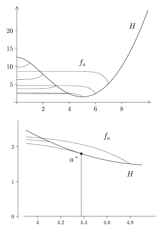
Figure 2 again shows plots of H and $f_a$ for several values of a. Noteworthy is that now all the $f_a$ are continuous, and that $V=f_{a^*}$ distinguishes itself from $f_a$ for other values of a via a $C^1$ fit to H at $y=a$ rather than only a continuous fit. This is known as ‘smooth fit’ or ‘smooth pasting’ (see again [Reference Alili and Kyprianou2], for example).

Figure 2:

A plot of H and $f_a$ for several values of a for the unbounded-variation process (4.2) with $\sigma=1$, $c=0.5$, $\mu=1$, $\eta=1$, and $b=5$.

Remark 4.1. It is worth noting that in Figures 1 and 2 the functions $f_a$ seem to have a vanishing derivative at $y=0$. Indeed a bit of algebra with the expressions from Lemma 3.2 reveals that in general $f_a'(0+)=0$. This property is usually referred to as ‘normal reflection’ or ‘instantaneous reflection’ (see e.g. [Reference Peskir and Shiryaev19, p. 264] or [Reference Du Toit and Peskir12, Equation (3.32)]) and naturally arises as follows. Using the strong Markov property it can be checked for any $t \geq 0$ that

\[ {\mathbb{E}} \left[ \left. H \left( Y^y_{\tau^y_a} \right) \, \right| \, \mathcal{F}_t \right] = f_a \left( Y^y_{t \wedge \tau^y_a} \right) =: Z_t, \]

i.e. that Z is martingale. (Note that the Snell envelope for our problem is contained in this family, for $a=y^*$.) If the normal reflection property did not hold, then the (local) time $Y^y$ accumulates at level 0 would destroy this martingale property. In a more purely free-boundary approach to problems of this type, normal reflection is typically included as one of the conditions imposed on the solution to the free boundary problem. However, in the approach we have chosen in this paper, where in particular the proofs only consider processes that are stopped before $Y^y$ hits the level 0, normal reflection appears as a property of the solution rather than as a condition imposed on the solution.