2 Inertial waves of finite amplitude in rotating fluids

We study the Euler equations in the reference frame, rotating with an incompressible fluid:

(2.1a ) $$\begin{eqnarray}\displaystyle & \displaystyle \unicode[STIX]{x2202}_{t}\boldsymbol{v}+(\boldsymbol{v}\boldsymbol{\cdot }\unicode[STIX]{x1D735})\boldsymbol{v}+2(\unicode[STIX]{x1D734}\times \boldsymbol{v})=-\unicode[STIX]{x1D735}P, & \displaystyle\end{eqnarray}$$

(2.1b ) $$\begin{eqnarray}\displaystyle & \displaystyle \unicode[STIX]{x1D735}\boldsymbol{\cdot }\boldsymbol{v}=0. & \displaystyle\end{eqnarray}$$

$P=p-(\unicode[STIX]{x1D734}\times \boldsymbol{r})^{2}/2$

$p$

$\propto \unicode[STIX]{x1D6FA}^{2}$

$2(\unicode[STIX]{x1D734}\times \boldsymbol{v})$

$\boldsymbol{r}=(x,y,z)$

$(\widehat{\boldsymbol{x}},\widehat{\boldsymbol{y}},\widehat{\boldsymbol{z}})$

$\unicode[STIX]{x1D734}\Vert \widehat{\boldsymbol{z}}$

The nonlinearity of the Euler equations affects only the waves moving in different directions, which is a general consequence of incompressibility for unbounded flows (see, for instance, Craik & Criminale (Reference Craik and Criminale1986)). Indeed, the plane inertial wave (as well as a package of such waves propagating in the same direction) is the exact solution of (2.1). Because this fact is often overlooked in recent papers (except, to the best of our knowledge, the paper of Messio et al. (Reference Messio, Morize, Rabaud and Moisy2008)), we discuss it here in more detail.

We consider the general solution of (2.1) under the assumption that the velocity field $\boldsymbol{v}$ depends only on the coordinate $\unicode[STIX]{x1D709}$ along an arbitrary direction $\boldsymbol{n}$ . Bearing in mind the axial symmetry around $\widehat{\boldsymbol{z}}$ , we can choose $\boldsymbol{n}$ lying in the $xz$ -plane so that

(2.2a-c ) $$\begin{eqnarray}\boldsymbol{n}=(\sin \unicode[STIX]{x1D703},0,\cos \unicode[STIX]{x1D703}),\quad \unicode[STIX]{x1D709}=\boldsymbol{r}\boldsymbol{\cdot }\boldsymbol{n},\quad \boldsymbol{v}(\boldsymbol{r},t)\equiv \boldsymbol{v}(\unicode[STIX]{x1D709},t)=\boldsymbol{v}(x\sin \unicode[STIX]{x1D703}+z\cos \unicode[STIX]{x1D703},t).\end{eqnarray}$$

Then, integrating the continuity equation (2.1b ) by $\unicode[STIX]{x1D709}$ , we find

(2.3) $$\begin{eqnarray}v_{z}=-v_{x}\tan \unicode[STIX]{x1D703}.\end{eqnarray}$$

We neglect the integration constant, which corresponds to steady motion of the whole fluid along $\widehat{\boldsymbol{z}}$ . Thus, the nonlinear term in (2.1a ) is exactly cancelled:

(2.4) $$\begin{eqnarray}(\boldsymbol{v}\boldsymbol{\cdot }\unicode[STIX]{x1D735})\boldsymbol{v}=(v_{x}\sin \unicode[STIX]{x1D703}+v_{z}\cos \unicode[STIX]{x1D703})\frac{\unicode[STIX]{x2202}\boldsymbol{v}}{\unicode[STIX]{x2202}\unicode[STIX]{x1D709}}\equiv 0.\end{eqnarray}$$

Now, the equation (2.1) can be written as the following system of linear equations:

(2.5) $$\begin{eqnarray}\displaystyle \left.\begin{array}{@{}c@{}}\displaystyle \frac{\unicode[STIX]{x2202}v_{x}}{\unicode[STIX]{x2202}t}-2\unicode[STIX]{x1D6FA}v_{y}+\sin \unicode[STIX]{x1D703}\frac{\unicode[STIX]{x2202}P}{\unicode[STIX]{x2202}\unicode[STIX]{x1D709}}=0,\\ \displaystyle \frac{\unicode[STIX]{x2202}v_{y}}{\unicode[STIX]{x2202}t}+2\unicode[STIX]{x1D6FA}v_{x}=0,\\ \displaystyle \frac{\unicode[STIX]{x2202}v_{z}}{\unicode[STIX]{x2202}t}+\cos \unicode[STIX]{x1D703}\frac{\unicode[STIX]{x2202}P}{\unicode[STIX]{x2202}\unicode[STIX]{x1D709}}=0.\end{array}\right\} & & \displaystyle\end{eqnarray}$$

By using (2.3), we find the exact solution for the system (2.5):

(2.6) $$\begin{eqnarray}\displaystyle \left.\begin{array}{@{}c@{}}\displaystyle v_{x}=-A(\unicode[STIX]{x1D709})\cos \unicode[STIX]{x1D703}\sin \unicode[STIX]{x1D714}t-B(\unicode[STIX]{x1D709})\cos \unicode[STIX]{x1D703}\cos \unicode[STIX]{x1D714}t,\\ \displaystyle v_{y}=-A(\unicode[STIX]{x1D709})\cos \unicode[STIX]{x1D714}t+B(\unicode[STIX]{x1D709})\sin \unicode[STIX]{x1D714}t,\\ \displaystyle v_{z}=A(\unicode[STIX]{x1D709})\sin \unicode[STIX]{x1D703}\sin \unicode[STIX]{x1D714}t+B(\unicode[STIX]{x1D709})\sin \unicode[STIX]{x1D703}\cos \unicode[STIX]{x1D714}t.\end{array}\right\} & & \displaystyle\end{eqnarray}$$

Here, $\unicode[STIX]{x1D714}=2\unicode[STIX]{x1D6FA}|\text{cos}\,\unicode[STIX]{x1D703}|$ , while $A(\unicode[STIX]{x1D709})$ and $B(\unicode[STIX]{x1D709})$ are arbitrary functions. Solution (2.6) is the wave packet of plane inertial waves propagating along $\boldsymbol{n}$ . We now introduce the wave vector $\boldsymbol{k}\Vert \boldsymbol{n}$ . Choosing $A(\unicode[STIX]{x1D709})=A\sin (\boldsymbol{k}\boldsymbol{\cdot }\boldsymbol{r}),B(\unicode[STIX]{x1D709})=A\cos (\boldsymbol{k}\boldsymbol{\cdot }\boldsymbol{r})$ , we obtain the well-known circularly polarized inertial plane wave solution (Landau & Lifshitz Reference Landau and Lifshitz1987):

(2.7) $$\begin{eqnarray}\displaystyle \left.\begin{array}{@{}c@{}}\displaystyle v_{x}=-A\cos \unicode[STIX]{x1D703}_{\boldsymbol{k}}\cos (\unicode[STIX]{x1D714}_{\boldsymbol{k}}t-\boldsymbol{k}\boldsymbol{\cdot }\boldsymbol{r}),\\ \displaystyle v_{y}=A\sin (\unicode[STIX]{x1D714}_{\boldsymbol{k}}t-\boldsymbol{k}\boldsymbol{\cdot }\boldsymbol{r}),\\ \displaystyle v_{z}=A\sin \unicode[STIX]{x1D703}_{\boldsymbol{k}}\cos (\unicode[STIX]{x1D714}_{\boldsymbol{k}}t-\boldsymbol{k}\boldsymbol{\cdot }\boldsymbol{r}).\end{array}\right\} & & \displaystyle\end{eqnarray}$$

The expression (2.6) gives the exact class of finite amplitude solutions of the Euler equations in the rotating reference frame (2.1).

3 Hamiltonian description of inertial waves

3.1 Clebsch representation of the velocity field

The Euler equations for incompressible fluids can be written as a Hamiltonian system using the so-called Clebsch variables $\unicode[STIX]{x1D706}(\boldsymbol{r},t)$ and $\unicode[STIX]{x1D707}(\boldsymbol{r},t)$  (Lamb Reference Lamb1945). Here, we find the following Clebsch representation for the velocity field $\boldsymbol{v}(\boldsymbol{r},t)$ corresponding to the case of a rotating fluid described by (2.1):

(3.1) $$\begin{eqnarray}\displaystyle \boldsymbol{v}(\boldsymbol{r},t)=\sqrt{2\unicode[STIX]{x1D6FA}}[\widehat{\boldsymbol{y}}\unicode[STIX]{x1D706}(\boldsymbol{r},t)-\widehat{\boldsymbol{x}}\unicode[STIX]{x1D707}(\boldsymbol{r},t)]+\unicode[STIX]{x1D706}(\boldsymbol{r},t)\unicode[STIX]{x1D735}\unicode[STIX]{x1D707}(\boldsymbol{r},t)+\unicode[STIX]{x1D735}\unicode[STIX]{x1D6F7}(\boldsymbol{r},t), & & \displaystyle\end{eqnarray}$$

(remember that $\unicode[STIX]{x1D734}\Vert \widehat{\boldsymbol{z}}$ ). The potential $\unicode[STIX]{x1D6F7}(\boldsymbol{r},t)$ is uniquely determined from the appropriate boundary conditions and the continuity equation (2.1b ). Similar variables were introduced by Zakharov (Reference Zakharov1971) and by Kuznetsov (Reference Kuznetsov1972) in the theory of magnetized plasma. The last two terms in (3.1) correspond to the standard Clebsch representation in the case of a non-rotating fluid. The first term appears as a result of the transformation from an inertial to a rotating reference frame (see the details in appendix A).

Alternatively, the velocity field $\boldsymbol{v}(\boldsymbol{r},t)$ can be written using the transverse projector

(3.2) $$\begin{eqnarray}\widehat{\boldsymbol{P}}\equiv 1-\unicode[STIX]{x1D735}\unicode[STIX]{x1D6E5}^{-1}\unicode[STIX]{x1D735},\end{eqnarray}$$

as (see appendix A)

(3.3) $$\begin{eqnarray}\boldsymbol{v}=\widehat{\boldsymbol{P}}\boldsymbol{\cdot }[\sqrt{2\unicode[STIX]{x1D6FA}}(\unicode[STIX]{x1D706}\widehat{\boldsymbol{y}}-\unicode[STIX]{x1D707}\widehat{\boldsymbol{x}})+\unicode[STIX]{x1D706}\unicode[STIX]{x1D735}\unicode[STIX]{x1D707}].\end{eqnarray}$$

The fields $\unicode[STIX]{x1D706}(\boldsymbol{r},t)$ and $\unicode[STIX]{x1D707}(\boldsymbol{r},t)$ are not uniquely defined for a particular velocity field $\boldsymbol{v}(\boldsymbol{r},t)$ . For instance, the transformation with arbitrary constant parameters $a$ , $b$ and $c$ ,

(3.4a,b ) $$\begin{eqnarray}\unicode[STIX]{x1D706}(\boldsymbol{r},t)\rightarrow a\unicode[STIX]{x1D706}(\boldsymbol{r},t)+b,\quad \unicode[STIX]{x1D707}(\boldsymbol{r},t)\rightarrow \unicode[STIX]{x1D707}(\boldsymbol{r},t)/a+c,\end{eqnarray}$$

does not change the field $\boldsymbol{v}$ given by (3.1). This type of ‘gauge invariance’ enables the selection of special calibration for the Clebsch variables $\unicode[STIX]{x1D706}(\boldsymbol{r},t)$ and $\unicode[STIX]{x1D707}(\boldsymbol{r},t)$ , which is ideal for solving a particular problem.

The fields $\unicode[STIX]{x1D706}(\boldsymbol{r},t),\unicode[STIX]{x1D707}(\boldsymbol{r},t)$ obey the Hamiltonian equations of motion in the canonical form:

(3.5a,b ) $$\begin{eqnarray}\unicode[STIX]{x2202}_{t}\unicode[STIX]{x1D706}=\frac{\unicode[STIX]{x1D6FF}{\mathcal{H}}}{\unicode[STIX]{x1D6FF}\unicode[STIX]{x1D707}},\quad \unicode[STIX]{x2202}_{t}\unicode[STIX]{x1D707}=-\frac{\unicode[STIX]{x1D6FF}{\mathcal{H}}}{\unicode[STIX]{x1D6FF}\unicode[STIX]{x1D706}},\end{eqnarray}$$

where $\unicode[STIX]{x1D6FF}$ is the variational derivative, and the Hamiltonian ${\mathcal{H}}$ is the energy represented by $\unicode[STIX]{x1D706}$ and $\unicode[STIX]{x1D707}$ :

(3.6) $$\begin{eqnarray}{\mathcal{H}}=\int \frac{1}{2}|\boldsymbol{v}|^{2}\,\text{d}\boldsymbol{r}.\end{eqnarray}$$

Equations (3.5) and (3.6) yield

(3.7a ) $$\begin{eqnarray}\displaystyle & \displaystyle \unicode[STIX]{x2202}_{t}\unicode[STIX]{x1D706}=-(\boldsymbol{v}\boldsymbol{\cdot }\unicode[STIX]{x1D735})\unicode[STIX]{x1D706}-\sqrt{2\unicode[STIX]{x1D6FA}}v_{x}, & \displaystyle\end{eqnarray}$$

(3.7b ) $$\begin{eqnarray}\displaystyle & \displaystyle \unicode[STIX]{x2202}_{t}\unicode[STIX]{x1D707}=-(\boldsymbol{v}\boldsymbol{\cdot }\unicode[STIX]{x1D735})\unicode[STIX]{x1D707}-\sqrt{2\unicode[STIX]{x1D6FA}}v_{y}. & \displaystyle\end{eqnarray}$$

From equations (3.1) and (3.7), we find that $\boldsymbol{v}$ satisfies the Euler equations (2.1) with the effective pressure

(3.8) $$\begin{eqnarray}P=-\unicode[STIX]{x2202}_{t}\unicode[STIX]{x1D6F7}-\unicode[STIX]{x1D706}\unicode[STIX]{x2202}_{t}\unicode[STIX]{x1D707}-{\textstyle \frac{1}{2}}|\boldsymbol{v}|^{2}-{\textstyle \frac{1}{2}}(\unicode[STIX]{x1D734}\times \boldsymbol{r})^{2}.\end{eqnarray}$$

3.2 Hamiltonian in a rotating reference frame

Let us introduce the following notation for the velocity field (3.3):

(3.9a-c ) $$\begin{eqnarray}\boldsymbol{v}=\boldsymbol{v}_{1}+\boldsymbol{v}_{2},\quad \boldsymbol{v}_{1}=\widehat{\boldsymbol{P}}\boldsymbol{\cdot }[\sqrt{2\unicode[STIX]{x1D6FA}}(\unicode[STIX]{x1D706}\widehat{\boldsymbol{y}}-\unicode[STIX]{x1D707}\widehat{\boldsymbol{x}})],\quad \boldsymbol{v}_{2}=\widehat{\boldsymbol{P}}\boldsymbol{\cdot }(\unicode[STIX]{x1D706}\unicode[STIX]{x1D735}\unicode[STIX]{x1D707}),\end{eqnarray}$$

and symmetric Fourier transform:

(3.10a,b ) $$\begin{eqnarray}\displaystyle \boldsymbol{v}_{\boldsymbol{k}}=\frac{1}{(2\unicode[STIX]{x03C0})^{3/2}}\int \boldsymbol{v}\exp (-\text{i}\boldsymbol{k}\boldsymbol{\cdot }\boldsymbol{r})\,\text{d}\boldsymbol{r},\quad \boldsymbol{v}=\frac{1}{(2\unicode[STIX]{x03C0})^{3/2}}\int \boldsymbol{v}_{\boldsymbol{k}}\exp (\text{i}\boldsymbol{k}\boldsymbol{\cdot }\boldsymbol{r})\,\text{d}\boldsymbol{k}. & & \displaystyle\end{eqnarray}$$

By representation (3.9), we distinguish the impact of linear and nonlinear combinations ( $\boldsymbol{v}_{1}$ and $\boldsymbol{v}_{1}$ respectively) of the Clebsch variables $\unicode[STIX]{x1D706}$ and $\unicode[STIX]{x1D707}$ on the velocity field. According to (3.6) and Parseval’s theorem, the Hamiltonian can be written as the sum of the following three terms:

(3.11a ) $$\begin{eqnarray}\displaystyle {\mathcal{H}}={\mathcal{H}}_{2}+{\mathcal{H}}_{3}+{\mathcal{H}}_{4}. & & \displaystyle\end{eqnarray}$$

Here

(3.11b ) $$\begin{eqnarray}\displaystyle & \displaystyle {\mathcal{H}}_{2}=\frac{1}{2}\int |\boldsymbol{v}_{1\boldsymbol{k}}|^{2}\,\text{d}\boldsymbol{k}, & \displaystyle\end{eqnarray}$$

(3.11c ) $$\begin{eqnarray}\displaystyle & \displaystyle {\mathcal{H}}_{3}=\frac{1}{2}\int (\boldsymbol{v}_{1\boldsymbol{k}}\boldsymbol{\cdot }\boldsymbol{v}_{2\boldsymbol{k}}^{\ast }+\boldsymbol{v}_{1\boldsymbol{k}}^{\ast }\boldsymbol{\cdot }\boldsymbol{v}_{2\boldsymbol{k}})\,\text{d}\boldsymbol{k}, & \displaystyle\end{eqnarray}$$

(3.11d ) $$\begin{eqnarray}\displaystyle & \displaystyle {\mathcal{H}}_{4}=\int |\boldsymbol{v}_{2\boldsymbol{k}}|^{2}\,\text{d}\boldsymbol{k}. & \displaystyle\end{eqnarray}$$

The interactions of inertial waves are described by ${\mathcal{H}}_{3}$ and ${\mathcal{H}}_{4}$ , which we denote as interaction Hamiltonian

(3.12) $$\begin{eqnarray}{\mathcal{H}}_{int}={\mathcal{H}}_{3}+{\mathcal{H}}_{4}.\end{eqnarray}$$

The expression (3.11) is the exact Hamiltonian for an ideal rotating incompressible fluid. It contains a finite number of terms since for incompressible flow we use only one pair of canonical variables $\unicode[STIX]{x1D706}(\boldsymbol{r},t)$ and $\unicode[STIX]{x1D707}(\boldsymbol{r},t)$ (see the corresponding discussion in Zakharov et al. (Reference Zakharov, L’vov and Falkovich1992)).

Now, let us denote the components of wave vector $\boldsymbol{k}$ as

(3.13a,b ) $$\begin{eqnarray}\displaystyle \boldsymbol{k}=(k_{x},k_{y},k_{z})=(k\sin \unicode[STIX]{x1D703}\cos \unicode[STIX]{x1D711},k\sin \unicode[STIX]{x1D703}\sin \unicode[STIX]{x1D711},k\cos \unicode[STIX]{x1D703}),\quad \boldsymbol{k}_{\bot }=(k_{x},k_{y}). & & \displaystyle\end{eqnarray}$$

Using the expression for transverse projector $\widehat{P}$ in $\boldsymbol{k}$ -space

(3.14) $$\begin{eqnarray}\widehat{P}_{\boldsymbol{k}}^{\unicode[STIX]{x1D6FC}\unicode[STIX]{x1D6FD}}=\unicode[STIX]{x1D6FF}^{\unicode[STIX]{x1D6FC}\unicode[STIX]{x1D6FD}}-\frac{k^{\unicode[STIX]{x1D6FC}}k^{\unicode[STIX]{x1D6FD}}}{k^{2}},\end{eqnarray}$$

and equation (3.9), we calculate the following Fourier components of the velocity field:

(3.15a ) $$\begin{eqnarray}\displaystyle & \displaystyle \boldsymbol{v}_{1\boldsymbol{k}}=\sqrt{2\unicode[STIX]{x1D6FA}}\left[\unicode[STIX]{x1D706}_{\boldsymbol{k}}\widehat{\boldsymbol{y}}-\unicode[STIX]{x1D707}_{\boldsymbol{k}}\widehat{\boldsymbol{x}}-\frac{\boldsymbol{k}}{k^{2}}(k_{y}\unicode[STIX]{x1D706}_{\boldsymbol{k}}-k_{x}\unicode[STIX]{x1D707}_{\boldsymbol{k}})\right], & \displaystyle\end{eqnarray}$$

(3.15b ) $$\begin{eqnarray}\displaystyle & \displaystyle \boldsymbol{v}_{2\boldsymbol{k}}=\frac{\text{i}}{(2\unicode[STIX]{x03C0})^{3/2}}\int \left(\boldsymbol{k}_{2}-\boldsymbol{k}\frac{\boldsymbol{k}\boldsymbol{\cdot }\boldsymbol{k}_{2}}{k^{2}}\right)\unicode[STIX]{x1D706}_{\boldsymbol{k}_{1}}\unicode[STIX]{x1D707}_{\boldsymbol{k}_{2}}\unicode[STIX]{x1D6FF}_{\boldsymbol{k}-\boldsymbol{k}_{1}-\boldsymbol{k}_{2}}\,\text{d}\boldsymbol{k}_{1}\,\text{d}\boldsymbol{k}_{2}. & \displaystyle\end{eqnarray}$$

When $\boldsymbol{k}\Vert \boldsymbol{k}_{1}\Vert \boldsymbol{k}_{2}$ , the expression $\boldsymbol{k}_{2}-\boldsymbol{k}(\boldsymbol{k}\boldsymbol{\cdot }\boldsymbol{k}_{2}/k^{2})$ in (3.15b ) is exactly zero, according to the conservation law: $\boldsymbol{k}-\boldsymbol{k}_{1}-\boldsymbol{k}_{2}=0$ . Thus, in this case, the interaction Hamiltonian ${\mathcal{H}}_{int}=0$ , which again demonstrates that inertial waves moving in one direction do not interact (see § 2).

3.3 Canonical form of the quadratic Hamiltonian

We now introduce the following canonical transformation of the fields $\unicode[STIX]{x1D707}_{\boldsymbol{k}}$ and $\unicode[STIX]{x1D706}_{\boldsymbol{k}}$ in $\boldsymbol{k}$ -space:

(3.16) $$\begin{eqnarray}\displaystyle \left.\begin{array}{@{}c@{}}\displaystyle \unicode[STIX]{x1D707}_{\boldsymbol{k}}=\widetilde{\unicode[STIX]{x1D707}}_{\boldsymbol{k}}\cos \unicode[STIX]{x1D711}+\widetilde{\unicode[STIX]{x1D706}}_{\boldsymbol{k}}\sin \unicode[STIX]{x1D711}=\frac{1}{k_{\bot }}(\widetilde{\unicode[STIX]{x1D707}}_{\boldsymbol{k}}k_{x}+\widetilde{\unicode[STIX]{x1D706}}_{\boldsymbol{k}}k_{y}),\\ \displaystyle \unicode[STIX]{x1D706}_{\boldsymbol{k}}=-\widetilde{\unicode[STIX]{x1D707}}_{\boldsymbol{k}}\sin \unicode[STIX]{x1D711}+\widetilde{\unicode[STIX]{x1D706}}_{k}\cos \unicode[STIX]{x1D711}=\frac{1}{k_{\bot }}(-\widetilde{\unicode[STIX]{x1D707}}_{\boldsymbol{k}}k_{y}+\widetilde{\unicode[STIX]{x1D706}}_{\boldsymbol{k}}k_{x}).\end{array}\right\} & & \displaystyle\end{eqnarray}$$

Introducing the normal variables $c_{\boldsymbol{k}}$ and $c_{\boldsymbol{k}}^{\ast }$ ,

(3.17a,b ) $$\begin{eqnarray}\widetilde{\unicode[STIX]{x1D707}}_{\boldsymbol{k}}=\sqrt{\frac{\unicode[STIX]{x1D6FA}}{\unicode[STIX]{x1D714}_{\boldsymbol{k}}}}(c_{\boldsymbol{k}}+c_{-\boldsymbol{k}}^{\ast }),\quad \widetilde{\unicode[STIX]{x1D706}}_{\boldsymbol{ k}}=-\frac{\text{i}}{2}\sqrt{\frac{\unicode[STIX]{x1D714}_{\boldsymbol{k}}}{\unicode[STIX]{x1D6FA}}}(c_{\boldsymbol{k}}-c_{-\boldsymbol{k}}^{\ast }),\end{eqnarray}$$

we present the quadratic part of the Hamiltonian ${\mathcal{H}}_{2}$ in diagonal form:

(3.18a,b ) $$\begin{eqnarray}{\mathcal{H}}_{2}=\int \unicode[STIX]{x1D714}_{\boldsymbol{k}}c_{\boldsymbol{k}}c_{\boldsymbol{k}}^{\ast }\,\text{d}\boldsymbol{k},\quad \unicode[STIX]{x1D714}_{\boldsymbol{ k}}=2\unicode[STIX]{x1D6FA}|\text{cos}\,\unicode[STIX]{x1D703}_{\boldsymbol{k}}|.\end{eqnarray}$$

The plane wave in normal variables corresponds to the operator

(3.19) $$\begin{eqnarray}c_{k}=A\text{e}^{\text{i}\unicode[STIX]{x1D714}_{k}t}\unicode[STIX]{x1D6FF}(\boldsymbol{k}-\boldsymbol{k}_{0}).\end{eqnarray}$$

By substituting (3.19) into (3.17) and then into (3.16) and finally calculating the linear part of the velocity field equation (3.15a ), we recover the plane inertial wave solution (2.7) multiplied by scalar factor $(k_{x}/k_{\bot })\sqrt{\unicode[STIX]{x1D714}_{\boldsymbol{k}}}$ . This normalization of the plane wave solution in variables $c_{\boldsymbol{k}}$ and $c_{\boldsymbol{k}}^{\ast }$ should be taken into account when comparing the results of this paper with the predictions of approaches formulated with physical variables.

3.4 Interaction Hamiltonian

We calculate the interaction Hamiltonian ${\mathcal{H}}_{int}$ in two steps. First, we calculate ${\mathcal{H}}_{3}$ and ${\mathcal{H}}_{4}$ in variables $\widetilde{\unicode[STIX]{x1D707}}_{\boldsymbol{k}}$ and $\widetilde{\unicode[STIX]{x1D706}}_{\boldsymbol{k}}$ according to (3.11c ), (3.15a ), (3.15b ) and (3.16). After symmetrization, ${\mathcal{H}}_{3}$ takes the form

(3.20) $$\begin{eqnarray}\displaystyle {\mathcal{H}}_{3} & = & \displaystyle \frac{\text{i}\sqrt{2\unicode[STIX]{x1D6FA}}}{2(2\unicode[STIX]{x03C0})^{3/2}}\int \frac{\text{d}\boldsymbol{k}_{1}\,\text{d}\boldsymbol{k}_{2}\,\text{d}\boldsymbol{k}_{3}}{k_{1\bot }k_{2\bot }k_{3\bot }}\unicode[STIX]{x1D6FF}_{\boldsymbol{k}_{1}-\boldsymbol{k}_{2}-\boldsymbol{k}_{3}}(F_{\boldsymbol{k}_{2}\boldsymbol{k}_{3}}^{\boldsymbol{k}_{1}}\unicode[STIX]{x1D707}_{\boldsymbol{k}_{1}}-S_{\boldsymbol{k}_{2}\boldsymbol{k}_{3}}\unicode[STIX]{x1D706}_{\boldsymbol{k}_{1}})\nonumber\\ \displaystyle & & \displaystyle \times \,[S_{\boldsymbol{k}_{2}\boldsymbol{k}_{3}}(\unicode[STIX]{x1D707}_{\boldsymbol{k}_{2}}\unicode[STIX]{x1D707}_{\boldsymbol{k}_{3}}+\unicode[STIX]{x1D706}_{\boldsymbol{k}_{2}}\unicode[STIX]{x1D706}_{\boldsymbol{k}_{3}})+(\boldsymbol{k}_{2\bot }\boldsymbol{\cdot }\boldsymbol{k}_{3\bot })(\unicode[STIX]{x1D707}_{\boldsymbol{k}_{2}}\unicode[STIX]{x1D706}_{\boldsymbol{k}_{3}}-\unicode[STIX]{x1D706}_{\boldsymbol{k}_{2}}\unicode[STIX]{x1D707}_{\boldsymbol{k}_{3}})].\end{eqnarray}$$

Here, we use the auxiliary functions

(3.21) $$\begin{eqnarray}\displaystyle \left.\begin{array}{@{}c@{}}\displaystyle F_{\boldsymbol{k}_{2}\boldsymbol{k}_{3}}^{\boldsymbol{k}_{1}}=\frac{1}{2}\left[k_{1\bot }^{2}\frac{\boldsymbol{k}_{1}\boldsymbol{\cdot }\boldsymbol{k}_{2}-\boldsymbol{k}_{1}\boldsymbol{\cdot }\boldsymbol{k}_{3}}{k_{1}^{2}}+k_{2\bot }^{2}-k_{3\bot }^{2}\right],\\ \displaystyle S_{\boldsymbol{k}_{2}\boldsymbol{k}_{3}}=k_{3x}k_{2y}-k_{2x}k_{3y}=k_{2\bot }k_{3\bot }\sin (\unicode[STIX]{x1D711}_{2}-\unicode[STIX]{x1D711}_{3}),\end{array}\right\} & & \displaystyle\end{eqnarray}$$

with the following properties:

(3.22a-c ) $$\begin{eqnarray}\displaystyle F_{\boldsymbol{k}_{l}\boldsymbol{k}_{m}}^{\boldsymbol{k}_{i}}=-F_{\boldsymbol{ k}_{m}\boldsymbol{k}_{l}}^{\boldsymbol{k}_{i}},\quad S_{\boldsymbol{ k}_{l}\boldsymbol{k}_{m}}=-S_{\boldsymbol{k}_{m}\boldsymbol{k}_{l}},\quad S_{\boldsymbol{k}_{2},\boldsymbol{k}_{3}}=S_{\boldsymbol{k}_{3},\boldsymbol{k}_{1}}=S_{\boldsymbol{k}_{1},\boldsymbol{k}_{2}}. & & \displaystyle\end{eqnarray}$$

For the ${\mathcal{H}}_{4}$ component of the interaction Hamiltonian, we find the following expression:

(3.23) $$\begin{eqnarray}\displaystyle {\mathcal{H}}_{4} & = & \displaystyle \frac{1}{4(2\unicode[STIX]{x03C0})^{3}}\int \frac{\text{d}\boldsymbol{k}_{1}\,\text{d}\boldsymbol{k}_{2}\,\text{d}\boldsymbol{k}_{3}\,\text{d}\boldsymbol{k}_{4}}{k_{1\bot }k_{2\bot }k_{3\bot }k_{4\bot }}\unicode[STIX]{x1D6FF}_{\boldsymbol{k}_{1}+\boldsymbol{k}_{2}-\boldsymbol{k}_{3}-\boldsymbol{k}_{4}}Q_{\boldsymbol{k}_{3}\boldsymbol{k}_{4}}^{\boldsymbol{k}_{1}\boldsymbol{k}_{2}}\nonumber\\ \displaystyle & & \displaystyle \times \,[S_{\boldsymbol{k}_{1}\boldsymbol{k}_{2}}(\unicode[STIX]{x1D707}_{\boldsymbol{k}_{1}}\unicode[STIX]{x1D707}_{\boldsymbol{k}_{2}}+\unicode[STIX]{x1D706}_{\boldsymbol{k}_{1}}\unicode[STIX]{x1D706}_{\boldsymbol{k}_{2}})+(\boldsymbol{k}_{1\bot }\boldsymbol{\cdot }\boldsymbol{k}_{2\bot })(\unicode[STIX]{x1D707}_{\boldsymbol{k}_{1}}\unicode[STIX]{x1D706}_{\boldsymbol{k}_{2}}-\unicode[STIX]{x1D706}_{\boldsymbol{k}_{1}}\unicode[STIX]{x1D707}_{\boldsymbol{k}_{2}})]\nonumber\\ \displaystyle & & \displaystyle \times \,[S_{\boldsymbol{k}_{3}\boldsymbol{k}_{4}}(\unicode[STIX]{x1D707}_{\boldsymbol{k}_{3}}\unicode[STIX]{x1D707}_{\boldsymbol{k}_{4}}+\unicode[STIX]{x1D706}_{\boldsymbol{k}_{3}}\unicode[STIX]{x1D706}_{\boldsymbol{k}_{4}})+(\boldsymbol{k}_{3\bot }\boldsymbol{\cdot }\boldsymbol{k}_{4\bot })(\unicode[STIX]{x1D707}_{\boldsymbol{k}_{3}}\unicode[STIX]{x1D706}_{\boldsymbol{k}_{4}}-\unicode[STIX]{x1D706}_{\boldsymbol{k}_{3}}\unicode[STIX]{x1D707}_{\boldsymbol{k}_{4}})].\end{eqnarray}$$

Here, we use the additional function

(3.24) $$\begin{eqnarray}Q_{\boldsymbol{k}_{3}\boldsymbol{k}_{4}}^{\boldsymbol{ k}_{1}\boldsymbol{ k}_{2}}=\frac{(\boldsymbol{k}_{1}\boldsymbol{\cdot }\boldsymbol{k}_{3})(\boldsymbol{k}_{2}\boldsymbol{\cdot }\boldsymbol{k}_{4})-(\boldsymbol{k}_{1}\boldsymbol{\cdot }\boldsymbol{k}_{4})(\boldsymbol{k}_{2}\boldsymbol{\cdot }\boldsymbol{k}_{3})}{(\boldsymbol{k}_{1}+\boldsymbol{k}_{2})\boldsymbol{\cdot }(\boldsymbol{k}_{3}+\boldsymbol{k}_{4})}.\end{eqnarray}$$

The function $Q_{\boldsymbol{k}_{3}\boldsymbol{k}_{4}}^{\boldsymbol{k}_{1}\boldsymbol{k}_{2}}$ is antisymmetric with respect to the transformations $\boldsymbol{k}_{1}\leftrightarrow \boldsymbol{k}_{2}$ and $\boldsymbol{k}_{3}\leftrightarrow \boldsymbol{k}_{4}$ :

(3.25a,b ) $$\begin{eqnarray}Q_{\boldsymbol{k}_{3}\boldsymbol{k}_{4}}^{\boldsymbol{ k}_{1}\boldsymbol{ k}_{2}}=-Q_{\boldsymbol{k}_{3}\boldsymbol{k}_{4}}^{\boldsymbol{ k}_{2}\boldsymbol{ k}_{1}},\quad Q_{\boldsymbol{k}_{3}\boldsymbol{k}_{4}}^{\boldsymbol{ k}_{1}\boldsymbol{ k}_{2}}=-Q_{\boldsymbol{k}_{4}\boldsymbol{k}_{3}}^{\boldsymbol{ k}_{1}\boldsymbol{ k}_{2}}.\end{eqnarray}$$

The interaction Hamiltonian is obviously invariant with respect to rotations by angle $\unicode[STIX]{x1D711}$ (i.e. around $\widehat{\boldsymbol{z}}$ ), which can be directly seen from expressions (3.20) and (3.23).

Then, we substitute the normal variables (3.17) into (3.20), and after symmetrization, ${\mathcal{H}}_{3}$ takes the standard form:

(3.26) $$\begin{eqnarray}\displaystyle {\mathcal{H}}_{3} & = & \displaystyle \frac{1}{2}\int (V_{\boldsymbol{k}_{2}\boldsymbol{k}_{3}}^{\boldsymbol{k}_{1}}c_{\boldsymbol{ k}_{1}}^{\ast }c_{\boldsymbol{ k}_{2}}c_{\boldsymbol{k}_{3}}+\text{c.c.})\unicode[STIX]{x1D6FF}_{\boldsymbol{k}_{1}-\boldsymbol{k}_{2}-\boldsymbol{k}_{3}}\,\text{d}\boldsymbol{k}_{1}\,\text{d}\boldsymbol{k}_{2}\,\text{d}\boldsymbol{k}_{3}\nonumber\\ \displaystyle & & \displaystyle +\,\frac{1}{6}\int (U_{\boldsymbol{k}_{1}\boldsymbol{k}_{2}\boldsymbol{k}_{3}}c_{\boldsymbol{k}_{1}}^{\ast }c_{\boldsymbol{k}_{2}}^{\ast }c_{\boldsymbol{k}_{3}}^{\ast }+\text{c.c.})\unicode[STIX]{x1D6FF}_{\boldsymbol{k}_{1}+\boldsymbol{k}_{2}+\boldsymbol{k}_{3}}\,\text{d}\boldsymbol{k}_{1}\,\text{d}\boldsymbol{k}_{2}\,\text{d}\boldsymbol{k}_{3},\end{eqnarray}$$

where

(3.27) $$\begin{eqnarray}\displaystyle V_{\boldsymbol{k}_{2}\boldsymbol{k}_{3}}^{\boldsymbol{k}_{1}} & = & \displaystyle \frac{\text{i}\sqrt{2\unicode[STIX]{x1D6FA}}}{(2\unicode[STIX]{x03C0})^{3/2}k_{1\bot }k_{2\bot }k_{3\bot }}\left\{\sqrt{\frac{\unicode[STIX]{x1D6FA}^{3}}{\unicode[STIX]{x1D714}_{\boldsymbol{k}_{1}}\unicode[STIX]{x1D714}_{\boldsymbol{k}_{2}}\unicode[STIX]{x1D714}_{\boldsymbol{k}_{3}}}}S_{\boldsymbol{k}_{3}\boldsymbol{k}_{2}}[F_{\boldsymbol{k}_{2}\boldsymbol{k}_{3}}^{\boldsymbol{k}_{1}}-F_{\boldsymbol{ k}_{1}\boldsymbol{k}_{3}}^{\boldsymbol{k}_{2}}-F_{\boldsymbol{ k}_{2}\boldsymbol{k}_{1}}^{\boldsymbol{k}_{3}}]\right.\nonumber\\ \displaystyle & & \displaystyle -\,\frac{3\text{i}}{8}\sqrt{\frac{\unicode[STIX]{x1D714}_{\boldsymbol{k}_{1}}\unicode[STIX]{x1D714}_{\boldsymbol{k}_{2}}\unicode[STIX]{x1D714}_{\boldsymbol{k}_{3}}}{\unicode[STIX]{x1D6FA}^{3}}}S_{\boldsymbol{k}_{3}\boldsymbol{k}_{2}}^{2}+\frac{\text{i}}{2}\sqrt{\frac{\unicode[STIX]{x1D6FA}}{\unicode[STIX]{x1D714}_{\boldsymbol{ k}_{1}}\unicode[STIX]{x1D714}_{\boldsymbol{k}_{2}}\unicode[STIX]{x1D714}_{\boldsymbol{k}_{3}}}}(\unicode[STIX]{x1D714}_{\boldsymbol{k}_{1}}-\unicode[STIX]{x1D714}_{\boldsymbol{k}_{2}}-\unicode[STIX]{x1D714}_{\boldsymbol{k}_{3}})S_{\boldsymbol{k}_{3}\boldsymbol{k}_{2}}^{2}\nonumber\\ \displaystyle & & \displaystyle +\,\frac{1}{4}\sqrt{\frac{\unicode[STIX]{x1D714}_{\boldsymbol{k}_{2}}\unicode[STIX]{x1D714}_{\boldsymbol{k}_{3}}}{\unicode[STIX]{x1D6FA}\unicode[STIX]{x1D714}_{\boldsymbol{k}_{1}}}}S_{\boldsymbol{k}_{3}\boldsymbol{k}_{2}}[-F_{\boldsymbol{k}_{2}\boldsymbol{k}_{3}}^{\boldsymbol{k}_{1}}+\boldsymbol{k}_{1\bot }\boldsymbol{\cdot }\boldsymbol{k}_{3\bot }-\boldsymbol{k}_{1\bot }\boldsymbol{\cdot }\boldsymbol{k}_{2\bot }]\nonumber\\ \displaystyle & & \displaystyle -\,\frac{\text{i}}{2}\sqrt{\frac{\unicode[STIX]{x1D6FA}\unicode[STIX]{x1D714}_{\boldsymbol{k}_{1}}}{\unicode[STIX]{x1D714}_{\boldsymbol{k}_{2}}\unicode[STIX]{x1D714}_{\boldsymbol{k}_{3}}}}[-F_{\boldsymbol{k}_{2}\boldsymbol{k}_{1}}^{\boldsymbol{k}_{3}}(\boldsymbol{k}_{1\bot }\boldsymbol{\cdot }\boldsymbol{k}_{2\bot })+F_{\boldsymbol{k}_{1}\boldsymbol{k}_{3}}^{\boldsymbol{k}_{2}}(\boldsymbol{k}_{1\bot }\boldsymbol{\cdot }\boldsymbol{k}_{3\bot })]\nonumber\\ \displaystyle & & \displaystyle -\,\frac{\text{i}}{2}\sqrt{\frac{\unicode[STIX]{x1D6FA}\unicode[STIX]{x1D714}_{\boldsymbol{k}_{3}}}{\unicode[STIX]{x1D714}_{\boldsymbol{k}_{1}}\unicode[STIX]{x1D714}_{\boldsymbol{k}_{2}}}}[-F_{\boldsymbol{k}_{2}\boldsymbol{k}_{3}}^{\boldsymbol{k}_{1}}(\boldsymbol{k}_{2\bot }\boldsymbol{\cdot }\boldsymbol{k}_{3\bot })+F_{\boldsymbol{k}_{1}\boldsymbol{k}_{3}}^{\boldsymbol{k}_{2}}(\boldsymbol{k}_{1\bot }\boldsymbol{\cdot }\boldsymbol{k}_{3\bot })]\nonumber\\ \displaystyle & & \displaystyle -\,\frac{\text{i}}{2}\sqrt{\frac{\unicode[STIX]{x1D6FA}\unicode[STIX]{x1D714}_{\boldsymbol{k}_{2}}}{\unicode[STIX]{x1D714}_{\boldsymbol{k}_{1}}\unicode[STIX]{x1D714}_{\boldsymbol{k}_{3}}}}[F_{\boldsymbol{k}_{2}\boldsymbol{k}_{3}}^{\boldsymbol{k}_{1}}(\boldsymbol{k}_{2\bot }\boldsymbol{\cdot }\boldsymbol{k}_{3\bot })-F_{\boldsymbol{k}_{2}\boldsymbol{k}_{1}}^{\boldsymbol{k}_{3}}(\boldsymbol{k}_{1\bot }\boldsymbol{\cdot }\boldsymbol{k}_{2\bot })]\nonumber\\ \displaystyle & & \displaystyle -\,\frac{1}{4}\sqrt{\frac{\unicode[STIX]{x1D714}_{\boldsymbol{k}_{1}}\unicode[STIX]{x1D714}_{\boldsymbol{k}_{3}}}{\unicode[STIX]{x1D6FA}\unicode[STIX]{x1D714}_{\boldsymbol{k}_{2}}}}S_{\boldsymbol{k}_{3}\boldsymbol{k}_{2}}[F_{\boldsymbol{k}_{1}\boldsymbol{k}_{3}}^{\boldsymbol{k}_{2}}+\boldsymbol{k}_{2\bot }\boldsymbol{\cdot }\boldsymbol{k}_{3\bot }+\boldsymbol{k}_{1\bot }\boldsymbol{\cdot }\boldsymbol{k}_{2\bot }]\nonumber\\ \displaystyle & & \displaystyle +\left.\frac{1}{4}\sqrt{\frac{\unicode[STIX]{x1D714}_{\boldsymbol{k}_{1}}\unicode[STIX]{x1D714}_{\boldsymbol{k}_{2}}}{\unicode[STIX]{x1D6FA}\unicode[STIX]{x1D714}_{\boldsymbol{k}_{3}}}}S_{\boldsymbol{k}_{3}\boldsymbol{k}_{2}}[-F_{\boldsymbol{k}_{2}\boldsymbol{k}_{1}}^{\boldsymbol{k}_{3}}+\boldsymbol{k}_{2\bot }\boldsymbol{\cdot }\boldsymbol{k}_{3\bot }+\boldsymbol{k}_{1\bot }\boldsymbol{\cdot }\boldsymbol{k}_{3\bot }]\right\}.\end{eqnarray}$$

The amplitude $V_{\boldsymbol{k}_{2}\boldsymbol{k}_{3}}^{\boldsymbol{k}_{1}}$ describes the three-wave interaction processes of decay and confluence, which we study in the following paragraphs. Analogous amplitudes of the three-wave interaction processes were obtained in the frame of helical mode decomposition by Waleffe (Reference Waleffe1993). However, the different structures of the variables and perturbation theory make comparison of these results a non-trivial problem that is beyond the scope of this paper.

The amplitude $U_{\boldsymbol{k}_{1}\boldsymbol{k}_{2}\boldsymbol{k}_{3}}$ corresponds to the so-called explosive three-wave instability, which does not appear in the system of inertial waves. We give the exact expression for element $U_{\boldsymbol{k}_{1}\boldsymbol{k}_{2}\boldsymbol{k}_{3}}$ in appendix A for formal purposes.

The four-wave interaction Hamiltonian ${\mathcal{H}}_{4}$ can also be written in similar standard form after substitution of the normal variables and appropriate symmetrization:

(3.28) $$\begin{eqnarray}\displaystyle {\mathcal{H}}_{4} & = & \displaystyle \int (W_{\boldsymbol{k}_{3}\boldsymbol{k}_{4}}^{\boldsymbol{k}_{1}\boldsymbol{k}_{2}}c_{\boldsymbol{ k}_{1}}^{\ast }c_{\boldsymbol{ k}_{2}}^{\ast }c_{\boldsymbol{ k}_{3}}c_{\boldsymbol{k}_{4}}+\text{c.c.})\unicode[STIX]{x1D6FF}_{\boldsymbol{k}_{1}+\boldsymbol{k}_{2}-\boldsymbol{k}_{3}-\boldsymbol{k}_{4}}\,\text{d}\boldsymbol{k}_{1}\,\text{d}\boldsymbol{k}_{2}\,\text{d}\boldsymbol{k}_{3}\,\text{d}\boldsymbol{k}_{4}\nonumber\\ \displaystyle & & \displaystyle +\,\int (G_{\boldsymbol{k}_{1}}^{\boldsymbol{k}_{2}\boldsymbol{k}_{3}\boldsymbol{k}_{4}}c_{\boldsymbol{ k}_{1}}c_{\boldsymbol{k}_{2}}^{\ast }c_{\boldsymbol{ k}_{3}}^{\ast }c_{\boldsymbol{ k}_{4}}^{\ast }+\text{c.c.})\unicode[STIX]{x1D6FF}_{\boldsymbol{ k}_{1}-\boldsymbol{k}_{2}-\boldsymbol{k}_{3}-\boldsymbol{k}_{4}}\,\text{d}\boldsymbol{k}_{1}\,\text{d}\boldsymbol{k}_{2}\,\text{d}\boldsymbol{k}_{3}\,\text{d}\boldsymbol{k}_{4}\nonumber\\ \displaystyle & & \displaystyle +\,\int R_{\boldsymbol{k}_{1}\boldsymbol{k}_{2}\boldsymbol{k}_{3}\boldsymbol{k}_{4}}^{\ast }c_{\boldsymbol{k}_{1}}c_{\boldsymbol{k}_{2}}c_{\boldsymbol{k}_{3}}c_{\boldsymbol{k}_{4}}\unicode[STIX]{x1D6FF}_{\boldsymbol{k}_{1}+\boldsymbol{k}_{2}+\boldsymbol{k}_{3}+\boldsymbol{k}_{4}}\,\text{d}\boldsymbol{k}_{1}\,\text{d}\boldsymbol{k}_{2}\,\text{d}\boldsymbol{k}_{3}\,\text{d}\boldsymbol{k}_{4}.\end{eqnarray}$$

The coefficients $W_{\boldsymbol{k}_{3}\boldsymbol{k}_{4}}^{\boldsymbol{k}_{1}\boldsymbol{k}_{2}}$ , $G_{\boldsymbol{k}_{1}}^{\boldsymbol{k}_{2}\boldsymbol{k}_{3}\boldsymbol{k}_{4}}$ and $R_{\boldsymbol{k}_{1}\boldsymbol{k}_{2}\boldsymbol{k}_{3}\boldsymbol{k}_{4}}^{\ast }$ , which correspond to $\boldsymbol{k}_{1}+\boldsymbol{k}_{2}\rightarrow \boldsymbol{k}_{3}+\boldsymbol{k}_{4}$ , $\boldsymbol{k}_{1}+\boldsymbol{k}_{2}+\boldsymbol{k}_{3}\rightarrow \boldsymbol{k}_{4}$ and $\boldsymbol{k}_{1}+\boldsymbol{k}_{2}+\boldsymbol{k}_{3}+\boldsymbol{k}_{4}\rightarrow 0$ four-wave interaction processes, are given in appendix A. The final representation of the Hamiltonian obviously does not depend on the chosen calibration of the Clebsch variables (see (3.4) and (A 11)).

4 Resonance surface

Wave decay $\boldsymbol{k}_{1}\rightarrow \boldsymbol{k}_{2}+\boldsymbol{k}_{3}$ is the key weakly nonlinear process that determines the dynamics of inertial waves. For a given wave vector $\boldsymbol{k}_{1}$ , the momentum and the energy conservation laws (1.3a ,1.3b ) define a two-dimensional resonance surface in $\boldsymbol{k}$ -space (we have only two free parameters). Assuming that $\boldsymbol{k}_{1}$ lies in the $xz$ -plane and using the momentum conservation law (1.3a ) to eliminate the unknown components of the vector $\boldsymbol{k}_{2}$ , we find the following parametrization for vectors $\boldsymbol{k}_{1},\boldsymbol{k}_{2},\boldsymbol{k}_{3}$ :

(4.1) $$\begin{eqnarray}\displaystyle \left.\begin{array}{@{}c@{}}\boldsymbol{k}_{1}=(k_{1}\sin \unicode[STIX]{x1D703}_{1},0,k_{1}\cos \unicode[STIX]{x1D703}_{1}),\\ \boldsymbol{k}_{2}=(k_{1}\sin \unicode[STIX]{x1D703}_{1}-k_{3x},-k_{3y},k_{1}\cos \unicode[STIX]{x1D703}_{1}-k_{3z}),\\ \boldsymbol{k}_{3}=(k_{3x},k_{3y},k_{3z}).\end{array}\right\} & & \displaystyle\end{eqnarray}$$

Then, using the energy conservation law (1.3b ) and the dispersion relation (1.1), we obtain the following resonance condition:

(4.2) $$\begin{eqnarray}\displaystyle |k_{1}\cos \unicode[STIX]{x1D703}_{1}|=\frac{|k_{3z}|}{\sqrt{k_{3x}^{2}+k_{3y}^{2}+k_{3z}^{2}}}+\frac{|k_{1}\cos \unicode[STIX]{x1D703}_{1}-k_{3z}|}{\sqrt{(k_{1}\sin \unicode[STIX]{x1D703}_{1}-k_{3x})^{2}+k_{3y}^{2}+(k_{1}\cos \unicode[STIX]{x1D703}_{1}-k_{3z})^{2}}}. & & \displaystyle\end{eqnarray}$$

The relation (4.2) defines a two-dimensional set of vectors $\boldsymbol{k}_{3}$ , which gives the main contribution to the decay processes (obviously the same resonance surface is also valid for the vector $\boldsymbol{k}_{2}$ ). The resonance surface (4.2) was studied by Bellet et al. (Reference Bellet, Godeferd, Scott and Cambon2006), and the experimental verification of the resonance condition (4.1) in a rotating water tank was recently demonstrated by Bordes et al. (Reference Bordes, Moisy, Dauxois and Cortet2012).

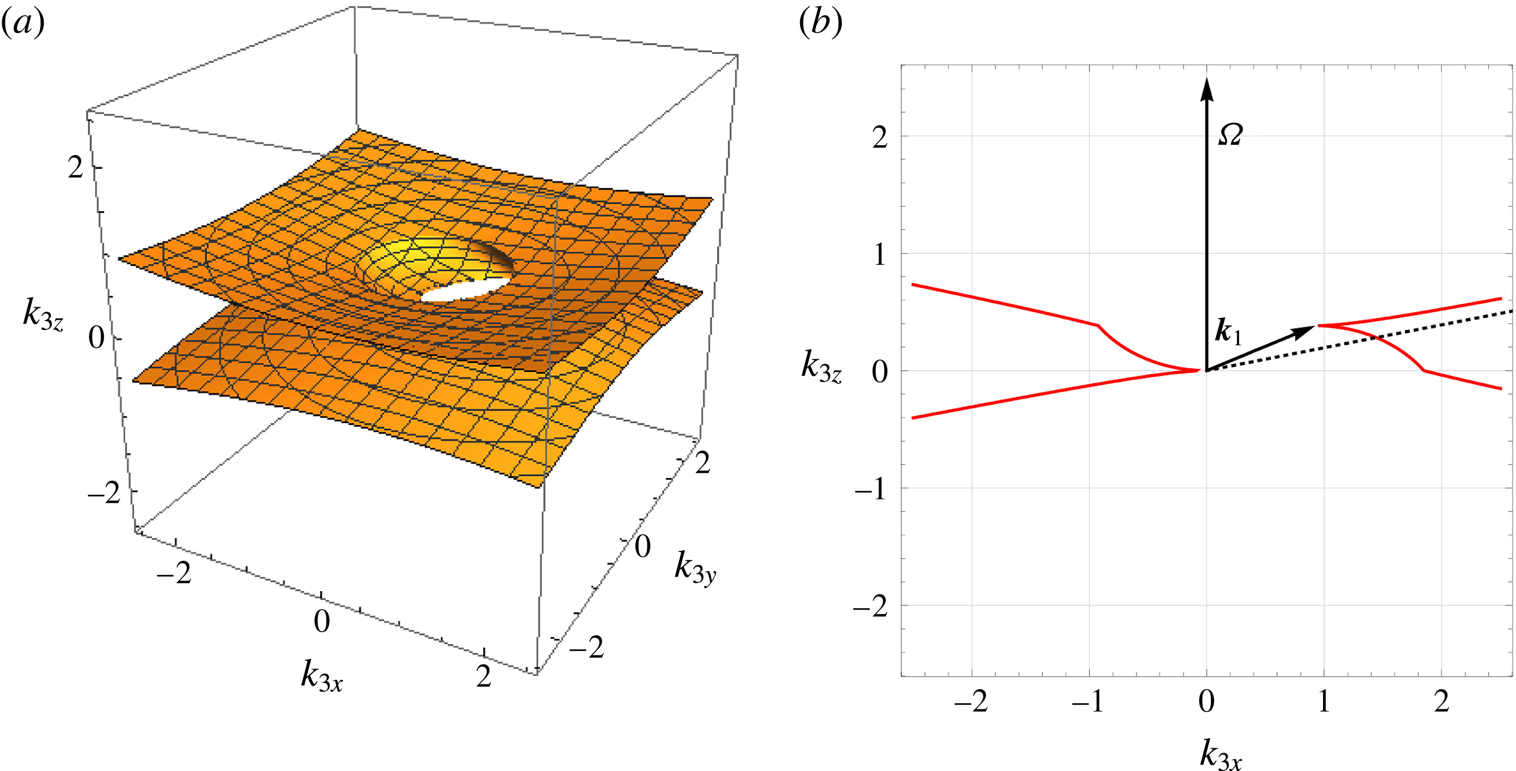
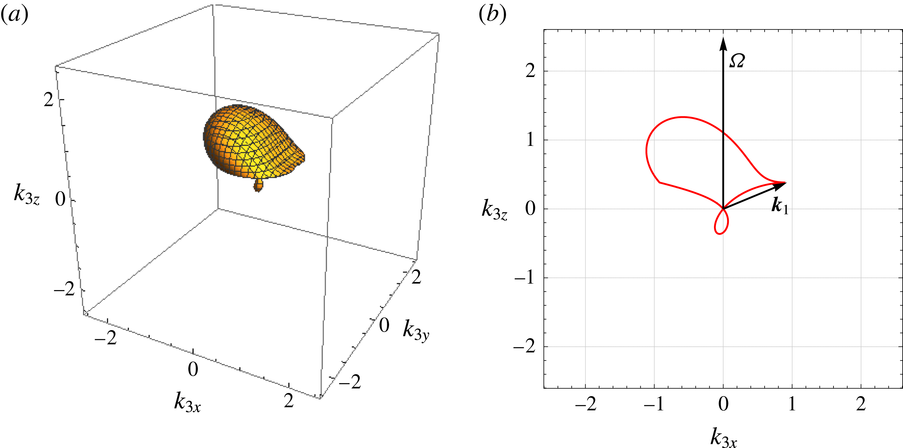
Since the expression (4.2) cannot be resolved explicitly, we find solutions numerically using ‘Wolfram Mathematica’. In figure 1 we present an example of a resonance surface and its two-dimensional cut in a specific direction – the so-called resonance curve. The energy of the primary wave $\boldsymbol{k}_{1}$ is always larger than the energy of the secondary waves $\boldsymbol{k}_{2}$ and $\boldsymbol{k}_{3}$ . Thus, according to the dispersion relation (1.1), the directions of the secondary waves are always closer to the $xy$ -plane than the direction of the vector $\boldsymbol{k}_{1}$ – see the figure 1(b).

Figure 1.

(a) The resonance surface of the wave vector $\boldsymbol{k}_{3}$ for the decay process $\boldsymbol{k}_{1}\rightarrow \boldsymbol{k}_{2}+\boldsymbol{k}_{3}$ . The primary wave vector $\boldsymbol{k}_{1}=(\sin (3\unicode[STIX]{x03C0}/8),0,\cos (3\unicode[STIX]{x03C0}/8))$ . (b) The cut of this surface (resonance curve) along the $k_{x}k_{z}$ -plane.

The resonance surface, having a non-trivial form with branches at $k\rightarrow \infty$ , formally allows decay into secondary waves of arbitrary small wavelength (in the experiment, this is obviously limited by the dissipation rate). We find the following asymptotics for the infinite branches assuming (4.2) $k_{3}\rightarrow \infty$ :

(4.3) $$\begin{eqnarray}\frac{|k_{1}\cos \unicode[STIX]{x1D703}_{1}|}{2}=\frac{|k_{3z}|}{\sqrt{k_{3x}^{2}+k_{3y}^{2}+k_{3z}^{2}}},\end{eqnarray}$$

(see figure 1 b). In addition, we study the process of wave confluence

(4.4) $$\begin{eqnarray}\boldsymbol{k}_{1}+\boldsymbol{k}_{2}\rightarrow \boldsymbol{k}_{3}.\end{eqnarray}$$

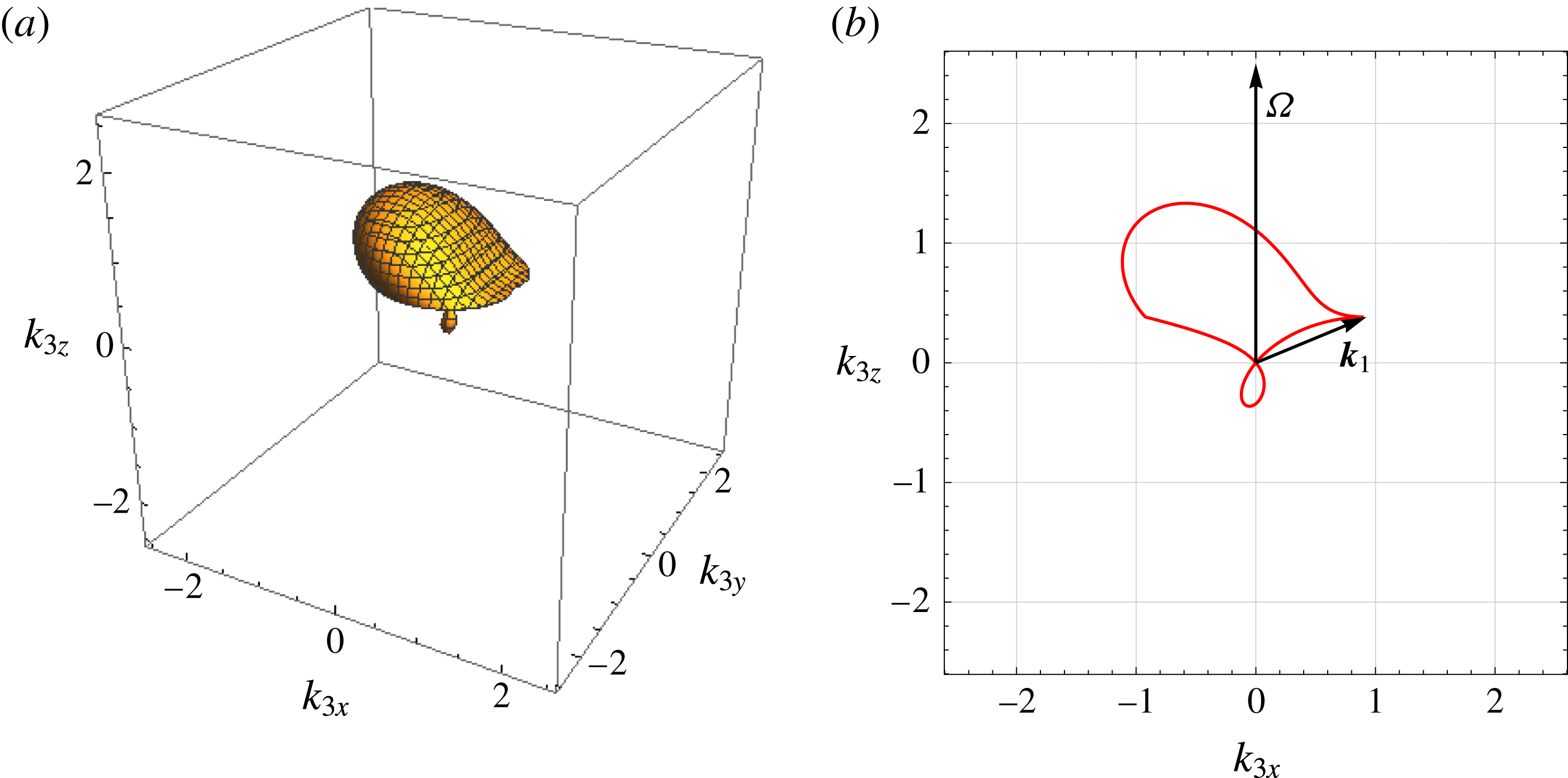
In figure 2, we plot the corresponding resonance surface that is obtained similarly to the equation (4.2) relation for the process (4.4). The confluence resonance surface remains finite in $\boldsymbol{k}$ -space and grows in size when $\unicode[STIX]{x1D703}_{1}$ tends to $\unicode[STIX]{x03C0}/2$ .

Figure 2.

(a) The resonance surface of wave vector $\boldsymbol{k}_{3}$ for the confluence process $\boldsymbol{k}_{1}+\boldsymbol{k}_{2}\rightarrow \boldsymbol{k}_{3}$ . The primary wave vector $\boldsymbol{k}_{1}=(\sin (3\unicode[STIX]{x03C0}/8),0,\cos (3\unicode[STIX]{x03C0}/8))$ . (b) The cut of this surface (resonance curve) along the $k_{x}k_{z}$ -plane.

Figure 3.

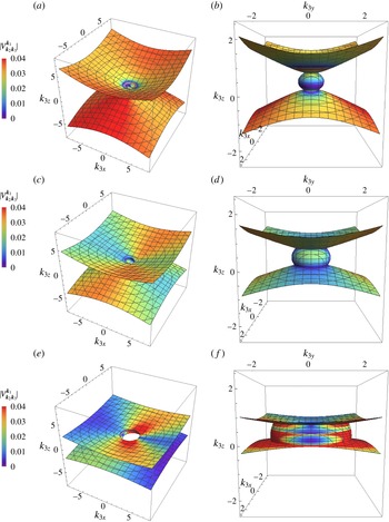
The resonance surface of the wave vector $\boldsymbol{k}_{3}$ for the decay process $\boldsymbol{k}_{1}\rightarrow \boldsymbol{k}_{2}+\boldsymbol{k}_{3}$ , coloured according to the value of $|V_{\boldsymbol{k}_{2}\boldsymbol{k}_{3}}^{\boldsymbol{k}_{1}}|$ . (a,b) $\boldsymbol{k}_{1}=(\sin (3\unicode[STIX]{x03C0}/8),0,\cos (3\unicode[STIX]{x03C0}/8))$ , (c,d) $\boldsymbol{k}_{1}=(\sin (\unicode[STIX]{x03C0}/4),0,\cos (\unicode[STIX]{x03C0}/4))$ , (e,f) $\boldsymbol{k}_{1}=(\sin (\unicode[STIX]{x03C0}/8),0,\cos (\unicode[STIX]{x03C0}/8))$ . (a,c,e) and (b,d,f) Show the same surface at different scales and from different view points.

Figure 4.

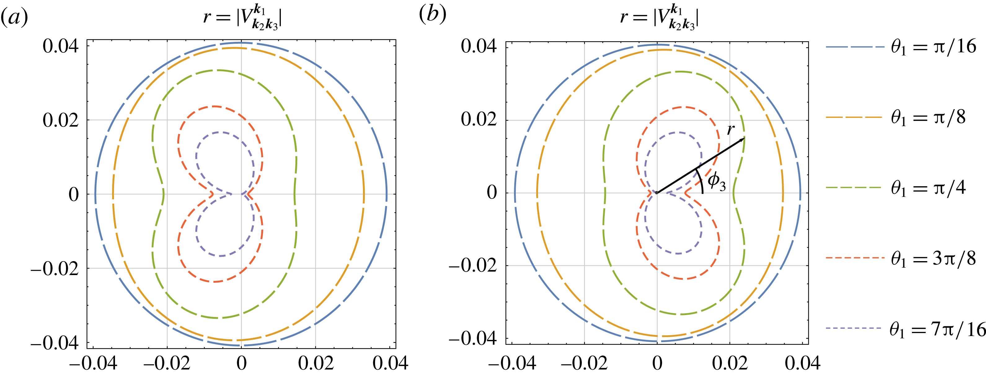
The polar diagram for the short-wave asymptotics (5.5) of the amplitude $|V_{\boldsymbol{k}_{2}\boldsymbol{k}_{3}}^{\boldsymbol{k}_{1}}(\unicode[STIX]{x1D711}_{3})|$ on the resonance surface. The primary wave vector $\boldsymbol{k}_{1}=(\sin \unicode[STIX]{x1D703}_{1},0,\cos \unicode[STIX]{x1D703}_{1})$ . The amplitude at a certain angle $\unicode[STIX]{x1D711}_{3}$ is given by the length of the corresponding radius vector. (a) Corresponds to the lower branch of the resonance surface; (b) corresponds to the upper branch.

5 Decay instability

The decay process $\boldsymbol{k}_{1}\rightarrow \boldsymbol{k}_{2}+\boldsymbol{k}_{3}$ , which is allowed by the dispersion law (1.1), leads to instability of the inertial waves with respect to weak perturbations. In the general weakly nonlinear wave system with the decay-type dispersion law, the perturbations grow exponentially in the initial (linear) stage of this decay instability (see, e.g. Zakharov et al. Reference Zakharov, L’vov and Falkovich1992). Consider at $t=0$ the primary wave of amplitude $A_{\boldsymbol{k}_{1}}$ and secondary waves of small amplitudes $A_{\boldsymbol{k}_{2}}$ and $A_{\boldsymbol{k}_{3}}$ playing the role of perturbations: $A_{\boldsymbol{k}_{1}}(0)\gg \max (|A_{\boldsymbol{k}_{2}}(0)|,|A_{\boldsymbol{k}_{3}}(0)|)$ . Then, according to the well-known theory (see, e.g. § 1 in L’vov (Reference L’vov1994)), the amplitudes of the secondary waves grow with time $t$ as

(5.1) $$\begin{eqnarray}A_{\boldsymbol{k}_{2,3}}(t)=A_{\boldsymbol{k}_{2,3}}(0)\exp (\unicode[STIX]{x1D706}t),\end{eqnarray}$$

during the linear stage of the decay instability (meanwhile $A_{\boldsymbol{k}_{1}}\sim$ const.). Here,

(5.2) $$\begin{eqnarray}\unicode[STIX]{x1D706}=\frac{\text{i}\unicode[STIX]{x0394}\unicode[STIX]{x1D714}_{\boldsymbol{k}}}{2}+\unicode[STIX]{x1D6FE},\quad \unicode[STIX]{x0394}\unicode[STIX]{x1D714}_{\boldsymbol{k}}\equiv \unicode[STIX]{x1D714}_{\boldsymbol{k}_{1}}-\unicode[STIX]{x1D714}_{\boldsymbol{k}_{2}}-\unicode[STIX]{x1D714}_{\boldsymbol{k}_{3}}.\end{eqnarray}$$

The growth rate of the decay instability

(5.3) $$\begin{eqnarray}\unicode[STIX]{x1D6FE}=\sqrt{4|V_{\boldsymbol{k}_{2}\boldsymbol{ k}_{3}}^{\boldsymbol{ k}_{1}}|^{2}|A_{\boldsymbol{k}_{1}}|^{2}-\frac{\unicode[STIX]{x0394}\unicode[STIX]{x1D714}_{\boldsymbol{k}}^{2}}{4}},\end{eqnarray}$$

is localized in the layer (in $\boldsymbol{k}$ -space) of thickness $8|V_{\boldsymbol{k}_{2}\boldsymbol{k}_{3}}^{\boldsymbol{k}_{1}}|^{2}|A_{k}(0)|^{2}$ near the resonance surface $\unicode[STIX]{x0394}\unicode[STIX]{x1D714}_{\boldsymbol{k}}=0$  (4.2), where it reaches the maximum value:

(5.4) $$\begin{eqnarray}\unicode[STIX]{x1D6FE}_{max}=2|V_{\boldsymbol{k}_{2}\boldsymbol{k}_{3}}^{\boldsymbol{ k}_{1}}||A_{k}(0)|.\end{eqnarray}$$

In this section, we study the absolute value of the three-wave decay amplitude $|V_{\boldsymbol{k}_{2}\boldsymbol{k}_{3}}^{\boldsymbol{k}_{1}}|$  (3.27) at the resonance surface (4.2), which is sufficient to describe the main features of the instability growth rate behaviour. In figure 3, we present the typical examples of a resonance surface, coloured according to the value of $|V_{\boldsymbol{k}_{2}\boldsymbol{k}_{3}}^{\boldsymbol{k}_{1}}|$ .

We find that the decay amplitude has a non-zero value on the infinite branches of the resonance surface (see the figure 3). Thus, decay instability appears even for short-wave perturbations up to the dissipative threshold. We calculate the short-wave asymptotic expression of the decay amplitude $V_{\boldsymbol{k}_{2}\boldsymbol{k}_{3}}^{\boldsymbol{k}_{1}}$ on the upper infinite branch of the resonance surface (i.e. at $k_{3}\rightarrow \infty$ and $\unicode[STIX]{x1D714}_{\boldsymbol{k}_{1}}=\unicode[STIX]{x1D714}_{\boldsymbol{k}_{2}}+\unicode[STIX]{x1D714}_{\boldsymbol{k}_{3}}$ ) using equations (3.27), (4.1), (4.2), (4.3):

(5.5) $$\begin{eqnarray}\displaystyle & & \displaystyle V_{\boldsymbol{k}_{2}\boldsymbol{k}_{3}}^{\boldsymbol{k}_{1}}(\unicode[STIX]{x1D711}_{3})\approx \frac{\text{i}\sqrt{2\unicode[STIX]{x1D6FA}}}{(2\unicode[STIX]{x03C0})^{3/2}}\left\{-\frac{1}{4}\sqrt{\frac{\unicode[STIX]{x1D714}_{\boldsymbol{k}_{1}}}{\unicode[STIX]{x1D6FA}}}\sin \unicode[STIX]{x1D711}_{3}\cos \unicode[STIX]{x1D711}_{3}\sin \unicode[STIX]{x1D703}_{1}\left(1+\frac{5}{16}\frac{\unicode[STIX]{x1D714}_{\boldsymbol{k}_{1}}^{2}}{\unicode[STIX]{x1D6FA}^{2}}\right)\right.\nonumber\\ \displaystyle & & \displaystyle \quad -\,\frac{1}{2}\sqrt{\frac{\unicode[STIX]{x1D6FA}}{\unicode[STIX]{x1D714}_{\boldsymbol{k}_{1}}}}\frac{\sin \unicode[STIX]{x1D711}_{3}\cos \unicode[STIX]{x1D703}_{1}}{\sqrt{1-\unicode[STIX]{x1D714}_{\boldsymbol{k}_{1}}^{2}/16\unicode[STIX]{x1D6FA}^{2}}}\left(1-\frac{11}{16}\frac{\unicode[STIX]{x1D714}_{\boldsymbol{k}_{1}}^{2}}{\unicode[STIX]{x1D6FA}^{2}}+\frac{5}{128}\frac{\unicode[STIX]{x1D714}_{\boldsymbol{k}_{1}}^{4}}{\unicode[STIX]{x1D6FA}^{4}}\right)\nonumber\\ \displaystyle & & \displaystyle \quad -\,\frac{3\text{i}}{16}\left(\frac{\unicode[STIX]{x1D714}_{\boldsymbol{k}_{1}}}{\unicode[STIX]{x1D6FA}}\right)^{3/2}\sqrt{1-\frac{\unicode[STIX]{x1D714}_{\boldsymbol{k}_{1}}^{2}}{4\unicode[STIX]{x1D6FA}^{2}}}\sin ^{2}\unicode[STIX]{x1D711}_{3}+\frac{\text{i}}{2}\left(\frac{\unicode[STIX]{x1D714}_{\boldsymbol{k}_{1}}}{4\unicode[STIX]{x1D6FA}}\sin \unicode[STIX]{x1D703}_{1}\cos \unicode[STIX]{x1D711}_{3}-\sqrt{1-\frac{\unicode[STIX]{x1D714}_{\boldsymbol{k}_{1}}^{2}}{16\unicode[STIX]{x1D6FA}^{2}}}\cos \unicode[STIX]{x1D703}_{1}\right)\nonumber\\ \displaystyle & & \displaystyle \quad \times \left[\frac{3}{2}\sqrt{\frac{\unicode[STIX]{x1D714}_{\boldsymbol{k}_{1}}}{\unicode[STIX]{x1D6FA}}}\cos \unicode[STIX]{x1D711}_{3}-\sqrt{\frac{\unicode[STIX]{x1D6FA}}{\unicode[STIX]{x1D714}_{\boldsymbol{ k}_{1}}}\left(1-\frac{\unicode[STIX]{x1D714}_{\boldsymbol{k}_{1}}^{2}}{16\unicode[STIX]{x1D6FA}^{2}}\right)}\right.\nonumber\\ \displaystyle & & \displaystyle \quad \times \left.\left.\left(\frac{\unicode[STIX]{x1D714}_{\boldsymbol{k}_{1}}}{\unicode[STIX]{x1D6FA}}\sqrt{1-\frac{\unicode[STIX]{x1D714}_{\boldsymbol{k}_{1}}^{2}}{16\unicode[STIX]{x1D6FA}^{2}}}\cos \unicode[STIX]{x1D711}_{3}-\cos \unicode[STIX]{x1D703}_{1}\sin \unicode[STIX]{x1D703}_{1}\right)\right]\right\}.\end{eqnarray}$$

The short-wave asymptotics for the lower infinite branch of the resonance surface can be obtained from the expression (5.5) by the transformation $\unicode[STIX]{x1D711}_{3}\rightarrow \unicode[STIX]{x1D711}_{3}+\unicode[STIX]{x03C0}$ . In figure 4, we present the angular dependence of the asymptotic (5.5) for different values of the primary vector $\boldsymbol{k}_{1}$ . As one can see, the growth rate has asymptotically constant value, depending only on polar angle. This means that the discussed problem is well posed even in the theory without dissipation. The short-wave asymptotic is almost isotropic around the rotational axes $\unicode[STIX]{x1D734}\Vert \widehat{\boldsymbol{z}}$ when the direction of $\boldsymbol{k}_{1}$ is close to the $xy$ -plane (i.e. the energy of the primary wave is low). In the opposite limit – when the primary wave propagates almost parallel to the rotational axes – the short-wave asymptotic is anisotropic with maxima near $\unicode[STIX]{x1D711}_{3}=\unicode[STIX]{x03C0}/4;3\unicode[STIX]{x03C0}/4$ , but its characteristic amplitude decreases.

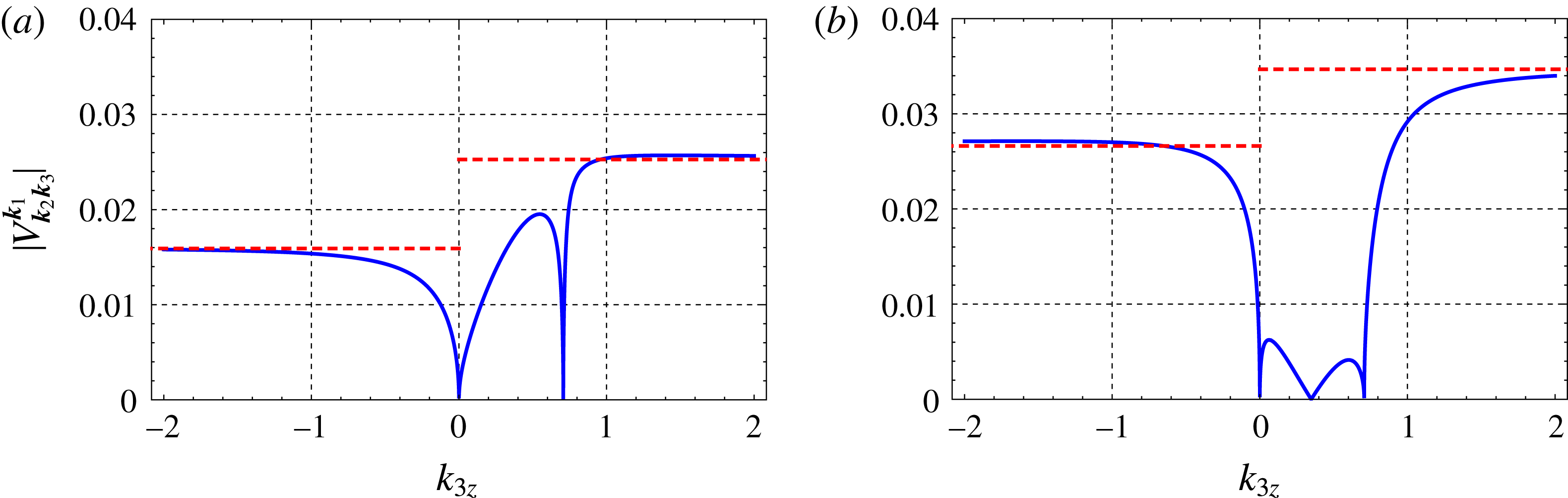
Figure 1 demonstrates that the right ( $k_{3x}>0$ ) and left ( $k_{3x}<0$ ) parts of the decay resonance curve can be represented as a single-valued function of $k_{3z}$ . This enables us to plot the values of the amplitude (3.27) on the resonance curve as a function of one variable – see figure 5.

Figure 5.

The behaviour of the amplitude $|V_{\boldsymbol{k}_{2}\boldsymbol{k}_{3}}^{\boldsymbol{k}_{1}}|$ (blue solid lines) on the resonance curve as a function of $k_{3z}$ . The primary wave vector $\boldsymbol{k}_{1}=(\sin (\unicode[STIX]{x03C0}/4),0,\cos (\unicode[STIX]{x03C0}/4))$ . (a) The resonance curve at $\unicode[STIX]{x1D711}_{1}=\unicode[STIX]{x03C0}/8$ . The amplitude has a local maximum at the middle branch of the resonance curve and a minimum at the point where one branch of the resonance curve changes to another; then, it approaches to the short-wave asymptotic (5.5) (red dotted lines). (b) The resonance curve at $\unicode[STIX]{x1D711}_{1}=3\unicode[STIX]{x03C0}/8$ . The growth rate has two local maxima and one minimum in the middle branch of the resonance curve. Again, the short-wave asymptotic (5.5) is represented by the red dotted curve.

As we will discuss in the next section, the anisotropic case, when $k_{z}\ll k_{\bot }$ , plays a central role in the statistical behaviour of inertial waves. Such waves, propagating predominantly in the $\boldsymbol{k}_{\bot }$ -direction, have low energy and frequency, according to the dispersion law (1.1). Here, we find the following asymptotics for the amplitude $V_{\boldsymbol{k}_{2}\boldsymbol{k}_{3}}^{\boldsymbol{k}_{1}}$ in this small frequency limit (i.e. at $k_{z}\ll k_{\bot }$ ):

(5.6) $$\begin{eqnarray}\displaystyle V_{\boldsymbol{k}_{2}\boldsymbol{k}_{3}}^{\boldsymbol{k}_{1}} & {\approx} & \displaystyle \frac{\text{i}}{16\unicode[STIX]{x03C0}^{3/2}}\frac{S_{\boldsymbol{k}_{2}\boldsymbol{k}_{3}}}{k_{1\bot }k_{2\bot }k_{3\bot }\sqrt{\unicode[STIX]{x1D714}_{\boldsymbol{k}_{1}}\unicode[STIX]{x1D714}_{\boldsymbol{k}_{2}}\unicode[STIX]{x1D714}_{\boldsymbol{k}_{3}}}}\nonumber\\ \displaystyle & & \displaystyle \times \,[\unicode[STIX]{x1D714}_{\boldsymbol{k}_{1}}^{2}(k_{3\bot }^{2}-k_{2\bot }^{2})+\unicode[STIX]{x1D714}_{\boldsymbol{k}_{2}}^{2}(k_{1\bot }^{2}-k_{3\bot }^{2})-\unicode[STIX]{x1D714}_{\boldsymbol{k}_{3}}^{2}(k_{1\bot }^{2}-k_{2\bot }^{2})].\end{eqnarray}$$

The asymptotic (5.6), as a function of $\boldsymbol{k}_{3}$ , is valid not only in the short-wave limit but for any point of the small-frequency resonance surface. 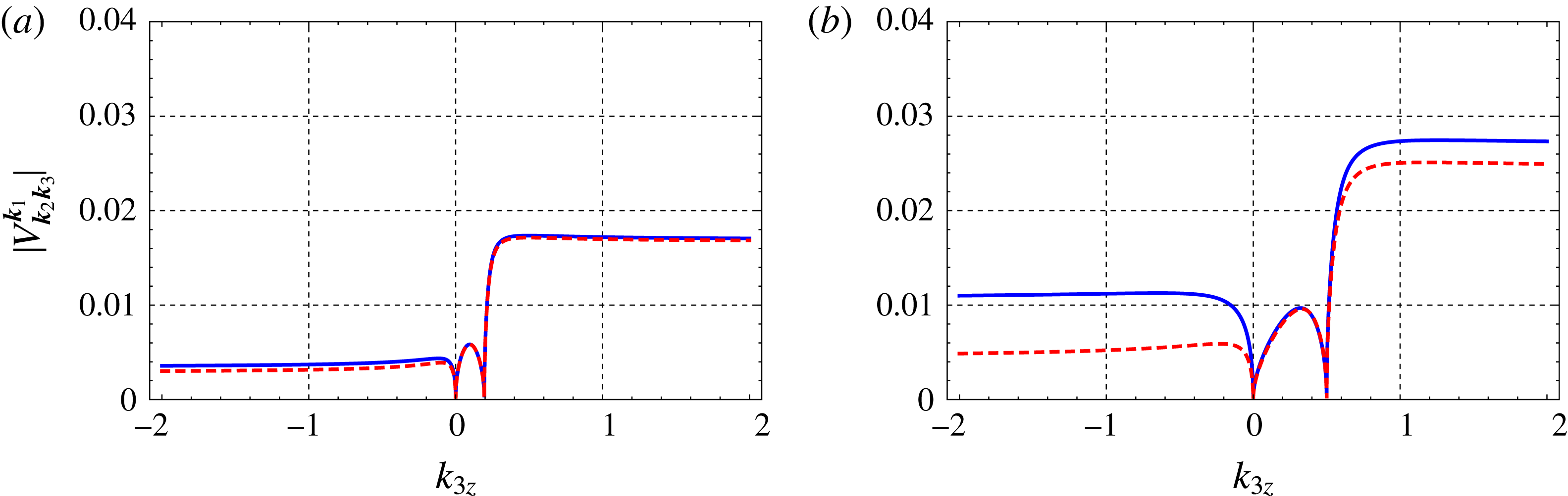As was found by Bayly (Reference Bayly1986), the addition of weak ellipticity to the circular flow of the fluid leads to excitation of parametric inertial waves with maximum growth rate at angles $\unicode[STIX]{x1D703}_{p}$ , satisfying the condition $|\text{cos}\,\unicode[STIX]{x1D703}_{p}|=1/2$ (see also the conclusion section). In figure 6 we demonstrate how the small-frequency asymptotic (5.6) works at small frequencies and in the especially important case where $\unicode[STIX]{x1D703}=\unicode[STIX]{x1D703}_{p}=\unicode[STIX]{x03C0}/3$ . We find that in the first case, the asymptotics (5.6) perfectly describe the three-wave interaction processes on the whole resonance surface and can be used instead of the cumbersome exact expression (3.27). Meanwhile, for the latter case, the small-frequency asymptotics (5.6) work well only in the middle branch of the resonance surface.

Figure 6.

Comparison of the exact amplitude $|V_{\boldsymbol{k}_{2}\boldsymbol{k}_{3}}^{\boldsymbol{k}_{1}}|$ given by (3.27) (blue solid lines) and its small-frequency asymptotics given by (5.6) (red dashed lines). The resonance curves are presented for $\unicode[STIX]{x1D711}_{1}=\unicode[STIX]{x03C0}/4$ . (a) The primary wave vector $\boldsymbol{k}_{1}=(\sin (7\unicode[STIX]{x03C0}/16),0,\cos (7\unicode[STIX]{x03C0}/16))$ . (b) $\boldsymbol{k}_{1}=(\sin \unicode[STIX]{x1D703}_{p},0,\cos \unicode[STIX]{x1D703}_{p})$ .

The presented study of the instability growth rate is in agreement with the results of Bordes et al. (Reference Bordes, Moisy, Dauxois and Cortet2012), where the particular two-dimensional case (i.e. when $\boldsymbol{k}_{1}$ , $\boldsymbol{k}_{2}$ and $\boldsymbol{k}_{3}$ lie in one plane) was studied experimentally and theoretically (using the helical modes decomposition approach). In particular, the non-zero values of the growth rate in the short-wave limit were also studied. Here, we provide a more detailed description of the growth rate in the whole $\boldsymbol{k}$ -space, which we believe will be useful for the future experimental and numerical works devoted to the three-wave interactions of inertial waves.

6 Turbulent cascade of the inertial waves

Secondary waves, created as a result of the decay instability of the primary waves, are also unstable with respect to the same process (1.3a ). Thus, one can expect that this multi-level decay instability will result in the formation of some type of energy cascade from the large scale toward the small scale, as in usual homogeneous turbulence. The energy spectrum in the inertial range (i.e. at intermediate scale) of the cascade can be found from the well-known kinetic equation, which for three-wave processes has the following form:

(6.1) $$\begin{eqnarray}\displaystyle \frac{\unicode[STIX]{x2202}n(\boldsymbol{k}_{1},t)}{\unicode[STIX]{x2202}t} & = & \displaystyle \unicode[STIX]{x03C0}\int [\!|V_{\boldsymbol{k}_{2}\boldsymbol{k}_{3}}^{\boldsymbol{k}_{1}}|^{2}N_{\boldsymbol{ k}_{2}\boldsymbol{k}_{3}}^{\boldsymbol{k}_{1}}\unicode[STIX]{x1D6FF}_{\boldsymbol{k}_{1}-\boldsymbol{k}_{2}-\boldsymbol{k}_{3}}\unicode[STIX]{x1D6FF}_{\unicode[STIX]{x1D714}_{\boldsymbol{k}_{1}}-\unicode[STIX]{x1D714}_{\boldsymbol{k}_{2}}-\unicode[STIX]{x1D714}_{\boldsymbol{k}_{3}}}\nonumber\\ \displaystyle & & \displaystyle +\,2|V_{\boldsymbol{k}_{1}\boldsymbol{k}_{3}}^{\boldsymbol{k}_{2}}|^{2}N_{\boldsymbol{ k}_{1}\boldsymbol{k}_{3}}^{\boldsymbol{k}_{2}}\unicode[STIX]{x1D6FF}_{\boldsymbol{k}_{2}-\boldsymbol{k}_{1}-\boldsymbol{k}_{3}}\unicode[STIX]{x1D6FF}_{\unicode[STIX]{x1D714}_{\boldsymbol{k}_{2}}-\unicode[STIX]{x1D714}_{\boldsymbol{k}_{1}}-\unicode[STIX]{x1D714}_{\boldsymbol{k}_{3}}}\! ]\,\text{d}\boldsymbol{k}_{2}\,\text{d}\boldsymbol{k}_{3}.\end{eqnarray}$$

Here

(6.2) $$\begin{eqnarray}N_{\boldsymbol{k}_{2}\boldsymbol{k}_{3}}^{\boldsymbol{ k}_{1}}=n_{\boldsymbol{k}_{2}}n_{\boldsymbol{k}_{3}}-n_{\boldsymbol{k}_{1}}(n_{\boldsymbol{k}_{2}}+n_{\boldsymbol{k}_{3}}),\end{eqnarray}$$

and $n_{\boldsymbol{k}}$ is the wave density in $\boldsymbol{k}$ -space. The solution of the kinetic (6.1) can be found only in particular cases, when both matrix elements and the eigen-frequency have some scaling properties (see the book Zakharov et al. (Reference Zakharov, L’vov and Falkovich1992)). Unfortunately, this is not the case for inertial waves in rotating fluid.

However, it is well established that the statistical behaviour of inertial waves in rapidly rotating fluids is highly anisotropic (see, for instance, Galtier (Reference Galtier2003), Sen et al. (Reference Sen, Mininni, Rosenberg and Pouquet2012) or the book of Nazarenko (Reference Nazarenko2011) and references therein). The dispersion law (1.1) leads to the formation of an energy cascade predominantly in the $\boldsymbol{k}_{\bot }$ direction, when the wave frequencies are small and our simple asymptotic (5.6) is valid. Under this approximation, the dispersion law and interaction amplitude become scale invariant with respect to scaling of $k_{z}$ and $k_{\bot }$ :

(6.3a,b ) $$\begin{eqnarray}\unicode[STIX]{x1D714}_{\boldsymbol{k}}=2\unicode[STIX]{x1D6FA}\frac{k_{z}}{k_{\bot }},\quad V_{\boldsymbol{k}_{1}\boldsymbol{k}_{3}}^{\boldsymbol{ k}_{2}}\sim \sqrt{\unicode[STIX]{x1D6FA}k_{z}k_{\bot }}.\end{eqnarray}$$

As was discovered by  Kuznetsov (Reference Kuznetsov1972), in such cases one can find anisotropic solutions of the kinetic equation. The result is that for the scaling, given by (6.3), stationary solutions of the kinetic equation, corresponding to the constant densities of the energy flux ${\mathcal{P}}_{1}$ and momentum flux ${\mathcal{P}}_{2}$ along the $\widehat{\boldsymbol{z}}$ direction, can be found as

(6.4a,b ) $$\begin{eqnarray}\displaystyle {\mathcal{E}}_{1}(\boldsymbol{k})\equiv {\mathcal{P}}_{1}^{1/2}k_{z}^{-1/2}k_{\bot }^{-7/2},\quad {\mathcal{E}}_{2}(\boldsymbol{k})\equiv {\mathcal{P}}_{2}^{1/2}k_{z}^{-1/2}k_{\bot }^{-4}. & & \displaystyle\end{eqnarray}$$

These anisotropic weak turbulent energy spectra were first identified by Galtier (Reference Galtier2003) using the helical modes decomposition approach. Here, we present spectra not averaged by the azimuth angle $\unicode[STIX]{x1D711}$ , which explains the difference in the power laws of (6.4) and the paper of Galtier (Reference Galtier2003).