1. Introduction
Over the last years, the development of augmented reality (AR) systems triggered researchers to investigate new applications for this technology. Within the maritime domain, it may be an intuitive technique to display spatial information in comparison with traditional methods. We are particularly interested in the application of AR systems for the assistance of maritime navigation. Technically, AR has the potential to improve decision-making while enhancing navigational awareness (Hong et al., Reference Hong, Andrew and Kenny2015). Examples of AR scenes combining pertinent virtual elements to potentially assist operators in maritime navigation can be found in Leite et al. (Reference Leite, Sinohara, Maruyama and Tannuri2022).
Some researchers pursued methodologies that enable investigating AR in maritime scenarios independently from the maturation of this technology. A typical approach investigates AR usability by simulating scenarios without sensor errors that would ultimately affect the performance of any AR system. Wisernig et al. (Reference Wisernig, Sadhu, Zilinski, Wyvill, Albu and Hoeberechts2015) propose an AR system prototype based on simulated real-time data. Evaluations with experienced sailors were performed to address which and how information should be displayed. The reported acceptance was very positive. Butkiewicz (Reference Butkiewicz2017) proposed an immersive virtual reality simulator to perform visualisation and interaction research. Usability issues such as information overload and occlusion were identified, and potential mitigation techniques were discussed. The author concludes that AR has a great potential to support safe marine navigation in the near future. Laera et al. (Reference Laera, Fiorentino, Evangelista, Boccaccio, Manghisi, Gabbard, Gattullo, Uva and Foglia2021) implemented a virtual simulator of a sailboat in a marine environment to evaluate the effectiveness of wind representation in an AR interface. A test scenario was presented to 75 sailors who afterwards answered an online questionnaire regarding their experience. The questionnaire revealed a real interest in the use of AR for sailor boat activities.
Recent systematic literature reviews (Laera et al., Reference Laera, Fiorentino, Evangelista, Boccaccio, Manghisi, Gabbard, Gattullo, Uva and Foglia2021; Van Den Oever et al., Reference Van Den Oever, Fjeld and Sætrevik2023) reports that most of the prototypes proposed in the literature are still in early development. Among studies focused on field tests from implementations of AR technology, performance issues are often qualitatively reported without means of quantification, such as the incorrect projection of virtual elements. For example, during the development of an advanced navigation aids system based on AR, Jaeyong et al. (Reference Jaeyong, Park and Kwon2016) briefly reported cases with errors in virtual projections. Another study focused on the exploration of designs of AR systems for ship bridges in artic waters (Frydenberg et al., Reference Frydenberg, Nordby and Eikenes2018) reported problems with performing a consistent environmental tracking alongside movements of the system. In another study designed to evaluate AR as a skipper’s navigator (Hertel et al., Reference Hertel, Schmidt, Briede, Anders, Thies and Steinicke2023), multiple participants experienced unexpected behaviour, such as virtual elements disappearing at times, or jumping or being tilted.
Despite such issues, there are already a few commercial AR solutions available in the market such as Furuno’s Envision AR (Furuno, 2024) and Raymarine’s ClearCruise AR (Raymarine, 2024). Both systems are monitor-based and their accuracy is not clearly defined in quantitative terms. A monitor-based setup, commonly known as monitor-augmented reality (MAR), uses a camera to observe the environment and a screen to display the scene augmented with virtual elements. This setup contrasts with another type of architecture based on head-mounted displays (HMD-AR), in which a device is mounted on the head of the viewer. Such HMD devices may be based on video, where a camera streams its recording to attached displays at the front of the viewer, or on a see-through glass, where the user views the scene directly. HMD-AR architectures offer greater immersion and are generally preferred over MAR setups, which are simpler to deploy and are currently the main architecture for maritime navigation assistance.
In this context, we propose a theoretical model to describe the error between a virtual projection and its corresponding real observation that arises from uncertainties in the parameters from a MAR system. This enables the determination of confidence bounds for each projection, which enables users to understand the validity of each virtual projected information and act accordingly to the quality of the information. The proposed model also enables the comparison between different potential MAR setups and the definition of minimum precision requirements given a desired maximum projection error. The model is validated with numerical simulations and a navigation experiment. Therefore, our contribution enables preliminary assessments regarding how precisely MAR parameters need to be determined in view of a simple yet useful error quantity. Such assessments may be useful for the robust development of maritime navigational assistance by AR systems. While the proposed model can be adapted to describe projection errors in any AR system with camera-fed displays, it is not applicable to HMD-AR systems using optical see-through displays.
2. Background
2.1. Augmented reality systems
Augmented reality (AR) may be defined as systems that displays three-dimensional virtual objects in an environment with interactivity in real-time (Azuma, Reference Azuma1997). Typically, each virtual element is represented with a model that is specified by its position and orientation in an environment frame. The viewer position and orientation is estimated by a tracker component in real-time. The virtual object position and orientation at the camera frame is computed and its visual representation is rendered. Note that errors in the determination of the viewer position and orientation yields misplaced virtual objects. This alignment between the virtual and real environment is one of the fundamental problems of AR and is typically referred to as geometric registration. Thus, throughout the development of any AR system, it is interesting to ensure that the geometric registration is fulfilled with sufficient accuracy.
There are mainly two classes of AR displays: head-mounted displays (HMDs) and monitor-based displays. Head-mounted displays are equipment worn by users that provide a stereographic view of virtual objects in the scene through two simultaneous projections, one for each eye of the viewer. An example of a head-mounted display is the Microsoft Hololens 2 (Microsoft, 2024). Monitor-based displays are built with cameras to observe the environment and screens to display the scene. The simplest monitor-based configuration uses a camera and a fixed monitor screen to display its video stream. The camera position and orientation in the environment is tracked, and virtual elements are rendered over the scene in real-time. An example of a possible monitor-based display architecture is presented in Figure 1.
Monitor-based AR architecture (Leite et al., Reference Leite, Sinohara, Maruyama and Tannuri2022) adapted from (Azuma, Reference Azuma1997).

Generally, HMDs are preferable to monitor-based displays as they provide higher levels of immersion. However, there are anatomical considerations regarding the human visual system that may trigger discomfort and potential health issues for users. Such symptoms are collective referred to as cybersickness and are still not fully explored and explained in the literature (Porcino et al., Reference Porcino, Trevisan and Clua2020; Hughes et al., Reference Hughes, Fidopiastis, Stanney, Bailey and Ruiz2020). Furthermore, this type of display is significantly more complex to be deployed than are monitor-based displays. From a tracking perspective, as the user is enabled to look freely in the environment, the tracker component from the system must be particularly robust. In addition, from a display perspective, modelling each virtual element projection involves the determination of two set of coordinates according to each eye of the viewer. Both must be carefully aligned, synchronised and calibrated to specific physical characteristics of viewers. These factors may explain the popularity of monitor-based displays over HMDs for maritime navigation assistance applications (Laera et al., Reference Laera, Fiorentino, Evangelista, Boccaccio, Manghisi, Gabbard, Gattullo, Uva and Foglia2021). This motivates the current work to focus on MARs.
2.2. Maritime AR systems
In a study to explore requirements for an AR assistant within maritime operations (Bräker et al., Reference Bräker, Osterbrink, Semmann and Wiesche2023), five core requirements have been proposed: (1) real-time overlay, (2) variety in displaying information, (3) multi-dimensional tracking, (4) collaboration and (5) interaction. The authors highlights that one of the biggest technical challenges is appropriate tracking of the vessel and the viewer at the environment. Note that for an AR system to assist in maritime navigation, it is critical that the virtual elements inserted into the scene are correctly positioned. Different tracking setups for AR systems within maritime domains have been proposed in the literature over the last years.
Morgère et al. (Reference Morgère, Diguet and Laurent2014) proposed a tracking setup by the integration of global navigation satellite systems (GNSS) with an inertial measurement unit (IMU). The camera position is mainly determined from GNSS measurements, and its orientation is determined by the IMU. This architecture is preferred as it does not rely on visibility conditions. The proposed integration algorithm is based on Kalman filters. Requirements regarding how accurate the IMU must be are not straightforwardly defined, which negatively impacts the reliability and reproducibility of the results. Lee et al. (Reference Lee, Lee, Nam and Wu2016) proposed a tracking setup by the integration of GNSS with an image-processing algorithm. The position of the camera and its heading (yaw angle) is determined from GNSS measurements, and the remaining orientation angles (roll and pitch angles) are determined by the relative position of the horizon in the image. In this setup, registration errors occur when the horizon is not visible or if the image-processing algorithm detection fails. Okazaki et al. (Reference Okazaki, Takaseki, Shoji and Matsubara2017) proposed an interesting setup with the integration of GNSS signals and a camera stabiliser. The camera orientation is kept constant by a control loop composed by an IMU and compensation motors. The vessel and camera position are estimated from GNSS measurements. Requirements regarding the stabilisation control loop are not directly defined, either.
Overall, the authors are still unclear about the most adequate tracking setups and their components requirements to ensure the geometric registration of AR systems in maritime environments. Therefore, a simple model is derived to describe the error between a virtual projection and its corresponding real observation. Henceforth, this error will be referred to as projection error. Note that it reflects the quality of the geometric registration for a particular AR system.
2.3. Related work
Most research that models AR errors to assess accuracy use marker-based tracking systems (Bauer et al., Reference Bauer2006; Coelho et al., Reference Coelho, Julier and Maclntyre2004; Davis et al., Reference Davis, Clarkson and Rolland2003; Freeman et al., Reference Freeman, Julier and Steed2007; Holloway, Reference Holloway1997). In this type of tracking, visible known features are used as reference points to determine the viewer position and orientation. Such tracking setups are suitable for indoor environments in which it is possible to arbitrarily insert reference marks at the scene. For AR applications within maritime domains, however, it is not possible to modify the environment with markers. Thus, most results obtained in these previous works are not directly applicable to the development of AR systems for maritime navigational assistance.
3. Methods
3.1. Projection error model for AR systems
Let
 $ {p}_{cQ}^{c}=[{p}_{cQ}^{cx},{p}_{cQ}^{cy},{p}_{cQ}^{cz}]$
be the position of a point
 $ Q$
described with coordinates at a camera frame
 $ c$
and
 $ [{u}_{Q},{v}_{Q}{]}^{T}$
be the corresponding projection at the image frame. The first axis
 $ {\overrightarrow{x}\!\!}_{c}$
of the camera frame is oriented from left to right, the second axis
 $ {\overrightarrow{y}\!\!}_{c}$
is oriented downwards and axis
 $ {\overrightarrow{z}\!\!}_{c}$
is forward oriented. A simple model for pinhole projection may be expressed as (Hartley and Zisserman, Reference Hartley and Zisserman2003):
 $$\left[ {\matrix{ {{u_Q}} \hfill \cr {} \hfill \cr {{v_Q}} \hfill \cr } } \right] = \left[ {\matrix{ {{f_u}{{p_{cQ}^{cx}} \over {p_{cQ}^{cz}}} + {u_c}} \hfill \cr {} \hfill \cr {{f_v}{{p_{cQ}^{cy}} \over {p_{cQ}^{cz}}} + {v_c}} \hfill \cr } } \right],$$
where
 $ {f}\!_{u}$
,
 $ {f}\!_{v}$
,
 $ {u}_{c}$
and
 $ {v}_{c}$
are intrisic parameters from the camera. There are several methods to estimate camera intrinsic parameters shown in Equation (1) (Kannala and Brandt, Reference Kannala and Brandt2006; Zhang, 2003). Implementations are available in the functions calibrateCamera and calibrateCameraExtended from the OpenCV library (Bradski, Reference Bradski2000).
Consider a point
 $ Q'$
being an estimation of real point
 $ Q$
with coordinates
 $ {p}_{cQ'}^{c}=[{p}_{cQ'}^{cx},{p}_{cQ'}^{cy},{p}_{cQ'}^{cz}]$
and let
 $ {\hat{f}\!}_{u}$
,
 $ {\hat{f}\!}_{v}$
,
 $ {\hat{u}}_{c}$
and
 $ {\hat{v}}_{c}$
be estimations for the camera intrinsic parameters. The estimation
 $ [{\hat{u}}_{Q'},{\hat{v}}_{Q'}{]}^{T}$
and corresponding error
 $ [\Delta {u}_{Q},\Delta {v}_{Q}{]}^{T}$
may be expressed as:
 $$\left[ {\matrix{ {{{\hat u}_{Q'}}} \hfill \cr {} \hfill \cr {{{\hat v}_{Q'}}} \hfill \cr } } \right] = \left[ {\matrix{ {{{\hat f}_u}{{p_{cQ'}^{cx}} \over {p_{cQ'}^{cz}}} + {{\hat u}_c}} \hfill \cr {} \hfill \cr {{{\hat f}_v}{{p_{cQ'}^{cy}} \over {p_{cQ'}^{cz}}} + {{\hat v}_c}} \hfill \cr } } \right] \Rightarrow \left[ {\matrix{ {{u_Q} - {{\hat u}_{Q'}}} \hfill \cr {} \hfill \cr {{v_Q} - {{\hat v}_{Q'}}} \hfill \cr } } \right] = \left[ {\matrix{ {{\Delta }{u_Q}} \hfill \cr {} \hfill \cr {{\Delta }{v_Q}} \hfill \cr } } \right],$$
 $$\left[ {\matrix{ {{\Delta }{u_Q}} \hfill \cr {{\Delta }{v_Q}} \hfill \cr } } \right] = \left[ {\matrix{ {{f_u}{{p_{cQ}^{cx}} \over {p_{cQ}^{cz}}} + {u_c} - {{\hat f}_u}{{p_{cQ'}^{cx}} \over {p_{cQ'}^{cz}}} - {{\hat u}_c}} \hfill \cr {} \hfill \cr {{f_v}{{p_{cQ}^{cy}} \over {p_{cQ}^{cz}}} + {v_c} - {{\hat f}_v}{{p_{cQ'}^{cy}} \over {p_{cQ'}^{cz}}} - {{\hat v}_c}} \hfill \cr } } \right] = \left[ {\matrix{ {{{{f_u}p_{cQ}^{cx}p_{cQ'}^{cz} - {{\hat f}_u}p_{cQ'}^{cx}p_{cQ}^{cz}} \over {p_{cQ}^{cz}p_{cQ'}^{cz}}} + \left( {{u_c} - {{\hat u}_c}} \right)} \hfill \cr {} \hfill \cr {{{{f_v}p_{cQ}^{cy}p_{cQ'}^{cz} - {{\hat f}_v}p_{cQ'}^{cy}p_{cQ}^{cz}} \over {p_{cQ}^{cz}p_{cQ'}^{cz}}} + \left( {{v_c} - {{\hat v}_c}} \right)} \hfill \cr } } \right].$$
Let
 $ \Delta {f}_{u}$
,
 $ \Delta {f}_{v}$
,
 $ \Delta {u}_{c}$
and
 $ \Delta {v}_{c}$
be the errors in the estimated intrinsic parameters with
 $ \Delta {p}_{cQ}^{cx}$
,
 $ \Delta {p}_{cQ}^{cy}$
,
 $ \Delta {p}_{cQ}^{cz}$
being the errors in the position of
 $ Q$
.
 $$\eqalign{ & {f_u} = {{\hat f}_u} + \Delta {f_u} = {{\hat f}_u}\left( {1 + {{\Delta {f_u}} \over {{{\hat f}_u}}}} \right)\;,{f_v} = {{\hat f}_v} + \Delta {f_v} = {{\hat f}_v}\left( {1 + {{\Delta {f_v}} \over {{{\hat f}_v}}}} \right) \cr & {u_c} = {{\hat u}_c} + \Delta {u_c},\;\;{v_c} = {{\hat v}_c} + \Delta {v_c} \cr & p_{cQ}^{cx} = p_{cQ'}^{cx} + {\Delta }p_{cQ}^{cx}\;\;,p_{cQ}^{cy} = p_{cQ'}^{cy} + {\Delta }p_{cQ}^{cy} \cr & p_{cQ}^{cz} = p_{cQ'}^{cz} + {\Delta }p_{cQ}^{cz} = p_{cQ'}^{cz}\left( {1 + {{{\Delta }p_{cQ}^{cz}} \over {p_{cQ'}^{cz}}}} \right). \cr} $$
Substituting into Equation (3) yields:
 $${\Delta }{u_Q} = {{\left( {1 + {{{\Delta }{f_u}} \over {{{\hat f}_u}}}} \right)} \over {\left( {1 + {{{\Delta }p_{cQ}^{cz}} \over {p_{cQ'}^{cz}}}} \right)}}{{{{\hat f}_u}} \over {p_{cQ'}^{cz}}}{\Delta }p_{cQ}^{cx} + {{p_{cQ'}^{cx}} \over {p_{cQ'}^{cz}\left( {1 + {{{\Delta }p_{cQ}^{cz}} \over {p_{cQ'}^{cz}}}} \right)}}{\Delta }{f_u} - {{{{\hat f}_u}p_{cQ'}^{cx}} \over {{{(p_{cQ'}^{cz})}^2}\left( {1 + {{{\Delta }p_{cQ}^{cz}} \over {p_{cQ'}^{cz}}}} \right)}}{\Delta }p_{cQ}^{cz} + {\Delta }{u_c},$$
 $${\Delta }{v_Q} = {{\left( {1 + {{{\Delta }{f_v}} \over {{{\hat f}_v}}}} \right)} \over {\left( {1 + {{{\Delta }p_{cQ}^{cz}} \over {p_{cQ'}^{cz}}}} \right)}}{{{{\hat f}_v}} \over {p_{cQ'}^{cz}}}{\Delta }p_{cQ}^{cy} + {{p_{cQ'}^{cy}} \over {p_{cQ'}^{cz}\left( {1 + {{{\Delta }p_{cQ}^{cz}} \over {p_{cQ'}^{cz}}}} \right)}}{\Delta }{f_v} - {{{{\hat f}_v}p_{cQ'}^{cy}} \over {{{(p_{cQ'}^{cz})}^2}\left( {1 + {{{\Delta }p_{cQ}^{cz}} \over {p_{cQ'}^{cz}}}} \right)}}{\Delta }p_{cQ}^{cz} + {\Delta }{v_c}.$$
Assuming that
 $ \Delta {p}_{cQ}^{cz} \ll {p}_{cQ'}^{cz}$
,
 $ \Delta {f}_{u} \ll {\hat{f}\!}_{u}$
and
 $ \Delta {f}_{v} \ll {\hat{f}\!}_{v}$
:
 $${\Delta }{u_Q} = {{{{\hat f}_u}} \over {p_{cQ'}^{cz}}}{\Delta }p_{cQ}^{cx} + {{p_{cQ'}^{cx}} \over {p_{cQ'}^{cz}}}{\Delta }{f_u} - {{{{\hat f}_u}p_{cQ'}^{cx}} \over {{{(p_{cQ'}^{cz})}^2}}}{\Delta }p_{cQ}^{cz} + {\Delta }{u_c},$$
 $${\Delta }{v_Q} = {{{{\hat f}_v}} \over {p_{cQ'}^{cz}}}{\Delta }p_{cQ}^{cy} + {{p_{cQ'}^{cy}} \over {p_{cQ'}^{cz}}}{\Delta }{f_v} - {{{{\hat f}_v}p_{cQ'}^{cy}} \over {{{(p_{cQ'}^{cz})}^2}}}{\Delta }p_{cQ}^{cz} + {\Delta }{v_c}.$$
Let
 $ \Delta \Pi _{cam}=[\Delta {f}_{u},\Delta {f}_{v},\Delta {u}_{c},\Delta {v}_{c}{]}^{T}$
and
 $ \Delta \Pi _{pos}=[\Delta {p}_{cQ}^{cx},\Delta {p}_{cQ}^{cy},\Delta {p}_{cQ}^{cz}{]}^{T}$
. Reorganising in a matricial form:
 $${\left[ {\matrix{ {\Delta {u_Q}\Delta {v_Q}} \hfill \cr } } \right]^T} \approx {H_I}\Delta {\Pi _{cam}} + {H_P}\Delta {\Pi _{pos}},$$
 $$\left[ {\matrix{ {\Delta {u_Q}} \hfill \cr {} \hfill \cr {\Delta {v_Q}} \hfill \cr } } \right] \approx \left[ {\matrix{ {{{p_{cQ'}^{cx}} \over {p_{cQ'}^{cz}}}} \hfill & 0 \hfill & 1 \hfill & 0 \hfill \cr {} \hfill & {} \hfill & {} \hfill & {} \hfill \cr 0 \hfill & {{{p_{cQ'}^{cy}} \over {p_{cQ'}^{cz}}}} \hfill & 0 \hfill & 1 \hfill \cr } } \right]\left[ {\matrix{ {\Delta {{{f}}_{{u}}}} \hfill \cr {\Delta {{{f}}_{{v}}}} \hfill \cr {\Delta {{{u}}_{{c}}}} \hfill \cr {\Delta {{{v}}_{{c}}}} \hfill \cr } } \right]{{ + }}\left[ {\matrix{ {{{{{\hat f}_u}} \over {p_{cQ'}^{cz}}}} \hfill & 0 \hfill & { - {{{{\hat f}_u}p_{cQ'}^{cx}} \over {{{(p_{cQ'}^{cz})}^2}}}} \hfill \cr {} \hfill & {} \hfill & {} \hfill \cr 0 \hfill & {{{{{\hat f}_v}} \over {p_{cQ'}^{cz}}}} \hfill & { - {{{{\hat f}_v}p_{cQ'}^{cy}} \over {{{(p_{cQ'}^{cz})}^2}}}} \hfill \cr } } \right]\left[ {\matrix{ {\Delta {{p}}_{{{cQ}}}^{{{cx}}}} \hfill \cr {\Delta {{p}}_{{{cQ}}}^{{{cy}}}} \hfill \cr {\Delta {{p}}_{{{cQ}}}^{{{cz}}}} \hfill \cr } } \right].$$
If the errors
 $ \Delta \Pi _{cam}$
and
 $ \Delta \Pi _{pos}$
from Equation (10) are distributed by random normal variables with zero mean and variances
 $ {Q}_{I}$
and
 $ {Q}_{P}$
, respectively, then the variance
 $ {Q}_{UV}$
of projection errors
 $ [\Delta {u}_{Q},\Delta {v}_{Q}{]}^{T}$
are given by:
 $$ {Q}_{UV}={H}_{I}{Q}_{I}{H}_{I}^{T}+{H}_{P}{Q}_{P}{H}_{P}^{T}.$$
Consider now a ship frame
 $ s$
and an external environment frame
 $ w$
. Let
 $ {R}_{s}^{c}$
be a rotation matrix describing the orientation of camera frame
 $ c$
and
 $ {p}_{sc}^{c}$
be the position of the camera in frame
 $ s$
. Further, let
 $ {R}_{w}^{s}$
be a rotation matrix describing the orientation of ship frame
 $ s$
in the external frame
 $ w$
and
 $ {p}_{ws}^{w}$
be the position of the ship described at external frame
 $ w$
. The position
 $ {p}_{wc}^{w}$
of the camera in the external frame
 $ w$
and its orientation
 $ {R}_{w}^{c}$
is computed as:
 $$ {R}_{w}^{c}={R}_{s}^{c}{R}_{w}^{s}\iff {p}_{wc}^{w}={p}_{ws}^{w}+{R}_{s}^{w}{p}_{sc}^{s}={p}_{ws}^{w}+({R}_{w}^{s}{)}^{T}{p}_{sc}^{s}.$$
Thus, a point
 $ Q$
with coordinates
 $ {p}_{wQ}^{w}=[{p}_{wQ}^{wx},{p}_{wQ}^{wy},{p}_{wQ}^{wz}{]}^{T}$
at external frame
 $ w$
is described in the camera frame
 $ c$
as:
 $$p_{cQ}^c = R_w^c(p_{wQ}^w - p_{wc}^w) = R_s^cR_w^s(p_{wQ}^w - p_{ws}^w) - R_s^cp_{sc}^s.$$
Let
 $ Q'$
be an estimation for point
 $ Q$
at external frame
 $ w$
,
 $ s'$
be the estimation of the ship frame and
 $ c'$
be the estimation of the camera frame. Coordinates for
 $ Q'$
at the estimated camera frame
 $ c'$
may be expressed similarly as in Equation (13):
 $$ {p}_{c'Q'}^{c'}={R}_{w}^{c'}({p}_{wQ'}^{w}-{p}_{wc'}^{w})\approx {R}_{s}^{c'}{R}_{w}^{s'}({p}_{wQ'}^{w}-{p}_{ws'}^{w})-{R}_{s}^{c'}{p}_{sc'}^{s}.$$
The estimated ship orientation
 $ {R}_{w}^{s'}$
and position
 $ {p}_{ws'}^{w}$
may be obtained by an onboard navigation system at the external frame
 $ w$
(Groves, Reference Groves2013). The camera frame described at the ship frame can be numerically estimated by typical optimisation procedures (Gao et al., Reference Gao, Hou, Tang and Cheng2003; Lepetit et al., Reference Lepetit, Moreno-Noguer and Fua2009; Ke and Roumeliotis, Reference Ke and Roumeliotis2017). Examples of implementations are available in the OpenCV library (Bradski, Reference Bradski2000).
Let
 $ \Delta {\overrightarrow{\rho }\!}_{ss'}=[\Delta {\phi }_{ss'},\Delta {\theta }_{ss'},\Delta {\psi }_{ss'}]$
be the angular error between the real orientation of ship frame
 $ s$
and the estimated ship frame
 $ s'$
. Further, let
 $ \Delta {\overrightarrow{\rho }\!}_{cc'}=[\Delta {\phi }_{cc'},\Delta {\theta }_{cc'},\Delta {\psi }_{cc'}]$
be the angular error between the real orientation of camera frame
 $ c$
and an estimation of camera frame
 $ c'$
computed with respect to the ship frame
 $ s$
. For small angles, the rotation matrix relating both frames may be expressed by (Groves, Reference Groves2013):
 $$R_{s'}^s \approx \left[ {\matrix{ {\;\;\;1} \hfill & { - {\Delta }{\psi _{ss'}}} \hfill & {{\Delta }{\theta _{ss'}}} \hfill \cr {{\Delta }{\psi _{ss'}}} \hfill & {\;\;\;1} \hfill & { - {\Delta }{\phi _{ss'}}} \hfill \cr { - {\Delta }{\theta _{ss'}}} \hfill & {{\Delta }{\phi _{ss'}}} \hfill & {\;\;\;1} \hfill \cr } } \right] = {I_{3 \times 3}} + {\Delta }{{{\Phi }}_{ss'}},$$
 $$R_{c'}^c \approx \left[ {\matrix{ {\;\;\;1} \hfill & { - {\Delta }{\psi _{cc'}}} \hfill & {{\Delta }{\theta _{cc'}}} \hfill \cr {{\Delta }{\psi _{cc'}}} \hfill & {\;\;\;1} \hfill & { - {\Delta }{\phi _{cc'}}} \hfill \cr { - {\Delta }{\theta _{cc'}}} \hfill & {{\Delta }{\phi _{cc'}}} \hfill & {\;\;\;1} \hfill \cr } } \right] = {I_{3 \times 3}} + {\Delta }{{{\Phi }}_{cc'}}.$$
Therefore:
 $$ {R}_{w}^{c}={R}_{c'}^{c}{R}_{s}^{c'}{R}_{s'}^{s}{R}_{w}^{s'}\Rightarrow {R}_{w}^{c}\approx ({I}_{3\times 3}+\Delta {{\Phi }}_{cc'}){R}_{s}^{c'}({I}_{3\times 3}+\Delta {{\Phi }}_{ss'}){R}_{w}^{s'},$$
 $$ {R}_{w}^{c}\approx {R}_{s}^{c'}{R}_{w}^{s'}+{R}_{s}^{c'}\Delta {{\Phi }}_{ss'}{R}_{w}^{s'}+\Delta {{\Phi }}_{cc'}{R}_{s}^{c'}{R}_{w}^{s'}+\Delta {{\Phi }}_{cc'}{R}_{s}^{c'}\Delta {{\Phi }}_{ss'}{R}_{w}^{s'}.$$
Note that the last term from Equation (18) depends on the multiplication of both angular errors
 $ \Delta {\overrightarrow{\rho }\!}_{ss'}$
and
 $ \Delta {\overrightarrow{\rho }\!}_{cc'}$
. For small angles, it is possible to neglect this term, as their multiplication is considerably smaller than each individual component. Let
 $ \Delta {p}_{sc}^{s}=[\Delta {p}_{sc}^{sx},\Delta {p}_{sc}^{sy},\Delta {p}_{sc}^{sz}{]}^{T}$
,
 $ \Delta {p}_{ws}^{w}=[\Delta {p}_{ws}^{wx},\Delta {p}_{ws}^{wy},\Delta {p}_{ws}^{wz}{]}^{T}$
and
 $ \Delta {p}_{wQ}^{w}=[\Delta {p}_{wQ}^{wx},\Delta {p}_{wQ}^{wy},\Delta {p}_{wQ}^{wz}{]}^{T}$
be the position errors between real and estimated parameters:
 $${p}_{sc}^{s}={p}_{sc'}^{s}+\Delta {p}_{sc}^{s},{p}_{ws}^{w}={p}_{ws'}^{w}+\Delta {p}_{ws}^{w},{p}_{wQ}^{w}={p}_{wQ'}^{w}+\Delta {p}_{wQ}^{w}.$$
Thus:
 $$\matrix{ {p_{cQ}^c \approx } \!\!\!\!\!\hfill & {\left( {R_s^{c'}R_w^{s'} + R_s^{c'}{\Delta }{{{\Phi }}_{ss'}}R_w^{s'} + {\Delta }{{{\Phi }}_{cc'}}R_s^{c'}R_w^{s'}} \right)\left( {p_{wQ'}^w + {\Delta }p_{wQ}^w - p_{ws'}^w - {\Delta }p_{ws}^w} \right)} \hfill \cr {} \hfill & { - \left( {{I_{3 \times 3}} + {\Delta }{{{\Phi }}_{cc'}}} \right)R_s^{c'}\left( {p_{sc'}^s + {\Delta }p_{sc}^s} \right)}, \hfill \cr }$$
 $$\matrix{ {p_{cQ}^c \approx} \!\!\!\!\!\hfill & {p_{c'Q'}^{c'} + R_s^{c'}R_w^{s'}\left( {{\Delta }p_{wQ}^w - {\Delta }p_{ws}^w} \right) - R_s^{c'}{\Delta p}_{sc}^s - {\Delta }{{{\Phi }}_{cc'}}R_s^{c'}\left( {p_{sc'}^s + {\Delta }p_{sc}^s} \right)} \hfill \cr {} \hfill & { + \left( {R_s^{c'}{\Delta }{{{\Phi }}_{ss'}}R_w^{s'} + {\Delta }{{{\Phi }}_{cc'}}R_s^{c'}R_w^{s'}} \right)\left( {p_{wQ'}^w + {\Delta }p_{wQ}^w - p_{ws'}^w - {\Delta }p_{ws}^w} \right).} \hfill \cr } $$
Let
 $ \Delta {p}_{cQ}^{c}={p}_{cQ}^{c}-{p}_{c'Q'}^{c'}$
. By a similar argument as in the simplification of Equation (18), higher-order terms resulting from the multiplication of angular errors with position errors may be neglected:
 $$\matrix{ {{\Delta }p_{cQ}^c \approx }\!\!\!\!\! \hfill & {R_w^{c'}{\Delta }p_{wQ}^w - R_w^{c'}{\Delta }p_{ws}^w - R_s^{c'}{\Delta }p_{sc}^s + R_s^{c'}{\Delta }{{{\Phi }}_{ss'}}R_w^{s'}\left( {p_{wQ'}^w - p_{ws'}^w} \right)} \hfill \cr {} \hfill & { + {\Delta }{{{\Phi }}_{cc'}}\left( {R_s^{c'}R_w^{s'}\left( {p_{wQ'}^w - p_{ws'}^w} \right) - R_s^{c'}p_{sc'}^s} \right).} \hfill \cr } $$
Note that it is possible to express Equation (22) in terms of the position of point
 $ Q'$
in the camera and ship frames yielding a simpler form:
 $$ \Delta {p}_{cQ}^{c}\approx {R}_{w}^{c'}\Delta {p}_{wQ}^{w}-{R}_{w}^{c'}\Delta {p}_{ws}^{w}-{R}_{s}^{c'}\Delta {p}_{sc}^{s}+\Delta {\Phi }_{cc'}{p}_{c'Q'}^{c'}+{R}_{s}^{c'}\Delta {\Phi }_{ss'}{p}_{s'Q'}^{s'}$$
Rewriting the last components from Equation (23) in terms of
 $ \Delta {\overrightarrow{\rho }\!}_{ss'}$
and
 $ \Delta {\overrightarrow{\rho }\!}_{cc'}$
:
 $${\Delta }{{{\Phi }}_{cc'}}p_{c'Q'}^{c'} = {H_{cc}}{\Delta }{\vec \rho _{cc'}} = \left[ {\matrix{ {\;\;\;0} \hfill & {p_{c'Q'}^{c'z}} \hfill & { - p_{c'Q'}^{c'y}} \hfill \cr { - p_{c'Q'}^{c'z}} \hfill & {\;\;\;0} \hfill & {p_{c'Q'}^{c'x}} \hfill \cr {p_{c'Q'}^{c'y}} \hfill & { - p_{c'Q'}^{c'x}} \hfill & {\;\;\;0} \hfill \cr } } \right]\left[ {\matrix{ {{\Delta }{\phi _{cc'}}} \hfill \cr {{\Delta }{\theta _{cc'}}} \hfill \cr {{\Delta }{\psi _{cc'}}} \hfill \cr } } \right],$$
 $$R_s^{c'}{\Delta }{\Phi _{ss'}}p_{s'Q'}^{s'} = {H_{ss'}}{\Delta }{\vec \rho _{ss'}} = R_s^{c'}\left[ {\matrix{ {\;\;\;0} \hfill & {p_{s'Q'}^{s'z}} \hfill & { - p_{s'Q'}^{s'y}} \hfill \cr { - p_{s'Q'}^{s'z}} \hfill & {\;\;\;0} \hfill & {p_{s'Q'}^{s'x}} \hfill \cr {p_{s'Q'}^{s'y}} \hfill & { - p_{s'Q'}^{s'x}} \hfill & {\;\;\;0} \hfill \cr } } \right]\left[ {\matrix{ {{\Delta }{\phi _{ss'}}} \hfill \cr {{\Delta }{\theta _{ss'}}} \hfill \cr {{\Delta }{\psi _{ss'}}} \hfill \cr } } \right].$$
Grouping
 $ \Delta {\overrightarrow{p}}_{wQ}^{w}$
,
 $ \Delta {\overrightarrow{p}}_{ws}^{w}$
 $ \Delta {\overrightarrow{p}}_{sc}^{s}$
in a single vector
 $ \Delta {\overrightarrow{p}\!}_{pos}$
and defining the following matrix
 $ {H}\!_{pos}$
:
 $${H_{pos}} = \left[ {\matrix{ {R_w^{c'}} \hfill & { - R_w^{c'}} \hfill & { - R_s^{c'}} \hfill \cr } } \right],{{\;\;\;\;\Delta }}{\vec p_{pos}} = \left[ {\matrix{ {{\Delta }\vec p_{wQ}^w} \hfill \cr {{\Delta }\vec p_{ws}^w} \hfill \cr {{\Delta }\vec p_{sc}^s} \hfill \cr } } \right],$$
 $$ \Delta {p}_{cQ}^{c}\approx {H}\!_{pos}\Delta {\overrightarrow{p}\!}_{pos}+{H}_{ss'}\Delta {\overrightarrow{\rho }\!}_{ss'}+{H}_{cc'}\Delta {\overrightarrow{\rho }\!}_{cc'}.$$
Assume that errors parameters from Equation (27) are Gaussian random variables with zero mean and variance
 $ {Q}_{pos}$
,
 $ {Q}_{ss'}$
and
 $ {Q}_{cc'}$
. Therefore, the variance
 $ {Q}_{P}$
of the coordinates errors in the camera frame can be approximated by:
 $$ {Q}_{P}\approx {H}_{pos}{Q}_{pos}{H}_{pos}^{T}+{H}_{ss'}{Q}_{ss'}{H}_{ss'}^{T}+{H}_{cc'}{Q}_{cc'}{H}_{cc'}^{T}.$$
Substituting in Equation (11):
 $$ {Q}_{UV}\approx {H}_{I}{Q}_{I}{H}_{I}^{T}+{H}_{P}({H}_{pos}{Q}_{pos}{H}_{pos}^{T}+{H}_{ss'}{Q}_{ss'}{H}_{ss'}^{T}+{H}_{cc'}{Q}_{cc'}{H}_{cc'}^{T}){H}_{P}^{T}.$$
Note that matrices
 $ {H}_{I}$
,
 $ {H}_{P}$
,
 $ {H}\!_{pos}$
,
 $ {H}_{ss'}$
and
 $ {H}\!_{cc'}$
depends on instantaneous values of aforementioned parameters while
 $ {Q}_{I}$
,
 $ {Q}_{pos}$
,
 $ {Q}_{ss'}$
and
 $ {Q}_{cc'}$
depends on the uncertainty of each estimation.
3.2. Validation of projection error model
First, we perform a numerical validation with Gaussian random variables. This analysis checks whether the projection errors follows an approximate Gaussian distribution when all input parameters are Gaussian as well. In each trial, input error parameters are sampled from Gaussian distributions with zero mean and non-zero variances and the corresponding projection error is computed:
 $$\eqalign{ & {\Delta }{f_u}\sim{\mathbb N}\left( {0,{\sigma _{fu}}} \right){{,\;\;\;\;\Delta }}{f_v}\sim{\mathbb N}\left( {0,{\sigma _{fv}}} \right){{\;}},{{\;\;\;\;\Delta }}{u_c}\sim{\mathbb N}\left( {0,{\sigma _{uc}}} \right){{\;}},{{\;\;\;\;\Delta }}{v_c}\sim{\mathbb N}\left( {0,{\sigma _{vc}}} \right) \cr & \quad\quad\quad\quad\quad{\Delta }p_{wQ}^{wx}\sim{\mathbb N}\left( {0,{\sigma _{pqx}}} \right),{{\;\;\;\;\Delta }}p_{wQ}^{wy}\sim{\mathbb N}\left( {0,{\sigma _{pqy}}} \right){{,\;\;\;\;\Delta }}p_{wQ}^{wz}\sim{\mathbb N}\left( {0,{\sigma _{pqz}}} \right) \cr & \quad\quad\quad\quad\quad\;\;{\Delta }p_{ws}^{wx}\sim{\mathbb N}\left( {0,{\sigma _{psx}}} \right),{{\;\;\;\;\Delta }}p_{ws}^{wy}\sim{\mathbb N}\left( {0,{\sigma _{psy}}} \right){{\;}},{{\;\;\;\;\Delta }}p_{ws}^{wz}\sim{\mathbb N}\left( {0,{\sigma _{psz}}} \right) \cr & \quad\quad\quad\quad\quad\;\;\;\;\;{\Delta }p_{sc}^{sx}\sim{\mathbb N}\left( {0,{\sigma _{pcx}}} \right),{{\;\;\;\;\Delta }}p_{sc}^{sy}\sim{\mathbb N}\left( {0,{\sigma _{pcy}}} \right),{{\;\;\;\;\Delta }}p_{sc}^{sz}\sim{\mathbb N}\left( {0,{\sigma _{pcz}}} \right) \cr & \quad\quad\quad\quad\quad\;\;\;\;\;\;\;{\Delta }{\phi _{ss'}}\sim{\mathbb N}\left( {0,{\sigma _{s\phi }}} \right),{{\;\;\;\;\Delta }}{\theta _{ss'}}\sim{\mathbb N}\left( {0,{\sigma _{s\theta }}} \right),{{\;\;\;\;\Delta }}{\psi _{ss'}}\sim{\mathbb N}\left( {0,{\sigma _{s\psi }}} \right) \cr & \quad\quad\quad\quad\quad\;\;\;\;\;\;\;\;\;{\Delta }{\phi _{cc'}}\sim{\mathbb N}\left( {0,{\sigma _{c\phi }}} \right),{{\;\;\;\;\Delta }}{\theta _{cc'}}\sim{\mathbb N}\left( {0,{\sigma _{c\theta }}} \right){{,\;\;\;\;\Delta }}{\psi _{cc'}}\sim{\mathbb N}\left( {0,{\sigma _{c\psi }}} \right). \cr} $$
The following vectors
 $ {\sigma }_{cam}$
,
 $ {\sigma }_{pq}$
,
 $ {\sigma }_{ps}$
,
 $ {\sigma }_{pc}$
,
 $ {\sigma }_{{\Phi }s}$
and
 $ {\sigma }_{{\Phi }c}$
are defined to group standard deviation parameters from Equation (30):
 $$\matrix { {{\sigma _{cam}} = \left[ {\matrix{ {{\sigma _{fu}}} \hfill \cr {{\sigma _{fv}}} \hfill \cr {{\sigma _{uc}}} \hfill \cr {{\sigma _{vc}}} \hfill \cr } } \right]\;\;,{\sigma _{pq}} = \left[ {\matrix{ {{\sigma _{pqx}}} \hfill \cr {{\sigma _{pqy}}} \hfill \cr {{\sigma _{pqz}}} \hfill \cr } } \right]\;\;,{\sigma _{ps}} = \left[ {\matrix{ {{\sigma _{psx}}} \hfill \cr {{\sigma _{psy}}} \hfill \cr {{\sigma _{psz}}} \hfill \cr } } \right]\;\;,{\sigma _{pc}} = \left[ {\matrix{ {{\sigma _{pcx}}} \hfill \cr {{\sigma _{pcy}}} \hfill \cr {{\sigma _{pcz}}} \hfill \cr } } \right]} \hfill {{\sigma _{\Phi s}} = \left[ {\matrix{ {{\sigma _{s\phi }}} \hfill \cr {{\sigma _{s\theta }}} \hfill \cr {{\sigma _{s\psi }}} \hfill \cr } } \right]\;\;,{\sigma _{\Phi c}} = \left[ {\matrix{ {{\sigma _{c\phi }}} \hfill \cr {{\sigma _{c\theta }}} \hfill \cr {{\sigma _{c\psi }}} \hfill \cr } } \right].} \hfill \cr } $$
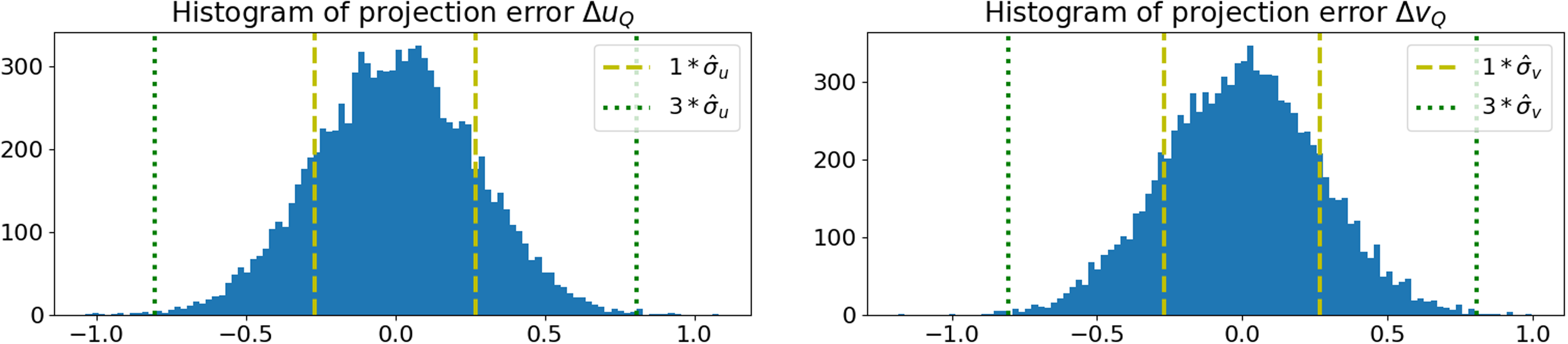
The set of projection errors obtained throughout simulations are displayed in a histogram to confirm if its distribution fits a Gaussian random variable. The standard deviation of the set of projection errors is also computed to compare with the corresponding predicted variance
 $ {Q}_{UV}$
.
Another type of validation pursued in the current work consisted of a simple navigation experiment with a commercial camera. Initially, the intrinsic parameters of the camera were estimated with the function calibrateCameraExtended from the OpenCV library (Bradski, Reference Bradski2000). The estimated intrinsic parameters from the calibration resulted in
 $ {\hat{f}\!}_{u}=1046.0$
px,
 $ {\hat{f}\!}_{v}=1039.0$
px,
 $ {\hat{u}}_{c}=961.9$
px and
 $ {\hat{v}}_{c}=718.4$
px with corresponding standard deviation parameters
 $ {\sigma }_{cam}=[2.66\,{\text px}, 2.53\,{\text px},1.90\,{\text px},2.24\,{\text px}]^{T}$
. After the intrinsic calibration, the camera was installed in the middle of the main window from the vessel’s cabin. Figure 2 shows the main dimensions from the vessel and the installation of the camera.
Vessel dimensions (left) and camera installation (right).

Note that the cabin is situated at a height of 43.15 m, the size of the window is approximately 0.70 m and the draft at the camera position was approximately 10.53 m. The displacement between the GNSS receiver and the camera within the cabin were neglected. Thus, referencing the external frame at the sea level, the camera position was estimated as
 $ {p}_{sc'}^{s}=[0.00{\,}{\text m},0.00{}{\text m},(43.15{\,}{\text m}-0.35{\,}{\text m})-10.53{\,}{\text m}{]}^{T}$
. The camera was supposed to be aligned with the ship frame. However, angular errors were perceived after installation. As there were points from visible containers with known dimensions in the camera scene, it was possible to refine the camera orientation in the ship frame after installation. For each block of containers, estimations for the camera position and orientation with respect to each container frame were computed. The camera orientation with respect to the ship frame was approximated by the mean orientation between all blocks of containers. Figure 3 illustrates this estimation, overlaying the axes of each container frame.
Orientation refinement with point correspondances from containers.

The resulting rotation matrix
 $ {R}_{s}^{c'}$
describing the camera orientation in the ship frame is:
 $$R_s^{c'} = \left[ {\matrix{ { - 0.02153292} \hfill & { - 0.99935245} \hfill & {0.02882714} \hfill \cr { - 0.10928338} \hfill & { - 0.02630829} \hfill & { - 0.99366243} \hfill \cr {0.99377738} \hfill & { - 0.02454678} \hfill & { - 0.10864612} \hfill \cr } } \right].$$
The position and orientation of the vessel in the environment was determined at different points of its trajectory from onboard GNSS measurements. A set of external points were defined from a nautical chart with coordinates described in a Mercator projection. Then, these points are projected into the image recorded by the camera and the corresponding variance
 $ {Q}_{UV}$
is computed from Equation (29). A predicted standard deviation radius
 $ {r}_{\Delta }$
is defined from the square root of its trace:
 $${Q_{UV}} = \left[ {\matrix{ {{q_{{\Delta }00}}} \hfill & {{q_{{\Delta }01}}} \hfill \cr {{q_{{\Delta }10}}} \hfill & {{q_{{\Delta }11}}} \hfill \cr } } \right] \Rightarrow \left[ {\matrix{ {{{\hat \sigma }_{{\Delta }u}}} \hfill \cr {{{\hat \sigma }_{{\Delta }v}}} \hfill \cr } } \right] \approx \left[ {\matrix{ {\sqrt {{q_{{\Delta }00}}} } \hfill \cr {\sqrt {{q_{{\Delta }11}}} } \hfill \cr } } \right],{{\;\;\;\;}}{r_{\Delta }} = \sqrt {\hat \sigma _{{\Delta }u}^2 + \hat \sigma _{{\Delta }v}^2}. $$
The standard deviations of both components are approximated by
 $ {r}_{\Delta }$
, so that each observation in the experiment must be within a circle around the estimated projection. Particularly, circles with radius
 $ 1\cdot {r}_{\Delta }$
,
 $ 2\cdot {r}_{\Delta }$
and
 $ 3\cdot {r}_{\Delta }$
are drawn around each projection to check if each observation is indeed within the predicted interval. Note that it is highly unlikely that the projection error is bigger than three standard deviations. Theoretically, the probability that the observation is within an interval of one, two and three standard deviations from the estimation are 68%, 95% and 99.7%; respectively.
4. Results
4.1. Numerical validation with Gaussian random variables
The camera was described by estimated intrinsic parameters
 $ {\hat{f}\!}_{u}=1000{\,}{p}{x}$
,
 $ {\hat{f}\!}_{v}=1000{\,}{p}{x}$
,
 $ {\hat{u}}_{c}=1100{\,}{p}{x}$
and
 $ {\hat{v}}_{c}=700{\,}{p}{x}$
. The estimated point
 $ Q'$
was defined with coordinates
 $ {p}_{wQ'}^{w}=[5000{\,}{m},250{\,}{m},30{\,}{m}{]}^{T}$
at the external frame
 $ w$
, the estimated ship position was defined with coordinates
 $ {p}_{ws'}^{w}=\left[2000{\,}{m},100{\,}{m},0{\,}{m}\right],$
and the estimated camera position in ship frame
 $ s$
was defined with coordinates
 $ {p}_{sc'}^{s}=[50{\,}{m},0{\,}{m},30{\,}{m}{]}^{T}$
. For simplicity, estimated frames were aligned with each other as described by the following rotation matrices:
 $$R_w^{s'} = \left[ {\matrix{ 1 \hfill & 0 \hfill & 0 \hfill \cr 0 \hfill & 1 \hfill & 0 \hfill \cr 0 \hfill & 0 \hfill & 1 \hfill \cr } } \right]{{\;\;\;\;}},\;\;R_s^{c'} = \left[ {\matrix{ 0 \hfill & { - 1} \hfill & 0 \hfill \cr 0 \hfill & 0 \hfill & { - 1} \hfill \cr 1 \hfill & 0 \hfill & 0 \hfill \cr } } \right].$$
Consider initially a set of error parameters representing a very accurate setup: the camera intrinsic parameters are assumed to be known within one-tenth of a pixel accuracy; the coordinates of the reference point
 $ Q$
are assumed to be known within milimeter accuracy; the ship and camera position are assumed to be known within milimeter accuracy; the ship and camera orientation are assumed to be known within a hundredth of a degree.
 $${\sigma _{fu}} = {\sigma _{fv}} = {\sigma _{uc}} = {\sigma _{vc}} = 0.1{{\;px\;\;\;\;}},\;\;{\sigma _{pqx}} = {\sigma _{pqy}} = {\sigma _{pqz}} = 1{\rm{\;mm}},$$
 $$ {\sigma }_{psx}={\sigma }_{psx}={\sigma }_{psx}={\sigma }_{pcx}={\sigma }_{pcx}={\sigma }_{pcx}=1\,\rm{m}\rm{m},$$
 $$ {\sigma }_{s\phi }={\sigma }_{s\theta }={\sigma }_{s\psi }={\sigma }_{c\phi }={\sigma }_{c\theta }={\sigma }_{c\psi }=0.0{1}^{\circ }.$$
In these conditions, the computation of the predicted variance
 $ {Q}_{UV}$
from Equation (29) resulted in:
 $${Q_{UV}} \approx \left[ {\matrix{ {7.2 \cdot {{10}^{ - 2}}} \hfill & {3.2 \cdot {{10}^{ - 5}}} \hfill \cr {3.2 \cdot {{10}^{ - 5}}} \hfill & {7.2 \cdot {{10}^{ - 2}}} \hfill \cr } } \right] \Rightarrow \left[ {\matrix{ {{{\hat \sigma }_{{\Delta }u}}} \hfill \cr {{{\hat \sigma }_{{\Delta }v}}} \hfill \cr } } \right] \approx \left[ {\matrix{ {0.27} \hfill \cr {0.27} \hfill \cr } } \right].$$
For 10,000 samples, the distribution of projection errors are shown in Figure 4. The standard deviations
 $ {\sigma }_{\Delta u}$
and
 $ {\sigma }_{\Delta v}$
from the set of projection errors in each component are
 $ 0.27$
and
 $ 0.27$
, respectively.
Distribution from projection errors
 $ \Delta {u}_{Q}$
(left) and
 $ \Delta {v}_{Q}$
(right).

The dashed vertical line represents the predicted standard deviation of each component, and the dotted vertical line is three times its magnitude. Recall that for a Gaussian random variable with mean
 $ \mu $
and variance
 $ \sigma $
, the probability that a sample
 $ x$
is inside an interval
 $ [\mu -3\sigma, \mu +3\sigma ]$
is approximately 99.73%. Accordingly, the number of trials which resulted in projection errors
 $ \Delta {u}_{Q}$
,
 $ \Delta {v}_{Q}$
within intervals
 $ [-3{\hat{\sigma }}_{\Delta u},3{\hat{\sigma }}_{\Delta u}]$
and
 $ [-3{\hat{\sigma }}_{\Delta v},3{\hat{\sigma }}_{\Delta v}]$
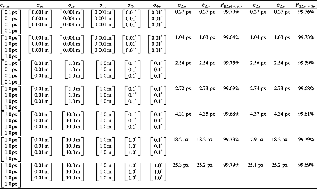
are 9967 and 9976, respectively. These represents 99.67% and 99.76% of the samples. Table 1 presents a summary of different simulations with 10,000 samples each. In each simulation, input standard deviations were modified. The frequency of samples with projection error within the interval of
 $ \pm 3\sigma $
are denoted by
 $ {P}_{\left(\right|\Delta u|\lt 3\sigma )}$
and
 $ {P}_{\left(\right|\Delta v|\lt 3\sigma )}$
.
Comparison between (
 $ {\sigma }_{\Delta u}$
,
 $ {\sigma }_{\Delta v}$
) and (
 $ {\hat{\sigma }}_{\Delta u}$
,
 $ {\hat{\sigma }}_{\Delta v}$
) with different input errors and the same estimated operation condition

In all cases, the predicted standard deviation was close to the actual standard deviation. Further, the frequency of samples within the interval delimited by three standard deviations agrees with the distribution of a Gaussian random variable. Note that all entries were determined around the same operation point. In view of Equation (29), the matrices
 $ {H}_{I}$
,
 $ {H}_{P}$
,
 $ {H}_{pos}$
,
 $ {H}_{ss'}$
and
 $ {H}_{cc'}$
were the same throughout all simulations. To validate the model in different operation points, other simulations were performed with the same set of input error parameters for different estimated ship positions. This implies that matrices
 $ {Q}_{I}$
,
 $ {Q}_{pos}$
,
 $ {Q}_{ss'}$
and
 $ {Q}_{cc'}$
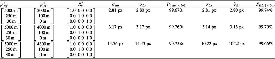
from Equation (29) were fixed, unlike in previous simulations. Table 2 presents a similar simulation summary for the following set of input error parameters:
 $$ {\sigma }_{fu}={\sigma }_{fv}={\sigma }_{uc}={\sigma }_{vc}=1.0\,\rm{p}\rm{x},{\sigma }_{pqx}={\sigma }_{pqy}={\sigma }_{pqz}=1\,\rm{c}\rm{m},$$
 $$ {\sigma }_{psx}={\sigma }_{psx}={\sigma }_{psx}={\sigma }_{pcx}={\sigma }_{pcx}={\sigma }_{pcx}=1\,\rm{m},$$
 $$ {\sigma }_{s\phi }={\sigma }_{s\theta }={\sigma }_{s\psi }={\sigma }_{c\phi }={\sigma }_{c\theta }={\sigma }_{c\psi }=0.{1}^{\circ }.$$
Comparison between (
 $ {\sigma }_{\Delta u}$
,
 $ {\sigma }_{\Delta v}$
) and (
 $ {\hat{\sigma }}_{\Delta u}$
,
 $ {\hat{\sigma }}_{\Delta v}$
) with different operation conditions and the same input errors

Still, in all cases, the predicted standard deviation was close to the actual standard deviation. These indicate that the projection error distribution can be indeed considered an apparently Gaussian random variable with zero mean and variance
 $ {Q}_{UV}$
in these ranges of parameters. It is also interesting to note that the projection error increases when the point
 $ Q'$
is closer to the camera because the elements from matrices
 $ {H}_{I}$
and
 $ {H}_{P}$
are proportional to
 $ ({p}_{cQ'}^{cz}{)}^{-1}$
.
4.2. Validation with navigation experiment
The validation with the navigation experiment was performed with images from the video recorded by the camera. Considering the dimensions of the ship cabin, the maximum position error in the camera were defined as
 $ \pm $
3 m. The maximum angular error in the camera were defined as
 $ \pm {1}^{\circ }$
given the proposed refinement with the containers blocks, which assumes that they are aligned with the ship frame. Therefore, assuming that such errors are within the aforementioned bounds with an approximate
 $ 99.73{\%}$
probability:
 $${\sigma _{pc}} = {\left[ {\matrix{ {{3 \over 3}{\rm{m}}\;{3 \over 3}{\rm{m}}\;{3 \over 3}{\rm{m}}} } } \right]^{T}}, {\sigma _{\Phi c}} = {\left[ {\matrix{ {{{{1 \over 3}}^{^\circ} }\;{{{1 \over 3}}^{^\circ} }\;{{{1 \over 3}}^{^\circ} }} \hfill \cr } } \right]^{T}}.$$
The ship position and orientation at the time of each image was determined by an onboard GNSS equipment. Figure 5 shows the input image side by side with the GNSS instantaneous measurement.
Input image overlaid with corresponding GNSS measurement.

Assuming that the ship roll and pitch angles are zero, the position of the ship and its orientation
 $ {R}_{w}^{s'}$
in mercator coordinates are described by:
 $$p_{ws'}^w = \left[ {\matrix{ { - 4869712.77\,{\rm{m}}} \hfill \cr { - 2634539.79\,{\rm{m}}} \hfill \cr {\;\;\;\;\;\;0.00\,{\rm{m}}} \hfill \cr } } \right]{\,},\;\;R_w^{s'} = \left[ {\matrix{ {0.99718513} \hfill & {0.07497873} \hfill & {0.0} \hfill \cr { - 0.07497873} \hfill & {0.99718513} \hfill & {0.0} \hfill \cr {\;\;\;\;\;\;\;\;0.0} \hfill & {\;\;\;\;\;\;0.0} \hfill & {1.0} \hfill \cr } } \right].$$
From the heading resolution, the maximum error in the yaw angle of the vessel was considered to be
 $ \pm \!0.{1}^{\circ }$
. Regarding roll and pitch angles, we assumed that these angular errors did not exceed
 $ \pm {\!\!1}^{\circ }$
. For a typical GNSS setup that can provide an accuracy better than 10 m around harbour areas (Zalewski et al., Reference Zalewski, Bąk and Bergmann2022) and assuming a small time desynchronisation considering the vessel’s speed, we defined a maximum horizontal position error of
 $ \pm\! 20\,$
m for the vessel. The maximum vertical position error was defined as
 $ \pm\! $
3 m given potential unknown variations in the regional tide. Again, for a 99.7% probability that errors are within the proposed bounds:
 $${\sigma _{ps}} = {\left[ {\matrix{ {{{20} \over 3}\,{\rm{m}}} \hfill & {{{20} \over 3}\,{\rm{m}}} \hfill & {{3 \over 3}\,{\rm{m}}} \hfill \cr } } \right]^T}{\,},\;\;{\sigma _{\Phi s}} = {\left[ {\matrix{ {{{{1 \over 3}}^{^\circ }}} \hfill & {{{{1 \over 3}}^{^\circ }}} \hfill & {{{{{0.1} \over 3}}^ {^\circ }}} \hfill \cr } } \right]^T}.$$
Regarding the reference points to be projected at the scene, note that at the left part from the image there is a visible island and at the right part from the image there is another region with land. Four points from this island (Q1 to Q4) and a point from the right region (Q5) were selected as references to be projected. Figure 6 illustrates the representation of these points in the nautical chart around the Paranagua Port (state of Parana, Brazil), where the experiment were recorded.
Nautical chart representation of the experiment region (left) and location of points
 $ Q1-Q5$
(right).

Mercator coordinates for each point at the nautical chart are given by:
 $$\matrix{ & {p_{wQ1'}^w = \left[ {\matrix{ { - 4867311.97\,{\rm{m}}} \hfill \cr { - 2632890.34\,{\rm{m}}} \hfill \cr \,\,\,\,\,\,{\;\;\;0.00\,{\rm{m}}} \hfill \cr } } \right]{\,},\;\;p_{wQ2'}^w = \left[ {\matrix{ { - 4867109.74\,{\rm{m}}} \hfill \cr { - 2633105.22\,{\rm{m}}} \hfill \cr \,\,\,\,\,\,{\;\;\;55.00\,{\rm{m}}} \hfill \cr } } \right]} \hfill \cr& {p_{wQ3'}^w = \left[ {\matrix{ { - 4867173.92\,{\rm{m}}} \hfill \cr { - 2633698.93\,{\rm{m}}} \hfill \cr \,\,\,\,{\;\;\;51.00\,{\rm{m}}} \hfill \cr } } \right]{\,},\;\;p_{wQ4'}^w = \left[ {\matrix{ { - 4867114.83\,{\rm{m}}} \hfill \cr { - 2633871.45\,{\rm{m}}} \hfill \cr \,\,\,\,{\;\;\;0.00\,{\rm{m}}} \hfill \cr } } \right]} \hfill \cr& \quad\quad\quad\quad\quad\quad\quad\quad\quad\quad\quad\quad\;\;\;{p_{wQ5'}^w = \left[ {\matrix{ { - 4865664.29\,{\rm{m}}} \hfill \cr { - 2637003.29\,{\rm{m}}} \hfill \cr \,\,\,\,{\;\;\;0.00\,{\rm{m}}} \hfill \cr } } \right].} \hfill \cr } $$
Position errors in the Mercator coordinates of each point were neglected in this experiment:
 $${\sigma _{pq}} = {\left[ {\matrix{ {{0 \over 3}\,{\rm{m}}\;{0 \over 3}\,{\rm{m}}\;{0 \over 3}\,{\rm{m}}} \hfill \cr } } \right]^T}.$$
Figure 7 presents the projections of points Q1 to Q5 using Equations (2) and (14). Each point is projected around circles with radius
 $ 1\cdot {r}_{\Delta }$
,
 $ 2\cdot {r}_{\Delta }$
and
 $ 3\cdot {r}_{\Delta }$
in colors blue, yellow and green, respectively. The standard deviation radius
 $ {r}_{\Delta }$
was computed from Equations (29) and (33).
Projection of points
 $ Q1-Q5$
encompassed by respective confidence bounds.

Note that points
 $ Q1$
to
 $ Q4$
are contained in the 95% confidence interval defined by the circle with radius
 $ 2\cdot {r}_{\Delta }$
, and
 $ Q5$
are within the 68% confidence interval defined by the circle with radius
 $ 1\cdot {r}_{\Delta }$
. Therefore, as expected, all observations are within the confidence bounds given by the predicted variance
 $ {Q}_{UV}$
.
5. Discussion
The simulation experiments were conducted at various operating points that satisfy the assumptions made during the development of Equation (29). Regarding the angular parameters, the proposed projection error model is recommended for use with angular errors smaller than 10 degrees. The primary assumption is that the angular errors are sufficiently small such that the rotation matrix describing the transformation between the estimated and real frames can be approximated by Equations (15) and (16) (i.e. neglecting quadratic angular error terms).
Concerning the remaining error parameters of the tracking system, it is assumed that the errors in each parameter are significantly smaller than the corresponding estimated parameter. Generally, it is recommended that each error should be at most one-tenth of its corresponding parameter. These assumptions are reasonable when the virtual points projected onto the scene are far from the camera. However, for the projection of virtual points near the camera, this assumption may become problematic and requires further detailed verification. Notably, in the third row of Table 2, a larger discrepancy can be observed between the predicted variance
 $ {\hat{\sigma }}_{\Delta u}$
(
 $ \approx 14.45$
px) and the obtained standard-deviation
 $ {\sigma }_{\Delta u}$
(
 $ \approx 14.36$
px) compared to the other rows in the same table.
With respect to the real experiment conducted, we demonstrated that each reference point was observed near its corresponding estimated projection within the proposed predicted radius bound
 $ {r}_{\Delta }$
(Equation (33)). This result suggests that the proposed projection error model is suitable for real-world applications. However, it is important to note that, the camera is assumed to be fixed in the ship frame without a need for tracking it in real-time. Therefore, it is crucial to ensure that the camera remains static relative to the ship during operation through proper installation. If the camera’s position and orientation within the ship frame are estimated in real time by a tracking component, the impact of variations can be significantly mitigated. Furthermore, a rigid-body model for the ship is implicitly assumed. Additionally, the possibility of camera vibration has not been considered here.
The following sections briefly describe potential applications of the proposed projection error model, which are suggested for further investigation in future work.
5.1. Real-time error projection
To use AR projections to assist in navigation tasks, operators need at least a sense of how reliable the projection of each virtual element is. For example, in cases with low visibility of the scene, following a virtual projection without such accuracy assessment may lead to actual route deviations. Thus, a straightforward application for the proposed projection model is the real-time visualisation of error estimations with translucent circles, as shown in Figure 7. It does not require any mental computation or significant interpretation to perceive where a point of interest might be in the scene. Note that the use of an AR system by itself helps in the identification of points of interest at the navigation scene with less cognitive load. Complementary, the proposed error representation enables the readily identification of the corresponding accuracy for each virtual element projection.
Moreover, the use of the proposed error representation in real time may assist in the detection of failures in other onboard navigation equipment. For example, if a navigation equipment loses performance when outputting higher standard deviation errors to the AR system, the corresponding circles of projection error will immediately become bigger and be easily perceived. On the other hand, if a piece of equipment loses performance and does not increase its standard deviation error, the observation of a point of interest at the scene will be seen outside the corresponding projection error circle. Such discrepancy may be detected in cases with high visibility of the scene.
5.2. Prediction of AR system performance
There are many potential definitions that may be formulated to characterise an AR system performance. For navigational assistance, the correct positioning of virtual elements seems the most important feature as it is critical to ensure that the vessel follows its planned trajectory. Therefore, the magnitude of the projection error is proposed as the principal performance parameter to characterise AR system setups in this technical context.
A simple simulation is proposed to exemplify a method of predicting the overall projection errors for different AR error setups. The vessel was assumed to be in a fixed position
 $ {p}_{ws'}^{w}=[2000\,\rm{m},0\,\rm{m},0\,\rm{m}{]}^{T}$
with a camera installed at the vessel with estimated position
 $ {p}_{sc'}^{s}=[50\,\rm{m},0\,\rm{m},30\,\rm{m}{]}^{T}$
and described by estimated intrinsic parameters
 $ {\hat{f}\!}_{u}=1000\,\rm{p}\rm{x}$
,
 $ {\hat{f}\!}_{v}=1000\,\rm{p}\rm{x}$
,
 $ {\hat{u}}_{c}=1100\,\rm{p}\rm{x}$
,
 $ {\hat{v}}_{c}=700\,\rm{p}\rm{x}$
. Several points
 $ Q'$
were defined from a region of interest, and the predicted standard deviation
 $ {\hat{\sigma }}_{\Delta u}$
and
 $ {\hat{\sigma }}_{\Delta v}$
were computed for each point
 $ Q'$
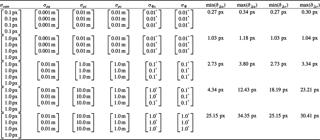
. As the projection error is bounded by three predicted standard deviations with a 99.7% probability, the maximum projection error in the whole region may be estimated as 3 times the maximum predicted standard deviations throughout the simulation. Table 3 presents the minimum and maximum predicted standard deviations for different input error parameters in a region parametrised by the following minimum and maximum values in each axis:
 $ [{x}_{min},{x}_{max}]=[{3,000}\,\rm{m},{5,000}\,\rm{m}]$
,
 $ [{y}_{min},{y}_{max}]=[-500\,\rm{m},500\,\rm{m}]$
and
 $ [{z}_{min},{z}_{max}]=[0\,\rm{m},0\,\rm{m}]$
.
Minimum and maximum predicted (
 $ {\hat{\sigma }}_{\Delta u}$
,
 $ {\hat{\sigma }}_{\Delta v}$
) computed from region of interest with different input errors

Clearly, the first row represents a better setup than the last row of Table 3. In the case represented by the first row of Table 3, the projection error in the whole region should be less than 1 px; while in the case represented by the last row of Table 3, the projection error in the whole region should be less than 100 px. Note that the magnitude of errors
 $ {\sigma }_{cam}$
depends on the camera technology and the calibration method while the rest of the errors depends on the tracking and integration technologies used by the AR system. Therefore, from performance parameters of the tracking system it is possible to quantitatively predict the expected projection error of the AR system.
5.3. Specification of AR accuracy requirements
Consider again Table 3 from the previous section. In addition to predicting the expected error of different potential AR systems setups, note that it is possible to specify requirements that ensures a desired projection error. If the AR system needs to perform with a projection error inferior than 1 px, then a possible set of accuracy requirements for each parameter may be defined by the input errors from the first row of Table 3:
 $$\matrix{ {\sigma _{cam}^{1px} \le \left[ {\matrix{ {0.1{\rm{\;px}}} \hfill \cr {0.1{\rm{\;px}}} \hfill \cr {0.1{\rm{\;px}}} \hfill \cr {0.1{\rm{\;px}}} \hfill \cr } } \right]\;\;,\;\;\sigma _{pq}^{1px} \le \left[ {\matrix{ {0.001{\rm{\;m}}} \hfill \cr {0.001{\rm{\;m}}} \hfill \cr {0.001{\rm{\;m}}} \hfill \cr } } \right]\;\;,\;\;\sigma _{ps}^{1px} \le \left[ {\matrix{ {0.01{\rm{\;m}}} \hfill \cr {0.01{\rm{\;m}}} \hfill \cr {0.01{\rm{\;m}}} \hfill \cr } } \right]\;\;,\;\;\sigma _{pc}^{1px} \le \left[ {\matrix{ {0.01{\rm{\;m}}} \hfill \cr {0.01{\rm{\;m}}} \hfill \cr {0.01{\rm{\;m}}} \hfill \cr } } \right]} \hfill \cr \quad\quad\quad\quad\quad\quad\quad\quad\quad\quad\quad\quad\quad\quad\quad\quad\quad\quad\quad{\sigma _{\Phi s}^{1px} \le \left[ {\matrix{ {{{0.01}^ \circ }} \hfill \cr {{{0.01}^ \circ }} \hfill \cr {{{0.01}^ \circ }} \hfill \cr } } \right]\;\;,\quad\sigma _{\Phi c}^{1px} \le \left[ {\matrix{ {{{0.01}^ \circ }} \hfill \cr {{{0.01}^ \circ }} \hfill \cr {{{0.01}^ \circ }} \hfill \cr } } \right].} \hfill \cr } $$
Alternatively, if a maximum projection error of 10 px is acceptable, the respective requirements of accuracy are given by the input errors from the third row of Table 3:
 $$\matrix{ {\sigma _{cam}^{10px} \le \left[ {\matrix{ {1.0{\rm{\;px}}} \hfill \cr {1.0{\rm{\;px}}} \hfill \cr {1.0{\rm{\;px}}} \hfill \cr {1.0{\rm{\;px}}} \hfill \cr } } \right]\;\;,\;\;\sigma _{pq}^{10px} \le \left[ {\matrix{ {0.01{\rm{\;m}}} \hfill \cr {0.01{\rm{\;m}}} \hfill \cr {0.01{\rm{\;m}}} \hfill \cr } } \right]\;\;,\;\;\sigma _{ps}^{10px} \le \left[ {\matrix{ {1.0{\rm{\;m}}} \hfill \cr {1.0{\rm{\;m}}} \hfill \cr {1.0{\rm{\;m}}} \hfill \cr } } \right]\;\;,\;\;\sigma _{pc}^{10px} \le \left[ {\matrix{ {1.0{\rm{\;m}}} \hfill \cr {1.0{\rm{\;m}}} \hfill \cr {1.0{\rm{\;m}}} \hfill \cr } } \right]} \hfill \cr\quad\quad\quad\quad\quad\quad\quad\quad\quad\quad\quad\quad\quad\quad\quad\quad\quad\quad\quad {\sigma _{\Phi s}^{10px} \le \left[ {\matrix{ {{{0.1}^ \circ }} \hfill \cr {{{0.1}^ \circ }} \hfill \cr {{{0.1}^ \circ }} \hfill \cr } } \right]\;\;,\quad\sigma _{\Phi c}^{10px} \le \left[ {\matrix{ {{{0.1}^ \circ }} \hfill \cr {{{0.1}^ \circ }} \hfill \cr {{{0.1}^ \circ }} \hfill \cr } } \right].} \hfill \cr } $$
The definition of how much projection error is acceptable for a navigational assistance application is beyond the scope of the current work. Note that Table 3 data were computed with just a few AR setups to concisely exemplify this procedure. Ideally, more conditions should be considered with different input errors accordingly to typical uncertainties of consolidated tracking technologies.
6. Conclusion
A simple projection error model was derived from the subtraction of two pinhole camera models. One set of parameters was assumed to be the real parameters while the another was the corresponding estimations. Simplifications were proposed to reach a simple matricial equation. Errors in the parameters from the pinhole camera model were assumed to be Gaussian random variables with zero mean and non-zero covariances, which resulted in a projection error distributed by a Gaussian random variable with zero mean and non-zero covariance as well. The proposed projection error model was validated with numerical simulations and a real navigation experiment near the Paranagua Port in the state of Parana, Brazil.
Potential applications for the proposed projection error model were discussed. It can be used as a complement to a virtual element projection by informing its accuracy in real time. Additionally, it may be used as a means to detect sensor failures throughout navigation considering a full integration with other equipment from a vessel. These may assist in the overall reliability and safety of maritime navigation. Furthermore, the proposed model may assist the characterisation and design of maritime navigational assistance AR systems. A simple simulation was implemented to exemplify the procedure of predicting maximum projection errors that may arise in the projection of virtual elements. This could be used to assess the suitability of potential components within the implementation of an AR system.
Generally, the authors suggests that AR researchers within maritime domains should focus on the development of design methodologies that ensures the reliability required by this industry. In contrast to other AR applications, it is not possible to modify the environment arbitrarily with markers. Further, typical distances of visible features and projected elements are significantly greater. For maritime navigational assistance, the correct positioning of virtual elements into the scene is critical. Movements are typically subject to wave-induced oscillations. Such factors poses significant challenges for the reliable operation of AR systems in maritime scenarios.
Acknowledgements
The authors thank Petrobras and Brazilian National Agency for Petroleum, Natural Gas and Biofuels (ANP) for supporting this research project (process 2018/00402-5). B.G.L. thanks the Coordination for the Improvement of Higher Education Personnel (CAPES) for the scholarship during the first year of the project. E.A.T. thanks the CNPq – Brazilian National Council for Scientific and Technological Development for the research grant (process 310127/2020-3).
Competing interests
All authors declare that there are no other competing interests.