


1 Introduction
In many animals, locomotion emerges from the interplay of the active material properties of an organisms’ musculature and the passive material properties of their flexible body or appendage. Elastic structures that bend and flex can be thought of as mechanical systems with their own natural frequency of vibration, or the frequency at which the a system oscillates in free vibration. Since maximum deformations are generated when a flexible structure is driven at its natural frequency, it has been suggested that locomotory efficiency and performance is also maximized at this frequency (Alexander & Bennet-Clark Reference Alexander and Bennet-Clark1977). The basis for this argument is that when an animal’s muscular processes are tuned to the elastic properties of their locomotory structures, the potential energy stored in the elastic structures during muscular deformation is maximized. The cessation of muscular activity in turn releases the stored potential energy and further drives the motion of the structure.
For swimming and flying animals, fluid motion also plays a significant role in determining the efficiency of locomotion. Independent and sometimes counter to the argument that performance is maximized when a structure is driven at its natural frequency, it is conjectured that locomotory performance is enhanced when the movement of the structure is tuned to nonlinear fluid effects, such as drag reduction (Ramananarivo, Godoy-Diana & Thiria Reference Ramananarivo, Godoy-Diana and Thiria2011) or pressure-induced suction (Gemmell et al. Reference Gemmell, Colin, Costello and Dabiri2015a ). On the other hand, resonant driving can enhance the transfer of momentum from the structure to the local fluid environment and lead to the formation strong vortex structures to drive the organism forward (Hoover et al. Reference Hoover, Cortez, Tytell and Fauci2018). Other arguments suggest that while resonance may play a large role with certain body shapes, other body shapes do not benefit due to effects of fluid damping (Tytell et al. Reference Tytell, Hsu, Williams, Cohen and Fauci2010). The debate behind these two camps suggests the need for high fidelity models that incorporate both the nonlinear effects from the surrounding fluid environment and the elastic structures that account for the morphology and mechanical properties of the organism.
Jellyfish locomotion can be a characterized as a process of active elastic deformation of a bell and passive recoil (Hoover & Miller Reference Hoover and Miller2015). The propulsive cycle of forward swimming jellyfish is initiated by the contraction of the coronal swimming muscles present in the subumbrellar cavity of the bell. This muscular contraction deforms the bell and pushes fluid out of the bell cavity, forming a starting vortex ring in the wake of the jellyfish. Following the cessation of muscular activity, the bell’s passive elastic properties, which are due to the mechanical properties of the mesoglea (Arai Reference Arai1997), drive the expansion of the bell to its resting state. The expansion of the bell refills it with fluid. During this passive expansion, the motion of the bell margin forms a stopping vortex ring, which is rotating in the opposite direction of the starting vortex ring (Gemmell, Costello & Colin Reference Gemmell, Costello and Colin2014). The interaction between the starting and stopping vortex rings directs fluid from a region outside of the bell’s immediate wake upward into the bell cavity (Hoover, Griffith & Miller Reference Hoover, Griffith and Miller2017). This process, known as passive energy recapture (Gemmell et al. Reference Gemmell, Costello, Colin, Stewart, Dabiri, Tafti and Priya2013), allows for a secondary source of thrust at no additional metabolic cost for the jellyfish. This vortex ring dynamics is particularly important for oblate jellyfish with a low fineness ratio where the stopping vortex ring continues to drive the bell forward and direct prey towards feeding structures. It has been suggested that this dynamic has allowed jellyfish to reach sizes that surpass the phylogenetic constraints of their musculature (Dabiri et al. Reference Dabiri, Colin, Costello and Gharib2005a ,Reference Dabiri, Gharib, Colin and Costello b ; Dabiri, Colin & Costello Reference Dabiri, Colin and Costello2007).
A number of studies have considered jellyfish locomotion in the context of resonant driving. Demont & Gosline (Reference Demont and Gosline1988) first noted the phenomena and used a reduced-order lumped parameter model to characterize the bell as a spring–mass–damper system, with linear damping terms to describe the viscoelastic mesoglea and the shear of the surrounding fluid. Applying a sinusoidal force at the resonant frequency resulted in a 40 % increase in the amplitude of the circumferential oscillation when compared to frequencies significantly above and below. Megill, Gosline & Blake (Reference Megill, Gosline and Blake2005) further added to the model by incorporating nonlinear spring elements that account for large strains. Recently, Hoover & Miller (Reference Hoover and Miller2015) approached this problem numerically by solving the fully coupled fluid–structure interaction problem. Using a two-dimensional (2-D) elastic bell immersed in a viscous fluid, they found that driving near the resonant frequency produced a 50 % increase in swimming speed relative to below the resonant frequency driving and even more gains when compared to frequencies significantly above the resonant frequency. There were several limitations of this model. The bell was driven using a sinusoidal driving force that actively re-expanded it, and the 2-D model was only applied to the study of prolate bells, as the fluid dynamics of oblate bells is not well characterized in two dimensions (Herschlag & Miller Reference Herschlag and Miller2011).
A number of other computational studies have examined the fluid dynamics behind jellyfish swimming (Zhao, Freund & Moser Reference Zhao, Freund and Moser2008; Huang & Sung Reference Huang and Sung2009). Sahin & Mohseni (Reference Sahin and Mohseni2009) modelled the bell using an axisymmetric Lagrangian–Eulerian formulation to simulate the forward swimming of Aequorea victoria using recorded bell profiles. Herschlag & Miller (Reference Herschlag and Miller2011) tested Reynolds number effects using 2-D immersed boundary jellyfish models of oblate and prolate bells. Park et al. (Reference Park, Chang, Huang and Sung2014) used a penalty immersed boundary method to drive the bell motion and explore wake structures. Alben, Miller & Peng (Reference Alben, Miller and Peng2013) used a combination of computational tools and analytical models to quantify the kinematics of the bell for both high swimming and high efficiency movements. These studies did not specifically quantify the interplay between the bell’s material properties and passive energy recapture since the kinematics were prescribed or simplified.
Recently, Hoover et al. (Reference Hoover, Griffith and Miller2017) developed a computational three-dimensional (3-D) immersed boundary model of a forward swimming jellyfish whose kinematics are a consequence of the interaction between the bell’s material properties and the local fluid dynamics. In that study, the bell’s passive elastic and active muscular material properties were varied, and their effects on swimming performance were quantified. It was noted that the relative strength of the muscular contraction determined the strength and speed of advection of the vortex rings. However, this study did not examine the effects of passive energy recapture by varying the driving period.
In this study, we quantify the relationship between the driving frequency, the dynamics of passive energy recapture and the resulting locomotory efficiency of jellyfish using the 3-D numerical model described in Hoover et al. (Reference Hoover, Griffith and Miller2017). First, we extract the period of free vibration for bells of differing material properties. We then drive the bell over a range of frequencies using a strength of muscular activation that is proportional to the effective stiffness of the bell. The frequencies are varied by fixing the duration of active contraction and varying the length of time the muscles are relaxed. The role of passive energy recapture is then quantified by measuring the strength of the stopping vortex ring. The performance of the bell at a given driving frequency is then quantified by examining the resulting swimming speed and input power. We then use swimming efficiency metrics, such as swimming economy and cost of transport, to compare the performance of bells with varying material properties. An additional study is performed to examine the performance of driving the bell significantly above its natural frequency.
2 Materials and methods
2.1 Fluid–structure interaction
Fluid–structure interaction problems are common to biological systems and have been examined with a variety of computational frameworks. The immersed boundary (IB) method (Peskin Reference Peskin2002; Mittal & Iaccarino Reference Mittal and Iaccarino2005) is an approach to numerically solving fully coupled fluid–structure interaction problems introduced by Peskin to study blood flow in the heart (Peskin Reference Peskin1977). Since then, the IB method has been applied to a variety of fluid–structure interaction problems in biology in the low to intermediate Reynolds number regime, including undulatory swimming (Fauci & Peskin Reference Fauci and Peskin1988; Bhalla et al. Reference Bhalla, Bale, Griffith and Patankar2013; Hoover et al. Reference Hoover, Cortez, Tytell and Fauci2018), insect flight (Miller & Peskin Reference Miller and Peskin2004, Reference Miller and Peskin2005, Reference Miller and Peskin2009; Jones et al. Reference Jones, Laurenza, Hedrick, Griffith and Miller2015), lamprey swimming (Tytell et al. Reference Tytell, Hsu, Williams, Cohen and Fauci2010, Reference Tytell, Leftwich, Hsu, Griffith, Cohen, Smits, Hamlet and Fauci2016), crustacean swimming (Zhang et al. Reference Zhang, Guy, Mulloney, Zhang and Lewis2014) and jellyfish swimming (Hamlet, Santhanakrishnan & Miller Reference Hamlet, Santhanakrishnan and Miller2011; Herschlag & Miller Reference Herschlag and Miller2011; Hoover & Miller Reference Hoover and Miller2015; Hoover et al. Reference Hoover, Griffith and Miller2017).
The IB formulation of fluid–structure interaction uses an Eulerian description of the equations of fluid motion, and it uses a Lagrangian description of the elastic immersed boundaries. Let
 $\boldsymbol{x}=(x,y,z)\in \unicode[STIX]{x1D6FA}$
denote physical Cartesian coordinates, with
 $\unicode[STIX]{x1D6FA}$
denoting the physical region occupied by the fluid–structure system. Let
 $\boldsymbol{X}=(X,Y,Z)\in U$
denote Lagrangian material coordinates that describe the immersed structure, with
 $U$
denoting the Lagrangian coordinate domain. The physical position of material point
 $\boldsymbol{X}$
at time
 $t$
is
 $\unicode[STIX]{x1D74C}(\boldsymbol{X},t)\in \unicode[STIX]{x1D6FA}$
, so that the physical region occupied by the structure at time
 $t$
is
 $\unicode[STIX]{x1D74C}(U,t)\subset \unicode[STIX]{x1D6FA}$
.
The immersed boundary formulation of the equations of motion is given by
 $$\begin{eqnarray}\displaystyle & \displaystyle \unicode[STIX]{x1D70C}\left(\frac{\unicode[STIX]{x2202}\boldsymbol{u}(\boldsymbol{x},t)}{\unicode[STIX]{x2202}t}+\boldsymbol{u}(\boldsymbol{x},t)\boldsymbol{\cdot }\unicode[STIX]{x1D735}\boldsymbol{u}(\boldsymbol{x},t)\right)=-\unicode[STIX]{x1D735}p(\boldsymbol{x},t)+\unicode[STIX]{x1D707}\unicode[STIX]{x1D6FB}^{2}\boldsymbol{u}(\boldsymbol{x},t)+\boldsymbol{f}(\boldsymbol{x},t), & \displaystyle\end{eqnarray}$$
 $$\begin{eqnarray}\displaystyle & \displaystyle \unicode[STIX]{x1D735}\boldsymbol{\cdot }\boldsymbol{u}(\boldsymbol{x},t)=0, & \displaystyle\end{eqnarray}$$
 $$\begin{eqnarray}\displaystyle & \displaystyle \boldsymbol{f}(\boldsymbol{x},t)=\int _{U}\boldsymbol{F}(\boldsymbol{X},t)\,\unicode[STIX]{x1D6FF}(\boldsymbol{x}-\unicode[STIX]{x1D74C}(\boldsymbol{X},t))\,\text{d}\boldsymbol{X}, & \displaystyle\end{eqnarray}$$
 $$\begin{eqnarray}\displaystyle & \displaystyle \int _{U}\boldsymbol{F}(\boldsymbol{X},t)\boldsymbol{\cdot }\boldsymbol{V}(\boldsymbol{X})\,\text{d}\boldsymbol{X}=-\int _{U}\mathbb{P}(\boldsymbol{X},t)\boldsymbol{ : }\unicode[STIX]{x1D735}_{\boldsymbol{X}}\boldsymbol{V}(\boldsymbol{X})\,\text{d}\boldsymbol{X}, & \displaystyle\end{eqnarray}$$
 $$\begin{eqnarray}\displaystyle & \displaystyle \frac{\unicode[STIX]{x2202}\unicode[STIX]{x1D74C}(\boldsymbol{X},t)}{\unicode[STIX]{x2202}t}=\int _{\unicode[STIX]{x1D6FA}}\boldsymbol{u}(\boldsymbol{x},t)\,\unicode[STIX]{x1D6FF}(\boldsymbol{x}-\unicode[STIX]{x1D74C}(\boldsymbol{X},t))\,\text{d}\boldsymbol{x} & \displaystyle\end{eqnarray}$$
in which
 $\unicode[STIX]{x1D70C}$
is the fluid density,
 $\unicode[STIX]{x1D707}$
is the dynamic viscosity,
 $\boldsymbol{u}(\boldsymbol{x},t)=(u_{x},u_{y},u_{z})$
is the Eulerian material velocity field and
 $p(\boldsymbol{x},t)$
is the Eulerian pressure field. Here,
 $\boldsymbol{f}(\boldsymbol{x},t)$
and
 $\boldsymbol{F}(\boldsymbol{X},t)$
are equivalent Eulerian and Lagrangian force densities.
 $\boldsymbol{F}$
is defined in terms of the first Piola–Kirchhoff solid stress in (2.4) using a weak formulation, in which
 $\boldsymbol{V}(\boldsymbol{X})$
is an arbitrary Lagrangian test function. The Dirac delta function
 $\unicode[STIX]{x1D6FF}(\boldsymbol{x})$
appears as the kernel of the integral transforms, equations (2.3) and (2.5), that connect the Eulerian and Lagrangian frames.
In this study, a hybrid finite difference/finite element version of the immersed boundary method (IB/FE) is used to approximate (2.1)–(2.5). The IB/FE method uses a finite difference formulation for the Eulerian equations and a finite element formulation to describe the solid body. More details on the IB/FE method can be found in Griffith & Luo (Reference Griffith and Luo2017).
2.2 Bell model and geometry
In the following subsection, we describe the structural model of the bell. In this study, the bell’s motion is a result of the interaction between the passive elastic material properties of the bell, the active tension generated by the model of the coronal swimming musculature and the interaction with the surrounding fluid. The structural stresses resulting from the bell’s passive and active material properties are calculated using the first Piola–Kirchhoff stress tensor
 $$\begin{eqnarray}\mathbb{P}=\mathbb{P}_{p}+\mathbb{P}_{a}\end{eqnarray}$$
in which
 $\mathbb{P}_{p}$
describes the passive elasticity of the body and
 $\mathbb{P}_{a}$
describes the active tension generated by the muscle.
The passive elastic properties of the bell’s mesoglea are described using a neo-Hookean material model
 $$\begin{eqnarray}\mathbb{P}_{p}=\unicode[STIX]{x1D702}(\mathbb{F}-\mathbb{F}^{-T})\end{eqnarray}$$
in which
 $\mathbb{F}=\unicode[STIX]{x2202}\unicode[STIX]{x1D74C}/\unicode[STIX]{x2202}\boldsymbol{X}$
is the deformation gradient and
 $\unicode[STIX]{x1D702}$
is the elastic modulus of the material.
The contraction and release of the subumbrellar swimming muscles is modelled with time-dependent active stress on the bell. This circumferentially oriented stress is applied over the lower portion of the bell, which is where the coronal swimming musculature is present. The active stress is calculated via
 $$\begin{eqnarray}\mathbb{P}_{a}=JT\mathbb{F}\boldsymbol{f}_{\mathbf{0}}\,\boldsymbol{f}_{\mathbf{0}}^{\text{T}}\end{eqnarray}$$
in which
 $J=\text{det}(\mathbb{F})$
is the Jacobian of
 $\mathbb{F}$
,
 $T$
is the magnitude of the prescribed tension and
 $\boldsymbol{f}_{\mathbf{0}}$
is the (fibre) direction vector of the prescribed tension with respect to the reference configuration. Here
 $\boldsymbol{f}_{\mathbf{0}}$
is chosen to model the coronal orientation of the subumbrellar swimming musculature in the undeformed configuration.
The three-dimensional bell model developed for this study accounts for variations in the bell’s thickness and material properties. Previous models (Daniel Reference Daniel1983; McHenry & Jed Reference McHenry and Jed2003; Sahin, Mohseni & Colin Reference Sahin, Mohseni and Colin2009; Herschlag & Miller Reference Herschlag and Miller2011) have described the bell geometry as a hemiellipsoid or by using functions fit to digitized bell shapes. In this study, the immersed body model is a hemi-ellipsoid bell with both exumbrellar and subumbrellar surfaces. The bell shape was parametrized using a hemiellipsoid description for the exumbrellar (
 $\text{ex}$
) and subumbrellar (
 $\text{sub}$
) surfaces via
 $$\begin{eqnarray}\frac{(X-X_{c})^{2}+(Y-Y_{c})^{2}}{a_{ex,sub}^{2}}+\frac{(Z-Z_{c})^{2}}{b_{ex,sub}^{2}}=1\quad \text{for }Z\geqslant 0,\end{eqnarray}$$
in which
 $\mathbf{X}_{c}=(X_{c},Y_{c},Z_{c})$
is the centre of the ellipsoid,
 $a_{ex,sub}$
is the radial axis of the subumbrellar and exumbrellar surfaces of the bell, respectively, and
 $b_{ex,sub}$
is its vertical axis (see table 1 and figure 1
a). Variation in the bell thickness due to difference in the exumbrellar and subumbrellar dimensions accounts for variation in the elastic profile of the bell, where the thinner bell margin is more flexible than the thicker top of the bell. In all of the numerical studies reported here, as
 $\unicode[STIX]{x1D702}$
is varied,
 $T_{max}$
is also varied by the same proportion. This ensures the same amount of static deformation of the bell.
(a) A diagram of the bell model geometry with major and minor axes for the subumbrellar hemiellipsoid,
 $a_{sub}$
and
 $b_{sub}$
respectively, and the exumbrellar hemiellipsoid,
 $a_{ex}$
and
 $b_{ex}$
. (b) The model geometry draws inspiration from the oblate jellyfish, Aurelia spp. (c) A plot of the spatial parametrization of the musculature,
 $\unicode[STIX]{x1D6FD}$
, relative to the bell height,
 $Z/L_{vert}$
.

Table of dimensional parameters for the bell’s structural model. In this study the elastic modulus,
 $\unicode[STIX]{x1D702}$
, and the maximum tension,
 $T_{max}$
, are varied in proportion to one another and the values reported here are for the reference configuration.

Below we describe how the active muscular tension is applied to the bell. The tension,
 $T$
, applied at point
 $\mathbf{X}$
varies in time and with respect to the height of the bell in its reference configuration,
 $Z$
, and is given by
 $$\begin{eqnarray}T=T_{max}\cdot \unicode[STIX]{x1D6FC}\cdot \unicode[STIX]{x1D6FD}\end{eqnarray}$$
in which
 $T_{max}$
is the maximum applied tension,
 $\unicode[STIX]{x1D6FC}=\unicode[STIX]{x1D6FC}(t)$
is a temporal parametrization of the activation and release of muscular tension and
 $\unicode[STIX]{x1D6FD}=\unicode[STIX]{x1D6FD}(Z)$
is a spatial parametrization of the distribution of the subumbrellar musculature. We remark that
 $0\leqslant \unicode[STIX]{x1D6FC},\unicode[STIX]{x1D6FD}\leqslant 1$
. A value of 0.0 implies either that no muscle is present or that the muscle is not activated.
Note that the subumbrellar musculature does not extend throughout the bell cavity, and tension is applied mainly at the margin of the bell. The region of activation is parameterized via
 $$\begin{eqnarray}\unicode[STIX]{x1D6FD}=1.0-\frac{1}{1+\exp (-\unicode[STIX]{x1D703}_{s}(Z-Z_{lim}))}\end{eqnarray}$$
in which
 $\unicode[STIX]{x1D703}_{s}$
characterizes the transition from an area of active tension to an area where no tension is applied and
 $Z_{lim}$
is the inflection point of the transition (see figure 1).
In this study, two sets of simulations are performed using different temporal patterns of activation described by
 $\unicode[STIX]{x1D6FC}$
. The first set of simulations (§ 3.1) the goal is to find the period of free vibration of the bell. Active tension is initially applied in sustained manner before it is released to freely vibrate. In this case,
 $\unicode[STIX]{x1D6FC}$
is set to
 $$\begin{eqnarray}\unicode[STIX]{x1D6FC}=\left\{\begin{array}{@{}ll@{}}1\quad & \text{ for }t<2\\ 0\quad & \text{for }t\geqslant 2.\end{array}\right.\end{eqnarray}$$
In the second set of simulations that describe forward swimming (§§ 3.2 and 3.3), tension is repeatedly applied and released to induce a contraction of the bell’s margin followed by a passive re-expansion of the bell. The function describing the activation of the muscle and the release of tension draws inspiration from the recordings of muscular contraction in Aurelia spp. found in the literature (Horridge Reference Horridge1954) and is parametrized via
 $$\begin{eqnarray}\displaystyle & \displaystyle \unicode[STIX]{x1D6FC}=\frac{1}{1+\exp (-\unicode[STIX]{x1D703}_{a}t^{\ast })}-\frac{1}{1+\exp (-\unicode[STIX]{x1D703}_{r}(t^{\ast }-t_{dur}))}, & \displaystyle\end{eqnarray}$$
 $$\begin{eqnarray}\displaystyle & \displaystyle t^{\ast }=\text{mod}\,(t,\unicode[STIX]{x1D70F})+t_{0} & \displaystyle\end{eqnarray}$$
in which
 $\unicode[STIX]{x1D70F}$
is the period of a swimming cycle,
 $t_{0}$
is an offset time for the initial function,
 $\unicode[STIX]{x1D703}_{a}$
characterizes the speed of muscular activation,
 $\unicode[STIX]{x1D703}_{r}$
characterizes the release of tension and
 $t_{dur}$
describes the duration of contraction. In the forward swimming study,
 $t_{dur}$
is chosen such that the duration of active tension is held fixed as the period of the swimming cycle varies from
 $0.5$
s to
 $3.0$
s. We note that both
 $\unicode[STIX]{x1D6FC}$
and
 $\unicode[STIX]{x1D6FD}$
are dimensionless quantities and are adjusted for dimensionless inputs.
2.3 Dimensionless parameters
Table of dimensionless parameters and their non-dimensionalizations.

In this study, swimming performance is quantified using several dimensionless parameters (table 2). The characteristic length of our system,
 $L$
, corresponds to the diameter of the bell. A secondary length scale of
 $L_{vert}$
, which corresponds to the height of the bell, is also used to non-dimensionalize the forward swimming velocity. Note that in all simulations
 $L_{vert}=0.4L$
. The characteristic time,
 $\unicode[STIX]{x1D70F}_{ref}^{\ast }$
, is given as the period of the initial free vibration of a bell with the characteristic elastic modulus (
 $\unicode[STIX]{x1D702}_{ref}=75$
Pa). Note that this characteristic time is approximately
 $0.5$
s. The vertical displacement of the bell,
 $D$
, is non-dimensionalized with respect to the bell height,
 $$\begin{eqnarray}\bar{D}=\frac{D}{L_{vert}},\end{eqnarray}$$
while the radial displacement is non-dimensionalized with respect to the bell radius,
 $$\begin{eqnarray}\bar{D}_{rad}=\frac{D_{rad}-0.5L}{0.5L}.\end{eqnarray}$$
In the forward swimming study, the effective propulsive cycle period is defined as
 $$\begin{eqnarray}\bar{\unicode[STIX]{x1D70F}}^{\ast }=\unicode[STIX]{x1D70F}/\unicode[STIX]{x1D70F}^{\ast },\end{eqnarray}$$
where
 $\unicode[STIX]{x1D70F}$
is the period of the propulsive cycle and
 $\unicode[STIX]{x1D70F}^{\ast }$
is the period of free vibration for a bell of stiffness
 $\unicode[STIX]{x1D702}$
. Here
 $\unicode[STIX]{x1D70F}^{\ast }$
is found empirically from the free vibration study. Here
 $\bar{\unicode[STIX]{x1D70F}}$
ranges from
 $1.0$
to
 $6.0$
for the reference case.
We introduce two other dimensionless temporal variables,
 $$\begin{eqnarray}\bar{t}=t/\unicode[STIX]{x1D70F}_{ref}^{\ast },\end{eqnarray}$$
and
 $$\begin{eqnarray}\bar{t}^{c}=t/\unicode[STIX]{x1D70F},\end{eqnarray}$$
where
 $\bar{t}$
is non-dimensionalized with respect to a fixed length of time and
 $\bar{t}^{c}$
represents the point in time relative to the propulsive cycle. The reason for two temporal non-dimensionalizations is that at times it is appropriate to examine the performance relative to the propulsive cycle, for which
 $\bar{t}^{c}$
would be used, and other times it is appropriate to use a temporal variable that does not change with the driving frequency, for which
 $\bar{t}$
would be used.
The elastic modulus,
 $\unicode[STIX]{x1D702}$
, is non-dimensionalized with respect to the characteristic elastic modulus,
 $$\begin{eqnarray}\bar{\unicode[STIX]{x1D702}}=\frac{\unicode[STIX]{x1D702}}{\unicode[STIX]{x1D70C}L^{2}(\unicode[STIX]{x1D70F}_{ref}^{\ast })^{-2}},\end{eqnarray}$$
as is the applied tension,
 $T$
,
 $$\begin{eqnarray}\bar{T}=\frac{T}{\unicode[STIX]{x1D70C}L^{4}(\unicode[STIX]{x1D70F}_{ref}^{\ast })^{-2}}.\end{eqnarray}$$
For the reference configuration,
 $\bar{\unicode[STIX]{x1D702}}$
corresponds to
 $11.71875$
and
 $\bar{T}$
corresponds to approximately
 $7.32422\times 10^{3}$
. In this study,
 $\bar{T}$
is held proportional to
 $\bar{\unicode[STIX]{x1D702}}$
.
The spatially averaged forward swimming speed,
 $V$
, of the bell is recorded at each time step and non-dimensionalized using the equations
 $$\begin{eqnarray}\bar{V}=\frac{V}{L_{vert}/\unicode[STIX]{x1D70F}^{\ast }},\end{eqnarray}$$
where
 $L_{vert}$
is the bell’s height and
 $\unicode[STIX]{x1D70F}^{\ast }$
is the period of free vibration. In addition, we record the velocity at the bell apex,
 $V^{top}$
, and apply a similar non-dimensionalization as the spatially averaged velocity,
 $$\begin{eqnarray}\bar{V}^{top}=\frac{V^{top}}{L_{vert}/\unicode[STIX]{x1D70F}^{\ast }}.\end{eqnarray}$$
Similarly, we calculate the cycle velocity,
 $\bar{V}^{c}$
, here defined as
 $$\begin{eqnarray}\bar{V}^{c}=\frac{V}{L_{vert}/\unicode[STIX]{x1D70F}},\end{eqnarray}$$
where the characteristic temporal variable,
 $\unicode[STIX]{x1D70F}$
, is the period length. Here,
 $\bar{V}$
and
 $\bar{V}^{c}$
are two dimensionless swimming speeds with differing non-dimensionalizations, where
 $\bar{V}$
corresponds to a swimming speed relative to the free vibration period of the bell and
 $\bar{V}^{c}$
corresponds to the speed relative to the period length of the propulsive cycle;
 $\bar{V}^{top}$
is included as a point of reference for experimental studies that calculate the speed by tracking the bell apex, rather than averaging the speed over the entire bell. In this study, we often report
 $\bar{V}_{avg}$
and
 $\bar{V}_{avg}^{c}$
, which correspond to the velocities averaged over the length of the propulsive cycle,
 $\unicode[STIX]{x1D70F}$
.
The cost of transport (COT), which is a measure of the energy spent per unit distance travelled, is quantified for each of the bell models. COT is often used as a measure of the efficiency of swimming (Schmidt-Nielsen Reference Schmidt-Nielsen1972; Videler Reference Videler1993; Bale et al. Reference Bale, Hao, Bhalla and Patankar2014). COT is defined by
 $$\begin{eqnarray}\text{COT}=|\bar{{\mathcal{E}}}|/D^{c},\end{eqnarray}$$
in which
 $\bar{{\mathcal{E}}}$
is the energy integrated over the propulsive cycle, and
 $D^{c}$
is the vertical displacement of the top of the bell for a propulsive cycle. Here
 ${\mathcal{E}}=|D_{rad}|T$
, where
 $D_{rad}$
is the radial displacement of the margin, and
 $T$
is the active tension and is normalized by the area of muscle activation;
 $T$
and
 $D_{rad}$
are spatially averaged over the margin of the bell, defined here as the region where
 $Z\leqslant Z_{lim}$
in the undeformed configuration.
Dimensionless power is also calculated as
 $$\begin{eqnarray}\bar{P}=\bar{T}\frac{V_{rad}}{0.5L/\unicode[STIX]{x1D70F}^{\ast }},\end{eqnarray}$$
where
 $V_{rad}$
is the radial velocity of the bell margin. Another metric for efficiency that is used for studies regarding locomotion is the swimming economy Quinn, Lauder & Smits (Reference Quinn, Lauder and Smits2014), which is defined as
 $$\begin{eqnarray}\unicode[STIX]{x1D700}=\frac{\bar{V}_{avg}}{\bar{P}_{avg}},\end{eqnarray}$$
where
 $\bar{P}_{avg}$
is the input power averaged over the duration of the bell’s swimming cycle.
The Reynolds number is a non-dimensional parameter that characterizes the ratio of inertial to viscous forces in the fluid. In this study, we report the Reynolds number using a frequency-based definition,
 $$\begin{eqnarray}Re=\frac{\unicode[STIX]{x1D70C}L(L_{vert}\unicode[STIX]{x1D70F}^{-1})}{\unicode[STIX]{x1D707}}\end{eqnarray}$$
where
 $L_{vert}\unicode[STIX]{x1D70F}^{-1}$
is the characteristic velocity. We use a frequency based characteristic velocity rather than the resulting forward swimming speed so that
 $Re$
is an input value known at the beginning of a simulation. See table 2 for future reference.
The Eulerian variables have non-dimensional analogues for flow velocity
 $$\begin{eqnarray}\bar{\boldsymbol{u}}=\frac{\boldsymbol{u}}{L/\unicode[STIX]{x1D70F}^{\ast }}=(\bar{u}_{x},\bar{u}_{y},\bar{u}_{z}),\end{eqnarray}$$
vorticity
 $$\begin{eqnarray}\bar{\unicode[STIX]{x1D74E}}=\frac{\unicode[STIX]{x1D74E}}{1/\unicode[STIX]{x1D70F}^{\ast }}=(\bar{\unicode[STIX]{x1D714}}_{x},\bar{\unicode[STIX]{x1D714}}_{y},\bar{\unicode[STIX]{x1D714}}_{z})\end{eqnarray}$$
and pressure
 $$\begin{eqnarray}\bar{p}=\frac{p}{\unicode[STIX]{x1D70C}L^{2}(\unicode[STIX]{x1D70F}^{\ast })^{2}}.\end{eqnarray}$$
We also report the magnitude of the dimensionless vorticity,
 $$\begin{eqnarray}\bar{\unicode[STIX]{x1D714}}_{mag}=|\unicode[STIX]{x1D74E}|\end{eqnarray}$$
and the radial velocity,
 $$\begin{eqnarray}\bar{u}_{rad}=\text{sign}(y)(\bar{u}_{x}\cos (\unicode[STIX]{x1D703})+\bar{u}_{y}\sin (\unicode[STIX]{x1D703})),\quad \unicode[STIX]{x1D703}=\tan ^{-1}(x/y),\end{eqnarray}$$
which describes the fluid flow to and from the vertical axis.
2.4 Software implementation
The numerical model was implemented using IBAMR, a distributed-memory parallel implementation of the IB method that includes Cartesian grid adaptive mesh refinement (AMR) (Griffith et al. Reference Griffith, Hornung, McQueen and Peskin2007; IBAMR 2014). IBAMR relies on several open-source libraries, including SAMRAI (Hornung, Wissink & Kohn Reference Hornung, Wissink and Kohn2006; SAMRAI 2007), PETSc (Balay et al. Reference Balay, Gropp, McInnes and Smith1997, Reference Balay, Abhyankar, Adams, Brown, Brune, Buschelman, Eijkhout, Gropp, Kaushik and Knepley2009), hypre (Falgout & Yang Reference Falgout and Yang2002; HYPRE 2011) and libMesh (Kirk et al. Reference Kirk, Peterson, Stogner and Carey2006).
The computational domain was taken to be a cube of length
 $8L$
with periodic boundary conditions. The domain length was chosen so as to have minimal interaction between the bell and the boundaries of the domain, where doubling the size of the domain accounted for a difference of
 $O(10^{-3})$
in
 $\bar{V}$
for the final propulsive cycle. The fixed domain is discretized using adaptive mesh refinement (figure 2
a), where the most refined discretization is reserved for portions of the domain where the structure is present and the vorticity magnitude is above a certain threshold. Applying the finest Cartesian grid discretization would result in a
 $1024^{3}$
patch for the entire domain, where the finest spatial grid size is
 $h=8L/1024$
.
(a) Plot of the domain discretization using adaptive mesh refinement from IBAMR, where the most refined discretization is reserved for portions of the domain where the bell is present and the vorticity magnitude is above a certain threshold, here plotted for
 $|\bar{\unicode[STIX]{x1D74E}}|>2$
. (b) Plot of the resulting swimming speed,
 $\bar{V}_{avg}$
, for one cycle at varying patch discretization. We note the convergence in the swimming speed for the more refined patches of
 $1024^{3}$
and
 $2048^{3}$
.

To validate our numerical scheme and model, we varied our finest grid discretization for patches of size
 $256^{3}$
,
 $512^{3}$
,
 $1024^{3}$
and
 $2048^{3}$
. We found convergence (figure 2
b) in the averaged forward swimming speed of the bell,
 $\bar{V}_{avg}$
, with relatively good agreement between the
 $1024^{3}$
and
 $2048^{3}$
case. We chose
 $1024^{3}$
as the default grid size for this study for the sake of computational cost and its relative agreement with the more refined grid. The non-dimensional time step was taken to be
 $\unicode[STIX]{x0394}t=10^{-3}$
. Benchmark problems for the validation of the IBAMR method and IB/FE framework can be found in Griffith et al. (Reference Griffith, Hornung, McQueen and Peskin2007) and Griffith & Luo (Reference Griffith and Luo2017).
3 Results
3.1 Free vibration study
To find the natural period free vibration, a coronally oriented, constant tension is applied to the bell margin until the bell is deformed such that the passive elastic forces and active muscular tension are nearly in balance (figure 3
a in grey). Vibrational modes are observed during this sustained contraction period,
 $\bar{t}=0.0$
–
 $4.0$
, and are dependent on the bell’s elastic modulus,
 $\bar{\unicode[STIX]{x1D702}}$
(figure 3
a). The sustained contraction allows the bell to reach a contracted equilibrium state after the vibrational modes are sufficiently dampened. At
 $\bar{t}=4.0$
, the tension is then released and the passive elastic forces return the bell back to its resting configuration (figure 3
b). We then calculate the period of free vibration,
 $\bar{\unicode[STIX]{x1D70F}}^{\ast }$
, by measuring the time it takes for the bell diameter to complete a full bell oscillation, starting from the point after the bell has expanded following the initial contracted state to the next subsequent expansion of the oscillating bell. The recorded period of free vibration remains consistent following the subsequent oscillations, although these oscillations yielded slightly longer periods as a result of fluid damping and changes in the effective added mass. For the reference configuration (
 $\bar{\unicode[STIX]{x1D702}}=\bar{\unicode[STIX]{x1D702}}_{ref}$
), the period of free vibration was found to be
 $\bar{\unicode[STIX]{x1D70F}}^{\ast }=1.0$
. Note that we estimate the natural frequency numerically rather than analytically since the effective mass of the jellyfish, due to the volume of the jellyfish and the boundary layer, is difficult to estimate at this
 $Re$
for an unsteady object.
(a) Plot of the radial displacement,
 $\bar{D}_{r}$
, during the free vibration study for
 $(1/3)\bar{\unicode[STIX]{x1D702}}_{ref}$
,
 $\bar{\unicode[STIX]{x1D702}}_{ref}$
and
 $(5/3)\bar{\unicode[STIX]{x1D702}}_{ref}$
. Active tension is applied to the bell (in grey) and then released at
 $\bar{t}=4.0$
, allowing the bell, with
 $\bar{\unicode[STIX]{x1D702}}=\bar{\unicode[STIX]{x1D702}}_{ref}$
, to oscillate at its natural frequency of free vibration. (b) Snapshots of the bell profile when tension is released from
 $\bar{t}=8.0$
(top) to
 $10.0$
at
 $0.5$
intervals. See supplementary movie 1 available at https://doi.org/10.1017/jfm.2018.1007. (c) The recorded period of free vibration,
 $\unicode[STIX]{x1D70F}^{\ast }$
, for different
 $\bar{\unicode[STIX]{x1D702}}$
relative to the reference case
 $\bar{\unicode[STIX]{x1D702}}_{ref}$
.

In this study,
 $\bar{\unicode[STIX]{x1D702}}$
is varied as the bell geometry is held fixed. To understand the relationship between
 $\bar{\unicode[STIX]{x1D702}}$
and
 $\bar{\unicode[STIX]{x1D70F}}^{\ast }$
, the free vibration simulations are run for different elastic moduli where
 $\bar{\unicode[STIX]{x1D702}}=(1/3)\bar{\unicode[STIX]{x1D702}}_{ref},(2/3)\bar{\unicode[STIX]{x1D702}}_{ref},\bar{\unicode[STIX]{x1D702}}_{ref},(4/3)\bar{\unicode[STIX]{x1D702}}_{ref}$
and
 $(5/3)\bar{\unicode[STIX]{x1D702}}_{ref}$
. Note that
 $\bar{T}$
is held proportional to
 $\bar{\unicode[STIX]{x1D702}}$
throughout this study. This ensures similar deformations in the static contracted state. We find that decreasing
 $\bar{\unicode[STIX]{x1D702}}$
increases the time it takes for the bell radius to return to its resting configuration (
 $D_{r}=0.0$
). We note that the resulting bell configurations during maximum contraction are similar because
 $\bar{T}$
is held proportional to
 $\bar{\unicode[STIX]{x1D702}}$
. Plotting the bell’s period of free vibration as a function of the bell’s stiffness (figure 3
c), we find that
 $\bar{\unicode[STIX]{x1D70F}}^{\ast }$
decreases as
 $\bar{\unicode[STIX]{x1D702}}$
increases.
3.2 Driving frequency study
Driving study parameters.

Plot of the temporal parametrization of the activation and release of muscular tension,
 $\unicode[STIX]{x1D6FC}$
with respect to
 $\bar{t}$
. Here
 $\bar{\unicode[STIX]{x1D70F}}$
is set to
 $2.0$
, and all other relevant parameters are given in table 3.

The product
 $\unicode[STIX]{x1D6FC}\cdot \unicode[STIX]{x1D6FD}$
is plotted on top of the deformation of the bell at
 $\bar{t}^{c}$
equal to (a)
 $0.0$
, (b)
 $0.1$
, (c)
 $0.2$
, (d)
 $0.3$
, (e)
 $0.4$
, (f)
 $0.5$
, (g)
 $0.75$
and (h)
 $1.0$
. Here
 $\bar{\unicode[STIX]{x1D70F}}=2.0$
and all other relevant parameters regarding activation and release of tension are given in tables 1 and 3. The material parameters of the bell are of the reference configuration of § 3.2. Note that for (a–d), the bell is contracting due to the application of tension, while in (e–h) the tension is released and the bell is allowed to passively expand.

Out-of-plane vorticity (
 $\bar{\unicode[STIX]{x1D714}}_{y}$
) for a bell with an elastic modulus of
 $\bar{\unicode[STIX]{x1D702}}_{ref}$
and period
 $\bar{\unicode[STIX]{x1D70F}}=2.0$
at
 $\bar{t}^{c}$
equal to (a)
 $0.0$
, (b) 0.125, (c) 0.25, (d) 0.625, (e) 0.75, (f) 1.0, (g) 2.0, (h) 4.0 and (i) 6.0.

Plot of the velocity vector field of the
 $xz$
-plane over
 $\bar{\unicode[STIX]{x1D714}}_{y}$
at
 $\bar{t}^{c}=1.0$
for the reference configuration bell with
 $\bar{\unicode[STIX]{x1D70F}}=2.0$
. Note that the two vortex rings pull fluid in from the side, where the starting vortex pulls it towards the negative vertical axis away from the bell and the stopping vortex pushes it towards the positive vertical axis in the bell cavity.

Plots of the isocontours of (a)
 $\bar{u}_{z}$
, (b)
 $\bar{u}_{rad}$
, (c)
 $\bar{p}$
and (d)
 $\bar{\unicode[STIX]{x1D714}}_{mag}$
for a bell with an
 $\bar{\unicode[STIX]{x1D702}}=\bar{\unicode[STIX]{x1D702}}_{ref}$
,
 $\bar{\unicode[STIX]{x1D70F}}=2.0$
and at
 $\bar{t}^{c}=6.0$
.

In the following study, the temporal activation parametrization,
 $\unicode[STIX]{x1D6FC}$
, is characterized by (2.13), with the parameters
 $\unicode[STIX]{x1D703}_{a}$
,
 $\unicode[STIX]{x1D703}_{r}$
and
 $t_{len}$
of table 3. In figure 4, we have plotted the
 $\unicode[STIX]{x1D6FC}$
with
 $\bar{\unicode[STIX]{x1D70F}}$
set to
 $2.0$
and all other parameters from table 1. Plotting the product of these spatial and temporal parameterizations,
 $\unicode[STIX]{x1D6FC}\cdot \unicode[STIX]{x1D6FD}$
, on top of the bell during the an activation (figure 5), we can see how the application of tension allows for the contraction of the bell (figure 5(a–d), while the release of tension allows the bell to passively expand to its equilibrium configuration (figure 5
e–h).
To explore the interplay between the driving frequency and the role of passive energy recapture, the bell was driven over a range of frequencies, including the resonant frequency. The resulting swimming performance was then calculated using several metrics. The driving frequency was chosen by varying the period of the pulsing cycle, where
 $\bar{\unicode[STIX]{x1D70F}}=1.0$
–
 $6.0$
in
 $0.25$
increments. The total amount of tension applied on the bell margin over the course of the cycle was held fixed and the inter-pulse time was varied (e.g. the time between active contractions). The bells were driven for seven propulsive cycles, so as to measure their performance as they approached their steady-state swimming speeds.
In figure 6, we show snapshots of the bell and the out-of-plane vorticity,
 $\bar{\unicode[STIX]{x1D714}}_{y}$
, generated by the bell as it is driven with a propulsive cycle of length
 $\bar{\unicode[STIX]{x1D70F}}=2.0$
. Initially at rest (figure 6
a), the initiation of active muscular tension induces the contraction of the bell (figure 6
b,c) and the resulting formation of the starting vortex ring in the wake of the bell. Once tension is released, the bell passively expands (figure 6
d,e) to its resting configuration where the stopping vortex ring continues to drive the bell forward (figure 6
f). Successive propulsive cycles (figure 6
g–i) contribute more starting vortices to the wake, further driving fluid away from the bell while the stopping vortex continues to push the bell forward. Examining the velocity vectors associated with vortex ring interaction (figure 7), we note how the interaction of the starting and stopping vortex rings pulls fluid in from the side of the bell. The starting vortex ring directs it away from the bell in the wake, while the stopping vortex directs fluid towards the bell apex. This allows for increase in forward momentum following the expansion of the bell at no additional metabolic cost.
By examining the other Eulerian variables (figure 8) for a representative bell (
 $\bar{\unicode[STIX]{x1D70F}}=2.0$
at
 $t^{c}=6.0$
), the interaction between the starting and stopping vortex rings becomes more apparent. In figure 8
a) we plot isocontours of
 $\bar{\unicode[STIX]{x1D714}}_{mag}$
. We note the presence of starting vortex rings in the wake of the bell, formed during the contraction phase of the previous propulsive cycles. The stopping vortex ring is visible near the subumbrellar cavity of the bell. The rotation of the starting vortex rings pull fluid away from the bell, leading to the formation of a long column of negative
 $\bar{u}_{z}$
(figure 8
b). Passive energy recapture effects can be seen with the interaction between the starting and stopping vortices, which rotate in opposite directions from one another, and produce positive
 $\bar{u}_{z}$
in the wake near the subumbrellar cavity. Their interplay is also present when looking at
 $\bar{u}_{rad}$
(figure 8
c). In the immediate wake of the bell, a region of negative
 $\bar{u}_{rad}$
indicates that the interaction between the starting and stopping vortex rings pulls the fluid toward the central axis of the bell in the immediate wake. This flow then causes a region of high
 $\bar{p}$
(figure 8
d) to form in the immediate wake.
In figure 9(a), we plot
 $\bar{V}$
with respect to
 $\bar{t}$
for bells with
 $\bar{\unicode[STIX]{x1D70F}}=2.0,4.0$
and
 $6.0$
. Recall that the duration of applied active tension is held constant, and the length of time between active contraction is varied. Note that
 $\bar{V}$
is the speed averaged over the entire bell, which accounts for the observed high frequency oscillations in
 $\bar{V}$
and are due to the bells’ passive elastic properties. We note that the velocity profiles are identical in the initial contraction of the first propulsive cycle as the initial application of active tension is the same for all cases. When the second propulsive cycle for
 $\bar{\unicode[STIX]{x1D70F}}=2.0$
begins (
 $\bar{t}=2.0$
), the bell’s velocity profile is the similar to the first propulsive cycle but slightly higher due to additional fluid momentum generated during the first propulsive cycle. This profile is also observed in the second propulsive cycle of
 $\bar{\unicode[STIX]{x1D70F}}=4.0$
and
 $6.0$
. We note the advantage of a lower
 $\bar{\unicode[STIX]{x1D70F}}$
in accelerating the bell, where peak
 $\bar{V}$
increases with each subsequent propulsive cycle. In figure 9(b), we note a similar story with
 $\bar{V}^{top}$
and find swimming profiles similar to what has been observed experimentally in Gemmell et al. (Reference Gemmell, Costello, Colin, Stewart, Dabiri, Tafti and Priya2013). We note that
 $\bar{V}_{top}$
increases well after the initial contraction and expansion, which elucidates the role of the stopping vortex and passive energy recapture in providing a secondary source of thrust.
Plot of (a)
 $\bar{V}$
and (b)
 $\bar{V}^{top}$
with respect to
 $\bar{t}$
for three bells with
 $\bar{\unicode[STIX]{x1D70F}}=$
2.0, 4.0 and 6.0. The bell’s elastic modulus is
 $\bar{\unicode[STIX]{x1D702}}_{ref}$
. Note that
 $\bar{V}$
is the dimensionless velocity averaged over the entire bell and
 $\bar{V}^{top}$
is the dimensionless velocity associated with the bell apex. The duration of active contraction is fixed, while the rest period between active contractions is varied.

Plots of
 $\bar{D}$
as a function of (a) time non-dimensionalized by the base period of free vibration,
 $\bar{t}$
, and (b) time non-dimensionalized by the duration of the specific propulsive cycle for each case,
 $\bar{t}^{c}$
, for bells with
 $\bar{\unicode[STIX]{x1D70F}}=$
1.0, 2.0, 3.0, 4.0, 5.0 and 6.0. Note that the bell driven at the natural frequency,
 $\bar{\unicode[STIX]{x1D70F}}=1.0$
travels the farthest for a fixed amount of time, while the bell with the longest pulsing period,
 $\bar{\unicode[STIX]{x1D70F}}=6.0$
, travels the farthest per pulse.

The displacement of the top of the bell as a function of
 $\bar{t}$
for different
 $\bar{\unicode[STIX]{x1D70F}}$
is shown in figure 10(a). We find that the initial profile of
 $\bar{D}$
during the first propulsive cycle to be identical regardless of
 $\bar{\unicode[STIX]{x1D70F}}$
. This is due to how
 $\unicode[STIX]{x1D6FC}$
of (2.13) was chosen, where the strength of applied tension and the length of time it is held to not vary for differing
 $\unicode[STIX]{x1D70F}$
. The bell quickly moves forward during the contraction phase of the bell, followed by the recoil of the expansion phase of the propulsive cycle. Following this expansion phase of the bell, we note that the bell continues to move forward long after the release of the active muscular tension, highlighting the role of stopping vortices in providing additional thrust during the passive energy recapture phase of the propulsive cycle. Comparing the displacement for different
 $\bar{\unicode[STIX]{x1D70F}}$
, we note that bells with a shorter
 $\bar{\unicode[STIX]{x1D70F}}$
accelerate more quickly than those with a longer
 $\unicode[STIX]{x1D70F}$
. Plotting
 $\bar{D}$
with respect to time non-dimensionalized by the specific the pulse period,
 $\bar{t}^{c}$
(figure 10
b), we find that bells with a longer
 $\bar{\unicode[STIX]{x1D70F}}$
swim farther over the total length of their cycle.
Plots of (a) the average dimensionless swimming speed,
 $\bar{V}_{avg}$
and (b) the average dimensionless swimming speed determined by distance travelled per cycle,
 $\bar{V}_{avg}^{c}$
as a function of
 $\bar{\unicode[STIX]{x1D70F}}^{\ast }$
. Average velocities are reported for each of the first seven propulsive cycles. With respect to absolute time, the fastest swimming speeds are obtained near the resonant driving frequency
 $\bar{\unicode[STIX]{x1D70F}}^{\ast }=1.0$
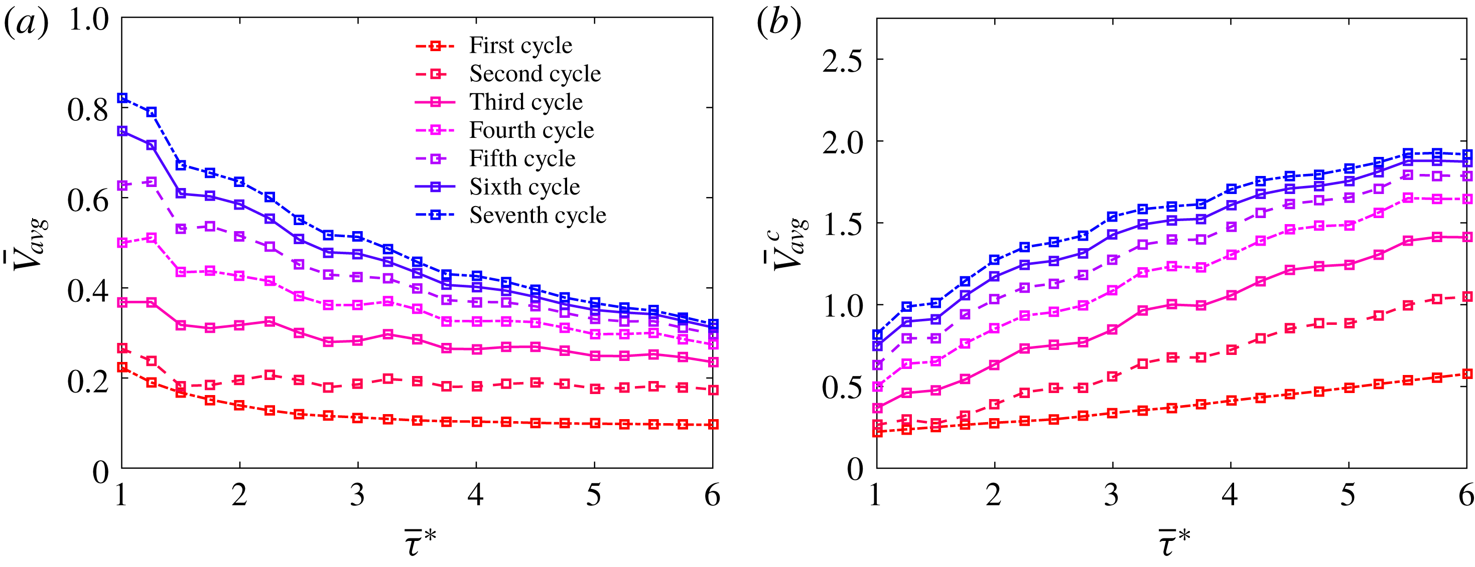
. When the average velocity is calculated using the distance travelled per propulsive cycle, lower frequency bells swim farther.
Driving the bell near the resonant frequency (
 $\bar{\unicode[STIX]{x1D70F}}^{\ast }=1$
) yielded higher swimming speeds over the propulsive cycle. In figure 11(a), we show
 $\bar{V}_{avg}$
as a function of
 $\bar{\unicode[STIX]{x1D70F}}$
over the seven propulsive cycles. We note that the optimal driving frequency is at the resonant frequency. Examining the performance of the bell for lower frequencies, we note that the peak
 $\bar{V}_{avg}$
shifts from a
 $\bar{\unicode[STIX]{x1D70F}}$
that is slightly longer than
 $\bar{\unicode[STIX]{x1D70F}}^{\ast }$
during the intermediate cycles before shifting to
 $\bar{\unicode[STIX]{x1D70F}}^{\ast }$
. This is possibly due to added mass effects that shift as the swimming speed increases and the boundary layer of the bell decreases. We also note the presence of a second, lower peak in
 $\bar{V}$
near
 $\bar{\unicode[STIX]{x1D70F}}=2.25$
in the intermediate cycles. In later cycles, this second peak shifts to
 $\bar{\unicode[STIX]{x1D70F}}=2.0$
and
 $1.75$
. We note that the simulations are approaching a steady state swimming speed, with less than 10 % relative difference in
 $\bar{V}_{avg}$
between the sixth and seventh propulsive cycle.
Plots of the out-of-plane vorticity,
 $\bar{\unicode[STIX]{x1D714}}_{y}$
at
 $\bar{t}^{c}=4.0$
for bells with
 $\bar{\unicode[STIX]{x1D702}}=\bar{\unicode[STIX]{x1D702}}_{ref}$
and
 $\bar{\unicode[STIX]{x1D70F}}=$
(a) 1.0, (b) 2.0, (c) 3.0, (d) 4.0, (e) 5.0 and (f) 6.0.

Plots of the vertical velocity,
 $\bar{u}_{z}$
at
 $\bar{t}=4.0$
for bells with
 $\bar{\unicode[STIX]{x1D702}}=\bar{\unicode[STIX]{x1D702}}_{ref}$
and
 $\bar{\unicode[STIX]{x1D70F}}=$
(a) 1.0, (b) 2.0, (c) 3.0, (d) 4.0, (e) 5.0 and (f) 6.0.

Bells with longer periods travelled farther per propulsive cycle than those with shorter periods. Plotting
 $\bar{V}_{avg}^{c}$
with respect to
 $\bar{\unicode[STIX]{x1D70F}}$
(figure 11
b), we generally find that
 $\bar{V}_{avg}^{c}$
increases as
 $\bar{\unicode[STIX]{x1D70F}}$
increases, with
 $\bar{V}_{avg}^{c}$
plateauing for
 $\bar{\unicode[STIX]{x1D70F}}\geqslant 5.5$
at later cycles. Recall that
 $\bar{V}_{avg}^{c}$
describes the bell heights travelled per propulsive cycle. This illustrates the role of the stopping vortex ring in generating forward movement after the expansion phase. As the
 $\bar{\unicode[STIX]{x1D70F}}^{\ast }$
increases, the passive energy recapture due to the stopping vortex ring continues to propel the bell forward for no additional energy cost. For
 $\bar{\unicode[STIX]{x1D70F}}\geqslant 5.5$
, the additional distance travelled due to the stopping vortex ring does not increase relative to the distance travelled for bells with shorter periods.
Plots of the stopping vortex ring circulation,
 $\bar{\unicode[STIX]{x1D6E4}}$
, with respect to
 $\bar{\unicode[STIX]{x1D70F}}$
at
 $\bar{t}^{c}=7.0$
for a bell with
 $\bar{\unicode[STIX]{x1D702}}=\bar{\unicode[STIX]{x1D702}}_{ref}$
.

(a) Plot of
 $\bar{A}_{z}$
with respect to
 $\bar{t}$
from
 $36$
to
 $42$
for a bell of
 $\bar{\unicode[STIX]{x1D702}}=\bar{\unicode[STIX]{x1D702}}_{ref}$
driven at
 $\bar{\unicode[STIX]{x1D70F}}=6.0$
. (b) The average of the
 $\bar{A}_{z}$
,
 $\bar{A}_{avg}$
, over different intervals of the final propulsive cycle for a bell of
 $\bar{\unicode[STIX]{x1D702}}=\bar{\unicode[STIX]{x1D702}}_{ref}$
driven at
 $\bar{\unicode[STIX]{x1D70F}}=6.0$
.

As the period of the propulsive cycle increases, the distance between the starting and stopping vortex rings increases as well. In figure 12, we plot
 $\bar{\unicode[STIX]{x1D714}}_{y}$
at
 $\bar{t}=4.0$
for bells with
 $\bar{\unicode[STIX]{x1D70F}}=1.0,2.0,3.0,4.0,5.0$
and
 $6.0$
. For all cases considered, starting vortex rings are shed into the wake of the bell, and stopping vortices are observed in the subumbrellar cavity. As
 $\bar{\unicode[STIX]{x1D70F}}$
increases, the distance between the stopping and starting vortex ring increases, as does the distance between starting vortex rings from previous propulsive cycles. To illustrate these difference in the wake, we plot the instantaneous vertical flow,
 $\bar{u}_{z}$
, in the
 $xz$
-plane (figure 13). As the distance between the starting and stopping vortex ring increases, the strength of their interaction decreases, with a smaller region of positive vertical velocity present in the immediate wake. The immediate wake of the bell with
 $\bar{\unicode[STIX]{x1D70F}}=1.0$
is also affected by the starting vortex ring in the third propulsive cycle.
To quantify the strength of the stopping vortex ring, its dimensionless circulation,
 $\bar{\unicode[STIX]{x1D6E4}}$
, was calculated at the end of the bells’ seventh propulsive cycle (
 $\bar{t}^{c}=7.0$
). In figure 14, we show
 $\bar{\unicode[STIX]{x1D6E4}}$
as a function of
 $\bar{\unicode[STIX]{x1D70F}}$
. An initial peak in circulation is present at
 $\bar{\unicode[STIX]{x1D70F}}=1.0$
, which is followed by a steep decline to a plateau where the circulation remains nearly constant from
 $\bar{\unicode[STIX]{x1D70F}}=1.5$
to
 $3.25$
. After this point, the circulation decreases at a higher rate. This suggests that there is a limit to the additional thrust generated by the stopping vortex rings due to viscous dissipation.
To further examine the role of the stopping vortex in driving the bell forward, we calculated the vertical acceleration,
 $\bar{A}_{z}=(\unicode[STIX]{x2202}\bar{V}_{z}/\unicode[STIX]{x2202}\bar{t})$
, of the bell for
 $\bar{\unicode[STIX]{x1D702}}=\bar{\unicode[STIX]{x1D702}}_{ref}$
driven at
 $\bar{\unicode[STIX]{x1D70F}}=6.0$
(figure 15
a). If the bell was moving forward solely due to the inertia from the contraction phase, then the bell should have be averaging a negative acceleration during the coasting phase due to the drag on the bell. In figure 15(b) we plot the average
 $\bar{A}_{z}$
of the bell,
 $\bar{A}_{avg}$
, over
 $\bar{t}=2.0$
length intervals for the final propulsive cycle. We note that the average acceleration over in the first interval, which includes both the contraction and expansion of the bell, is positive. In the second interval, during which the bell is already fully expanded and being driven by the stopping vortex, is positive as well. As the strength of the stopping vortex decreases, as noted in figure 14, the drag on the bell contributes to a negative acceleration. The positive acceleration of the second interval suggests that the stopping vortex plays a significant in driving the bell forward following the contraction and expansion of the bell.
3.2.1 Varying bell stiffness
Plot of (a)
 $\bar{V}$
and (b)
 $\bar{V}^{top}$
with respect to
 $\bar{t}$
for three bells with
 $\bar{\unicode[STIX]{x1D702}}=$
 $(1/3)\bar{\unicode[STIX]{x1D702}}_{ref}$
,
 $\bar{\unicode[STIX]{x1D702}}_{ref}$
and
 $(5/3)\bar{\unicode[STIX]{x1D702}}_{ref}$
. The bell’s propulsive cycle has a period of
 $\bar{\unicode[STIX]{x1D70F}}=2.5$
. Note that
 $\bar{V}$
is the dimensionless velocity averaged over the entire bell and
 $\bar{V}^{top}$
is the dimensionless velocity associated with the bell apex. As the
 $\bar{\unicode[STIX]{x1D702}}$
is varied, the passive elastic response of the bell varies as well.

Plot of (a)
 $\bar{V}_{avg}$
and (b)
 $\bar{V}_{avg}^{c}$
with respect to
 $\bar{\unicode[STIX]{x1D70F}}^{\ast }$
for bells with
 $\bar{\unicode[STIX]{x1D702}}=(1/3)\bar{\unicode[STIX]{x1D702}}_{ref}$
,
 $\bar{\unicode[STIX]{x1D702}}_{ref}$
, and
 $(5/3)\bar{\unicode[STIX]{x1D702}}_{ref}$
. Note that
 $\bar{\unicode[STIX]{x1D70F}}\ast =1$
corresponds to the natural frequency of each of the bells.
 $\bar{V}_{avg}$
denotes the dimensionless swimming speed with respect to absolute time.
 $\bar{V}_{avg}^{c}$
denotes the average dimensionless swimming speed calculated using distance travelled per propulsive cycle. Hence, (b) shows that bells with longer driving periods swim farther per propulsive cycle.

Plot of
 $\bar{\unicode[STIX]{x1D714}}_{y}$
for bells with
 $\bar{\unicode[STIX]{x1D70F}}=0.5$
at
 $\bar{t}=7.0$
for
 $\bar{\unicode[STIX]{x1D702}}$
equal to (a)
 $(1/3)\bar{\unicode[STIX]{x1D702}}_{ref}$
, (b)
 $(2/3)\bar{\unicode[STIX]{x1D702}}_{ref}$
and (c)
 $\bar{\unicode[STIX]{x1D702}}_{ref}$
. The bell in (a) has not fully expanded at the end of its propulsive cycle, and does not form the defined starting vortex rings as found in the wakes of (b) and (c). The bell in (a) lacks the large region of positive
 $\bar{u}$
found in (b) and (c). Note that the bell in (a) is driven faster than its resonant frequency, while the bell in (c) is being driven at its resonant frequency. The bell in (b) is being slightly faster than its resonant frequency (
 $\bar{\unicode[STIX]{x1D70F}}^{\ast }=0.8$
) but is allowed enough time to expand. See supplementary movie 2.

Plot of
 $\bar{u}_{z}$
on the
 $xz$
-plane for bells with
 $\bar{\unicode[STIX]{x1D70F}}=0.5$
at
 $\bar{t}=7.0$
for
 $\bar{\unicode[STIX]{x1D702}}$
equal to (a)
 $(1/3)\bar{\unicode[STIX]{x1D702}}_{ref}$
, (b)
 $(2/3)\bar{\unicode[STIX]{x1D702}}_{ref}$
, (c)
 $\bar{\unicode[STIX]{x1D702}}_{ref}$
. The bell in (a) lacks the large region of positive
 $\bar{u}$
found in (b) and (c). Note that the bell in (a) is driven faster than its resonant frequency, while the bell in (c) is being driven at its resonant frequency. The bell in (b) is being slightly faster than its resonant frequency (
 $\bar{\unicode[STIX]{x1D70F}}^{\ast }=0.8$
) but still performs well.

Plot of (a) average input power (
 $\bar{P}_{avg}$
), (b) swimming economy (
 $\unicode[STIX]{x1D700}$
) and (c) cost of transport (COT) with respect to
 $\bar{\unicode[STIX]{x1D70F}}^{\ast }$
for bells with
 $\bar{\unicode[STIX]{x1D702}}=(1/3)\bar{\unicode[STIX]{x1D702}}_{ref}$
,
 $\bar{\unicode[STIX]{x1D702}}_{ref}$
and
 $(5/3)\bar{\unicode[STIX]{x1D702}}_{ref}$
. Recall that the bells are driven at their resonant frequency when
 $\bar{\unicode[STIX]{x1D70F}}^{\ast }=1$
.

Plot of
 $\bar{\unicode[STIX]{x1D714}}_{y}$
on the
 $xz$
-plane for bells with
 $\bar{\unicode[STIX]{x1D70F}}^{\ast }\approx 2.5$
at
 $\bar{t}^{c}=6.0$
for
 $\bar{\unicode[STIX]{x1D702}}$
equal to (a)
 $(1/3)\bar{\unicode[STIX]{x1D702}}_{ref}$
(
 $\bar{\unicode[STIX]{x1D70F}}=4.25$
), (b)
 $(1/3)\bar{\unicode[STIX]{x1D702}}_{ref}$
(
 $\bar{\unicode[STIX]{x1D70F}}=3.0$
) and (c)
 $\bar{\unicode[STIX]{x1D702}}_{ref}$
(
 $\bar{\unicode[STIX]{x1D70F}}=2.5$
), (d)
 $(4/3)\bar{\unicode[STIX]{x1D702}}_{ref}$
(
 $\bar{\unicode[STIX]{x1D70F}}=2.25$
), and (e)
 $(5/3)\bar{\unicode[STIX]{x1D702}}_{ref}$
(
 $\bar{\unicode[STIX]{x1D70F}}=2.0$
). See supplementary movie 3.

Plot of
 $\bar{u}_{z}$
on the
 $xz$
-plane for bells with
 $\bar{\unicode[STIX]{x1D70F}}^{\ast }\approx 2.5$
at
 $\bar{t}^{c}=6.0$
for
 $\bar{\unicode[STIX]{x1D702}}$
equal to (a)
 $(1/3)\bar{\unicode[STIX]{x1D702}}_{ref}$
(
 $\bar{\unicode[STIX]{x1D70F}}=4.25$
), (b)
 $(1/3)\bar{\unicode[STIX]{x1D702}}_{ref}$
(
 $\bar{\unicode[STIX]{x1D70F}}=3.0$
), (c)
 $\bar{\unicode[STIX]{x1D702}}_{ref}$
(
 $\bar{\unicode[STIX]{x1D70F}}=2.5$
), (d)
 $(4/3)\bar{\unicode[STIX]{x1D702}}_{ref}$
(
 $\bar{\unicode[STIX]{x1D70F}}=2.25$
) and (e)
 $(5/3)\bar{\unicode[STIX]{x1D702}}_{ref}$
(
 $\bar{\unicode[STIX]{x1D70F}}=2.0$
).

Plot of the dimensionless stopping vortex ring circulation,
 $\bar{\unicode[STIX]{x1D6E4}}$
, versus the normalized elastic modulus of the bell,
 $\bar{\unicode[STIX]{x1D702}}/\bar{\unicode[STIX]{x1D702}}_{ref}$
, for five bells with
 $\bar{\unicode[STIX]{x1D70F}}^{\ast }\approx 2.5$
at
 $\bar{t}^{c}=7.0$
.

To further examine the role of resonance, we varied the bell’s elastic modulus (see table 1) and varied the driving frequency. In figure 16(a), we plot
 $\bar{V}^{top}$
with respect to
 $\bar{t}$
for three bells of with elastic moduli of
 $(1/3)\bar{\unicode[STIX]{x1D702}}_{ref},\bar{\unicode[STIX]{x1D702}}_{ref}$
and
 $(5/3)\bar{\unicode[STIX]{x1D702}}_{ref}$
, and a propulsive cycle of length
 $\bar{\unicode[STIX]{x1D70F}}=2.5$
. We remind that
 $\bar{V}$
is non-dimensionalized with respect to the bell’s period of free vibration,
 $\unicode[STIX]{x1D70F}^{\ast }$
, and that it is averaged over the entire bell. We find that
 $\bar{V}$
for all three bells display oscillations in the forward swimming speed, as seen in figure 9(a), but that the frequency of those oscillations varies as a function of
 $\bar{\unicode[STIX]{x1D702}}$
, with higher frequency oscillations occurring for the stiffest bell (
 $(5/3)\bar{\unicode[STIX]{x1D702}}_{ref}$
) and lower frequency oscillations for the most flexible bell (
 $(1/3)\bar{\unicode[STIX]{x1D702}}_{ref}$
). We also note that the point at which peak
 $\bar{V}$
occurs shifts to later in the propulsive cycle as
 $\bar{\unicode[STIX]{x1D702}}$
decreases.
Plotting
 $\bar{V}_{avg}$
of the seventh propulsive cycle with respect to the effective period,
 $\bar{\unicode[STIX]{x1D70F}}^{\ast }$
, we find that the bell swims fastest when the propulsive cycle is equal to its period of free vibration (
 $\bar{\unicode[STIX]{x1D70F}}^{\ast }=1.0$
) or slightly less than it. If the period is too short, as seen for the first point of the
 $(1/3)\bar{\unicode[STIX]{x1D702}}_{ref}$
curve, the bell does not produce significant forward swimming speed. For
 $\bar{\unicode[STIX]{x1D70F}}^{\ast }>1.0$
we see a steady decline in
 $\bar{V}_{avg}$
, as previously observed in figure 11(b). Examining
 $\bar{V}_{avg}^{c}$
in figure 17(b), we find that longer
 $\bar{\unicode[STIX]{x1D70F}}^{\ast }$
travel farther per cycle, but
 $\bar{V}_{avg}^{c}$
levels off at earlier
 $\bar{\unicode[STIX]{x1D70F}}^{\ast }$
when
 $\bar{\unicode[STIX]{x1D702}}$
is lower.
To further examine the role of resonance, we show the out-of-plane vorticity,
 $\bar{\unicode[STIX]{x1D714}}_{y}$
, for three bells with the elastic modulus set to
 $(1/3)\bar{\unicode[STIX]{x1D702}}_{ref},(2/3)\bar{\unicode[STIX]{x1D702}}_{ref}$
and
 $\bar{\unicode[STIX]{x1D702}}$
driven with a propulsive cycle period of
 $\bar{\unicode[STIX]{x1D70F}}=1.0$
(figure 18). The most flexible case (
 $(1/3)\bar{\unicode[STIX]{x1D702}}_{ref}$
) is driven above its resonant frequency, and is not given enough time during the propulsive cycle to expand fully to its resting state. As such the bell is not fully expanded by the time the next propulsive cycle begin, leading to a less defined starting vortex ring. We find that the distinct separation of the starting vortex rings in the wake, as seen in the higher
 $\bar{\unicode[STIX]{x1D702}}$
cases, is absent. Also absent for the more flexible bell is the separation of the starting and stopping vortex rings in the immediate wake. Examining the vertical velocity in a 2-D plane through the central axis of the bell (figure 19), we find that the absence of this vortex ring separation yields a smaller region of positive
 $\bar{u}_{z}$
in the immediate wake. Movie 2 detailing this case is included in the supplementary materials.
To describe the efficiency as a function of the bell elastic modulus and the driving frequency, we calculated that average power input,
 $\bar{P}_{avg}$
, the swimming economy,
 $\unicode[STIX]{x1D716}$
, and the cost of transport, COT, for each of the cases.
 $\bar{P}_{avg}$
generally decreased as the effective period,
 $\bar{\unicode[STIX]{x1D70F}}^{\ast }$
, increased (figure 20
a). When the bell was driven above its natural frequency,
 $\bar{\unicode[STIX]{x1D70F}}\ast <1.0$
for
 $(1/3)\bar{\unicode[STIX]{x1D70F}}$
, the average power input was lower since less work was done as the bell did not fully expand. There was a second local peak in
 $\bar{P}_{avg}$
at
 $\bar{\unicode[STIX]{x1D70F}}^{\ast }\approx 2.25$
for all
 $\bar{\unicode[STIX]{x1D702}}$
. For fixed
 $\bar{\unicode[STIX]{x1D70F}}^{\ast }$
,
 $\bar{P}_{avg}$
was slightly higher for stiffer bells, due to this study maintaining tension magnitude in proportion to the bell’s elastic modulus. However, we note that the non-dimensionalization of
 $\bar{P}_{avg}$
collapses fairly well for the different
 $\bar{\unicode[STIX]{x1D702}}$
. Examining the swimming economy of the bell,
 $\unicode[STIX]{x1D700}$
, with respect to the effective period,
 $\bar{\unicode[STIX]{x1D70F}}^{\ast }$
, we found that the swimming economy increased as
 $\bar{\unicode[STIX]{x1D70F}}^{\ast }$
increased (figure 20
b). Local peaks in
 $\unicode[STIX]{x1D716}$
were noted at
 $\bar{\unicode[STIX]{x1D70F}}^{\ast }$
that corresponded to multiples of the period of free vibration,
 $\unicode[STIX]{x1D70F}^{\ast }$
. We also found that though the swimming economy of the bells showed relatively good agreement, the swimming economy was generally higher for more flexible bells. Similarly, more flexible bells had a lower cost of transport, COT. Increasing the pulsing cycle duration,
 $\bar{\unicode[STIX]{x1D70F}}$
, led to a decrease in COT for a given stiffness (figure 20
c).
Collapsing our results with respect to
 $\bar{\unicode[STIX]{x1D70F}}^{\ast }$
allowed us to compare bells of different stiffnesses relative to the period of free vibration. We generally find that bells driven at the same
 $\bar{\unicode[STIX]{x1D70F}}^{\ast }$
have similar
 $\bar{V}_{avg}$
and
 $\bar{V}_{avg}^{c}$
, with the exception being the most flexible case,
 $(1/3)\bar{\unicode[STIX]{x1D702}}_{ref}$
, which swims at a slightly slower speed. Plotting the vorticity associated with bells of
 $\bar{\unicode[STIX]{x1D70F}}^{\ast }\approx 2.5$
(figure 21), we find similarity in the vorticity profiles of the bells. Note that the bells are driven at different frequencies. Plotting
 $\bar{u}_{z}$
on the
 $xz$
-place for the bells reveal similarities in the immediate wake of the bell. In that region, positive
 $\bar{u}_{z}$
is present due to the starting and stopping vortex ring interactions (figure 22). However, we note that as
 $\bar{\unicode[STIX]{x1D702}}$
decreases, the similarity in swimming speeds decreases. This is a result of the limitations in the relative strength of applied tension in overcoming the fluid forces associated with pushing fluid out of the bell, as had been previously noted in Hoover & Miller (Reference Hoover and Miller2015). As the stiffness of the bell increases, the relative difference between bells of similar
 $\bar{\unicode[STIX]{x1D70F}}^{\ast }$
decreases. Calculating the dimensionless circulation at
 $\bar{t}^{c}=7.0$
for the five bells of figures 21 and 22, we find that the circulation of the stopping vortex ring remains fairly consistent across the five bells of varying
 $\bar{\unicode[STIX]{x1D702}}$
and
 $\bar{\unicode[STIX]{x1D70F}}$
. Movie 3 detailing this case is included in the supplementary materials.
3.3 Short time scale study
Short time scale study parameters.

(a) Plot of the temporal parametrization of the activation and release of muscular tension,
 $\unicode[STIX]{x1D6FC}$
, for the short time scale study for
 $\bar{\unicode[STIX]{x1D70F}}=0.5,$
 $1.0$
and
 $1.5$
. (b) Plot of
 $\bar{V}$
with respect to
 $\bar{t}$
for the short time scale study using the
 $\unicode[STIX]{x1D6FC}$
of (a).

Plots of (a)
 $\bar{V}_{avg}$
, (b)
 $\bar{V}_{avg}^{c}$
and (c)
 $\bar{P}_{avg}$
with respect to
 $\bar{\unicode[STIX]{x1D70F}}^{\ast }$
for bells with
 $\bar{\unicode[STIX]{x1D702}}=(1/3)\bar{\unicode[STIX]{x1D702}}_{ref}$
,
 $\bar{\unicode[STIX]{x1D702}}_{ref}$
and
 $(5/3)\bar{\unicode[STIX]{x1D702}}_{ref}$
for the short time scale
 $\unicode[STIX]{x1D6FC}$
. We note that
 $\bar{P}_{avg}$
peaks at
 $0.6<\bar{\unicode[STIX]{x1D70F}}^{\ast }<1.0$
and decreases as
 $\bar{\unicode[STIX]{x1D70F}}^{\ast }$
increases as it did for the case in § 3.2. However, we note a low
 $\bar{P}_{avg}$
for
 $\bar{\unicode[STIX]{x1D70F}}^{\ast }<0.6$
due to the bell not fully expanding, which in turn leads to a lower
 $\bar{V}_{rad}$
.

Due to the choice of
 $t_{len}$
,
 $\unicode[STIX]{x1D703}_{a}$
and
 $\unicode[STIX]{x1D703}_{r}$
in the temporal activation function,
 $\unicode[STIX]{x1D6FC}$
, the studies in § 3.2 are unable to fully span the parameter space of
 $\bar{\unicode[STIX]{x1D70F}}^{\ast }<1.0$
. In order to understand the role of pumping above the resonant frequency, a short time scale study is performed with a modified
 $\unicode[STIX]{x1D6FC}$
with
 $t_{len}$
,
 $\unicode[STIX]{x1D703}_{a}$
and
 $\unicode[STIX]{x1D703}_{r}$
values that allow for a shorter period of activation (see table 4). With this modified
 $\unicode[STIX]{x1D6FC}$
, the bell is driven with a range of
 $\bar{\unicode[STIX]{x1D70F}}$
equal to
 $0.5$
,
 $0.75$
,
 $1.0$
,
 $1.25$
and
 $1.5$
. In figure 24 we plot
 $\unicode[STIX]{x1D6FC}$
and the corresponding forward swimming velocity
 $\bar{V}$
for
 $\bar{\unicode[STIX]{x1D70F}}$
 $=0.5$
,
 $1.0$
and
 $1.5$
and
 $\bar{\unicode[STIX]{x1D702}}=\bar{\unicode[STIX]{x1D702}}_{ref}$
. We note the differences in the velocity profiles, where
 $\bar{\unicode[STIX]{x1D70F}}=0.5$
yields a swimming speed that does not experience the peak swimming speeds of the bells that are driven at
 $\bar{\unicode[STIX]{x1D70F}}=1.0$
and
 $1.5$
.
This range of
 $\bar{\unicode[STIX]{x1D70F}}$
allows us to examine the role of driving for
 $\bar{\unicode[STIX]{x1D70F}}^{\ast }<1.0$
for bells with
 $\bar{\unicode[STIX]{x1D702}}$
equal to
 $(1/3)\bar{\unicode[STIX]{x1D702}}_{ref}$
,
 $(2/3)\bar{\unicode[STIX]{x1D702}}_{ref}$
,
 $\bar{\unicode[STIX]{x1D702}}_{ref}$
,
 $(4/3)\bar{\unicode[STIX]{x1D702}}_{ref}$
and
 $(5/3)\bar{\unicode[STIX]{x1D702}}_{ref}$
. In figure 25(a,b), we have plotted the resulting
 $\bar{V}_{avg}$
and
 $\bar{V}_{avg}^{c}$
with respect to the resulting
 $\bar{\unicode[STIX]{x1D70F}}^{\ast }$
of the bells when driving the bell with
 $\bar{\unicode[STIX]{x1D70F}}=0.5$
,
 $0.75$
,
 $1.0$
,
 $1.25$
and
 $1.5$
. For all bells driven at
 $\bar{\unicode[STIX]{x1D70F}}^{\ast }<0.5$
, the resulting swimming speed decreases. Generally, the peaks in swimming speed occur at a range of
 $0.6<\bar{\unicode[STIX]{x1D70F}}^{\ast }<1.0$
, where stiffer bells have peaks closer to the natural period of free vibration (
 $\bar{\unicode[STIX]{x1D70F}}^{\ast }=1.0$
) whereas more flexible bells have peaks in swimming speeds of a shorter period. Examining
 $\bar{P}_{avg}$
(figure 25
c), we found that power was maximized around
 $0.6<\bar{\unicode[STIX]{x1D70F}}^{\ast }<1.0$
. As
 $\bar{\unicode[STIX]{x1D70F}}^{\ast }$
decreases,
 $\bar{P}_{avg}$
decreases as a result of the bell not fully expanding to its equilibrium state when no tension is acting on it. This in turn yields a lower
 $V_{rad}$
since it takes the bell is already near its contracted equilibrium state.
4 Discussion
Our three-dimensional numerical study of resonant driving and passive energy recapture in oblate jellyfish bells indicates that the ideal driving frequency for a given bell depends upon the metric that is to be optimized. For a given bell shape and elastic modulus with a fixed magnitude and duration of applied muscular tension, the fastest forward swimming speeds are generated when the bell is driven near its resonant frequency. If the bell is driven above this frequency, it will not fully expand before the next active contraction. This results in lower amplitude oscillations and weaker starting and stopping vortex rings that are not efficiently shed into the wake. If the bell is driven below this frequency, the average distance travelled per unit time decreases, due in part to the fact that the contractions happen less frequently. On the other hand, long coasting periods between active contractions (corresponding to lower driving frequencies) result in more efficient swimming when one considers the cost of transport and average power input. The bell is passively propelled forward for longer periods of time due to its interaction with the stopping vortex ring, though there are limits to this secondary thrust mechanism due to viscous dissipation of the stopping vortex ring. Furthermore, we have found limitations in increasing driving frequency significantly above the resonant frequency.
Our results complement but also expand our understanding of resonant swimming in jellyfish relative to previous work. The lumped parameter models by Demont & Gosline (Reference Demont and Gosline1988) and Megill (Reference Megill2002) showed that the fastest forward swimming speeds are obtained when the bell is driven at its resonant frequency. These works did not, however, show that lower frequencies lead to more efficient swimming as the models did not consider unsteady effects of the fluid or vortex–bell interactions. Hoover & Miller (Reference Hoover and Miller2015) found that for two-dimensional prolate bells, both swimming speed and cost of transport were maximized when the bell was driven near its resonant frequency. Given the prolate bell geometry and the two-dimensionality of the simulations, passive energy recapture did not have a significant effect. In our three-dimensional simulations of oblate bells, the jellyfish can coast for extended periods of time through passive energy recapture. While the average swimming speeds are slower, efficiency of movement is higher. Other differences between our results and previous models may also be due to the way in which muscular forces are applied. In earlier resonant studies, these forces are given as sinusoidal functions such that the duration of applied tension changes with driving frequency. There is also an active force during expansion that acts to re-expand the bell. By keeping the duration of applied tension constant in our model and applying no force to re-expand the bell, we note that our model of muscular tension is more representative of true jellyfish. We also comment that though the model extended muscular activation to the bell margin, the resulting fluid dynamics remains similar to the experimental studies of Gemmell et al. (Reference Gemmell, Troolin, Costello, Colin and Satterlie2015b ). Further examination of the role of the flexibility of the bell margin and its kinematics is an area of future study.
This study also further illuminates the role of passive energy recapture in jellyfish locomotion. A recent experimental study by Gemmell, Colin & Costello (Reference Gemmell, Colin and Costello2018) observed that although passive energy recapture occurs throughout the jellyfish taxa, not all jellyfish take full advantage of this mechanism. In that study it was remarked that one possible reason for this discrepancy is that jellyfish that are continuously swimming want to avoid the loss of inertia associated with longer inter-pulse durations. The results from our study confirm the observation of Gemmell et al. (Reference Gemmell, Costello, Colin, Stewart, Dabiri, Tafti and Priya2013), with significantly lower
 $\bar{V}_{avg}$
for the reference bell with long
 $\bar{\unicode[STIX]{x1D70F}}$
(figure 11
a) and diminishing returns for the distance travelled by a bell over the propulsive cycle (figure 11
b). We note that the resulting steady-state or near-steady-state swimming is higher for bells with shorter
 $\bar{\unicode[STIX]{x1D70F}}$
for the reference case. Furthermore, examining the circulation of the stopping vortex (figure 14) at the end of the propulsive cycle revealed a steady decline in circulation for
 $\bar{\unicode[STIX]{x1D70F}}\geqslant 3.5$
. This suggests that, after this point, there are diminishing returns on the additional thrust from passive energy recapture due to the decline of the intensity of the stopping vortex ring. Furthermore, it is important to keep in mind that one of the main reasons oblate jellyfish swim is to circulate fluid and nutrients through their tentacles, as opposed to moving towards a specific destination (Costello & Colin Reference Costello and Colin1995; Dabiri et al.
Reference Dabiri, Colin, Katija and Costello2010; Gemmell et al.
Reference Gemmell, Costello, Colin, Stewart, Dabiri, Tafti and Priya2013). In light of this, swimming with greater efficiency, with a longer
 $\unicode[STIX]{x1D70F}^{\ast }$
, would be more important than swimming proficiently.
Comparing the swimming performance of bells with differing material properties (figure 17
a,b) further reveals the dynamics between passive energy recapture and resonant driving. Bells driven near
 $\bar{\unicode[STIX]{x1D70F}}^{\ast }=1.0$
have a higher
 $\bar{V}_{avg}$
than bells driven with a long
 $\bar{\unicode[STIX]{x1D70F}}^{\ast }$
. Bells with a longer
 $\bar{\unicode[STIX]{x1D70F}}^{\ast }$
in turn travel farther per propulsive cycle and therefore have a higher
 $\bar{V}_{avg}^{c}$
. The two most flexible bells,
 $(1/3)\unicode[STIX]{x1D702}_{ref}$
and
 $(1/3)\unicode[STIX]{x1D702}_{ref}$
, are driven at
 $\bar{\unicode[STIX]{x1D70F}}^{\ast }<1$
and reveal the dynamics of the driving the bell above its resonant frequency. Driving slightly above the resonant frequency can yield faster swimming speeds than driving at the resonant frequency, but if the frequency is too high (figures 18 and 18) the bell does not fully expand and does not fully form the starting and stopping vortex rings present in jellyfish locomotion. To further characterize the swimming performance, we examined the efficiency of the bell by examining the swimming economy,
 $\unicode[STIX]{x1D700}$
, and cost of transport, COT, of the bell. We generally found a higher swimming economy for more flexible bells (figure 20
b) and for bells that are driven at longer
 $\bar{\unicode[STIX]{x1D70F}}^{\ast }$
. We note that the swimming economy revealed that a flexible bell driven with a shorter
 $\bar{\unicode[STIX]{x1D70F}}^{\ast }$
would have the equivalent swimming economy as a stiff bell driven with a longer
 $\bar{\unicode[STIX]{x1D70F}}^{\ast }$
. Examining cost of transport (figure 20
c) we generally find that flexible bells have a lower cost of transport. Driving at the resonant frequency led to a higher average input power,
 $\bar{P}_{avg}$
, which can explain the lower efficiency associated with
 $\bar{\unicode[STIX]{x1D70F}}\approx 1.0$
. By examining the effects of driving above the resonant frequency, we found that driving the bell in the range of
 $0.6<\bar{\unicode[STIX]{x1D70F}}^{\ast }<1.0$
led to peak swimming speeds (figure 25
a,b), but a lower
 $\bar{\unicode[STIX]{x1D70F}}$
resulted in a significant decrease in swimming speed. This result further illustrates the limitations of driving above the resonant frequency.
The collapse of
 $\bar{V}_{avg}$
for bells of differing material properties using
 $\bar{\unicode[STIX]{x1D70F}}^{\ast }$
also reveals the interplay between the material properties of the structure and the fluid motion it generates. Using the period of free vibration,
 $\unicode[STIX]{x1D70F}^{\ast }$
, as the characteristic time for
 $\bar{V}$
, we find that for bells with
 $\bar{\unicode[STIX]{x1D702}}\geqslant (2/3)\bar{\unicode[STIX]{x1D702}}_{ref}$
the resulting swimming performance is dependent on the speed of the bell’s expansion. Stiffer bells have a lower
 $\unicode[STIX]{x1D70F}^{\ast }$
and the bell will expand more quickly to its resting configuration. During this expansion, the strength of the stopping vortex ring formed will be dependent on the speed of expansion, with a higher transfer of momentum for lower
 $\unicode[STIX]{x1D70F}^{\ast }$
. Since passive energy recapture is dependent on the strength of the stopping vortex, scaling
 $\bar{\unicode[STIX]{x1D70F}}^{\ast }$
with
 $\unicode[STIX]{x1D70F}^{\ast }$
, we find that bells of similar
 $\bar{\unicode[STIX]{x1D70F}}^{\ast }$
have a similar velocity and displacement, even with differences in the driving frequency (figures 21 and 22). This further elucidates the relationship between the bell’s material properties and the fluid forces the bell generates. This relationship was also examined in Hoover et al. (Reference Hoover, Griffith and Miller2017), where the speed of the starting vortex rings was found to be dependent on the strength of the applied active tension. However, the length of the propulsive cycle was held fixed in that study and the effects that the material properties have on passive energy recapture were not fully examined. The results from our study further explain how these material properties affect the strength of the starting and stopping vortex rings and their role in both resonant driving and passive energy recapture.
Acknowledgements
We would like to thank R. Cortez, L. Fauci and B. Griffith for their advice and insights throughout this research project. This research was funded by a National Science Foundation (NSF) DMS CAREER no. 1151478 (to L.A.M.). A.J.P. was supported with the University of North Carolina at Chapel Hill’s Summer Undergraduate Research Fellowship. We also thank G. McLaughlin, who took the Aurelia spp. photo in figure 1. All other images were generated in Matlab and VisIt.
Supplementary materials
Supplementary materials are available at https://doi.org/10.1017/jfm.2018.1007.



