


1 INTRODUCTION
Penalization is a standard device in econometrics and statistics for stabilizing estimation, shrinking nuisance components, and enforcing low-dimensional structure such as sparsity; classical examples include Ridge, Lasso, SCAD, and related procedures in least-squares and likelihood settings (Hoerl and Kennard, Reference Hoerl and Kennard1970; Tibshirani, Reference Tibshirani1996; Fan and Li, Reference Fan and Li2001; Yuan and Lin, Reference Yuan and Lin2006). The usual approach is to append a penalty directly to the criterion that defines the estimator of interest, as in penalized least squares, penalized likelihood, or penalized GMM (Green, Reference Green1987; Frank and Friedman, Reference Frank and Friedman1993; Caner, Reference Caner2009). That approach is natural and often effective, but it also ties regularization to the specific global geometry of the criterion being optimized. As a consequence, existence, uniqueness, finite-sample stability, and asymptotic behavior typically have to be established for each penalized problem in a model- and criterion-specific way.
This article develops a different approach. Instead of regularizing by modifying the original criterion, we start from a benchmark estimator and then define a penalized estimator by applying a single proximal regularization step to it. Throughout the article, the parameter dimension p is fixed. Given a benchmark estimator
$\hat {\boldsymbol {\beta }}_n^s\in {\mathbb {R}}^p$
 , a symmetric positive definite matrix
$\boldsymbol {W}_n$
 , a convex penalty function
$f_n$
 , and a tuning parameter
$\lambda _n>0$
 , we consider estimators of the form

where
$\|\boldsymbol {v}\|_{\boldsymbol {W}_n}^2:=\boldsymbol {v}'\boldsymbol {W}_n \boldsymbol {v}$
 . We call
$\hat {\boldsymbol {\beta }}_n$
 a proximal estimator. In this construction,
$\hat {\boldsymbol {\beta }}_n^s$
 carries the model-specific statistical content,
$\boldsymbol {W}_n$
 determines the local geometry of the regularization step, and
$f_n$
 determines the form of shrinkage, selection, or constraint enforcement.
The point of view in (1) is not meant to replace penalize-the-criterion methods. Rather, it provides a complementary and modular formulation of regularization. The benchmark step and the regularization step are separated. Once
$\hat {\boldsymbol {\beta }}_n^s$
 is available, the proximal step is a strongly convex optimization problem under the sole requirement
$\boldsymbol {W}_n\succ \boldsymbol {0}$
 and is therefore globally well posed. This separation turns out to be particularly useful. It first produces desirable finite-sample regularity properties independently of the choice of benchmark estimator
$\hat {\boldsymbol {\beta }}_n^s$
 . Second, it enables a unified asymptotic analysis for the regularized estimator, which seamlessly combines the limit law of the benchmark with the local geometry of the penalty. In this sense, the proximal route isolates regularization from the model-specific geometry of the benchmark problem while preserving a transparent link between the two.
The connection with familiar penalized estimators is immediate in regular linear models. When the benchmark is least squares and the proximal metric is chosen to be the sample design matrix, the proximal step reproduces the usual convex penalized least-squares estimator (PLSE). Thus, in standard settings, the proximal formulation does not create an unrelated class of procedures; it recovers familiar estimators from a different angle. At the same time, the same construction remains meaningful well beyond least squares. For instance, in nonlinear or multi-step problems such as two-step GMM, one may regularize an econometrically natural benchmark estimator without altering the original criterion, and hence without coupling the nonsmooth penalty to the full nonlinear objective. This distinction is especially useful when one wants regularization to inherit the benchmark’s local geometry while keeping the regularization step globally well-defined.
The article develops a general convex-analysis framework for estimators of the form (1). Our first contribution is to establish their finite-sample properties. We show that proximal estimators are always uniquely defined under a positive definite metric, satisfy deterministic stability bounds, and admit equivalent primal and dual characterizations based on convex conjugacy. For sublinear penalties, the dual characterization reduces to a projection–residual decomposition onto a closed convex set. This geometry yields a transparent interpretation of shrinkage and selection and shows that familiar formulas, such as soft-thresholding for Lasso-type procedures under orthonormal designs, are special cases of a more general projection structure.
Our second contribution is asymptotic. We derive a general limit theory for proximal estimators under a high-level assumption on the benchmark estimator and mild regularity conditions on the metric and the penalty sequence. All these asymptotic results are derived in the classical large-n, fixed-p regime. The resulting limit distributions are characterized in closed form by three objects only: the asymptotic distribution of the benchmark estimator, the local limit geometry of the penalty, and the limiting metric of the proximal step. This framework nests classical asymptotic results for convex PLSEs, including the benchmark results of Knight and Fu (Reference Knight and Fu2000), but it also applies in settings where the benchmark is not least squares and where penalize-the-criterion analyses require a dedicated local expansion of the penalized objective. We further derive oracle results, in the sense of Fan and Li (Reference Fan and Li2001), for proximal estimators. The conditions are formulated directly in terms of the local behavior of the penalty along active and inactive coordinates and are therefore easy to verify for standard examples. A useful implication is that the benchmark estimator and the penalty play conceptually distinct roles: the former supplies the local stochastic limit, while the latter determines whether shrinkage produces consistent selection and oracle-type asymptotic behavior.
These asymptotic and oracle results are especially transparent in dual form. Through Moreau decomposition, the proximal step can be written as the benchmark estimator minus a dual correction determined by the conjugate penalty; for sublinear penalties, this correction is a projection onto a closed convex set. This viewpoint isolates the mechanism through which selection occurs. Exact zeros arise through dual feasibility: oracle selection fails when the dual correction cannot absorb the inactive benchmark fluctuation, and it holds when the local subdifferential geometry generates sufficient separation on inactive coordinates. In this sense, the dual formulation turns support recovery and oracle efficiency into geometric questions about projections, dual sets, and local subgradients, rather than penalty-specific algebra.
Our third contribution concerns linear regression under irregular designs, by which we mean that the population design matrix may be singular and the sample design may either inherit this singularity or approach it asymptotically. This is the setting in which the proximal formulation is particularly useful. Under a regular design, least squares and the corresponding PLSEs are well behaved. Under a singular or nearly-singular design, by contrast, the population normal equations need not identify a unique coefficient vector, and standard least-squares-type estimators may exhibit a slower convergence rate, or otherwise nonstandard first-order behavior. For bridge-type PLSEs under nearly-singular designs, slower rates and nonstandard limits are documented in Knight and Fu (Reference Knight and Fu2000) and Knight (Reference Knight2008). Related irregularity also affects GMM and GEL procedures, as shown by Caner (Reference Caner2008), and more broadly motivates singularity-robust inference in moment condition models (see Andrews and Guggenberger, Reference Andrews and Guggenberger2019).
A central point, emphasized throughout our analysis, is that when the population design is singular, the coefficient vector of the linear model is generally not point identified. Accordingly, the article does not claim regular inference for an unidentified coefficient vector. Instead, in the irregular-design problem, we target the Ridgeless estimand, defined as the unique minimizer of the limiting population least-squares criterion over the range of the limit design matrix. By eliminating the unidentified kernel component, this target is the unique least-squares representative determined by the limiting least-squares objects alone and, among linear selections from the identified set, the unique one compatible with
$\sqrt n$
 -regular inference without an auxiliary normalization.
Building on this target, we construct a new modified Ridgeless benchmark estimator based on a rank-consistent estimate of the population design matrix. This estimator is
$\sqrt n$
 -consistent and asymptotically normal for the Ridgeless target under regular, singular, and nearly-singular designs. Applying suitable proximal penalties to this benchmark then yields penalized estimators that remain well behaved across all three regimes and, under suitable adaptive penalties, can satisfy the oracle property of Fan and Li (Reference Fan and Li2001).
The article therefore has two intertwined messages. At a general level, it shows that a single proximal step applied to a benchmark estimator yields a tractable and flexible framework for penalized estimation and inference. At an applied theoretical level, it shows that this modular route is powerful enough to address a concrete problem in linear regression with irregular designs: one first stabilizes the benchmark estimator for a meaningful and identified least-squares target, and then introduces shrinkage through a proximal penalty while preserving a transparent first-order theory.
The remainder of the article is organized as follows. Section 2 develops the proximal framework, relates it to penalized least squares, and introduces the basic properties that drive the subsequent analysis. Section 3 derives the asymptotic distributions and oracle properties of proximal estimators. Section 4 applies the general theory to linear regression under regular, singular, and nearly-singular designs, by introducing the modified Ridgeless benchmark and the associated oracle proximal estimators. The convex-analysis background, supporting results, Monte Carlo analysis, and proofs are provided in the Supplementary Material.
2 PROXIMAL ESTIMATION FRAMEWORK
Throughout the article, n and p denote positive integers, with p fixed across the asymptotic analysis. Real-valued vectors are written in boldface, for example,
$\boldsymbol {x},\boldsymbol {y},\boldsymbol {\beta }$
 , and real-valued matrices in bold capitals, for example,
$\boldsymbol {X},\boldsymbol {W},\boldsymbol {Q}$
 . All random elements are defined on a complete probability space
$(\Omega ,\mathcal F,\Pr )$
 , and all stochastic convergences are understood with respect to
$\Pr $
 . We use standard notation from convex analysis, summarized in Section A.1 of the Supplementary Material.
Let
$\Gamma ({\mathbb {R}}^p)$
 denote the class of proper, lower semicontinuous, convex functions from
${\mathbb {R}}^p$
 to
$(-\infty ,+\infty ]$
 .Footnote
1
Throughout the article, a proximal estimator is an estimator of the form (1), based on a benchmark estimator
$\hat {\boldsymbol {\beta }}_n^s\in {\mathbb {R}}^p$
 , a penalty
$f_n\in \Gamma ({\mathbb {R}}^p)$
 , a tuning parameter
$\lambda _n>0$
 , and a symmetric weight matrix
$\boldsymbol {W}_n\succ \boldsymbol {0}$
 . Equivalently,

where, for each
$\boldsymbol {\theta }\in {\mathbb {R}}^p$
 ,

denotes the proximal operator of
$\lambda _n f_n$
 with respect to the inner product
$\langle \cdot ,\cdot \rangle _{\boldsymbol {W}_n}$
 .Footnote
2
This section relates the construction to penalized least squares, illustrates its use beyond linear models, and introduces basic properties that will play a central role in the sequel.
2.1 Link to Penalized Least Squares
We begin with linear regression, where the proximal construction can be compared directly with familiar PLSEs. Consider the model

where
$\boldsymbol {X}\in {\mathbb {R}}^{n\times p}$
 is a possibly random design matrix and
$\boldsymbol {\varepsilon }\in {\mathbb {R}}^n$
 is an error vector. Given
$\lambda _n>0$
 and
$f_n:{\mathbb {R}}^p\to (-\infty ,+\infty ]$
 , define the associated PLSE by

This class includes many penalties from the literature: Ridge, Lasso, Adaptive Lasso, Group Lasso, Elastic Net, and indicator penalties corresponding to constrained least squares. We refer to these as our benchmark penalties and define them in Section B.1 of the Supplementary Material.
When
$f_n\in \Gamma ({\mathbb {R}}^p)$
 , the criterion in (5) is convex, but uniqueness need not hold under singular designs or non-strictly convex penalties. By contrast, the proximal estimator in (2) is always uniquely defined once
$\boldsymbol {W}_n\succ \boldsymbol {0}$
 . Under a regular design, the two constructions coincide exactly.
Proposition 2.1 (PLSEs as Proximal Estimators under Regular Designs).
In model (4), suppose
$\boldsymbol {Q}_n:=\boldsymbol {X}'\boldsymbol {X}/n\succ \boldsymbol {0}$
 . Fix
$\lambda _n>0$
 and
$f_n\in \Gamma ({\mathbb {R}}^p)$
 , and let

Then
$\hat {\boldsymbol {\beta }}_n^{\mathrm {plse}}$
 in (5) is unique and satisfies

Thus, under regular designs, every convex PLSE is a proximal regularization of least squares under the design metric
$\boldsymbol {Q}_n$
 . In particular, the proximal formulation is not an alternative to familiar penalized least-squares procedures in such settings; it is an equivalent representation of them. When
$\boldsymbol {Q}_n$
 is singular,
$\|\cdot \|_{\boldsymbol {Q}_n}$
 is only a seminorm rather than a norm. As a result, the proximal problem may not be well defined, due to the flatness of the quadratic term along
$\operatorname {\mathrm {Kernel}}(\boldsymbol {Q}_n)$
 in equation (1). In these settings, we show that it is convenient to additionally penalize parametric directions in
$\operatorname {\mathrm {Kernel}}(\boldsymbol {Q}_n)$
 . Specifically, we consider the Ridgeless estimator (Hastie et al., Reference Hastie, Montanari, Rosset and Tibshirani2022):

where
$\boldsymbol {Q}_n^+$
 is the Moore–Penrose inverse of
$\boldsymbol {Q}_n$
 , and define

Note that since
$\boldsymbol {Q}_n\boldsymbol {Q}_n^+$
 is by construction the Euclidean orthogonal projector onto
$\operatorname {\mathrm {Range}}(\boldsymbol {Q}_n)=\operatorname {\mathrm {Range}}(\boldsymbol {X}')$
 ,
$\boldsymbol {I}_p-\boldsymbol {Q}_n\boldsymbol {Q}_n^+$
 is the Euclidean orthogonal projector onto
$\operatorname {\mathrm {Kernel}}(\boldsymbol {Q}_n)=\operatorname {\mathrm {Kernel}}(\boldsymbol {X})$
 . Hence,
$\overline {\boldsymbol {Q}}_n$
 coincides with
$\boldsymbol {Q}_n$
 on
$\operatorname {\mathrm {Range}}(\boldsymbol {Q}_n)$
 , while adding an identity component on
$\operatorname {\mathrm {Kernel}}(\boldsymbol {Q}_n)$
 , thus penalizing parametric directions in
$\operatorname {\mathrm {Kernel}}(\boldsymbol {Q}_n)$
 .
Proposition 2.2 (Ridgeless PLSE Representation of Proximal Estimators).
In model (4), let
$\boldsymbol {Q}_n:=\boldsymbol {X}'\boldsymbol {X}/n$
 , fix
$\lambda _n>0$
 and
$f_n\in \Gamma ({\mathbb {R}}^p)$
 , and define
$\hat {\boldsymbol {\beta }}_n^{\mathrm {rls}}$
 and
$\overline {\boldsymbol {Q}}_n$
 as in (7) and (8). Let

Then
$\overline {\boldsymbol {Q}}_n\succ \boldsymbol {0}$
 ,
$\overline f_n\in \Gamma ({\mathbb {R}}^p)$
 , and

Proposition 2.2 shows that singular designs can be handled by injecting curvature only along
$\operatorname {\mathrm {Kernel}}(\boldsymbol {X})$
 , that is, along directions that do not change fitted values. The quadratic adjustment in (9) is convex and acts only on observationally irrelevant directions. It therefore removes indeterminacy along
$\operatorname {\mathrm {Kernel}}(\boldsymbol {X})$
 while leaving the fitted-value component governed by the usual penalized least-squares tradeoff. When
$\boldsymbol {Q}_n\succ \boldsymbol {0}$
 , the projector
$\boldsymbol {I}_p-\boldsymbol {Q}_n\boldsymbol {Q}_n^+$
 vanishes,
$\overline {\boldsymbol {Q}}_n=\boldsymbol {Q}_n$
 ,
$\overline f_n=f_n$
 , and (10) reduces to Proposition 2.1. A general PLSE representation based on an arbitrary positive semidefinite metric is given in Section D.1 of the Supplementary Material.
2.2 Beyond Least Squares
The proximal formulation is not restricted to least squares. More generally, one may start from any econometrically natural benchmark estimator and regularize it through a separate proximal step. This distinction is especially useful in nonlinear or multi-stage problems, where penalizing the original criterion directly couples the penalty to model-specific curvature and may complicate both computation and analysis. The following example will serve as a running illustration.
Example 2.3 (Penalized Optimal Two-Step GMM in Nonlinear Moment Models).
Let
$w_i\in \mathcal W\subseteq {\mathbb {R}}^{p'}$
 denote the data,
$\boldsymbol {\theta }_0\in {\mathbb {R}}^d$
 the structural parameter, and consider moment functions

measurable in w and continuously differentiable in
$\boldsymbol {\theta }$
 . Assume the first set is correctly specified, while the second may be misspecified:

where
$\boldsymbol {\gamma }_0\in {\mathbb {R}}^k$
 is a misspecification parameter. Stack the parameters as

and define

so that
${\mathbb {E}}[m(w_i,\boldsymbol {\beta }_0)]=\boldsymbol {0}$
 . Here, sparsity of
$\boldsymbol {\gamma }_0$
 provides a convenient characterization of different levels of GMM misspecification and a natural starting point for moment selection. Let
$\bar m_n(\boldsymbol {\beta }):=n^{-1}\sum _{i=1}^n m(w_i,\boldsymbol {\beta })$
 . Efficient estimation of
$\boldsymbol {\beta }_0$
 is then obtained via the optimal two-step GMM estimator
$\hat {\boldsymbol {\beta }}_n^{\mathrm {2SGMM}}$
 , defined by

and

A standard approach in this setting, irrespective of moment selection, is to penalize the GMM criterion directly (Caner, Reference Caner2009; Liao, Reference Liao2013). In the present stacked formulation, moment selection can be achieved with an Adaptive Lasso penalty acting on the misspecification block. Given a preliminary estimator
$\tilde {\boldsymbol {\beta }}_n=(\tilde {\boldsymbol {\theta }}_n,\tilde {\boldsymbol {\gamma }}_n)$
 , defineFootnote
3
:

where
$\iota _C$
 denotes the indicator function of
$C\subseteq {\mathbb {R}}^p$
 , defined by
$\iota _C(\boldsymbol {x})=0$
 for
$x\in C$
 and
$\iota _C(\boldsymbol {x})=+\infty $
 otherwise. The corresponding penalize-the-criterion GMM estimator allowing for adaptive moment selection is

Our proximal approach instead regularizes the benchmark estimator
$\hat {\boldsymbol {\beta }}_n^{\mathrm {2SGMM}}$
 in the natural metric induced by the benchmark’s local GMM geometry. Define

If needed, one may enforce positive definiteness by replacing
$\boldsymbol {W}_n$
 with
$\boldsymbol {W}_n+\kappa _n\boldsymbol {I}_p$
 , with
$\kappa _n\downarrow 0$
 . The associated proximal GMM–Adaptive Lasso estimator is

Estimators (13) and (14) use the same adaptive weights, the same tuning parameter, and induce sparsity in the same parameter block. They differ only in how regularization enters the procedure. Indeed, the former estimator modifies the nonlinear GMM criterion itself, whereas the latter leaves the benchmark criterion unchanged and applies a single proximal step with the efficient GMM metric tied to the benchmark’s asymptotic covariance matrix. This separation between benchmark construction and regularization is the central principle underlying our approach.
2.3 Dual Representation and Projection Geometry
A useful feature of the proximal formulation is that it admits a dual characterization, and for sublinear penalties, this characterization simplifies further to a projection formula. Let
$\operatorname {\mathrm {Id}}:{\mathbb {R}}^p\to {\mathbb {R}}^p$
 denote the identity map. Given
$g\in \Gamma ({\mathbb {R}}^p)$
 , define its convex conjugate under the inner product
$\langle \cdot ,\cdot \rangle _{\boldsymbol {W}_n}$
 by

Recall that a function
$f:{\mathbb {R}}^p\to (-\infty ,+\infty ]$
 is sublinear if it is positively homogeneous and subadditive; equivalently, f is the support function of a nonempty closed convex set.
Proposition 2.4 (Dual Representation and Projection Form).
The proximal operator (3) satisfies

where
$(\lambda _n f_n)^*$
 and
$f_n^*$
 denote Fenchel conjugates with respect to the inner product
$\langle \cdot ,\cdot \rangle _{\boldsymbol {W}_n}$
 . In particular,

Moreover, if
$f_n$
 is sublinear, then
$(\lambda _n f_n)^*=\iota _{C_n}$
 , where

and therefore

Proposition 2.4 shows that proximal regularization can be written as the benchmark input minus a dual correction determined by the conjugate penalty. For sublinear penalties, the conjugate collapses to an indicator function, so the dual correction is simply the
$\boldsymbol {W}_n$
 -metric projection onto
$C_n$
 . The proximal step therefore decomposes
$\boldsymbol {\theta }$
 into a dual-feasible component
$P_{C_n}^{\boldsymbol {W}_n}(\boldsymbol {\theta })$
 and the residual
$\boldsymbol {\theta }-P_{C_n}^{\boldsymbol {W}_n}(\boldsymbol {\theta })$
 , which is the regularized estimator. This representation is often more informative than the corresponding optimality conditions in the primal proximal estimation problem, because it identifies directly what the penalty subtracts from the benchmark estimator. It will also be useful below in the asymptotic and oracle analysis. Section B.1 of the Supplementary Material reports the conjugates of our benchmark penalties. For the sublinear cases, these conjugates are indicator functions, and the dual representation therefore reduces to the projection formula (17). A particularly important case is provided by weighted
$\ell _1$
 penalties.
Corollary 2.5 (Lasso and Adaptive Lasso: Projection Sets).
Consider the Lasso and Adaptive Lasso penalties defined in Section B.1 of the Supplementary Material.
-
(i) For Lasso, the support set $C_n$
 is given by (18) $$ \begin{align} C_n = \bigcap_{j=1}^p \Big\{ \boldsymbol{\theta}\in{\mathbb{R}}^p:\ |( \boldsymbol{W}_n\boldsymbol{\theta} )_j| \le \lambda_n \Big\}. \end{align} $$
-
(ii) For Adaptive Lasso, the support set $C_n$
is given by (19) $$ \begin{align} C_n = \bigcap_{\{j:\tilde\beta_{nj}\neq 0\}} \Big\{ \boldsymbol{\theta}\in{\mathbb{R}}^p:\ |( \boldsymbol{W}_n\boldsymbol{\theta} )_j| \le \lambda_n/|\tilde\beta_{nj}| \Big\}. \end{align} $$


The sets in (18) and (19) are polyhedra. Hence, the Lasso and Adaptive Lasso proximal steps are projection residuals:

When
$\boldsymbol {W}_n=\boldsymbol {I}_p$
 , the projection is coordinatewise: Lasso gives the usual soft-thresholding formula, while the Adaptive Lasso gives weighted soft-thresholding on coordinates with
$\tilde \beta _{nj}\neq 0$
 and sets coordinates with
$\tilde \beta _{nj}=0$
 to zero under the extended-value convention above. When
$\boldsymbol {W}_n\neq \boldsymbol {I}_p$
 , the same dual set induces a different shrinkage geometry because the projection is taken in the
$\boldsymbol {W}_n$
 -metric. Figure B.1 in the Supplementary Material illustrates these projection–residual geometries for Lasso and Adaptive Lasso in dimension
$p=2$
 .
2.4 Finite-Sample Properties
The proximal construction (2) is well posed for a broad class of convex penalties and, importantly for econometric applications, enjoys deterministic regularity properties that hold pointwise in the data. Because these properties do not rely on probabilistic arguments, they apply uniformly in finite samples, irrespective of the stochastic structure of the benchmark estimator
$\hat {\boldsymbol {\beta }}_n^s$
 .
Theorem 2.6 (Basic Finite-Sample Properties of Proximal Estimators).
Let
$\hat {\boldsymbol {\beta }}_n^s$
 be a well-defined benchmark estimator. Then the proximal estimator in (2) exists and is unique, and the proximal operator in (3) satisfies:
-
(i) Existence and Uniqueness: For every $\boldsymbol {\theta }\in {\mathbb {R}}^p$
, the problem $$\begin{align*}\operatorname{\mathrm{prox}}_{\lambda_n f_n}^{\boldsymbol{W}_n}(\boldsymbol{\theta}) = \operatorname*{\mathrm{argmin}}_{\boldsymbol{\beta}\in{\mathbb{R}}^p} \left\{ \frac12\|\boldsymbol{\beta}-\boldsymbol{\theta}\|_{\boldsymbol{W}_n}^2+\lambda_n f_n(\boldsymbol{\beta}) \right\} \end{align*}$$admits a unique solution.
-
(ii) Nonexpansiveness: For any $\boldsymbol {\beta }_1,\boldsymbol {\beta }_2\in {\mathbb {R}}^p$
, (20) $$ \begin{align} \Big\| \operatorname{\mathrm{prox}}_{\lambda_n f_n}^{\boldsymbol{W}_n}(\boldsymbol{\beta}_1) - \operatorname{\mathrm{prox}}_{\lambda_n f_n}^{\boldsymbol{W}_n}(\boldsymbol{\beta}_2) \Big\|_{\boldsymbol{W}_n} \le \|\boldsymbol{\beta}_1-\boldsymbol{\beta}_2\|_{\boldsymbol{W}_n}. \end{align} $$
-
(iii) Almost-Everywhere Differentiability: The map $\operatorname {\mathrm {prox}}_{\lambda _n f_n}^{\boldsymbol {W}_n}$
is differentiable Lebesgue–almost everywhere on
${\mathbb {R}}^p$
.


Theorem 2.6 provides the deterministic foundation for treating proximal regularization as a disciplined second step. Part (i) guarantees that once a benchmark estimator is available, the regularization step is automatically well-defined and single-valued. This is especially useful in econometric settings where the benchmark itself may be produced by a multi-stage or nonsmooth procedure: the proximal step cannot introduce multiplicity. By contrast, uniqueness of the unpenalized benchmark need not carry over automatically to penalize-the-criterion formulations; Section B.2 of the Supplementary Material gives a simple GMM example in which the unpenalized criterion has a unique minimizer for every sample, while the corresponding
$\ell _1$
 -penalized criterion has a non-singleton argmin with positive probability.
Part (ii) is the key finite-sample stability property. It shows that proximal operators are nonexpansive in the
$\boldsymbol {W}_n$
 -norm: discrepancies in the benchmark estimator cannot be amplified by the regularization step. Thus, if two benchmark inputs
$\boldsymbol {\beta }_1$
 and
$\boldsymbol {\beta }_2$
 are close, the corresponding proximal outputs are at least as close in the same metric. This property is useful whenever the benchmark estimator is itself affected by preliminary estimation, numerical approximation, nuisance estimation, or alternative sample perturbations, because such perturbations are propagated through a Lipschitz map with constant one.
Part (iii) gives a complementary local regularity property. Although the penalty
$f_n$
 may be nonsmooth, the proximal operator itself is still differentiable almost everywhere as a function of its input.
The dual representation developed in Proposition 2.4 complements Theorem 2.6 by giving an explicit residual interpretation of the same regularization step. Therefore, the deterministic properties in Theorem 2.6 apply directly to both the primal and dual expressions.
Example 2.7 (Penalized Optimal Two-Step GMM, continued).
Consider again the proximal GMM–Adaptive Lasso estimator (14), based on the benchmark
$\hat {\boldsymbol {\beta }}_n^{\mathrm {2SGMM}}$
 , the metric
$\boldsymbol {W}_n$
 , and the penalty
$f_n$
 in (12), where only the misspecification block
$\boldsymbol {\gamma }$
 is penalized. By applying Proposition 2.4 to the block-separable penalty in (12),

where the support set is

Thus, the absence of a penalty on the structural block appears in the dual as the equality constraints
$\langle \boldsymbol {e}_\ell ,\boldsymbol {u}\rangle _{\boldsymbol {W}_n}=0$
 ,
$\ell =1,\ldots ,d$
 . The misspecification coordinates with
$\tilde \gamma _{nj}\neq 0$
 satisfy the displayed dual bounds, whereas coordinates with
$\tilde \gamma _{nj}=0$
 are unconstrained in the dual because they are hard-constrained in the primal through
$\iota _{\{0\}}(\gamma _j)$
 . If
$\boldsymbol {W}_n=\boldsymbol {I}_{d+k}$
 , the projection sets the structural dual correction to zero, clips the misspecification coordinates with
$\tilde \gamma _{nj}\neq 0$
 , and leaves the dual coordinates with
$\tilde \gamma _{nj}=0$
 unrestricted. Hence, the proximal estimator leaves
$\boldsymbol {\theta }$
 unchanged, soft-thresholds the active preliminary
$\boldsymbol {\gamma }$
 -coordinates, and sets the zero-preliminary
$\boldsymbol {\gamma }$
 -coordinates to zero. Under the efficient GMM metric
$\boldsymbol {W}_n$
 , by contrast, the correction subtracted from
$\hat {\boldsymbol {\beta }}_n^{\mathrm {2SGMM}}$
 may mix
$\boldsymbol {\theta }$
 and
$\boldsymbol {\gamma }$
 through the off-diagonal blocks of
$\boldsymbol {W}_n$
 . Moreover, Theorem 2.6 yields finite-sample implications that are especially useful in this multi-step setting. First, the proximal estimator is uniquely defined for every realization of the data, because the regularization step is a strongly convex problem once
$\boldsymbol {W}_n\succ \boldsymbol {0}$
 . Second, the nonexpansiveness bound (20) implies that perturbations of the benchmark, for example, those induced by replacing
$\hat {\boldsymbol {\beta }}_n^{\mathrm {2SGMM}}$
 with an asymptotically equivalent or numerically stabilized version, cannot be amplified by the proximal step. This separation between benchmark construction and regularization is a genuine advantage of the proximal formulation. For the penalize-the-criterion estimator (13) in Liao (Reference Liao2013), no analogous standalone regularization map is available because the penalty is built into the nonlinear GMM objective itself. The cost is that existence, uniqueness, and local analysis must be established for the penalty-augmented criterion as a whole: one must work with a case-specific local expansion of the penalized GMM objective, by imposing conditions ensuring that the penalized minimizer is locally well behaved and that the penalty does not distort the first-order GMM geometry on the active coordinates. By contrast, in the proximal formulation, the benchmark supplies the stochastic local approximation, while the regularization step is handled through generic properties of the proximal operator.
3 ASYMPTOTIC PROPERTIES OF PROXIMAL ESTIMATORS
This section develops a fixed-p large-sample theory for proximal estimators

The main advantage of the proximal formulation is its modularity. The benchmark estimator
$\hat {\boldsymbol {\beta }}_n^s$
 , the metric
$\boldsymbol {W}_n$
 , and the penalty sequence
$\lambda _n f_n$
 enter the asymptotic analysis through separate ingredients. Probability limits follow from the stability of minimizers of strongly convex random functions. Asymptotic distributions are then derived by recentering at
$\boldsymbol {\beta }_0$
 , rescaling at the benchmark rate
$r_n$
 , and identifying the corresponding first-order limit of the penalty. The weak convergence results in this section are pointwise; no uniform convergence over classes of data-generating processes satisfying the stated assumptions is asserted. Throughout, our asymptotic analysis is formulated using epigraph convergence, which is the appropriate notion of convergence for extended-real-valued convex penalties, including the Adaptive Lasso and indicators of convex constraint sets.Footnote
4
This yields a unified fixed-p asymptotic theory covering deterministic and stochastic penalties, data-dependent metrics, and constraint-inducing penalties within the same framework.
3.1 Probability Limits
We begin with probability limits. Because a proximal estimator is the unique minimizer of a strongly convex criterion, consistency can be studied as a stability problem for minimizers of convex random functions. To this end, we impose high-level conditions on the benchmark estimator, the metric, and the penalty sequence.
Assumption 3.1.
$\hat {\boldsymbol {\beta }}_n^s\to _{\Pr }\boldsymbol {\beta }_0$
 for some
$\boldsymbol {\beta }_0\in {\mathbb {R}}^p$
 .
Assumption 3.2.
$\boldsymbol {W}_n\to _{\Pr }\boldsymbol {W}_0$
 for some positive definite matrix
$\boldsymbol {W}_0\in {\mathbb {R}}^{p\times p}$
 .
Assumption 3.3. The following properties hold:
-
(i) $f_n\to _{\Pr } f_0$
in epigraph for some proper function
$f_0:{\mathbb {R}}^p\to (-\infty ,+\infty ]$
; -
(ii) $\boldsymbol {\beta }_0\in \operatorname {\mathrm {dom}}(f_0)$
and
$\boldsymbol {\beta }_0\in \operatorname {\mathrm {dom}}(f_n)$
for all sufficiently large n.


These assumptions are deliberately modular. Assumptions 3.1 and 3.2 concern only the benchmark estimator and the metric and can therefore be verified model by model, independently of the subsequent regularization step. Assumption 3.3(i) requires epigraph convergence in probability of the penalty sequence. This condition is mild and accommodates our benchmark penalties (see Section B.3 of the Supplementary Material). Assumption 3.3(ii) ensures that the target
$\boldsymbol {\beta }_0$
 remains feasible along the penalty sequence, including cases in which the limit penalty is extended-real valued and therefore encodes a convex constraint.
The next proposition identifies the resulting probability limits of the proximal estimator under the two regimes
$\lambda _n\to \lambda _0>0$
 and
$\lambda _n\to 0$
 .
Proposition 3.4 (Probability Limits of Proximal Estimators).
Let Assumptions 3.1–3.3 hold, and let
$\lambda _n> 0$
 .
-
(i) If $\lambda _n\to \lambda _0>0$
, then $$\begin{align*}\operatorname{\mathrm{prox}}_{\lambda_n f_n}^{\boldsymbol{W}_n}(\hat{\boldsymbol{\beta}}_n^s) \to_{\Pr} \operatorname{\mathrm{prox}}_{\lambda_0 f_0}^{\boldsymbol{W}_0}(\boldsymbol{\beta}_0)= \big(\operatorname{\mathrm{Id}}-\operatorname{\mathrm{prox}}_{(\lambda_0 f_0)^*}^{\boldsymbol{W}_0}\big)(\boldsymbol{\beta}_0), \end{align*}$$with $(\lambda _0 f_0)^*$
denoting the convex conjugate of
$\lambda _0 f_0$
relative to the limit inner product
$\langle \cdot ,\cdot \rangle _{\boldsymbol {W}_0}$
.
-
(ii) If $\lambda _n\to 0$
and, in addition, (23) $$ \begin{align} \lambda_n f_n \to_{\Pr} \iota_{\operatorname{\mathrm{dom}}(f_0)} \qquad\text{in epigraph,} \end{align} $$then
$$\begin{align*}\operatorname{\mathrm{prox}}_{\lambda_n f_n}^{\boldsymbol{W}_n}(\hat{\boldsymbol{\beta}}_n^s) \to_{\Pr} \operatorname{\mathrm{prox}}_{\iota_{\operatorname{\mathrm{dom}}(f_0)}}^{\boldsymbol{W}_0}(\boldsymbol{\beta}_0)= P_{\operatorname{\mathrm{dom}}(f_0)}^{\boldsymbol{W}_0}(\boldsymbol{\beta}_0) = \boldsymbol{\beta}_0. \end{align*}$$


Proposition 3.4 separates three conceptually distinct situations. First, when
$\lambda _n\to 0$
 and the scaled penalties vanish epigraphically, the proximal step is asymptotically inactive. This covers the standard deterministic penalties that are finite everywhere, such as Ridge, Lasso, Elastic Net, and Group Lasso. In that case,
$\operatorname {\mathrm {dom}}(f_0)={\mathbb {R}}^p$
 , hence
$\iota _{\operatorname {\mathrm {dom}}(f_0)}=0$
 , and (23) reduces to
$\lambda _n f_n\to _{\Pr }0$
 in epigraph. Consistency is then inherited directly from the benchmark:

Second,
$\lambda _n\to 0$
 need not imply asymptotic inactivity. For adaptive and constrained procedures, the scaled penalties may instead satisfy the constraint-type limit
$\lambda _n f_n\to _{\Pr }\iota _{\operatorname {\mathrm {dom}}(f_0)}$
 . Then the proximal step converges to the
$\boldsymbol {W}_0$
 -projection onto
$\operatorname {\mathrm {dom}}(f_0)$
 . Because Assumption 3.3(ii) ensures
$\boldsymbol {\beta }_0\in \operatorname {\mathrm {dom}}(f_0)$
 , this projection equals
$\boldsymbol {\beta }_0$
 , so consistency is preserved even though the limiting effect of the penalty is nontrivial. This regime is central for adaptive procedures, where vanishing tuning can coexist with asymptotically binding domain restrictions.
Third, part (i) records the nonvanishing regime
$\lambda _n\to \lambda _0>0$
 . Here, the estimator converges to a regularized population target,
$\operatorname {\mathrm {prox}}_{\lambda _0 f_0}^{\boldsymbol {W}_0}(\boldsymbol {\beta }_0)$
 , rather than necessarily to
$\boldsymbol {\beta }_0$
 . This regime is useful when one intentionally targets a regularized estimand, but it is not the default route to consistency for an underlying structural parameter unless
$\boldsymbol {\beta }_0$
 is a fixed point of the limit proximal map.
Example 3.5 (Probability Limits for Penalized Optimal Two-Step GMM; Example 2.3 cont’d).
Maintain the setup of Example 2.3, with stacked parameter
$\boldsymbol {\beta }=(\boldsymbol {\theta }',\boldsymbol {\gamma }')'$
 and benchmark
$\hat {\boldsymbol {\beta }}_n^{\mathrm {2SGMM}}$
 defined by (11). Under standard regularity conditions for nonlinear two-step GMM (see Hansen, Reference Hansen1982),

hence, Assumptions 3.1 and 3.2 hold. Let
$\mathcal A_{\boldsymbol {\gamma }}:=\{j\le k:\gamma _{0j}\neq 0\}$
 and define the oracle subspace

If
$\lambda _n\to 0$
 ,
$\sqrt n\lambda _n\to \infty $
 , and
$\tilde {\boldsymbol {\beta }}_n-\boldsymbol {\beta }_0=O_{\Pr }(n^{-1/2})$
 , then the adaptive weights in the penalty (12) diverge on the truly inactive coordinates, and the scaled penalties satisfyFootnote
5
:

(see the verification in Section B.3 of the Supplementary Material). By construction
$\boldsymbol {\beta }_0\in \mathcal S_0$
 , that is, Assumption 3.3 also holds. Proposition 3.4(ii) then yields

Thus, consistency is inherited from the benchmark estimator under the same high-level conditions used to establish consistency of optimal two-step GMM. The only additional ingredient is the epigraph convergence
$\lambda _nf_n\to _{\Pr }\iota _{\mathcal S_0}$
 , which, for the Adaptive Lasso penalty, follows from the asymptotic behavior of the adaptive weights on active and inactive misspecification coordinates.
3.2 Asymptotic Distribution
We now obtain the asymptotic distribution of proximal estimators. To this end, we need a weak limit law for the benchmark estimator under suitable centering and rescaling, together with a feasible first-order description of the penalty sequence in a shrinking neighborhood of
$\boldsymbol {\beta }_0$
 .
Assumption 3.6.
$r_n(\hat {\boldsymbol {\beta }}_n^s-\boldsymbol {\beta }_0)\to _d \boldsymbol {\eta }$
 for some random vector
$\boldsymbol {\eta }$
 and some rate
$r_n\to \infty $
 .
Assumption 3.6 postulates an asymptotic distribution for the benchmark estimator. In particular, it implies

and hence strengthens Assumption 3.1 to the scale relevant for asymptotic distribution theory. Once the benchmark fluctuation is fixed, the regularization step enters through the local behavior of the penalty around
$\boldsymbol {\beta }_0$
 . Therefore, the relevant tuning quantity for characterizing the estimator’s asymptotic distribution is the product
$\lambda _n r_n$
 , which determines whether the penalty contributes at the same order as the benchmark fluctuation or via a hard feasibility constraint in the limit. To describe these local contributions, we first introduce the directional derivative of the limit penalty
$f_0$
 at
$\boldsymbol {\beta }_0$
 . For
$\boldsymbol {b}\in {\mathbb {R}}^p$
 , define

This object captures the first-order geometry of
$f_0$
 at
$\boldsymbol {\beta }_0$
 . To express the limit law in dual form, we also use the subdifferential of
$f_0$
 at
$\boldsymbol {\beta }_0$
 , defined under the limit inner product
$\langle \cdot ,\cdot \rangle _{\boldsymbol {W}_0}$
 ,

Under Assumption 3.3,
$\rho _{\boldsymbol {\beta }_0}$
 is well-defined (Bauschke and Combettes Reference Bauschke and Combettes2016, Thm. 17.2). If, in addition,
$\partial f_0(\boldsymbol {\beta }_0)\neq \emptyset $
 , the following tight duality relations hold (Bauschke and Combettes Reference Bauschke and Combettes2016, Prop. 17.17):

Note that when
$f_0=\iota _C$
 for some nonempty closed convex set C, then definition (26) simplifies to:

and

Section B.1 of the Supplementary Material reports the directional derivatives and subgradients of our benchmark penalties.
Epi-convergence of
$f_n$
 to
$f_0$
 is enough for probability limits, but it does not by itself identify the local penalty contribution at the
$r_n$
 -scale. For asymptotic distribution theory, the relevant object is the rescaled local difference quotient

This sequence of functions records the first-order variation of the finite-sample penalties in shrinking neighborhoods of
$\boldsymbol {\beta }_0$
 . The next theorem derives the asymptotic distribution for proximal estimators in the two regimes
$\lambda _n r_n\to \lambda _0>0$
 and
$\lambda _n r_n\to \lambda _0=0$
 , with corresponding local epigraph convergence conditions on
$q_n$
 toward the directional derivative of the relevant limit penalty.
Theorem 3.7 (Weak Limits of Proximal Estimators).
Let Assumptions 3.2, 3.3, and 3.6 hold, and let
$\lambda _n> 0$
 . Then:
-
(i) If $\lambda _n r_n\to \lambda _0>0$
and (28) $$ \begin{align} q_n \to_{\Pr} \rho_{\boldsymbol{\beta}_0} \qquad\text{in epigraph,} \end{align} $$then
(29) $$ \begin{align} r_n(\operatorname{\mathrm{prox}}_{\lambda_n f_n}^{\boldsymbol{W}_n}(\hat{\boldsymbol{\beta}}_n^s)-\boldsymbol{\beta}_0) \to_d \operatorname{\mathrm{prox}}_{\lambda_0\rho_{\boldsymbol{\beta}_0}}^{\boldsymbol{W}_0}(\boldsymbol{\eta}). \end{align} $$
If, in addition, $\partial f_0(\boldsymbol {\beta }_0)\neq \emptyset $
, then (30) $$ \begin{align} \operatorname{\mathrm{prox}}_{\lambda_0\rho_{\boldsymbol{\beta}_0}}^{\boldsymbol{W}_0}(\boldsymbol{\eta}) = \big(\operatorname{\mathrm{Id}}-P_{\lambda_0\partial f_0(\boldsymbol{\beta}_0)}^{\boldsymbol{W}_0}\big)(\boldsymbol{\eta}). \end{align} $$
-
(ii) If $\lambda _n r_n\to 0$
and (31) $$ \begin{align} (\lambda_n r_n)q_n \to_{\Pr} \sigma_{N_{\operatorname{\mathrm{dom}}(f_0)}(\boldsymbol{\beta}_0)} \qquad\text{in epigraph,} \end{align} $$then
(32) $$ \begin{align} r_n(\operatorname{\mathrm{prox}}_{\lambda_n f_n}^{\boldsymbol{W}_n}(\hat{\boldsymbol{\beta}}_n^s)-\boldsymbol{\beta}_0) \to_d \operatorname{\mathrm{prox}}_{\sigma_{N_{\operatorname{\mathrm{dom}}(f_0)}(\boldsymbol{\beta}_0)}}^{\boldsymbol{W}_0}(\boldsymbol{\eta}), \end{align} $$where
(33) $$ \begin{align} \operatorname{\mathrm{prox}}_{\sigma_{N_{\operatorname{\mathrm{dom}}(f_0)}(\boldsymbol{\beta}_0)}}^{\boldsymbol{W}_0}(\boldsymbol{\eta}) = \big(\operatorname{\mathrm{Id}}-P_{N_{\operatorname{\mathrm{dom}}(f_0)}(\boldsymbol{\beta}_0)}^{\boldsymbol{W}_0}\big)(\boldsymbol{\eta}). \end{align} $$


Theorem 3.7 shows that the weak limits of proximal estimators are determined in a modular way by three ingredients: the benchmark limit
$\boldsymbol {\eta }$
 , the limit
$\boldsymbol {W}_0$
 -metric, and the local behavior of the penalty around
$\boldsymbol {\beta }_0$
 . The difference between parts (i) and (ii) comes from the scaling of the penalty parameter relative to the benchmark rate, through the product
$\lambda _n r_n$
 .
In part (i),
$\lambda _n r_n\to \lambda _0>0$
 , so the penalty remains active at the benchmark scale. Accordingly, the relevant local condition is that
$q_n$
 converge in epigraph to
$\rho _{\boldsymbol {\beta }_0}$
 , the directional derivative of the limit penalty
$f_0$
 at
$\boldsymbol {\beta }_0$
 . Thus, the finite-sample penalties contribute at first order through the local slope of
$f_0$
 , and the resulting asymptotic distribution is
$\operatorname {\mathrm {prox}}_{\lambda _0\rho _{\boldsymbol {\beta }_0}}^{\boldsymbol {W}_0}(\boldsymbol {\eta })$
 . If, in addition,
$\partial f_0(\boldsymbol {\beta }_0)\neq \emptyset $
 , then
$\rho _{\boldsymbol {\beta }_0}=\sigma _{\partial f_0(\boldsymbol {\beta }_0)}$
 , so the same weak limit admits the dual characterization (30) as a projection–residual map.
In part (ii), by contrast,
$\lambda _n r_n\to 0$
 , so the penalty is asymptotically too small to contribute through the local slope of
$f_0$
 itself. At that scale, only the domain restrictions encoded by the penalty can impact the limit. For this reason, the relevant condition is that the scaled quotient
$(\lambda _n r_n)q_n$
 converge in epigraph to
$\sigma _{N_{\operatorname {\mathrm {dom}}(f_0)}(\boldsymbol {\beta }_0)}$
 , which is the directional derivative of the indicator function
$\iota _{\operatorname {\mathrm {dom}}(f_0)}$
 at
$\boldsymbol {\beta }_0$
 . Hence, the first-order effect of regularization is no longer a local shrinkage effect, but a local feasibility effect. This gives rise to an asymptotic distribution given by
$\operatorname {\mathrm {prox}}_{\sigma _{N_{\operatorname {\mathrm {dom}}(f_0)}(\boldsymbol {\beta }_0)}}^{\boldsymbol {W}_0}(\boldsymbol {\eta })$
 , or equivalently, by the residual of the projection of
$\boldsymbol {\eta }$
 onto the normal cone
$N_{\operatorname {\mathrm {dom}}(f_0)}(\boldsymbol {\beta }_0)$
 .
The proof proceeds by recentering the proximal objective at
$\boldsymbol {\beta }_0$
 , introducing the local variable
$\boldsymbol {\beta }=\boldsymbol {\beta }_0+\boldsymbol {b}/r_n$
 , and analyzing the resulting random convex criterion in the local coordinate
$\boldsymbol {b}$
 . Under this localization, the benchmark contributes the local quadratic term centered at
$r_n(\hat {\boldsymbol {\beta }}_n^s-\boldsymbol {\beta }_0)$
 , while the penalty contributes through the local quotient
$q_n$
 . Section B.3 of the Supplementary Material verifies the corresponding local conditions in parts (i) and (ii) for our benchmark penalties.
Remark 3.8 (General Weak Limit of Proximal Estimators).
The proof of Theorem 3.7 uses the specific local penalty limits in the statement only to identify explicit forms of the limit criterion. The same argument yields a more general high-level result. If
$(\lambda _n r_n)q_n \to _{\Pr } h_0$
 in epigraph, for some deterministic proper function
$h_0:{\mathbb {R}}^p\to (-\infty ,+\infty ]$
 , then
$h_0\in \Gamma ({\mathbb {R}}^p)$
 by the closedness of this class under epigraph convergence (Rockafellar and Wets, Reference Rockafellar and Wets2009, Chap. 7). Consequently,

Thus, the scaled local penalty need not converge to a directional derivative of a limiting penalty, nor to the support function of a normal cone, for the proximal weak-limit representation to remain valid. Theorem 3.7 is stated in this more structured form because it isolates the local regimes arising for our benchmark penalties. These regimes are organized by the behavior of the local tuning sequence
$\lambda _n r_n$
 relative to the local difference quotient
$q_n$
 : case (i) corresponds to regularization that remains active at the
$r_n$
 -local scale, while case (ii) corresponds to locally vanishing regularization that still leaves a tangent-cone or normal-cone restriction.
Remark 3.9 (Relation to Benchmark Results in the Literature).
When specialized through the PLSE representation in Section 2.1, Theorem 3.7 recovers several local weak limits already obtained in the literature for convex PLSEs; Section B.4 of the Supplementary Material illustrates this reduction in the regular-design Lasso case by deriving the weak limit of Knight and Fu (Reference Knight and Fu2000) together with its equivalent projection–residual representation.
Example 3.10 (Weak Limit for Penalized Optimal Two-Step GMM; Example 2.3 cont’d).
In the setup of Example 3.5, with benchmark estimator
$\hat {\boldsymbol {\beta }}_n^{\mathrm {2SGMM}}$
 and metric

the usual regularity conditions for optimal two-step GMM give (see Hansen, Reference Hansen1982):

that is, Assumption 3.6 holds with
$r_n=\sqrt n$
 . Consider again the proximal Adaptive Lasso penalty on the misspecification block under tuning such that
$\lambda _n \sqrt {n}\to 0$
 and
$n\lambda _n\to \infty $
 . Then, the scaled local difference quotients (27) produce the constraint-type epi-limit:

with
$\mathcal {S}_0$
 defined in equation (24). Hence, Theorem 3.7(ii) yields

Noting that
$\mathcal S_0$
 is a linear subspace, we further obtain
$N_{\mathcal S_0}(\boldsymbol {\beta }_0)=\mathcal S_0^\perp $
 (Bauschke and Combettes, Reference Bauschke and Combettes2016, Prop. 6.22). As a consequence,

Thus, the proximal Adaptive Lasso retains exactly the components of the benchmark Gaussian fluctuation lying in the oracle sparsity subspace
$\mathcal {S}_0$
 , by removing the orthogonal component to it. This further highlights the simplification provided by the proximal approach in nonlinear GMM settings. Indeed, once the benchmark CLT and metric limit are established, the asymptotic distribution of the regularized estimator follows directly from the epi-limit of the penalty sequence, without requiring any expansion of a penalized nonlinear GMM criterion. This contrasts, for example, with the penalize-the-criterion adaptive GMM framework in Liao (Reference Liao2013). There, the asymptotic law relies on a local quadratic expansion of the penalized GMM objective, requiring additional smoothness and derivative conditions to ensure that the penalty does not distort the first-order GMM geometry. By contrast, the proximal approach dispenses with such smoothness requirements, as regularization is handled directly through the epi-limit of
$\sqrt n\lambda _n f_n$
 once the benchmark GMM asymptotic distribution is established.
3.3 Oracle Property
We now turn to the classical oracle paradigm of Fan and Li (Reference Fan and Li2001) within our asymptotic framework. To this end, let

denote the active and inactive parameter subsets, respectively. The infeasible oracle procedure knows
$\mathcal A$
 in advance, sets
$(\boldsymbol {\beta }_0)_{\mathcal A^c}=\boldsymbol {0}$
 , and estimates only
$(\boldsymbol {\beta }_0)_{\mathcal A}$
 . Our main goal in this section is to identify primitive conditions under which a single proximal step (i) selects
$\mathcal A$
 consistently and (ii) attains the same first-order weak limit on the active coordinates as the oracle estimator. A key feature of the proximal framework is that these two requirements are governed by distinct objects. Indeed, oracle selection is driven by the dual thresholding geometry induced by the limit penalty, through subgradient and normal cone properties. Oracle distribution, by contrast, depends additionally on the limiting metric
$\boldsymbol {W}_0$
 , which determines how the proximal step asymptotically weights local directions around
$\boldsymbol {\beta }_0$
 in
${\mathbb {R}}^p$
 .
To formulate the oracle distribution property, we next specialize the benchmark limit in Assumption 3.6 to a (possibly degenerate) Gaussian law.
Assumption 3.11 (Gaussian Benchmark Limit).
Given Assumption 3.6, suppose that

for some
$p\times p$
 matrices
$\boldsymbol {M}_0$
 and
$\boldsymbol {\Omega }_0$
 , such that
$\boldsymbol {\Omega }_0$
 is positive semidefinite.
Assumption 3.11 is satisfied under standard regularity conditions for, for example, many M- and GMM-type benchmark estimators. It allows for singular Gaussian limits, since

need not be full rank. When
$\boldsymbol {M}_0$
 and
$\boldsymbol {\Omega }_0$
 are nonsingular, then
$\boldsymbol {\eta }$
 is nondegenerate Gaussian and the assumption reduces to the usual asymptotic normal approximation. To formulate the oracle property in this setting, we adopt in the next definition the notation
$(\boldsymbol {x})_{\mathcal A}$
 and
$(\boldsymbol {M})_{\mathcal A}$
 for subvectors and submatrices with coordinates indexed by
$\mathcal A$
 .
Definition 3.12 (Oracle Property).
Let

We say that
$\hat {\boldsymbol {\beta }}_n$
 satisfies the oracle property if, as
$n\to \infty $
 :
-
(a) (Oracle Selection) $\Pr (\hat {\mathcal A}_n=\mathcal A)\to 1$
. -
(b) (Oracle Distribution) Under Assumption 3.11 and the constraint-type asymptotic regime (ii) of Theorem 3.7, the active coordinates satisfy
$$\begin{align*}r_n\big(\hat{\boldsymbol{\beta}}_n-\boldsymbol{\beta}_0\big)_{\mathcal A} \ \to_d\ [(\boldsymbol{M}_0)_{\mathcal A}]^{+}(\boldsymbol{Z})_{\mathcal A}, \end{align*}$$where the right-hand side is the target oracle Gaussian law associated with estimation on the active block alone.


Remark 3.13. It is useful to note that, under asymptotic regime (ii) in Theorem 3.7, the property
$N_{\operatorname {\mathrm {dom}}(f_0)}(\boldsymbol {\beta }_0)=\mathcal S_0^\perp $
 directly implies that Oracle property 3.12(b) is equivalent to the condition

Thus, in our proximal framework, the oracle distribution problem reduces to a projection question. Once the penalty enforces the correct sparsity subspace in the asymptotic distribution, the remaining issue is whether the
$\boldsymbol {W}_0$
 -projection of
$\boldsymbol {\eta }$
 onto that subspace reproduces the efficient Gaussian law for the active block.
We begin with Oracle selection, by providing two results giving complementary criteria that are directly useful in applications.Footnote 6 The first criterion is a necessary condition stated entirely in terms of the proximal limit law and is therefore especially convenient for impossibility arguments. The second gives a sufficient condition formulated entirely on the penalty side, facilitating verification.
By Theorem 3.7, the asymptotic distribution of the proximal estimator admits the representation

where

For support recovery, this decomposition is especially informative. Oracle selection requires the inactive coordinates of
$\hat {\boldsymbol {\beta }}_n$
 to be exactly zero with probability tending to one. Hence, in the limit, the inactive block of the benchmark fluctuation
$\boldsymbol {\eta }$
 must be canceled entirely by the limiting dual correction
$P_{B_0}^{\boldsymbol {W}_0}(\boldsymbol {\eta })$
 , yielding the next proposition.
Proposition 3.14 (Necessary Condition for Oracle Property (a)).
Let Assumptions 3.2, 3.3, and 3.6 hold and asymptotic regimes (i) or (ii) in Theorem 3.7 hold. If Oracle Property 3.12(a) also holds then:

Necessary condition (36) shows that Oracle selection is possible only if the geometry of
$B_0$
 is rich enough, in the inactive directions, to reproduce the inactive block of
$\boldsymbol {\eta }$
 almost surely. This condition is often easy to falsify. Since
$P_{B_0}^{\boldsymbol {W}_0}(\boldsymbol {\eta })\in B_0$
 almost surely, if
$B_0$
 is bounded in the inactive directions, condition (36) can hold only if
$(\boldsymbol {\eta })_{\mathcal A^c}$
 is itself almost surely bounded. This fails whenever the inactive block of
$\boldsymbol {\eta }$
 has unbounded support, as in the standard case of a nondegenerate Gaussian benchmark limit.
Example 3.15. The Lasso illustrates a violation of condition (36) transparently. Indeed, whenever
$\lambda _n r_n\to \lambda _0>0,$
 we obtain

Thus, for every
$j\in \mathcal A^c$
 , the jth coordinate of any element of
$B_0$
 is bounded in the interval
$[-\lambda _0,\lambda _0]$
 :

If
$\eta _j$
 has unbounded support, then

that is, condition (36) fails and the Lasso cannot achieve oracle selection under a finite local penalty level
$\lambda _0> 0$
 .
A positive oracle selection result requires a different approach from Proposition 3.14. One must rule out, with probability tending to one, any locally optimal solution with nonzero inactive coordinates. This leads to a sufficient condition based on the Euclidean subdifferential of the penalty in an
$r_n^{-1}$
 -neighborhood of
$\boldsymbol {\beta }_0$
 . For any
$\boldsymbol {\beta }\in {\mathbb {R}}^p$
 , the Euclidean subdifferential is defined by

where
$\langle \cdot ,\cdot \rangle $
 denotes the standard Euclidean inner product. To quantify the strength of the penalty on inactive coordinates, fix
$M>0$
 and define

where the infimum is taken jointly over
$(\boldsymbol {\beta },\boldsymbol {v})\in \mathbb R^p\times \mathbb R^p$
 , with the convention
$\inf \varnothing =+\infty $
 . Thus,
$\Delta _n(M)$
 is the minimal
$r_n$
 -rescaled dual force on inactive coordinates compatible with locally optimal solutions that retain nonzero inactive components near
$\boldsymbol {\beta }_0$
 . Since the benchmark estimator’s fluctuations are of order
$r_n^{-1}$
 , persistence of such solutions requires a dual force of the same order. The next proposition shows that this is excluded when
$\Delta _n(M)\to \infty $
 , producing a sufficient condition for oracle selection.
Proposition 3.16 (Sufficient Condition for Oracle Selection).
Suppose Assumption 3.2 holds and, for some sequence
$r_n\to \infty $
 ,

If
$\Delta _n(M)\to _{\Pr }\infty $
 for every fixed
$M>0$
 , then Oracle property 3.12(a) holds.
The localization requirement (37) is mild. Its benchmark component follows from Assumption 3.6, while the proximal component can be verified under the asymptotic regime of interest. Given localization, Proposition 3.16 reduces oracle selection to a condition on the penalty, ensuring that the local Euclidean subdifferential generates inactive-coordinate dual forces dominating the benchmark estimator’s fluctuations. This shifts the problem to a quantity that is directly tied to the penalty and therefore amenable to verification. In particular, for weighted
$\ell _1$
 -type penalties, the condition
$\Delta_n(M) \to \infty $
 takes a simple and easily checkable form.
Corollary 3.17 (Weighted
$\ell _1$
Penalties and Oracle Selection).

Consider the following adaptive penalty, based on random weights
$w_{nj}\in [0,+\infty ]$
 for parameter components
$\beta _j$
 :

and let Assumption 3.2 and localization requirement (37) hold. If, in addition, the following condition is satisfiedFootnote 7 :

then Oracle property 3.12(a) holds.
Corollary 3.17 reduces the sufficient condition of Proposition 3.16 to a simple condition on the weights. For the Lasso,
$w_{nj}=1$
 , so condition (38) becomes
$\lambda _n r_n \to \infty $
 , showing that a finite local penalty level is incompatible with support recovery in this setting. For the Adaptive Lasso, the weights are

Thus, condition (38) becomes

A convenient sufficient condition for this to hold is

Under these conditions, the inactive weights diverge, so the penalty induces increasingly strong separation on
$\mathcal A^c$
 , yielding oracle selection.
We now turn to Oracle property 3.12(b). Once the local penalty limit enforces the oracle sparsity subspace, the remaining question is whether the active-block projection induced by
$\boldsymbol {W}_0$
 reproduces the efficient Gaussian law. The next proposition provides an exact answer.
Proposition 3.18 (Necessary and Sufficient Condition for Oracle Distribution).
Let Assumptions 3.2, 3.3, and 3.11 hold, and define

Suppose that regime (ii) of Theorem 3.7 applies with
$N_{\operatorname {\mathrm {dom}}(f_0)}(\boldsymbol {\beta }_0)=\mathcal S_0^\perp $
 . Then, Oracle property 3.12(b) holds if and only if

Proposition 3.18 separates Oracle distribution from Oracle selection. It shows that, under regime (ii), Oracle distribution depends on two distinct ingredients. The first is geometric, requiring the local constraint induced by the penalty to coincide with the oracle sparsity subspace, that is,
$N_{\operatorname {\mathrm {dom}}(f_0)}(\boldsymbol {\beta }_0)=\mathcal S_0^\perp $
 .Footnote
8
The second is metric, ensuring that, conditional on that geometric identification, the active-block projection induced by
$\boldsymbol {W}_0$
 reproduces the efficient Gaussian law.
This second requirement is imposed through the covariance identity (40), which can be verified directly from the benchmark limit and the chosen metric. For regular designs, the identity follows automatically whenever

Under nearly-singular and singular designs, however, the interaction between the population geometry and the metric requires additional analysis to ensure that condition (40) remains satisfied. These issues are studied in detail in Section 4.
Example 3.19 (Oracle Property for Penalized Optimal Two-Step GMM; Example 2.3 cont’d).
Recall from Examples 3.5 and 3.10 the notation
$\mathcal A_{\boldsymbol {\gamma }}:=\{j\le k:\gamma _{0j}\neq 0\}$
 andFootnote
9
:

To verify the oracle property in this setting, it suffices to check three conditions. First, standard regularity conditions for optimal two-step GMM imply
$\sqrt n\big (\hat {\boldsymbol {\beta }}_n^{\mathrm {2SGMM}}-\boldsymbol {\beta }_0\big )\to _d \boldsymbol {\eta } \sim N(\boldsymbol {0},\boldsymbol {W}_0^{-1})$
 , that is, the benchmark estimator is
$\sqrt n$
 -consistent and asymptotically efficient. In the notation of Assumption 3.11, we therefore set
$\boldsymbol {M}_0=\boldsymbol {\Omega }_0=\boldsymbol {W}_0$
 . Second, choose the tuning sequence for the Adaptive Lasso penalty so that

and assume that the preliminary estimator satisfies
$\tilde {\boldsymbol {\beta }}_n-\boldsymbol {\beta }_0=O_{\Pr }(n^{-1/2})$
 . Then the local adaptive penalty is asymptotically negligible on the truly active misspecification coordinates and diverges on the truly inactive ones:

whereas

Let
$\hat {\mathcal A}_{\gamma ,n} := \{j\le k:\hat \gamma _{nj}\neq 0\}$
 , where
$\hat {\boldsymbol {\beta }}_n=(\hat {\boldsymbol {\theta }}_n',\hat {\boldsymbol {\gamma }}_n')'$
 . As a consequence, Corollary 3.17, applied to the misspecification block, yields oracle selection:

Equivalently,

Finally, Oracle property 3.12(b) also follows. Indeed, under the Adaptive Lasso penalty, the epigraphical limit domain is
$\operatorname {\mathrm {dom}}(f_0)=\mathcal S_0$
 , which implies

Moreover, since
$\boldsymbol {M}_0=\boldsymbol {\Omega }_0=\boldsymbol {W}_0$
 , covariance identity (40) trivially holds, with both sides of the identity reducing to
$(\boldsymbol {W}_0)_{\mathcal A}$
 . Therefore, Proposition 3.18 gives

which is exactly the oracle Gaussian law obtained by restricting the misspecification block to
$\gamma _j=0$
 for all
$j\notin \mathcal A_{\boldsymbol {\gamma }}$
 . Overall, this example confirms that oracle verification in nonlinear GMM settings is modular and directly applicable. Given the benchmark CLT and information metric, Oracle selection follows from the weight-growth condition in Corollary 3.17, while Oracle distribution is characterized by the geometric condition
$ N_{\operatorname {\mathrm {dom}}(f_0)}(\boldsymbol {\beta }_0)=\mathcal S_0^\perp $
 and the covariance identity in Proposition 3.18. No penalty-specific expansion is required.
4 PROXIMAL ESTIMATORS FOR LINEAR REGRESSION WITH IRREGULAR DESIGNS
This section studies proximal least-squares estimators for the linear regression model

under possibly singular or nearly-singular population designs. Our objective is to construct the first estimators that remain well-defined and retain standard
$\sqrt n$
 -Gaussian first-order behavior under both regular and irregular designs.
4.1 Singular and Nearly-Singular Designs
The geometry of the problem is governed by the sample design matrix

We allow
$\boldsymbol {Q}_n$
 to converge to a possibly singular deterministic limit.
Assumption 4.1 (Limit Design).
There exists a symmetric positive semidefinite matrix
$\boldsymbol {Q}_0$
 such that
$\boldsymbol {Q}_n\to _{\Pr }\boldsymbol {Q}_0$
 .
When
$\boldsymbol {Q}_0$
 is singular, two asymptotically distinct situations may arise according to whether the finite-n population design, defined by

eventually has the same range as
$\boldsymbol {Q}_0$
 , or instead has strictly larger range for all large n.
Definition 4.2 (Singular and Nearly-Singular Designs).
Suppose Assumption 4.1 holds with singular limit design
$\boldsymbol {Q}_0$
 , and let
$\boldsymbol {Q}_{0n}\to \boldsymbol {Q}_0$
 .
-
(i) The design is singular if, for all sufficiently large n,
$$\begin{align*}\operatorname{\mathrm{Range}}(\boldsymbol{Q}_{0n})=\operatorname{\mathrm{Range}}(\boldsymbol{Q}_0). \end{align*}$$
-
(ii) The design is nearly singular if, for all sufficiently large n,
$$\begin{align*}\operatorname{\mathrm{Range}}(\boldsymbol{Q}_{0n})\supsetneq \operatorname{\mathrm{Range}}(\boldsymbol{Q}_0). \end{align*}$$


These regimes create a nested pair of difficulties. First, if the limiting design is singular, the population normal equations do not identify a unique least-squares coefficient. Second, if the design is nearly singular, the finite-n population problem retains directions in its range that disappear in the limit. This further instability makes the Moore–Penrose inverse discontinuous along the sequence and implies that naive plug-in procedures need not converge to any suitable population target. These are precisely the features behind the slower rates and non-Gaussian limits derived for classical PLSEs under nearly-singular designs (see, e.g., Knight and Fu, Reference Knight and Fu2000; Knight, Reference Knight2008).
Our proximal estimation approach addresses these issues sequentially. First, we resolve identification by fixing a natural population target, the Ridgeless estimand, defined as the unique solution of the population normal equations in
$\operatorname {\mathrm {Range}}(\boldsymbol {Q}_0)$
 . Among all solutions, the Ridgeless estimand is completely determined by the population regression structure, without requiring external normalization. Second, we address instability from near singularity by constructing a rank-consistent estimator of the limiting design matrix. This ensures convergence of the associated generalized inverse and enables consistent estimation of the Ridgeless estimand via a modified Ridgeless estimator, which can serve as the benchmark estimator in a subsequent proximal correction introducing shrinkage or adaptive regularization. We show that rank recovery stabilizes the benchmark estimator and isolates the effect of near singularity into an explicit drift term in the first-order asymptotics, without affecting the
$\sqrt n$
 convergence rate or generating the non-Gaussian, slower-rate limiting distributions typically associated with existing nearly-singular PLSEs. The subsequent proximal step inherits this first-order asymptotic behavior and, under appropriate penalization schemes, can additionally achieve variable-selection consistency and oracle-type properties.
Throughout the section, we use the notation collected in Section A.2 of the Supplementary Material. To characterize more precisely the instability induced by near singularity, we impose an explicit local parameterization of the finite-n population design around its limit, covering regular, singular, and nearly-singular designs.
Assumption 4.3 (Local Parameterization of
$\boldsymbol {Q}_{0n}$
).

There exist a symmetric matrix
$\boldsymbol {\Delta }\in {\mathbb {R}}^{p\times p}$
 and a sequence of positive scalars
$\tau _n\to \infty $
 such that

Let

denote the orthogonal projectors onto
$\operatorname {\mathrm {Kernel}}(\boldsymbol {Q}_0)$
 and
$\operatorname {\mathrm {Range}}(\boldsymbol {Q}_0)$
 , respectively. Under Assumption 4.3,

Thus,
$\boldsymbol {P}_0\boldsymbol {\Delta }\boldsymbol {P}_0\neq \boldsymbol {0}$
 implies that the finite-n population design is nondegenerate on
$\operatorname {\mathrm {Kernel}}(\boldsymbol {Q}_0)$
 , even though this component disappears asymptotically. By contrast, if
$\boldsymbol {P}_0\boldsymbol {\Delta }\boldsymbol {P}_0=\boldsymbol {0}$
 , no such nondegeneracy is created on
$\operatorname {\mathrm {Kernel}}(\boldsymbol {Q}_0)$
 , that is, no first-order near-singular perturbation acts within
$\operatorname {\mathrm {Kernel}}(\boldsymbol {Q}_0)$
 .Footnote
10
Nearly-singular designs have appeared in several forms in the previous literature (see, among others, Knight and Fu, Reference Knight and Fu2000; Phillips, Reference Phillips2001, Reference Phillips2016; Knight, Reference Knight2008; Aswani, Bickel, and Tomlin, Reference Aswani, Bickel and Tomlin2011; Gabaix and Ibragimov, Reference Gabaix and Ibragimov2011). The next example gives a simple triangular-array construction under which the finite-n population design converges to a singular limit and is nearly singular when
$\boldsymbol {P}_0\boldsymbol {\Delta }\boldsymbol {P}_0\neq \boldsymbol {0}$
 .
Example 4.4 (Averaged Noisy Covariates and Near Singularity).
Consider a setting in which a covariate vector is observed only through repeated noisy measurements, collected over time or across sources. A standard approach is to average these measurements to reduce measurement error. This strategy is common in empirical work: Solon (Reference Solon1992) uses multiyear averages of fathers’ earnings to mitigate errors-in-variables bias, while Charles and Hurst (Reference Charles and Hurst2003) employ multiyear income averages as proxies for lifetime resources and averages across survey waves to reduce noise. Let
$\boldsymbol {x}_i^\star \in \mathbb R^p$
 be a latent regressor satisfying the low-rank factor structure

Assume that

Then

is positive semidefinite with

Thus, the limiting design is singular. Suppose the outcome satisfies

For each n, the econometrician observes
$m_n$
 noisy replicates:

where
$m_n\to \infty $
 as
$n\to \infty $
 . Assume that observations are independent across i, and that, conditional on
$(\boldsymbol {x}_i^\star ,u_i)$
 , the measurement errors
$\boldsymbol {\eta }_{i,1},\ldots ,\boldsymbol {\eta }_{i,m_n}$
 are independent and identically distributed with

These conditions imply

and, for
$s\neq t$
 ,
${\mathbb {E}}[\boldsymbol {\eta }_{i,t}\boldsymbol {\eta }_{i,s}']=\boldsymbol {0}$
 . The averaged proxy for
$\boldsymbol {x}_i^\star $
 is

Therefore,

and the finite-n population design of the observed regressors is

Suppose that the measurement-error covariance is nondegenerate on the unidentified directions:

Since
$\boldsymbol {\Delta }\succeq \boldsymbol {0}$
 , this condition impliesFootnote
11

Consequently,

for every n, while
$\boldsymbol {Q}_{0n}\to \boldsymbol {Q}_0$
 as
$ n\to \infty $
 . Thus, the design is nearly singular in the sense of Definition 4.2, with local parameterization

4.2 The Ridgeless Estimand
Under irregular designs, the limiting least-squares relation need not identify a unique regression parameter. We first characterize the full set of population least-squares solutions and then isolate a representative that remains point-identified and is suitable for first-order inference. To this end, define the finite-n and limit population cross moments:

together with the limiting population least-squares risk:

The following proposition characterizes the population least-squares solutions in this setting.
Proposition 4.5 (Existence of Population Least-Squares Solutions).
Suppose Assumption 4.3 holds. If
$\boldsymbol {\delta }_0$
 exists and is finite and the limit (45) exists and is finite for each fixed
$\boldsymbol {\beta }\in {\mathbb {R}}^p$
 , then
$\boldsymbol {\delta }_0\in \operatorname {\mathrm {Range}}(\boldsymbol {Q}_0)$
 and the population least-squares problem admits the set of solutions:

Under a regular design,
$\boldsymbol {Q}_0$
 is nonsingular and Proposition 4.5 yields a unique limit population least-squares solution:
$\mathcal B_0=\{\boldsymbol {Q}_0^{-1}\boldsymbol {\delta }_0\}$
 . In contrast, when
$\boldsymbol {Q}_0$
 is singular then

so the limiting normal equations characterize only an affine solution set. By construction,
$\boldsymbol {Q}_0^+\boldsymbol {\delta }_0\in \operatorname {\mathrm {Range}}(\boldsymbol {Q}_0)$
 and the indeterminacy in this set is exactly characterized by
$\operatorname {\mathrm {Kernel}}(\boldsymbol {Q}_0)$
 , that is, directions outside the limiting design span. In particular,
$\boldsymbol {Q}_0^+\boldsymbol {\delta }_0$
 is the only element of
$\mathcal {B}_0$
 in
$\operatorname {\mathrm {Range}}(\boldsymbol {Q}_0)$
 . Importantly, any element of
$\mathcal B_0$
 produces the same limiting fitted values relation:

for any
$\boldsymbol {\beta }\in \mathcal B_0$
 . Thus, the limiting fit and prediction problem identifies the affine class
$\mathcal B_0$
 , but it does not distinguish among its elements. We therefore select a specific representative of
$\mathcal B_0$
 as the target of estimation and inference in the irregular-design analysis.
Definition 4.6 (Ridgeless Estimand).
The Ridgeless estimand is the unique minimizer of the population least-squares risk over
$\operatorname {\mathrm {Range}}(\boldsymbol {Q}_0)$
 :

Equivalently, it is the element of
$\mathcal B_0$
 with minimum Euclidean normFootnote
12
:

Hence, throughout the irregular-design analysis below, estimation and inference are directed at
$\boldsymbol {\beta }_0^{\mathrm {rls}}$
 , which may differ from the structural parameter
$\boldsymbol {\beta }_0$
 when the latter is not point identified. The Ridgeless estimand is natural for the following reasons.
-
(i) Continuity with the Regular Case. If $\boldsymbol {Q}_0$
is nonsingular, then
$\boldsymbol {Q}_0^+=\boldsymbol {Q}_0^{-1}$
, so
$\boldsymbol {\beta }_0^{\mathrm {rls}}$
coincides with the usual population least-squares coefficient. -
(ii) Intrinsic Selection from the Solution Set and Path Invariance. The Ridgeless estimand is the unique element of $\mathcal B_0$
that is fully determined by the limiting least-squares objects
$(\boldsymbol {Q}_0,\boldsymbol {\delta }_0)$
, without auxiliary normalization. Consequently, it is invariant to the particular nearly-singular sequence
$(\boldsymbol {Q}_{0n}, \boldsymbol {\delta }_{0n})$
approaching
$(\boldsymbol {Q}_0,\boldsymbol {\delta }_0)$
. This path-invariant property is not shared, for example, by the finite-n least-squares estimand $$\begin{align*}\boldsymbol{\beta}_{0n}^{\mathrm{ls}}:=\boldsymbol{Q}_{0n}^{+}\boldsymbol{\delta}_{0n}. \end{align*}$$
Indeed, its limit can depend on the distortion matrix $\boldsymbol {\Delta }$
under the local parameterization of Assumption 4.3, even when the singular limit objects
$(\boldsymbol {Q}_0,\boldsymbol {\delta }_0)$
are held fixed (see Figure 1 for an illustration).Figure 1Illustrative geometry of the Ridgeless estimand. Here, $\boldsymbol {Q}_0$
is a
$2\times 2$
matrix of ones and
$\boldsymbol {\delta }_0=(1,1)'$
, so
$\mathcal B_0=\{\boldsymbol {\beta }:\beta _1+\beta _2=1\}$
and
$\boldsymbol {\beta }_0^{\mathrm {rls}}=(1/2,1/2)'$
. Under
$\boldsymbol {Q}_{0n}=\boldsymbol {Q}_0+\tau _n^{-1}\boldsymbol {\Delta }$
, perturbations
$\boldsymbol {\Delta }_A=\operatorname {\mathrm {diag}}(1,2)$
and
$\boldsymbol {\Delta }_B=\operatorname {\mathrm {diag}}(2,1)$
yield limits
$(2/3,1/3)'$
and
$(1/3,2/3)'$
, respectively, whereas the Ridgeless estimand depends only on
$(\boldsymbol {Q}_0,\boldsymbol {\delta }_0)$
.Figure 1 Long description
A 2D line graph with beta sub 1 on the horizontal x-axis and beta sub 2 on the vertical y-axis, both ranging from 0 to 1.
* A solid blue diagonal line represents the set B sub 0 where beta sub 1 plus beta sub 2 equals 1.
* A dashed orange diagonal line labeled Range(Q sub 0) originates from the origin (0,0) and bisects the quadrant at a 45-degree angle.
* At the intersection of the blue and orange lines (0.5, 0.5) is a large blue circular dot labeled beta sub 0 super r l s.
* A green dotted arc curves from the y-axis toward the x-axis, passing through the central blue dot.
* Two paths of square markers show perturbations. One path in purple moves from the lower left toward the blue line, ending at a square labeled beta super Delta sub B at approximately (1/3, 2/3). The second path in red moves from the lower left toward the blue line, ending at a square labeled beta super Delta sub A at approximately (2/3, 1/3).
-
(iii) Compatibility with $\sqrt n$
-Regular Inference. When
$\boldsymbol {Q}_0$
is singular, van der Vaart (Reference van der Vaart1991, Thm. 2.1) implies that a
$\sqrt n$
-regular estimand must be insensitive to parameter perturbations along
$\operatorname {\mathrm {Kernel}}(\boldsymbol {Q}_0)$
. Section B.6 of the Supplementary Material shows that, among linear selection rules on
$\mathcal B_0$
, the Ridgeless estimand is the unique one with this property. It is therefore the unique least-squares representative compatible with regular inference, without requiring any auxiliary normalization.


The preceding properties are complemented by a natural structural interpretation, after we impose the following asymptotic orthogonality condition.
Assumption 4.7 (Asymptotic Orthogonality of the Cross-Product Term).
The cross moment
${\mathbb {E}}[\boldsymbol {X}'\boldsymbol {\varepsilon }/n]$
 is asymptotically negligible:
${\mathbb {E}}[\boldsymbol {X}'\boldsymbol {\varepsilon }/n]\to \boldsymbol {0}$
 .
Together with Assumption 4.3, this condition implies that
$\boldsymbol {\beta }_0$
 satisfies the limiting population least-squares normal equations:

Hence,
$\boldsymbol {\beta }_0\in \mathcal B_0$
 . Consequently,

Thus, the Ridgeless estimand is the component of the structural coefficient identified by the limiting normal equations: it is the Euclidean projection of
$\boldsymbol {\beta }_0$
 onto
$\mathrm {Range}(\boldsymbol {Q}_0)$
 . Equivalently,

where the second component is left unrestricted by the limiting least-squares relation. Example 4.4 illustrates this interpretation: in that setting, the Ridgeless estimand is the projection of the structural coefficient
$\boldsymbol {\beta }_0$
 onto
$\mathrm {Range}(\boldsymbol {B})$
 , the span of the latent factor loadings.
Example 4.8 (Ridgeless Estimand under Vanishing Measurement Error).
Under the framework of Example 4.4, the orthogonality conditions (43) imply

Hence, the limiting population least-squares solutions satisfy

where

Thus,
$\boldsymbol {\beta }_0^{\mathrm {rls}}$
 is the projection of the structural parameter
$\boldsymbol {\beta }_0$
 onto
$\operatorname {\mathrm {Range}}(\boldsymbol {Q}_0)=\operatorname {\mathrm {Range}}(\boldsymbol {B})$
 . In the vanishing-measurement-error limit, the least-squares relation therefore identifies only the component of
$\boldsymbol {\beta }_0$
 that is spanned by the latent factor loadings. For each finite n, let

Since

where
$\boldsymbol {\delta }_{0n}=\boldsymbol {\delta }_0$
 and
$\boldsymbol {Q}_{0n}=\boldsymbol {Q}_0+m_n^{-1}\boldsymbol {\Delta }\succ \boldsymbol {0}$
 , we further have

where
$c_n$
 is a constant not depending on
$\boldsymbol {\beta }$
 . Thus,
$\boldsymbol {\beta }_{0n}^{\mathrm {ls}}$
 minimizes the limiting risk
$R_0(\boldsymbol {\beta })$
 contaminated by a vanishing quadratic term. As a result, its limit depends on the perturbation direction
$\boldsymbol {\Delta }$
 , not only on
$(\boldsymbol {Q}_0,\boldsymbol {\delta }_0)$
 . This path dependence shows that the finite-n least-squares coefficient does not induce a path-invariant population target for regular asymptotic analysis. The Ridgeless estimand removes this dependence by selecting the unique representative in
$\mathcal B_0$
 that lies in
$\operatorname {\mathrm {Range}}(\boldsymbol {Q}_0)$
 .
4.3 Rank-Consistent Design Estimation
When
$\boldsymbol {Q}_0$
 is nonsingular, inversion is continuous: if
$\boldsymbol {Q}_n\to _{\Pr }\boldsymbol {Q}_0$
 , then
$\boldsymbol {Q}_n^{-1}\to _{\Pr }\boldsymbol {Q}_0^{-1}$
 . When
$\boldsymbol {Q}_0$
 is singular, the Moore–Penrose inverse need not enjoy the same continuity:
$\boldsymbol {Q}_n\to _{\Pr }\boldsymbol {Q}_0$
 does not in general imply
$\boldsymbol {Q}_n^+\to _{\Pr }\boldsymbol {Q}_0^+$
 (Puri, Russell, and Mathew, Reference Puri, Russell and Mathew1984; Andrews, Reference Andrews1987). The next proposition shows that, for the design matrices considered here, stochastic continuity of the Moore–Penrose inverse is equivalent to asymptotic rank stability.
Proposition 4.9 (Stochastic Continuity of the Moore–Penrose Inverse).
Suppose Assumption 4.1 holds. Then

In particular:
-
(i) If the design is singular, then $\boldsymbol {Q}_n^+\to _{\Pr }\boldsymbol {Q}_0^+$
. -
(ii) If the design is nearly singular and $\Pr \big (\operatorname {\mathrm {Rank}}(\boldsymbol {Q}_n)=\operatorname {\mathrm {Rank}}(\boldsymbol {Q}_{0n})\big )\to 1$
, then
$\boldsymbol {Q}_n^+\not \to _{\Pr }\boldsymbol {Q}_0^+$
.


Thus, the key issue is not singularity itself, but whether the sample rank stabilizes at the limiting rank. Under singular designs, the finite-n population rank already coincides with the limiting rank, so the sample pseudoinverse consistently estimates
$\boldsymbol {Q}_0^+$
 . Under near singularity, by contrast,
$\boldsymbol {Q}_{0n}$
 contains additional range directions that vanish asymptotically. Hence, if the sample rank tracks this larger finite-n rank, then it cannot stabilize at
$\operatorname {\mathrm {Rank}}(\boldsymbol {Q}_0)$
 , and the Moore–Penrose plug-in is not consistent for
$\boldsymbol {Q}_0^+$
 .
This motivates replacing direct pseudoinversion with a rank-recovery step, retaining the
$r_0:=\operatorname {\mathrm {Rank}}(\boldsymbol {Q}_0)$
 directions with nonvanishing eigenvalues and discarding those that vanish asymptotically.Footnote
13
This idea leads naturally to hard-thresholding the empirical spectrum of
$\boldsymbol {Q}_n$
 , which yields a rank-consistent estimator of
$\boldsymbol {Q}_0$
 . Since
$\boldsymbol {Q}_n$
 is symmetric positive semidefinite, it admits the spectral decomposition

where
$\boldsymbol {E}_n\in {\mathbb {R}}^{p\times p}$
 is an orthogonal matrix whose columns are the eigenvectors of the sample design matrix
$\boldsymbol {Q}_n$
 , and

is the vector of ordered eigenvalues. Given a threshold
$\nu _n>0$
 , define

where

Thus,
$\check {\boldsymbol {Q}}_n$
 is obtained from
$\boldsymbol {Q}_n$
 by setting to zero all empirical eigenvalues not exceeding
$\nu _n$
 , while leaving the remaining eigenvalues unchanged. The purpose of this truncation is to retain the
$r_0$
 directions corresponding to the nonzero eigenvalues of
$\boldsymbol {Q}_0$
 and discard those associated with eigenvalues that vanish asymptotically.
To make this separation operational, we complement Assumption 4.1 with a condition controlling the deviation of the sample design from its finite-n population counterpart at the usual
$\sqrt n$
 scale.
Assumption 4.10. Let
$\operatorname {\mathrm {vech}}(\boldsymbol {A})$
 denote the vector of lower-triangular entries of a symmetric matrix
$\boldsymbol {A}$
 , including the diagonal. Assume

Assumption 4.10 effectively sets the stochastic scale for thresholding. The threshold must dominate the sampling noise in
$\boldsymbol {Q}_n$
 , yet remain small enough to preserve the nondegenerate eigenstructure of
$\boldsymbol {Q}_0$
 .
Proposition 4.11 (Consistency and Rank Recovery for
$\check {\boldsymbol {Q}}_n$
).

Let Assumptions 4.3 and 4.10 hold. Define
$\check {\boldsymbol {Q}}_n$
 by (50), and let
$\nu _n>0$
 satisfy

Then

The rate conditions (51) have a transparent interpretation. The requirement
$\nu _n\to 0$
 ensures that no strictly positive eigenvalue of
$\boldsymbol {Q}_0$
 is asymptotically discarded. The condition
$\sqrt n\nu _n\to \infty $
 makes the threshold dominate the stochastic fluctuation of the sample spectrum, while
$\tau _n\nu _n\to \infty $
 makes it dominate the asymptotically vanishing eigenvalues generated by near singularity. Hence,
$\check {\boldsymbol {Q}}_n$
 recovers the limiting rank and yields a pseudoinverse that consistently estimates
$\boldsymbol {Q}_0^+$
 , even when the direct Moore–Penrose plug-in
$\boldsymbol {Q}_n^+$
 fails to do so.
4.4 Modified Ridgeless Estimator
After recovering the limiting rank through the hard-thresholded design estimator
$\check {\boldsymbol {Q}}_n$
 , we can define a sample analog of the Ridgeless estimand that remains well-defined under both singular and nearly-singular designs. The construction replaces the Moore–Penrose plug-in based on
$\boldsymbol {Q}_n$
 , which need not converge under near singularity, with the rank-consistent design
$\check {\boldsymbol {Q}}_n$
 , thereby restricting the estimator to the stable range of the design and removing components along the estimated null space. This leads to a modified Ridgeless estimator targeting
$\boldsymbol {\beta }_0^{\mathrm {rls}}$
 .
Definition 4.12 (Modified Ridgeless Estimator).
The modified Ridgeless estimator is defined asFootnote 14

The next proposition establishes the consistency of the modified Ridgeless estimator with respect to the Ridgeless estimand, under a suitable law of large number.
Proposition 4.14 (Consistency of the Modified Ridgeless Estimator).
Suppose the assumptions of Proposition 4.11 hold, with
$\nu _n$
 satisfying (51). Suppose further that Assumption 4.7 holds and that
$\boldsymbol {X}'\boldsymbol {\varepsilon }/n \to _{\Pr }\boldsymbol {0}$
 . Then

To derive the asymptotic distribution of
$\check {\boldsymbol {\beta }}_n^{\mathrm {rls}}$
 , we impose two additional conditions. The first is a joint weak limit for the centered sample design matrix and the cross-product term
$\boldsymbol {X}'\boldsymbol {\varepsilon }$
 . The second requires the kernel–range cross block of the centered sample design matrix to be negligible at the
$\sqrt n$
 scale.
Assumption 4.15 (Joint Weak Limit for Key Terms).
There exist a symmetric random matrix
$\boldsymbol {\Theta }\in {\mathbb {R}}^{p\times p}$
 and a random vector
$\boldsymbol {Z}\in {\mathbb {R}}^p$
 such that

where
$\big (\operatorname {\mathrm {vech}}(\boldsymbol {\Theta })',\boldsymbol {Z}'\big )'$
 is multivariate normal.
Assumption 4.16. (
$\sqrt n$
-Negligibility of the Kernel–Range Cross Block)


Assumption 4.16 implies that the cross-block term
$\boldsymbol {P}_0(\boldsymbol {Q}_n-\boldsymbol {Q}_{0n})\boldsymbol {P}_0^\perp $
 is negligible at the
$\sqrt {n}$
 -scale. This condition will be used to simplify the asymptotic distribution of
$\check {\boldsymbol {\beta }}_n^{\mathrm {rls}}$
 in the nearly-singular setting. As the next example illustrates, it holds in triangular-array settings where these cross second moments arise from an averaged noise component.
Example 4.17 (Verification in Example 4.4).
In the framework of Example 4.4,
$\boldsymbol {x}_i^\star =\boldsymbol {B}\boldsymbol {f}_i\in \operatorname {\mathrm {Range}}(\boldsymbol {B})=\operatorname {\mathrm {Range}}(\boldsymbol {Q}_0)$
 almost surely. Therefore,
$\boldsymbol {P}_0\boldsymbol {x}_i^\star =\boldsymbol {0}$
 almost surely and

Under the preceding conditional mean-zero and conditional independence conditions, and assuming finite fourth moments, the first term is an average of mean-zero matrices with entrywise variance of order
$m_n^{-1}$
 :

The second term is a sample mean of mean-zero matrices with variance of order
$m_n^{-2}$
 . Therefore,

We conclude that, under the cross-sectional independence and conditional i.i.d. measurement error assumptions imposed in Example 4.4, it follows

Specifically, Assumption 4.16 holds whenever
$m_n\to \infty $
 .
The next theorem states the asymptotic distribution of the modified Ridgeless estimator.
Theorem 4.18. Suppose that Assumptions 4.1, 4.3, 4.7, and 4.15 hold, and that the conditions of Proposition 4.11 are satisfied. Then the following statements hold:
-
(i) If the design is singular,
$$\begin{align*}\sqrt n\big(\check{\boldsymbol{\beta}}_n^{\mathrm{rls}}-\boldsymbol{\beta}_0^{\mathrm{rls}}\big) \to_d \boldsymbol{Q}_0^+\boldsymbol{Z}. \end{align*}$$
-
(ii) If the design is nearly singular and $\sqrt n/\tau _n\to c\in [0,\infty )$
, $$\begin{align*}\sqrt n\big(\check{\boldsymbol{\beta}}_n^{\mathrm{rls}}-\boldsymbol{\beta}_0^{\mathrm{rls}}\big) \to_d \boldsymbol{P}_0(\boldsymbol{\Theta}+c\boldsymbol{\Delta})\boldsymbol{Q}_0^+\boldsymbol{\beta}_0^{\mathrm{rls}} + \boldsymbol{Q}_0^+(\boldsymbol{\Theta}+c\boldsymbol{\Delta})\boldsymbol{P}_0\boldsymbol{\beta}_0 + \boldsymbol{Q}_0^+\boldsymbol{Z}. \end{align*}$$
-
(iii) If Assumption 4.16 holds, then the limit in part (ii) simplifies to
$$\begin{align*}\sqrt n\big(\check{\boldsymbol{\beta}}_n^{\mathrm{rls}}-\boldsymbol{\beta}_0^{\mathrm{rls}}\big) \to_d c(\boldsymbol{P}_0\boldsymbol{\Delta}\boldsymbol{Q}_0^+\boldsymbol{\beta}_0^{\mathrm{rls}} + \boldsymbol{Q}_0^+\boldsymbol{\Delta}\boldsymbol{P}_0\boldsymbol{\beta}_0 ) + \boldsymbol{Q}_0^+\boldsymbol{Z}. \end{align*}$$


Theorem 4.18 shows that
$\check {\boldsymbol {\beta }}_n^{\mathrm {rls}}$
 admits a
$\sqrt n$
 -weak limit approximation under both singular and nearly-singular designs. Under singularity, the limit law is given by the Gaussian term
$\boldsymbol {Q}_0^+\boldsymbol {Z}$
 , which is entirely concentrated on
$\operatorname {\mathrm {Range}}(\boldsymbol {Q}_0)$
 and is centered at
$\boldsymbol {0}$
 because typically
$\mathbb E [{\boldsymbol {X}' \boldsymbol {\epsilon }}/\sqrt {n}] = o (1)$
 under a singular design. Thus, when the population design is singular, the modified Ridgeless estimator retains a regular first-order approximation fully supported on the identified subspace. This asymptotic behavior is fully analogous to the standard nonsingular design case, except that it takes place on the lower-dimensional identified subspace
$\operatorname {\mathrm {Range}}(\boldsymbol {Q}_0)$
 .
Under near singularity, this limit law is more involved and not fully supported on
$\operatorname {\mathrm {Range}}(\boldsymbol {Q}_0)$
 . In general, it is perturbed by two additional first-order components, one in the kernel and one in the range of
$\boldsymbol {Q}_0$
 . The term

belongs to
$\operatorname {\mathrm {Kernel}}(\boldsymbol {Q}_0)$
 . It arises from the interaction of the nearly-singular perturbation and the identified Ridgeless estimand
$\boldsymbol {\beta }_0^{\mathrm {rls}}\in \operatorname {\mathrm {Range}}(\boldsymbol {Q}_0)$
 . Conversely, the term

belongs to
$\operatorname {\mathrm {Range}}(\boldsymbol {Q}_0)$
 and is induced by the kernel component
$\boldsymbol {P}_0\boldsymbol {\beta }_0$
 of the structural parameter
$\boldsymbol {\beta }_0\in \mathcal B_0$
 . Furthermore, under a nearly-singular design, the limit quantity
$\boldsymbol {Q}_0^+ \boldsymbol {Z}$
 may involve a Gaussian term
$\boldsymbol {Z}$
 with nonzero mean, because the design may imply
$\mathbb E [{\boldsymbol {X}' \boldsymbol {\epsilon }}/{\sqrt {n}}] \not \to \boldsymbol {0}$
 .
Under Assumption 4.16, the stochastic cross-block contributions generated by the sample fluctuation
$\boldsymbol {Q}_n-\boldsymbol {Q}_{0n}$
 vanish asymptotically. In this case, the first-order effect of near singularity comes from the deterministic local perturbation
$\boldsymbol {\Delta } = \tau _n (\boldsymbol {Q}_{0n}-\boldsymbol {Q}_0)$
 . Accordingly, the limit law reduces to the sum of the deterministic drift

which captures only the impact of the nearly-singular population design, and the Gaussian component
$\boldsymbol {Q}_0^+\boldsymbol {Z}$
 . Hence, the identified directions continue to exhibit a Gaussian first-order approximation, which is complemented by an additional deterministic displacement. This contrasts sharply with classical nearly-singular PLSE asymptotics (e.g., Knight and Fu, Reference Knight and Fu2000; Knight, Reference Knight2008), where the convergence rate is slower and the asymptotic behavior is governed entirely by the kernel directions; a detailed comparison is found in Section B.7 of the Supplementary Material.
Example 4.19 (Asymptotic Distribution of Modified Ridgeless Estimator in Example 4.4).
Under near singularity, the local perturbation of the population design may induce a nonzero first-order mean in the limit vector
$\boldsymbol {Z}$
 . In that case, the term
$ \boldsymbol {Q}_0^+\boldsymbol {Z} $
 inherits a nonzero mean component in
$\operatorname {\mathrm {Range}}(\boldsymbol {Q}_0)$
 . This is illustrated by the benchmark triangular-array model of Example 4.4, where

Hence, whenever
$\sqrt n/\tau _n\to c>0$
 ,

where
$\boldsymbol {Z}$
 is Gaussian with mean
$\mathbb E[\boldsymbol {Z}] = -c\boldsymbol {\Delta }\boldsymbol {\beta }_0$
 . Accordingly,
$ \boldsymbol {Q}_0^+\boldsymbol {Z} $
 has mean
$ -c\boldsymbol {Q}_0^+\boldsymbol {\Delta }\boldsymbol {\beta }_0 $
 , so this Gaussian component itself carries a first-order shift generated by the nearly-singular sequence. In this case, the asymptotic distribution in Theorem 4.18 simplifies as

with zero-mean Gaussian variable
$\tilde {\boldsymbol {Z}}=\boldsymbol {Z}-{\mathbb {E}}[\boldsymbol {Z}]$
 , since Assumption 4.16 holds in this setting (see again Example 4.17). The limit distribution therefore consists of a zero-mean Gaussian stochastic component in
$\operatorname {\mathrm {Range}}(\boldsymbol {Q}_0)$
 and a deterministic drift term generated by the limiting effect of the near singularity. This drift vanishes whenever the singularity disappears sufficiently fast, namely,
$\sqrt n=o(\tau _n)$
 . Otherwise, the near-singular perturbation generally induces a persistent first-order shift through the interaction between the singular and regular subspaces of
$\boldsymbol {Q}_0$
 . In particular, since
$\boldsymbol {\Delta }$
 is positive definite on
$\operatorname {\mathrm {Kernel}} (\boldsymbol {Q}_0)$
 , the drift disappears only when the perturbation is orthogonal to
$\operatorname {\mathrm {Range}}(\boldsymbol {Q}_0)$
 , that is,
$ \boldsymbol {\Delta } \boldsymbol {P}_0^\perp =\boldsymbol {0} $
 . In this case, the perturbation acts only along kernel directions and therefore does not generate any first-order asymptotic shift in the regular component of the estimator.
4.5 Oracle Proximal Estimation under Irregular Designs
The modified Ridgeless estimator
$\check {\boldsymbol {\beta }}_n^{\mathrm {rls}}$
 provides a benchmark estimator for the Ridgeless estimand
$\boldsymbol {\beta }_0^{\mathrm {rls}}$
 under singular and nearly-singular designs. We now study a further proximal regularization of this benchmark. We first record the resulting asymptotic distribution inherited from the general proximal asymptotic theory. We then discuss how to obtain the oracle property in both regular and irregular designs, under an additional active-block compatibility condition when the limiting design is irregular.
To this end, let
$f_n\in \Gamma (\mathbb R^p)$
 ,
$\lambda _n>0$
 , and define

Since
$\check {\boldsymbol {P}}_n$
 is the orthogonal projector onto
$\operatorname {\mathrm {Kernel}}(\check {\boldsymbol {Q}}_n)$
 , the matrix
$\overline {\check {\boldsymbol {Q}}}_n$
 is positive definite. The corresponding proximal estimator is

By Proposition 4.11,

and
$\overline {\boldsymbol {Q}}_0$
 is positive definite. Therefore, the general results of Section 3 apply with

provided the benchmark modified Ridgeless limit law holds; here, the equality
$\boldsymbol {\beta }_0=\boldsymbol {\beta }_0^{\mathrm {rls}}$
 means that the generic target
$\boldsymbol {\beta }_0$
 in Section 3 is the Ridgeless estimand in the present irregular-design application. This gives the following corollary.
Corollary 4.20 (Proximal Weak Limit under Irregular Designs).
Let Assumption 3.3 hold, and assume the conditions of Theorem 4.18 under which

where
$\boldsymbol {Z}$
 is as in Assumption 4.15.Footnote
15
Then:
-
(i) If $\lambda _n\sqrt n\to \lambda _0>0$
and
$q_n \to _{\Pr } \rho _{\boldsymbol {\beta }_0^{\mathrm {rls}}}$
in epigraph, then (56) $$ \begin{align} \sqrt n\big(\check{\boldsymbol{\beta}}_n^{+}-\boldsymbol{\beta}_0^{\mathrm{rls}}\big) \to_d \operatorname{\mathrm{prox}}_{\lambda_0\rho_{\boldsymbol{\beta}_0^{\mathrm{rls}}}}^{\overline{\boldsymbol{Q}}_0}(\boldsymbol{Q}_0^+\boldsymbol{Z}). \end{align} $$
If, in addition, $\partial f_0(\boldsymbol {\beta }_0^{\mathrm {rls}})\neq \emptyset $
, then (57) $$ \begin{align} \operatorname{\mathrm{prox}}_{\lambda_0\rho_{\boldsymbol{\beta}_0^{\mathrm{rls}}}}^{\overline{\boldsymbol{Q}}_0}(\boldsymbol{Q}_0^+\boldsymbol{Z}) = \big(\operatorname{\mathrm{Id}}-P_{\lambda_0\partial f_0(\boldsymbol{\beta}_0^{\mathrm{rls}})}^{\overline{\boldsymbol{Q}}_0}\big)(\boldsymbol{Q}_0^+\boldsymbol{Z}). \end{align} $$
-
(ii) If $\lambda _n\sqrt n\to 0$
and
$(\lambda _n\sqrt n)q_n \to _{\Pr } \sigma _{N_{\operatorname {\mathrm {dom}}(f_0)}(\boldsymbol {\beta }_0^{\mathrm {rls}})}$
in epigraph, then (58) $$ \begin{align} \sqrt n\big(\check{\boldsymbol{\beta}}_n^{+}-\boldsymbol{\beta}_0^{\mathrm{rls}}\big) \to_d \operatorname{\mathrm{prox}}_{\sigma_{N_{\operatorname{\mathrm{dom}}(f_0)}(\boldsymbol{\beta}_0^{\mathrm{rls}})}}^{\overline{\boldsymbol{Q}}_0}(\boldsymbol{Q}_0^+\boldsymbol{Z}), \end{align} $$where
(59) $$ \begin{align} \operatorname{\mathrm{prox}}_{\sigma_{N_{\operatorname{\mathrm{dom}}(f_0)}(\boldsymbol{\beta}_0^{\mathrm{rls}})}}^{\overline{\boldsymbol{Q}}_0}(\boldsymbol{Q}_0^+\boldsymbol{Z}) = \big(\operatorname{\mathrm{Id}}-P_{N_{\operatorname{\mathrm{dom}}(f_0)}(\boldsymbol{\beta}_0^{\mathrm{rls}})}^{\overline{\boldsymbol{Q}}_0}\big)(\boldsymbol{Q}_0^+\boldsymbol{Z}). \end{align} $$


We next turn to oracle estimation. Let

Under an irregular design, the active block
$(\boldsymbol {Q}_0)_{\mathcal A}$
 need not be nonsingular. Hence, the natural active-block target is not defined through an ordinary inverse, but through the reduced Ridgeless target

For oracle efficiency relative to the full Ridgeless estimand, this reduced target must coincide with the active coordinates of
$\boldsymbol {\beta }_0^{\mathrm {rls}}$
 . We therefore impose the following compatibility condition.
Assumption 4.21. The active coordinates of the Ridgeless estimand satisfy

From our earlier findings, oracle behavior may follow in the vanishing-penalty regime of Corollary 4.20(ii) using a suitable adaptive choice of penalty weights. To this end, we first introduce the Adaptive Lasso penalty

and its corresponding limit penalty:

The next corollary characterizes the conditions under which this adaptive proximal construction recovers the oracle law relative to the Ridgeless target using a proximal estimator of the form (55).
Corollary 4.22 (Oracle Proximal Estimation under Irregular Designs).
Assume the conditions of Theorem 4.18 under which

where
$\boldsymbol {Z}$
 is as in Assumption 4.15 and such that

for some
$\sigma>0$
 . Let
$\check {\boldsymbol {\beta }}_n^+$
 be the proximal estimator (55) based on the adaptive penalty (61), and define

If
$\lambda _n\sqrt n\to 0$
 and
$\lambda _n n\to \infty $
 , then

Moreover,

holds if and only if the covariance identity (40) of Proposition 3.18 holds with
$\boldsymbol {M}_0=\boldsymbol {Q}_0$
 and
$\boldsymbol {W}_0=\overline {\boldsymbol {Q}}_0$
 . If, in addition, Assumption 4.21 holds, then the limiting distribution in (64) is the efficient oracle distribution for the active coordinates of the full Ridgeless estimand.
Corollary 4.22 requires additional conditions beyond the benchmark
$\sqrt n$
 -limit. The restriction

has two roles. First, it places the benchmark term
$\boldsymbol {Q}_0^+\boldsymbol {Z}$
 within the centered Gaussian framework of Proposition 3.18. Second, it aligns the covariance of the score limit with the limit design. The remaining covariance identity (40), specialized to
$\boldsymbol {M}_0=\boldsymbol {Q}_0$
 and
$\boldsymbol {W}_0=\overline {\boldsymbol {Q}}_0$
 , is then the exact condition ensuring that the
$\overline {\boldsymbol {Q}}_0$
 -projection limit in Corollary 4.20(ii) coincides with the oracle Gaussian law on the active block. This last requirement is substantive: although the proximal step with limiting metric
$\overline {\boldsymbol {Q}}_0$
 achieves consistent support recovery under the stated tuning conditions, it need not preserve the efficient covariance structure on the selected coordinates.
Remark 4.23. A sufficient structural condition for oracle efficiency in Corollary 4.22 is that the unidentified directions are supported only on inactive coordinates, namely,

Mathematically, condition (65) requires the kernel of the limit design matrix to be confined to inactive coordinates. Hence, no singular direction of the population design involves components relevant for the reduced Ridgeless target. Equivalently, the active coordinate subspace is contained in the identified space
$\operatorname {\mathrm {Range}}(\boldsymbol {Q}_0)$
 , so that any linear combination supported on
$\mathcal A$
 remains identifiable at first order. Intuitively, the lack of identification generated by the nearly-singular design is confined to regressors that are asymptotically irrelevant for the full Ridgeless estimand. The regressors carrying signal for the oracle parameter are therefore unaffected by the degeneracy, while singularity arises only through redundant or weakly relevant inactive variables. Under condition (65),

Thus, the kernel correction vanishes on the active block, and the canonical proximal metric coincides there with the oracle design geometry. Consequently, the additional regularization needed to stabilize singular directions acts only on inactive coordinates and does not distort the first-order law of the active components.
Remark 4.23 highlights that, unless
$(\boldsymbol {Q}_0)_{\mathcal A}$
 is positive definite, constructing a single proximal estimator that jointly achieves oracle selection and oracle efficiency is challenging. The reason is that one cannot, in general, build a limiting weighting matrix that is simultaneously positive definite and exactly aligned with the geometry induced by
$\boldsymbol {Q}_0$
 on the active block.
When
$(\boldsymbol {Q}_0)_{\mathcal A}\succ \boldsymbol {0}$
 , this difficulty can be overcome through a two-step procedure based on the support-adapted limiting matrix
$\boldsymbol {W}_0$
 , defined by

where
$\boldsymbol {D} (\mathcal {A})$
 is a diagonal matrix such that

By construction, matrix
$\boldsymbol {W}_0$
 is positive definite whenever
$(\boldsymbol {Q}_0)_{\mathcal A}\succ \boldsymbol {0}$
 . It preserves the oracle geometry on the active block while regularizing inactive directions and can therefore deliver an efficient oracle limit law once the support has been consistently recovered.
A consistent estimator of
$\boldsymbol {W}_0$
 is obtained by a plug-in construction
$\check {\boldsymbol {W}}_n$
 , replacing
$\boldsymbol {Q}_0$
 and the unknown active set
$\mathcal A$
 with their consistent estimators
${\boldsymbol {Q}}_n$
 and
$\check {\mathcal A}_n^+$
 , namely:

Building on this consistent weighting matrix estimator, the next corollary establishes an efficient oracle proximal estimator for the Ridgeless target under a nearly-singular full design and a positive definite active block
$(\boldsymbol {Q}_0)_{\mathcal A}$
 . In particular, the active-block compatibility Assumption 4.21 is then automatically satisfied.
Corollary 4.24 (Efficient Two-Stage Oracle Proximal Estimation).
Assume the conditions of Theorem 4.18 under which

for some
$\sigma>0$
 . Let
$\check {\boldsymbol {\beta }}_n^+$
 be the first-stage adaptive proximal estimator and suppose that

Assume moreover that
$(\boldsymbol {Q}_0)_{\mathcal A}\succ 0$
 . Let
$\check {\boldsymbol {W}}_n$
 be the support-adapted weighting matrix defined above, and define the second-stage proximal estimator

where
$f_n$
 is the adaptive penalty in (61). Define

If
$\lambda _n\sqrt n\to 0$
 and
$\lambda _n n\to \infty $
 , then

where
$[(\boldsymbol {Q}_0)_{\mathcal A}]^{+}=[(\boldsymbol {Q}_0)_{\mathcal A}]^{-1}$
 . Hence, the estimator achieves oracle support recovery and the oracle active-block limit distribution.
Despite the oracle result in Corollary 4.24, the conclusion remains sensitive to the requirement that
$(\boldsymbol {Q}_0)_{\mathcal A}$
 be positive definite. In nearly-singular designs, the active block may itself be singular, which complicates the construction of a proximal metric that is both positive definite and preserves the oracle geometry on the selected coordinates.
To avoid this restriction, we finally consider a more robust two-step procedure. In the first stage, the adaptive proximal estimator is used solely for consistent selection of the active coordinates. In the second stage, conditional on the selected support, a modified Ridgeless estimator is refitted on the selected block. By construction, such a refitted estimator aims to estimate the reduced Ridgeless target (60), which under compatibility Assumption 4.21 coincides with the reduced Ridgeless parameter. In particular, this requires a consistent estimator of the active-block Moore–Penrose inverse
$[{({\boldsymbol {Q}}_{0})}_{\mathcal {A}}]^{+}$
 . However, even when
$\check {\boldsymbol {Q}}_n$
 is a consistent and rank-consistent estimator of
$\boldsymbol {Q}_0$
 , the corresponding submatrix
${(\check {\boldsymbol {Q}}_{n})}_{\mathcal {A}}$
 need not be rank-consistent for
${({\boldsymbol {Q}}_{0})}_{\mathcal {A}}$
 , as rank is not preserved under restriction.
To address this issue, we introduce a spectrally thresholded estimator of the active block. With this purpose in mind, consider for any candidate index set
$\cal S,$
 the spectral decomposition

and the associated probability limit

We can then define the thresholded estimator

where
$\check {\boldsymbol {\sigma }}_n (\mathcal {S}):=( { \sigma }_{n1} (\mathcal {S})\mathbf {1}\{{ \sigma }_{n1} (\mathcal {S})\ge \nu _n\},\ldots , { \sigma }_{n|\mathcal {S}|} (\mathcal {S})\mathbf {1} \{{ \sigma }_{n |\mathcal { S}|} (\mathcal {S})\ge \nu _n\}))'$
 . Under the same assumptions as in Proposition 4.11, it follows that

Furthermore, under the conditions of Corollary 4.22,

Together, this yields the following corollary.
Corollary 4.25 (Two-Step Oracle Estimation by Post-Selection Modified Ridgeless Refit).
Assume the conditions of Theorem 4.18, and let
$\check {\boldsymbol {\beta }}_n^+$
 be the adaptive proximal estimator based on (61). Suppose that

Define the post-selection estimator
$\tilde {\boldsymbol {\beta }}_n$
 by

Assume additionally Assumption 4.21. Then

Moreover, in the nearly-singular regime
$\sqrt n/\tau _n\to c\in [0,\infty )$
 ,

admits the same first-order asymptotic expansion as in Theorem 4.18 for the modified Ridgeless estimator on the active block. In particular, if
$\sqrt {n}=o(\tau _n)$
 and Assumption 4.16 holds for the active subblock, namely,

where
$\boldsymbol {P}_0 (\mathcal {A}) := \boldsymbol {I}_{|\mathcal {A}|}- {({\boldsymbol {Q}}_{0})}_{\mathcal {A}}[{({\boldsymbol {Q}}_{0})}_{\mathcal {A}}]^+$
 , then

Hence, the estimator achieves oracle support recovery and the oracle active-block limit distribution without requiring
$(\boldsymbol {Q}_0)_{\mathcal A}\succ 0$
 .
In Corollary 4.25, Assumption 4.21 implies
$(\boldsymbol {\beta }_0^{\mathrm {rls}})_{\mathcal A} = [(\boldsymbol {Q}_0)_{\mathcal A}]^+(\boldsymbol {\delta }_0)_{\mathcal A}$
 , so that the active coordinates of the full Ridgeless estimand coincide with the reduced target. When this condition fails, the post-selection estimator remains well defined and continues to estimate the reduced quantity
$[(\boldsymbol {Q}_0)_{\mathcal A}]^+(\boldsymbol {\delta }_0)_{\mathcal A}$
 . It should then be interpreted as a refit within the geometry of the selected submodel, rather than as recovery of the active coordinates of the full Ridgeless estimand. The discrepancy arises because removing inactive variables alters the underlying singular structure.
SUPPLEMENTARY MATERIAL
The supplementary material for this article can be found at https://doi.org/10.1017/S0266466626100619.
FUNDING STATEMENT
This research received no specific grant from any funding agency in the public, commercial, or not-for-profit sectors.
COMPETING INTERESTS
The authors declare none.
USE OF ARTIFICIAL INTELLIGENCE TOOLS
The authors used OpenAI Codex (GPT-5) to polish the English prose and check grammar. The authors reviewed and revised all resulting suggestions and take full responsibility for the final text.


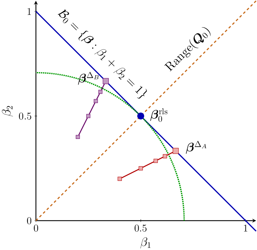


 Open access

