



1. Introduction
Since the 1960s, air traffic has grown considerably, as has noise pollution around airports. These nuisances are such that they have repercussions on human health, wildlife and house prices (Zheng, Peng & Hu Reference Zheng, Peng and Hu2020). To help reduce those issues, it is nowadays necessary to estimate the acoustic signature of an aircraft during its conception phase in order to meet acoustic certification requirements. A great deal of research has therefore turned towards identifying the main sources of noise to design devices that reduce them (see for example Li, Wang & Zhang Reference Li, Wang and Zhang2013 for a thorough review). Progress over the last 60 years has led to a tremendous reduction of the acoustic power emitted by aircrafts, by a factor 1000, almost exclusively by making changes to the propulsion system (Lockard & Lilley Reference Lockard and Lilley2004). This reduction is such that recent figures indicate that, in the approach phase,
 $50 \ \%$
of the total noise is now of airframe origin (Gittens et al. Reference Gittens, Hocquard, de Juniac, Liu and Fanning2019), i.e. caused by turbulent interactions between the air and the aircraft. As a result, a growing number of studies have focused on airframe noise, and have highlighted three major sources: slats, landing gears and flaps. For those three devices, intense noise was found to come from complex, highly unsteady flows whose analyses generally require modern experimental resources or computationally heavy simulations relying on advanced turbulence modelling.
Regarding flap noise, it was identified as one of the significant sources of airframe noise during acoustic experiments in the late 1970s and early 1980s (Kendall & Ahtye Reference Kendall and Ahtye1980)). Since then, numerous experimental and numerical studies have helped in defining a general picture of the aeroacoustic mechanisms responsible for noise production. A detailed non-exhaustive bibliography gathering both numerical and experimental works on flap side-edge noise can be found in table 1. More precisely, and as illustrated in figure 1, it was found that a dual-vortex system forms at the flap tip due to the roll-up of the flap edge shear layers. The vortex fed by the shear layer at the suction side of the flap tip is hereafter called the secondary vortex whereas the vortex fed by the shear layer at the pressure side is called the primary vortex. As the size of the primary vortex increases towards the local flap-tip thickness, the primary vortex sweeps off the suction side where it merges with the secondary vortex, resulting in a highly unsteady vortex system. For low flap deflection angle, this resulting vortex system stays near the flap surface whereas for large flap deflection angle, it further lifts off the suction side of the flap. Hence, the acoustic signature from the flap near field is closely related to the strength and size of the vortices as well as their interaction with the flap side surface. Two main mechanisms are generally described in the open literature (see Drobietz & Borchers Reference Drobietz and Borchers2006; Rossignol Reference Rossignol2010 for example), namely: (i) shear-layer unsteadiness responsible for noise at mid-to-high frequencies and radiated by the forward half of the flap and (ii) the merging vortex interacting with the sharp flap corners responsible for noise at low-to-mid frequencies and radiated by the aft half of the flap. These presumed mechanisms explain the
 $\ll \textrm {double-broadband-humps}\gg$
shape reported for flap side-edge noise spectra for various aircraft, as used in Guo (Reference Guo2011) to develop a noise prediction model and that was also confirmed in the experimental work of Bai, Lin & Li (Reference Bai, Lin and Li2022). In the latter, flap side-edge noise is shown to scale differently in the low-frequency and high-frequency domains.
Non-exhaustive summary table of numerical and experimental flap side-edge aeroacoustic studies available in the open literature. Here, AC: aerodynamic coefficients; PSD (NF/FF): near-field or far-field power spectral density; NM: noise maps; PIV: particle image velocimetry; CC: coherence/correlation coefficients; TKE: turbulence kinetic energy; circ.: vortex circulation; CML: continuous mold-line link; PRLE: protruding rounded lower-edge.

Despite recent advances that have helped to shed light on the mechanisms underlying flap side-edge noise, many grey areas remain, particularly as regards the vortex system dynamics. A striking example is the lack of knowledge of the turbulent motion length scales, which makes it impossible to define a general Strouhal number scaling linked to noise production, as pointed out by Guo et al. (Reference Guo, Joshi, Bent and Yamamoto2000). For instance, in the work of Bai et al. (Reference Bai, Lin and Li2022), the authors set an arbitrary scale of
 $1 \,\rm m$
as
 $\ll \textrm { the characteristic length scale is unknown}\gg$
. Another misunderstood feature is the possible appearance of a low-frequency quasi-tonal component in the flap side-edge spectra as reported in the work of Choudhari et al. (Reference Choudhari, Lockard, Macaraeg, Singer, Streett, Neubert, Stoker, Underbrink, Berkman and Khorrami2002) at NASA Langley, Yokokawa et al. (Reference Yokokawa, Imamura, Ura and Yamamoto2009) from JAXA, Dobrzynski et al. (Reference Dobrzynski, Nagakura, Gehlhar and Buschbaum1998) from DLR and Manoha et al. (Reference Manoha, Davy, Pott-Pollenske and Barré2018) at ONERA and DLR for instance. This quasi-tonal component is generally associated with
 $\ll \textrm {vortex instability}\gg$
but there is no physical explanation behind this tone, which makes it impossible to develop a model to predict its frequency. Yet this phenomenon is of significant interest, as underlined in the work of Dobrzynski et al. (Reference Dobrzynski, Nagakura, Gehlhar and Buschbaum1998) where they wrote: ‘How the characteristics of “tone” noise components, which were found to originate from the flap side-edge, are related to the flap side-edge vortex will be a major issue of further investigations.’ Further challenging aspects of flap side-edge flows remain: for instance a wide range of studies report the primary and secondary vortex to have a strong jet-like core, the former being the stronger. Nonetheless in some cases, the observed situation is reversed (Choudhari et al. Reference Choudhari, Lockard, Macaraeg, Singer, Streett, Neubert, Stoker, Underbrink, Berkman and Khorrami2002; Buffo et al. Reference Buffo, Wolf, Dufhaus, Hörnschemeyer and Stumpf2012) or the secondary vortex is of different nature (Farvolden et al. Reference Farvolden, Cruikshank, Okoronkwo, Baba, Ben-Gida, Lavoie, Stalnov and Moreau2024). The importance of vortex breakdown remains unclear as well. While in Drobietz & Borchers (Reference Drobietz and Borchers2006) it is assumed that vortex breakdown is not one of the main sources of noise because it does not involve solid surfaces, its appearance was linked to a complete change in flow topology in Khorrami et al. (Reference Khorrami, Singer, Radeztsky and Ronald1999).
The scope of this paper is to provide a deep analysis of the flap side-edge vortex dynamics of a well-documented configuration that precisely features a tonal component. Through advanced scale-resolving numerical simulation, a deep insight into the formation of the dual-vortex system is provided to further understand the physical mechanism behind this tonal feature. With this aim, a detailed knowledge of the spatial organisation of the pressure fluctuation field is provided ranging from the shear-layer roll-up to the merged vortex advection past the trailing edge. This paper is organised as follows: In § 1, the numerical procedure is briefly described. The test case is presented in § 2, highlighting prior experimental investigation results and providing an overview of the simulation parameters. A detailed study of the mean and unsteady flows is carried out in § 3 enabling the distinction of three different flow phases. The shear-layer roll-up (phase I) and the merging process (phase II) are analysed in § 4. The cross-flow wake developing in phase III and the advection of the merged vortex are studied in § 5. The tonal mechanism is described and discussed in § 6.
Schematic illustration of a dual-vortex system developing along a flap side edge around a realistic wing with flap deployed.

1.1. The lattice Boltzmann method
The numerical simulations in this study were carried out using the ProLB software, which is based on the lattice Boltzmann method (LBM). A discrete form of the Boltzmann equation is solved using a stream-collide algorithm
 \begin{equation} f_i\left (\boldsymbol{x} + \boldsymbol{\xi }_i \varDelta t, t + \varDelta t\right ) - f_i\left (\boldsymbol{x},t\right ) = \varOmega _i^{\textit{HRR}} + \frac {1}{2}\psi _i\left (\boldsymbol{x},t\right )\!, \end{equation}
where
 $\varDelta t$
is the time step and
 $f_i$
stands for the density distribution at position
 $\boldsymbol{x}$
and time
 $t$
of fictitious particles associated with discrete velocity
 $\boldsymbol{\xi }_i$
. The term
 $\varOmega _i^{\textit{HRR}}$
corresponds to the hybrid recursive regularized Bhatnagar Gross Krook (HRR-BGK) collision operator, which models the collision process as a relaxation of distributions
 $f_i$
towards a discrete Maxwell–Boltzmann distribution
 $f_i^{{eq}}$
happening in time
 $\tau$
. This relaxation relies on a recursive regularisation of the distributions hybridised with finite differences to significantly enhance stability, as detailed in the works of Latt & Chopard (Reference Latt and Chopard2006), Malaspinas (Reference Malaspinas2015) and Jacob, Malaspinas & Sagaut (Reference Jacob, Malaspinas and Sagaut2018). The force term
 $\psi _i$
, described in the work of Feng et al. (Reference Feng, Boivin, Jacob and Sagaut2019), is a correction term that alleviates the cubic Mach number error.
The LBM relies on the use of hierarchical isotropic Cartesian grids which, on the one hand, is very costly in the near-wall region and, on the other hand, does not conform to the boundary but instead follows a staircase pattern. To circumvent both of these issues, immersed boundary conditions based on the use of a wall model are used. The present wall treatment relies on the linearisation procedure of Tamaki, Harada & Imamura (Reference Tamaki, Harada and Imamura2017) applied to the Spalart–Allmaras (S–A) wall model of Allmaras & Johnson (Reference Allmaras and Johnson2012). This numerical procedure enhances compatibility between the grid resolution and the discrete numerical velocity gradient. The present wall treatment was proven to render smooth and accurate aerodynamic coefficients and flow prediction even for very fine near-wall grid and for various wall-bounded flows, see e.g. Husson et al. (Reference Husson, Terracol, Deck and Garrec2023).
1.2. Turbulence modelling
Due to the intrinsic unsteady nature of the LBM and its inherent dependence on wall models, it is classically associated with wall-modelled large eddy simulations (WMLES) where the outer layer of turbulent boundary layers as well as separated areas are treated in LES while the inner layer is entirely modelled. In the present case, we adopt a different strategy in order to reduce the number of grid points by a factor of approximately 30 compared with WMLES (as detailed in § 2.2) while avoiding spurious acoustic noise sources due to under-resolved turbulent structures. Thus, the turbulence model used in this study is the zonal detached eddy simulation (ZDES) mode 2 (2020). It is a multi-resolution approach developed at ONERA by Deck (Reference Deck2012) that covers a wide range of modelling from Reynolds-averaged Navier–Stokes (RANS) to wall-resolved large eddy simulation , see Deck et al. (Reference Deck, Renard, Laraufie and Weiss2014), Renard & Deck (Reference Renard and Deck2015). In this study, we are interested in the so-called mode 2 (2020) designed to treat attached boundary layers in RANS and free or separated flows in LES, contrary to WMLES approaches where the scales located in the outer region of the turbulent boundary layer also need to be explicitly resolved. The RANS/LES interface is automatically determined by the model, thanks to the dynamic computation of the length scale associated with the destruction term of the S–A model transport equation
 \begin{equation} \frac {\partial \widetilde {\nu }}{\partial t} + {\boldsymbol{u}} \boldsymbol{\cdot }\boldsymbol{\nabla } \widetilde {\nu } = c_{b1}\widetilde {\boldsymbol{\textit {S}}}\widetilde {\nu } - c_{w1} f_{w} \left (\frac {\widetilde {\nu }}{\ell _{\textit{ZDES}}}\right )^2 + \frac {1}{\sigma }\left [\boldsymbol{\nabla }\boldsymbol{\cdot }\left (\left (\nu +\widetilde {\nu }\right )\boldsymbol{\nabla } \widetilde {\nu }\right ) + c_{b2}\left (\boldsymbol{\nabla }\widetilde {\nu }\right )^2 \right ]\!, \end{equation}
where the terms
 $c_{b1}$
,
 $c_{b2}$
,
 $c_{w}$
,
 $f_{w}$
and
 $f_{v1}$
are given in the original publication by Spalart & Allmaras (Reference Spalart and Allmaras1992). The eddy viscosity
 $\nu _t$
is defined from the pseudo viscosity
 $\widetilde {\nu }$
as
 $\nu _t = \widetilde {\nu } f_{v1}$
and the hybrid length scale
 $\ell _{\textit{ZDES}}$
controls the RANS treatment of boundary layers. It is computed as
 \begin{equation} \ell _{\textit{ZDES}} = d_w - f_{P_{\textit{ZDES}}}\text{ max}\left (0,d_w - C_{{DES}} \varDelta \right )\!, \end{equation}
where
 $d_w$
is the wall distance,
 $C_{{DES}} = 0.65$
is a calibrated constant and
 $\varDelta$
is a cell-size estimate. Finally, the main parameter is the shielding function
 $f_{P_{\textit{ZDES}}}$
which ensures the RANS treatment of boundary layers based on three physical sensors
 $r_d$
,
 $G_{\widetilde {\nu }}$
and
 $G_{\varOmega }$
respectively designed to detect the log layer (to shield), the wake layer (to shield) and shear layers (to not shield). This turbulence model was validated in both the Navier–Stokes and LBM frameworks Husson, Terracol & Deck (Reference Husson, Terracol, Deck and Le Garrec2024c
) and for a wide range of flows such as a high-lift wing by Husson et al. (Reference Husson, Terracol and Deck2024a
), open rotor by Dumlupinar, Housman & Duensing (Reference Dumlupinar, Housman and Duensing2024), jet by Gand et al. (Reference Gand, Huet, Renaud and Sartor2023), space launcher by Reynaud et al. (Reference Reynaud, Weiss, Deck and Guillen2022), missile by Manueco, Weiss & Deck (Reference Manueco, Weiss and Deck2021), airfoil in stall conditions by Bouchard et al. (Reference Bouchard, Marty, Deck and Costes2022) as well as in the NASA High-Lift Common Research Model by Browne et al. (Reference Browne, Housman, Kenway, Ghate and Kiris2023). For a more thorough description of the ZDES mode 2 (2020) turbulence model, the reader is referred to the paper by Deck & Renard (Reference Deck and Renard2020).
In the present work, and complementary to the automatic mode 2 (2020) of ZDES, we further rely on a zonal approach (as in the original work of Deck Reference Deck2005) by explicitly setting fixed regions of the flow to RANS mode. This approach is very similar to the one of Housman et al. (Reference Housman, Stich, Kocheemoolayil and Kiris2019) that focuses on slat noise in high-lift wing flows within the LAVA solver developed by NASA. In their work, the main wing and the flap were manually set to RANS mode. This choice not only allows coarser mesh resolution within the RANS areas but it also suppresses any other spurious noise sources that would be radiated by LES regions (see Deck, Weiss & Renard Reference Deck, Weiss and Renard2018). In effect, the simulation is, by construction, tuned to isolate the flap side edge, which strengthens agreement near 6.6 kHz but can affect the broadband levels. Because here the emphasis is put on the flap side-edge area, the slat as well as the main element are therefore treated in RANS except within the flap cove. This zonal strategy is schematically presented in figure 2.
Schematic representation of the zonal RANS/mode 2 (2020) strategy for the present high-lift wing geometry.

2. Flap side-edge configuration
2.1. Prior wind-tunnel test investigations
The present numerical study focuses on one of the two flap side-edge configurations extensively studied during the swept airfoil with high lift (SWAHILI) experimental campaign conducted jointly by ONERA and DLR, see Manoha et al. (Reference Manoha, Davy, Pott-Pollenske and Barré2018) for a detailed description of the experiments. The aim of this campaign was twofold: assessing the influence of sweep in the acoustic emission of the wing as well as comparing noise radiated by different flap side-edge geometries. It was led in the F2 facility in Le Fauga-Mauzac, the flap side edge being mounted on a 30
 $^{\circ }$
swept wing at
 $5.3^{\circ }$
incidence. The reference stowed chord (with no-sweep angle) is equal to
 $c = 0.3 \,\rm m$
, the free-stream velocity is
 $u_0 = 71 \,\rm m\,s^{-1}$
which leads to a Reynolds number of
 ${Re}_c = 1.43 \times 10^{6}$
and a Mach number of
 ${Ma} = 0.21$
. Three configurations have been studied:
-
(i) the nominal configuration (NOM) where the flap is deployed along the full wing span with no flap side edge;
-
(ii) a flap side edge aligned with the flow direction referred to as FSA and characterised by a large gap between deployed and stowed flaps;
-
(iii) a flap side edge aligned with the sweep direction denoted FSD. The three geometries are depicted in figure 3.
Beamforming techniques have been applied to pressure signals recorded from a 120-microphone array to isolate the flap side-edge contribution to the overall noise. For each configuration, it offers a deep understanding of its frequency distribution and allows us to spatially localise acoustic sources at a given frequency. In figure 3, the integrated pressure spectra obtained for the three configurations are also plotted, showing three different behaviours.
Visual representation of the three geometries NOM, FSA and FSD studied during the SWAHILI campaign Manoha et al. (Reference Manoha, Davy, Pott-Pollenske and Barré2018) along with pressure spectra integrated in a
 $0.24 \,\rm m$
square centred at the deployed flap-tip trailing edge. The wing geometry is also represented along with the microphone array.

The NOM configuration, without the flap side edge, shows low levels of fluctuations at high frequencies and moderate levels at low frequencies. In comparison, PSD levels are much higher with the FSD configuration, from 5 dB Hz−1 at 2 kHz to 15 dB Hz−1 at 7 kHz. This illustrates the increase in noise radiation induced by the presence of a flap side edge, here in a broadband behaviour. Nonetheless, PSD levels of the FSA configuration have a broadband hump centred around 6.6 kHz (corresponding to a Strouhal number of
 ${St}_{c_{\textit{flap}}} = 8$
based on flap chord
 $c_{\textit{flap}}$
) that peaks at 60 dB Hz−1 and which is specific to this configuration. This hump is believed to be the consequence of a physical phenomenon occurring at the flap side edge for this geometry as specified in Manoha et al. (Reference Manoha, Davy, Pott-Pollenske and Barré2018), but its origin remains unknown.
Schematic representation of the 14 PIV planes for the FSA configuration. The PIV reference frame (
 $O$
, LX, LY) used for the experiments is represented and the written number corresponds to the constant value of LX or LY. Only a portion of the wing is drawn.

Figure 4. Long description
A schematic representation of the 14 PIV planes for the FSA configuration. The PIV reference frame (LX, LY) used for the experiments is represented, and the written numbers correspond to the constant values of LX or LY. Only a portion of the wing is drawn. The flow direction is indicated with arrows pointing to the right. The main wing and deployed flap are labeled. The diagram shows 8 planes where LX is constant and 6 planes where LY is constant. The values for LX range from -73 to 22, and the values for LY range from 99 to 159.
Particle image velocimetry (PIV) measurements have been performed along both slap side-edge geometries (FSA and FSD). The locations of the 14 PIV planes for the FSA configuration are shown in figure 4. The PIV datasets for both FSD and FSA configurations show very different behaviour of the vortex system, underlying the large influence of the flap geometry alone. For instance, at a same distance from the leading edge of the flap tip, the main vortex of the FSA configuration has a
 $\ll \textrm {jet-like}\gg$
core that reaches
 $1.5 u_0$
velocity whereas the one of the FSD configuration shows a velocity deficit of
 $0.5 u_0$
. As only the FSA configuration presents a quasi-tonal component, the present numerical study focuses specifically on this flap geometry in order to understand the specific features responsible for its particular noise signature. Therefore, PIV data provide a basis for validation to ensure that the various physical mechanisms involved are accurately reproduced numerically.
It is important to mention that this is not the first time that a quasi-tonal component emanating from the flap region has been reported in previous wind-tunnel studies. Indeed, previous wind-tunnel tests such as at the NASA-LTPT by Choudhari et al. (Reference Choudhari, Lockard, Macaraeg, Singer, Streett, Neubert, Stoker, Underbrink, Berkman and Khorrami2002), JAXA-LWT2 by Yokokawa et al. (Reference Yokokawa, Imamura, Ura and Yamamoto2009) and DLR-AWB by Dobrzynski et al. (Reference Dobrzynski, Nagakura, Gehlhar and Buschbaum1998) also obtained a quasi-tonal component at low frequencies radiated by the flap side edge. For the first two studies, peak frequencies were respectively
 $4.9$
and
 $1.3$
kHz but obtained for models twice as large as the current geometry. For the experiments of Dobrzynski et al. (Reference Dobrzynski, Nagakura, Gehlhar and Buschbaum1998), the authors report Strouhal numbers based on flap chord between 5 and 7 depending on the flow conditions, which are close to the one reported in this study, which is 8. Besides, let it be reminded that the lack of an adapted scaling does not allow a fair comparison between the obtained frequencies, as there is currently no model that can predict the frequency of the tone.
2.2. Simulation overview
The numerical simulation presented in this work reproduces the full wind-tunnel test section of size
 $7 \,\rm m \times 1.4 \,\rm m \times 1.8 \,\rm m$
. For cost reasons, the boundary layers that develop on the sidewalls of the test section are neglected. Therefore, these walls are instead treated using slip boundary conditions. Indeed, for a coarse Cartesian near-wall resolution of
 $\varDelta = 5.4 \times 10^{-4} \,\rm m$
(corresponding to
 $\varDelta ^{+} = \varDelta u_{\tau } / \nu \approx 100$
after one metre), the number of points associated only with the test section boundary layers would exceed one billion. Besides, accurately resolving turbulent motion within the slat and flap shear layers for the entire
 $1.6 \,\rm m$
span is also very expensive if not prohibitive. As detailed in § 1.2, it was chosen to force in RANS regions surrounding the slat and the main wing (apart from the flap cove). The slat shear layers being treated in RANS, the constraints on the grid resolution are alleviated which allows drastic cost reduction. Based on a lower-bound extrapolation of prior bidimensional simulations of the same profile (Husson et al. Reference Husson, Terracol and Deck2024a
), this zonal strategy reduces the number of grid points by a factor of 30, from approximately 4 billion to 120 million. Henceforth, the meshing effort is mainly focused on resolving the flap side-edge vortex system.
To optimise the grid-point distribution in the flap side-edge area, simulations of progressively finer resolutions have been undertaken. For a given refinement level, the mean path of the vortex system is extracted from a closed isosurface of the
 $Q$
-criterion, where
 $Q$
being the second invariant of the velocity gradient tensor, which is then injected as a volume to be meshed for the next level of refinement. As depicted in figure 5, with this strategy, the mesh is refined following the path of the primary, secondary and merged vortices instead of using a uniform box of refinement.
The LBM Cartesian grid is spread over
 $11$
levels of refinement, the finer resolution level being
 $\varDelta _{{min}} = 6.25 \times 10^{-5} \,{\rm m} = 2.1 \times 10^{-4} c$
which is only used for the main wing trailing edge and near the flap side-edge surface. It imposes a minimal time step of
 $\varDelta t _{{min}} = 1.1 \times 10^{-7} {\,\rm s} = 2.6 \times 10^{-5} c / u_0$
. The third level of refinement is used for the flap cove whereas RANS boundary layers are treated with the fourth level of resolution
 $\varDelta _{4}=5 \times 10^{-4} \,\rm m$
. This resolution was found to be a good compromise between cost and accuracy of the boundary layer prediction. The ZDES-LBM simulation was run for a total physical time of
 $t_{{tot}} = 0.18 \,{\rm s} \ (t_{{tot}} \boldsymbol{\cdot }u_{0}/c \approx 43 )$
split into
 $t_{{tr}} = 0.05{ \,\rm s} \ (t_{{tr}} \boldsymbol{\cdot }u_{0}/c \approx 12 )$
of transient phase and
 $t_{{da}} = 0.13 {\,\rm s} (t_{{da}} \boldsymbol{\cdot }u_{0}/c \approx 31 )$
of data acquisition. Absorbing layers were used at the inlet and the outlet to avoid spurious acoustic reflections.
Grid visualisation coloured by resolution level for two slices cutting through the flap side edge.

Isosurface of
 $Q-$
criterion
 $\textit {Q}^{\ast } = \textit {Q} \times {\textit {c}}^{\text{2}} / \textit {u}_{\text{0}}^{\text{2}} = \text{6000}$
coloured by velocity magnitude
 $\| {\boldsymbol {u}}\|$
. The main flow features are labelled.

Figure 6. Long description
A diagram illustrating the formation and behavior of vortices at the flap tip of an aircraft flap. Panel A: The diagram shows the formation of a dual-vortex system at the flap tip. The primary vortex is fed by the shear layer at the pressure side, while the secondary vortex is fed by the shear layer at the suction side. The diagram labels include jet-like secondary vortex, jet-like primary vortex, vortex merging, reverse flowfield, and vortex core deceleration. Panel B: The diagram shows the further development of the vortex system. The primary vortex increases in size and merges with the secondary vortex, resulting in a highly unsteady vortex system. The diagram labels include jet-like secondary vortex, flap cove hairpin vortices, jet-like primary vortex, and wake-like behavior of the shear-layer.
3. Overview of instantaneous and mean flow
3.1. Instantaneous flow
Since the formation of the dual-vortex system is strongly influenced by the Reynolds number and the flap geometry (see Francis & Katz Reference Francis and Katz1988), we begin with a general description of the formation and development of the unsteady vortical structures of the flow near the flap side edge. The idea is to draw up a clear picture of the flow topology for the current configuration. With this aim, its main features are highlighted in figure 6, which shows iso-surfaces of
 $Q$
-criterion coloured by velocity magnitude. In the present case, two
 $\ll \textrm {jet-like}\gg$
vortices form around the flap-tip edge due to the shear-layer roll-up from the pressure side (primary vortex) and from the suction side (secondary vortex). At around mid-chord of the flap, the primary vortex has grown to a size comparable to the flap side-edge thickness; it is swept over the suction side and merges with the secondary vortex to form a single highly unsteady vortical structure. Further downstream, the merged vortex lifts off the suction side of the deployed flap and is then advected away where its core undergoes a significant deceleration typical of vortex breakdown phenomenon. So far, the main characteristics of the simulated flow correspond very well to those described in the literature, see for instance Rossignol (Reference Rossignol2013). However, there are two more aspects that are rarely mentioned and particularly highlighted in figure 6. The first aspect is the interaction between the vortex system and turbulent structures advected from both the flap cove and the main wing near trailing-edge separation. Those structures are trapped by the induced velocity of the vortex system, as can be observed in the work of Casalino et al. (Reference Casalino, Fares, Duda, Hazir and Khorrami2015) and is discussed in Farvolden et al. (Reference Farvolden, Cruikshank, Okoronkwo, Baba, Ben-Gida, Lavoie, Stalnov and Moreau2024). The second aspect is the behaviour of the shear layers following vortex merging, once the vortical structure has swept over the flap suction side. They tend to act as a wake developing in the cross-flow direction. Wake is wrapped around the merged vortex and tends to slow its outer velocity.
3.2. Acoustics
In order to analyse and understand the physical mechanism responsible for the unidentified noise source around 6.6 kHz (see figure 3), it is necessary to check that it is accurately reproduced numerically. Therefore, the simulated noise radiation is compared with the processed data obtained from the experimental microphone array. The Ffowcs Williams & Hawkings acoustic analogy in its solid formulation is used to obtain the pressure fluctuation signal at each microphone of the array. It is computed with the ONERA in-house code KIM, see Rahier, Huet & Prieur (Reference Rahier, Huet and Prieur2015) and Rahier & Prieur (Reference Rahier and Prieur2025), and relies solely on the instantaneous surface pressure signal, here collected at a sampling frequency of 150 kHz. The surface pressure signal is extracted from a
 $0.4 \,\rm m$
spanwise portion of the wing centred at the flap side edge. The RANS zones (slat and a portion of the main wing) do not radiate noise, thus it is necessary to isolate the flap contribution in the experimental data to allow a fair comparison. This is done by computing noise maps using the DAMAS deconvolution process (see Brooks & Humphreys Reference Brooks and Humphreys2006) applied either to the 120 microphones of the array or the 120 corresponding observer points from the simulation. The noise map for a third-octave band frequency of 6.3 kHz is plotted in figure 7. For this frequency band, experimental data show a wide source spot centred approximately at two thirds of the flap chord. It shows that the contribution to the sudden and unexplained broadband tone comes essentially from the flap second half-chord. It is therefore highly likely that the latter is linked to the merged vortex. An important point is that this spot is recovered numerically, which shows that the simulation is able to reproduce the underlying physical mechanism. The noise radiated is nonetheless less intense by 1–2 dB and is thus less widespread. The DAMAS noise maps also offer the possibility to reconstruct noise spectra radiated from a specified region by integrating the sources within. This was achieved for the experimental data, by taking into account the flap side-edge area only in order to filter out other noise sources. The integration area consists of a central element of span
 $0.4 \,\rm m$
. This allows a fair comparison with the numerical simulation which adopts a RANS approach for the slat and the main wing. This comparison is presented in figure 8 along with a visualisation of the integration area. For frequencies over 4 kHz, there is a very good agreement between the two spectra. The typical bump obtained for the far-field spectra is recovered numerically, with a 1–2 dB Hz−1 mean difference. Further investigation for frequencies near 2 kHz has shown that a low-frequency noise source exists in the experiments near the retracted flap downstream of the flap track. This may explain the differences observed below 4 kHz as the present simulation does not contain slat and flap tracks and this area of the flow is treated with RANS in the simulation due to high CPU cost and thus does not resolve pressure fluctuations (see figure 2).
Numerical and experimental noise maps at 6.3 kHz obtained using deconvolution approach for the mapping of acoustic sources (DAMAS) process. Courtesy of Sandrine Fauqueux (ONERA, France). Here, SPL denotes the sound pressure level.

Comparison between the numerical and measured far-field pressure spectra for a given microphone. The numerical far-field spectrum is computed using an acoustic analogy from the ZDES-LBM simulation while the experimental spectrum is reconstructed by taking into account the sources emanating from the flap side-edge area only.

3.3. Mean flow
As emphasised by Guo et al. (Reference Guo, Joshi, Bent and Yamamoto2000), surface pressure fluctuation analysis is one of the key element to identify acoustic sources. It maps the trajectory of the vortex system onto the flap surface and provides an estimation of the vortex/wall interaction intensity. It can therefore be used to highlight the areas of intense fluctuations potentially responsible for the observed acoustic signature, here specific to the FSA configuration. For this reason, the root mean square (r.m.s.) of surface pressure fluctuations is plotted in figure 9.
The r.m.s. of surface pressure fluctuations
 $p'_{\textit{rms}}$
contours in dB along the flap side edge. Additional mean friction lines are plotted in black. Three phases of the flow are highlighted and for each one of them, a slice of the mean Mach numbers is shown.

Its distribution along the flap surface leads to three distinct flow phases, assumed to be governed by different characteristiic scales. Each phase, and its relation to noise generation is thoroughly described below in light of figure 9. Before going into more detail about these phases, it should be noted that distinguishing between the first two is very common in the literature, see for example the work of Drobietz & Borchers (Reference Drobietz and Borchers2006), Guo (Reference Guo2011) and Rossignol (Reference Rossignol2013).
I – The shear-layer roll-up phase. The first phase is characterised by the roll-up of the shear layers at the pressure and suction sides which is evidenced in slice 1 of figure 9. The roll-up process that forms the primary vortex is highlighted by the mean friction lines whereas the gradual widening and strengthening of the vortex can be seen following its trail along the flap edge. One can note that the shear-layer roll-up is tridimensional so that the primary vortex follows a helical path which corresponds to the observation of Guo et al. (Reference Guo, Joshi, Bent and Yamamoto2000). Both vortices show a
 $\ll \textrm {jet-like}\gg$
core. In the study of Bai et al. (Reference Bai, Lin and Li2022), it was shown that this region of the flow is primarily responsible for mid-to-high frequencies, especially due to the shear-layer unsteadiness at the sharp edges which act as efficient noise scatterers, but also as the shear layer conveys small-scale turbulent structures to impinge on the flap surface.
II – The vortex merging phase. The vortex merging is characterised by a strong interaction between the primary vortex and the secondary vortex. For the FSA configuration, the merging process starts when the primary vortex reaches a size comparable to that of the local flap thickness at
 $x/c_{\textit{flap}} = 0.5$
. It is generally assumed that the main noise source in this phase is closely linked to the interaction between the highly unsteady vortical structure and the flap surface near the flap-tip upper edge. It is known to generate noise in low-to-mid frequencies. In the present case, the highest levels of surface pressure fluctuations (exceeding 120 dB) are found in this phase at the flap upper edge.
III – The cross-flow wake phase. In the present case, a third phase characterised by a large low-speed area can be identified and is hereafter referred to as a cross-flow wake. This phase extends from a focal point (indicated in figure 9) to the flap trailing edge and can be identified from the reversed-flow area near the flap surface. Although the merged vortex has lifted off the flap suction side, there is a sudden rise in pressure fluctuation intensity which locally exceeds 120 dB. This suggests a different mechanism than vortex–structure interaction in this phase which makes it different from the previous one.
A complementary view of the mean flow organisation for each phase is presented in figure 10 where streamlines coloured by velocity magnitude are plotted following the dual-vortex system. It highlights the very strong acceleration of the vortex cores (from
 $u/u_0 = 1.6$
to
 $u/u_0 = 2.3$
for the primary vortex). It also shows that part of the vorticity that feeds the secondary vortex comes from the pressure side of the flap. Besides, it is seen that the primary vortex undergoes a significant deceleration when it sweeps over to the flap suction side whereas the secondary vortex lifts off the suction side earlier near
 $x/c_{\textit{flap}} = 0.38$
. Finally, within phase III, the merged vortex is fed by vorticity originating from the cross-flow developing on both the suction and pressure sides of the flap. The low-speed area results from the formation of a vortex that travels upstream.
Illustration of the three different phases of the dual-vortex system by velocity-magnitude-coloured streamlines along the flap side edge.

Figure 10. Long description
Illustration of the three different phases of the dual-vortex system by velocity-magnitude-coloured streamlines along the flap side edge. The image is divided into three phases: Phase 1, Phase 2, and Phase 3. Each phase shows streamlines colored by velocity magnitude, with a color scale ranging from blue (0.3) to red (1.5). Phase 1 shows streamlines with higher velocity magnitudes, predominantly in red and yellow. Phase 2 shows a transition with a mix of colors indicating varying velocity magnitudes. Phase 3 shows streamlines with lower velocity magnitudes, predominantly in blue and green.
In the following, each phase is analysed separately in the same way. The analysis is split into two steps: first, the mean field is compared with the available experimental data for validation purposes but also to complete the discussion. In the second step, the fluctuating field at the wall is analysed to identify whether this phase of the flow is responsible for the quasi-tonal component at 6.6 kHz.
Velocity norm fields
 $\|\boldsymbol{\textit {u}}\|$
obtained for the ZDES-LBM simulation (a) and the experiments (b) for the planes LX = −32 and LY = 111 (see figure 4). Two profiles are plotted, they are extracted from two rakes represented as dotted lines on the PIV contour map (c).

4. Shear-layer roll-up and vortex merging phase analysis
4.1. The shear-layer roll-up phase
During the shear-layer roll-up phase, it was observed that the ZDES-LBM simulation predicts the formation of two vortices, with the primary vortex from the pressure side being the stronger of the two. The analysis first focuses on comparing the PIV aerodynamic data available in this region of the flow. As the vortices are located very close to the wall, it is difficult to evidence their core using PIV mean velocity fields. Indeed, near-wall PIV measurements are generally blanked due to the reflection of the laser sheet onto the wind-tunnel model. Referring to figure 4 that shows the position of every PIV measurement, this region of the flow comprises the planes LX = −60, −51, −42, −32 and LY = 99, 111.
The velocity norm fields
 $\left \|\boldsymbol{\textit {u}}\right \|$
obtained with both ZDES-LBM data and PIV measurements are plotted in figure 11 for the LX = −32 and LY = 111 planes. There is a very good agreement between the simulation and the experiments, as quantitatively underlined by the two lines where flow data are extracted. The contour map of plane LX = −32 clearly shows that the primary vortex was observed during the experiments, and its size and shape are well predicted by the simulation. Both fields report a strong entrainment effect of the vortex on the stowed flap wake. For this plane, the near-wall blanking of the PIV data nonetheless prevents experimental identification of the secondary vortex. It is, however, possible to see the secondary vortex on the LY = 111 plane. Indeed, a strong vortex is clearly observed on the flap suction side which cannot correspond to the primary vortex, as shown in figure 11. Based on the simulated data for this plane, the size, position and strength of this secondary vortex are also correctly predicted. For this phase, further comparisons with other PIV measurements are not shown despite displaying the same level of agreement as they do not add further value to the discussion. This comparison shows that the mean description of the vortex system for the roll-up phase is accurately simulated. This system is effectively composed of two jet-like core vortices, which induce a significant entrainment effect. From an unsteady point of view, this phase is characterised by the coherent motion of the shear layer, as discussed below.
A PSD map of surface pressure fluctuations is presented in figure 12 for seven numbered sensors located close to the shear-layer roll-up. They are divided into three groups: probes 1 and 2 are positioned near the lower edge, probes 4 and 5 near the upper edge, while probes 3, 6 and 7 are located on the vortices paths during their formation. As expected, probes 1 and 2 are characterised by a coherent motion caused by the shedding of the shear layer at the pressure side. The frequency peak of the Kelvin–Helmholtz instability is
 $f_{{PS}} = 29.5 \text{ kHz}$
. As the primary vortex develops along the flap side edge, the shedding motion becomes more intense and more broadband due to small turbulent scales being conveyed by the roll-up process. Probes 3, 4 and 5 near the suction side edge display the same behaviour but with a lower-frequency shedding motion of
 $f_{{SS}} = 18.5 \text{ kHz}$
and without growing in intensity. Regarding probes 6 and 7 along the primary vortex path, the surface pressure spectra become broadband with higher fluctuations at high frequencies. Probe 6 is located within the helical path of the primary vortex thus displaying a hump close to 15 kHz whereas probe 7 does not.
The PSD map composed of seven surface probe points distributed over the shear-layer roll-up phase.

Figure 12. Long description
The image contains three line graphs and a 3D model of an aerodynamic structure with labeled points. Panel A: A line graph showing power spectral density (PSD) in decibels per Hertz (dB Hz^-1) versus frequency in Hertz (Hz) for point 6 and point 7. The PSD values range from 60 to 120 dB Hz^-1, and the frequency ranges from approximately 10^3 to 10^4 Hz. Panel B: A line graph showing PSD for points 3, 4, and 5 with the same axes as Panel A. The graph shows a peak around 18.5 kHz. Panel C: A line graph showing PSD for points 1 and 2 with the same axes as the previous panels. This graph shows a peak around 29.5 kHz. The 3D model in the center shows the aerodynamic structure with labeled points 1 through 7, indicating the locations where the PSD measurements were taken.
4.2. The vortex merging phase
In § 3.3, it was shown that vortex merging occurs around
 $x/c = 0.5$
. Acoustics wave emitted by the flap side edge strongly depend on the position of the merging process and it therefore seems sensible to compare the merging location with the one observed during the wind-tunnel tests. However, experimental measurements within the vortex merging phase are complex because it takes place over a short distance and very close to the flap surface. According to the position of the experimental measurements given in figure 12, the plane LX = −20 is the closest to the vortex merging process. Hence, in figure 13, the mean velocity magnitude field is plotted for both the simulated and measured fields for the LX = −20 plane. The velocity field induced by the merging vortices and their interaction with the wake of the retracted flap is very well predicted by the simulation. More specifically, extraction lines 1 cutting through the shear layer from the pressure side is in very good agreement with experimental data. However, there are two visible differences in the vortex core from the contour map. The first difference comes from the low-velocity cross-flow wake, which is more developed in the experiments. The second difference is the vortex core location; the numerical simulation predicts a vortex core located
 $6$
mm below the experimental reference for this particular PIV plane. This strongly suggests that the vortex merging process began slightly earlier during the experiments. Nonetheless, it is important to mention the variability of experimental data on the development of the mean cross-flow wake as well as the mean vortex core position.
Velocity norm fields
 $\|\boldsymbol{\textit {u}}\|$
obtained for the ZDES-LBM simulation (a) and the experiments (b) for the planes LX = −20 (see figure 4). Two profiles are plotted, they are extracted from two rakes represented as dotted lines on the PIV contour map (c).

The mean surface pressure fluctuation map investigated in § 3.3 has shown that the highest level of pressure fluctuations is reached within the vortex merging phase when the merging vortex interacts with the flap upper edge. In figure 14, pressure spectra are displayed for seven probes that belong to this phase and that can be divided into three groups. Probes 8, 9 and 10 are located near the flap pressure side edge to monitor the possible evolution of the shear layer. Probes 11 and 12 follow the path of the primary vortex at the early stages of vortex merging whereas probes 13 and 14 are positioned at the flap upper edge where the strong interaction with the vortex takes place. Probes 8, 9 and 10 display the same frequency distribution, that became more broadband compared with probe 2. Probes 11 and 12 are located along the helical path of the vortex and both exhibit a double-bump shape. The high-frequency bump is very similar between the two probes whereas the low-frequency bump for probe 11 features a peak at 1.9 kHz. The low-frequency bump is known to be associated with the primary vortex motion, as discussed in Guo et al. (Reference Guo, Joshi, Bent and Yamamoto2000) and Khorrami & Neuhart (Reference Khorrami and Neuhart2012). Probes 13 and 14 display intense levels of pressure fluctuations at low-to-mid frequencies compared to probes 11 and 12 with and high frequencies (compared) to probes 8, 9 and 10. However, none of these probes indicates that the sought noise source comes from the merging vortex phase.
The PSD map composed of seven surface probe points distributed over the merging phase.

Figure 14. Long description
The image contains three line graphs and one diagram. Panel A: A line graph showing the power spectral density (PSD) in decibels per Hertz (dB Hz^-1) against frequency in Hertz (Hz) for probe points 14 and 12. The graph highlights specific frequencies at 1.9 kHz and 15 kHz. Panel B: A line graph showing the PSD for probe points 13 and 11, with notable frequencies at 29.5 kHz. Panel C: A line graph showing the PSD for probe points 8, 9, and 10, with annotations at 10 dB Hz^-1 and -20 dB Hz^-1. The central diagram illustrates a three-dimensional object with labeled probe points and lines indicating the regions of interest corresponding to the graphs.
5. Cross-flow wake phase analysis and merged vortex advection
5.1. Development and unsteadiness of the cross-flow wake
In § 3.3, it is shown that, downstream of a focal point, a large low-speed area develops near the flap side edge and is referred to as a cross-flow wake. One of the manifestations of this phenomenon is the existence of a reversed-flow field downstream of the focal point. This is not the first time that such a flow topology has been reported for flap side-edge flows, both with numerical simulations or in wind-tunnel tests. In the work of Khorrami et al. (Reference Khorrami, Singer, Radeztsky and Ronald1999), the existence of a focal point located on the lateral edge of the flap at 2/3 chord was reported, whose appearance was linked to vortex breakdown. Since then, other experimental studies, e.g. Angland et al. (
Reference Angland, Zhang and Molin2009), Yokokawa et al. (Reference Yokokawa, Imamura, Ura and Yamamoto2009) and Farvolden et al. (Reference Farvolden, Cruikshank, Okoronkwo, Baba, Ben-Gida, Lavoie, Stalnov and Moreau2024), and numerical investigations, e.g. Angland (Reference Angland2008), have reported the existence of a focal point. In the present case, an accumulation of oil was observed during the wind-tunnel tests of Manoha et al. (Reference Manoha, Davy, Pott-Pollenske and Barré2018). This suggests that the correct flow physics is recovered numerically. This is supported in particular by the comparison between the simulated and measured velocity magnitude fields for the plane LX = −10 plane, which is shown in figure 15. The experimental velocity field clearly shows the development of the cross-flow wake which is close to that obtained numerically. The close-up view in top of figure 15 shows specifically the mean axial velocity
 $u_x$
for the cross-flow wake as well as the merged vortex. In the numerical simulation, the region of reversed flow is clearly identified with negative values of
 $u_x$
. However, the PIV data are not close enough to the wall to provide velocity information on the early stages of the cross-flow wake and thus cannot highlight the near-wall reversed-flow field. The close agreement between ZDES-LBM and PIV for the axial velocity field strongly suggests that flow reversal was also obtained during the experiments. Additionally, one can note the strong asymmetry in the velocity core due to the merging process.
Velocity norm fields
 $\|\boldsymbol{\textit {u}}\|$
obtained for the ZDES-LBM simulation (a) and the experiments (b) for the planes LX = −20 (see figure 4). Two profiles are plotted, they are extracted from two rakes represented as dotted lines on the PIV contour map (c).

To investigate the spectral content of this phase, seven surface probes within the reversed-flow phase have been extracted. They fall into two categories: probes 15, 16 and 17 are located along the edge of the flap pressure side whereas probes 18, 19, 20 and 21 follow the edge of the flap suction side. The corresponding pressure spectra are displayed in figure 16. Each probe point has a similar PSD shape characterised by a broadband peak. The closer the point is to the trailing edge, the more the peak shifts towards high frequencies, ranging from 6.6 kHz for points 15 and 18 to 11 kHz for point 21 (corresponding to Strouhal number
 ${St}_{c_{\textit{flap}}} = 8$
to
 $13$
based on flap chord
 $c_{\textit{flap}}$
). The intensity of the peak decreases as the probe gets closer to the flap trailing edge and the surface pressure fluctuation intensity is higher along the upper edge than the lower edge. Thus, the region of the flow where the intensity of pressure fluctuations is highest corresponds to the location of probes 15 and 18, where the peak is centred around a frequency of 6.6 kHz, which corresponds to the frequency obtained in the far-field spectrum. On the one hand, it therefore appears that the physical phenomenon involved persists throughout phase III. On the other hand, this phenomenon is most intense when its characteristic frequency corresponds to the frequency of the unidentified noise in the far-field spectrum. This zone thus appears to be a good candidate to generate the far-field broadband hump and is consistent with the source indicated by the noise map (see figure 7) that points towards this region.
The PSD map composed of seven surface probe points distributed over the cross-flow wake phase.

In order to check that the quasi-tonal component obtained in the far field is indeed radiated from this flow region, a near-field/far-field coherence study is carried out similar to those of Guo et al. (Reference Guo, Joshi, Bent and Yamamoto2000), Yokokawa et al. (Reference Yokokawa, Imamura, Ura and Yamamoto2009) and Kuroda et al. (Reference Kuroda, Yokokawa, Murayama, Nakahashi and Fukunishi2007). The coherence coefficient between a given far-field (FF) microphone and a surface probe (SP) is defined as
 \begin{equation} \gamma _{{\textit{FF}},{\textit{SP}}} = \frac {\left \|S_{{\textit{FF}},{\textit{SP}}}\right \|^2}{S_{{\textit{FF}}}S_{{\textit{SP}}}} ,\end{equation}
where
 $S_{{\textit{FF}},{\textit{SP}}}$
is the cross-spectral density between far-field and surface probe signals while
 $S_{{\textit{FF}}}$
and
 $S_{{\textit{SP}}}$
denote, respectively, the power spectral density of the far-field signal and the surface probe signal. The evolution of the coherence coefficient is plotted in figure 17 for probes 2, 14, 18 and 19. Beginning with probe 2, coherence levels with far-field noise are significant (near
 $0.5$
) only at a frequency of
 $f_{{PS}} = 29.5$
kHz. This frequency corresponds to the vortex shedding of the shear layer at the pressure side, as probe 2 is localised on the lower edge. This shedding motion is thus responsible for the far-field noise at this frequency. Probes 14 and 19 only display low levels of coherence with the far-field signal. Finally, probe 18 exhibits a strong coherence level (close to
 $0.6$
) at
 $6.6$
kHz. This coherence study therefore confirms that the mechanism generating the tonal noise is generated locally near probe 18. Further investigations on the origin of this mechanism are detailed in § 6.
Coherence coefficients between the far-field microphone and near-field probes 2, 14, 18 and 19 (respectively in red, green, blue and black). Each probe localisation is reported in the top sketch. The reference far-field signal is represented in light grey and exhibits two humps at 6.6 and 29.5 kHz.

Velocity norm fields
 $\|\boldsymbol{\textit {u}}\|$
obtained for the ZDES-LBM simulation (a) and the experiments (b) for the planes LX = 22 (see figure 4). Profiles of axial and radial velocity as well as the vortex circulation are plotted (c) for a same profile as a function of the distance to the vortex core centre
 $r$
. The viscous radius
 $r_c$
refers to the distance where the value of
 $u_{\theta }$
is maximum. The dashed lines represent the theoretical profile given by a Burgers vortex.

5.2. Advection of the merged vortex
Once the merged vortex has passed the trailing edge of the flap, it is advected into the free field. The highly unsteady vortex strongly interacts with the wake developing at the deployed flap trailing edge but also at the retracted flap trailing edge, as detailed in the work of Farvolden et al. (Reference Farvolden, Cruikshank, Okoronkwo, Baba, Ben-Gida, Lavoie, Stalnov and Moreau2024). Based on the measured PIV data, the authors mention that this entrainment effect caused by the merged vortex could be responsible for far-field noise. In the present case, the experimental data allow for a more accurate quantification of the merged vortex, as it is no longer close to the wall. A comparison of the velocity magnitude field is shown in figure 18 for plane LX = 22. Both datasets show a remarkable agreement, especially for the interaction of the merged vortex with the surrounding wakes. The deployed flap wake corresponds to the large low-velocity area at the bottom left of the vortex core whereas the stowed flap wake is located at the top right. Surprisingly, there is a third low-velocity zone to the right of the vortex, found in both the experimental data and the numerical simulation. This area corresponds to the cross-flow wake wrapping around the merged vortex. There is an excellent agreement between simulations and experiments, except within the very core of the merged vortex where the velocity is overestimated by approximately
 $15 \ \%$
in the simulation. The origin of this difference remains unclear but it is supposedly linked to the slat and main wing being forced in RANS mode, which prevents the prediction of the correct deceleration due to the mixing between the vortex and the turbulent structures coming from the suction side of the main wing. It is the mean turbulent kinetic energy (TKE) level
 $k = 0.5 (u^{\prime 2}_{\textit{rms}} + v^{\prime 2}_{\textit{rms}} + w^{\prime 2}_{\textit{rms}} )$
that suggests this hypothesis. Indeed, TKE levels within the wakes are underestimated in the simulation whereas they are overestimated within the core of the vortex. Another possibility is the slight discrepancy in the location of the vortex merging that occurs slightly upstream in the experiments. The earlier development of the cross-flow wake could slow down the vortex core, as seen in § 4. It is worth noting that the laser doppler velocimetry measurements, which were only carried out for the FSD configuration, reported lower axial velocities than the PIV measurements, with differences of up to 10–15
 $\rm m\,s^{-1}$
that could also explain this difference. As the cross-flow wake development is governed by the entrainment effect of the merged vortex whose effects are greatly predicted by the simulation, the discrepancies in axial velocity should not have significant influence on the present acoustic mechanism. Nonetheless, the vortex core centre location is well predicted and is less than a millimetre away from the one measured during the experiments.
To quantify the development of the merged vortex, the axial velocity
 $u_x$
, radial velocity
 $u_{\theta }$
, circulation
 $\varGamma = 2 \pi r u_{\theta }$
and helix angle
 $\gamma = \text{arctan} [u_{\theta }/u_x ]$
are also plotted in figure 18 as a function of the distance
 $r$
from the vortex core centre. The plots are compared with theoretical plots of a Burgers vortex for radial velocity and circulation. Its radial velocity profile is given by the general formula
 \begin{equation} u_{\theta }\left (r\right ) = \frac {\varGamma _0}{r}\left (1 - e^{-1.256(r/r_c)^2}\right )\!, \end{equation}
where
 $\varGamma _0 = 0.834\, \rm m^2\,s^{-1}$
is a reference circulation that has been computed from the radial velocity profile. According to Delery (Reference Delery1994), this formula is a good representation of most vortices. In the present case, the radial velocity profiles obtained from simulation and experiments follow this theoretical behaviour although the axial velocity profile is greatly influenced by the wakes. Consequently, the circulation profiles are in good agreement within approximately two viscous radii. The helix angle profile, which is a theoretical indicator of vortex breakdown, is in good agreement with the experimental measurements. Despite having an unconventional shape due to the wake continuously feeding vorticity, the helix angle value is around 50
 $^{\circ }$
, which is a theoretical value that indicates the onset of vortex breakdown as stated by Delery (Reference Delery1994). This aspect is explored in more detail in § 6.3.
6. Acoustic mechanism underlying the tonal component in the flap side-edge spectra
Spectra for probe points 16, 18, 19, 20 and 21 against frequency or Strouhal number
 ${St}_{e} = fe/u_0$
based on the local flap thickness
 $e$
. Three instantaneous snapshots of velocity magnitude are displayed for sensors 18, 19 and 20 to highlight the development of the cross-flow wake.

6.1. Description of the proposed mechanism
In the previous section, the 6.6 kHz broadband hump in the flap side-edge spectra is shown to emanate from downstream of a focal point, where the flow is characterised by the development of a cross-flow wake. Each surface pressure probe within this region exhibits a broadband hump with a main frequency ranging from 6.6 to 11 kHz depending on its distance to the flap trailing edge. From those two elements, the spectral hump is assumed to relate to blunt trailing-edge noise. Unlike sharp trailing-edge noise which is broadband due to boundary layer turbulence scattering at the trailing edge, blunt trailing-edge noise is generally associated with vortex shedding whose shedding frequency scales with velocity
 $u_0$
and trailing-edge thickness
 $e$
such that
 \begin{equation} {St}_{e} = \frac {\textit{fe}}{u_0} \approx 0.21 ,\end{equation}
as shown in various studies (see for example Brinich, Boldman & Goldstein Reference Brinich, Boldman and Goldstein1975; Manoha, Troff & Sagaut Reference Manoha, Troff and Sagaut2000; Bae & Moon Reference Bae, Jeong and Moon2009; Collison, Stimpson & Desvard Reference Collison, Stimpson and Desvard2015 and Ali, Azarpeyvand & Da Silva Reference Ali, Azarpeyvand and Da Silva2018). The distinctive feature here is that it is the side of the flap that acts as a trailing edge, and not the flap trailing edge itself. The spectral hump is thus assumed to scale with the local flap thickness. This is due to the fact that the flow direction is deflected in the transverse direction by the merged vortex entrainment effect. To verify whether the blunt side trailing-edge assumption is valid, surface pressure spectra for probes 16, 18, 19, 20 and 21 are plotted against local-flap-thickness-based Strouhal number
 ${St}_{e}$
in figure 19. All spectra collapse to
 ${St}_{e}\approx 0.2$
, which corroborates the aforementioned hypothesis. Additional instantaneous visualisations of the cross-flow wake are also plotted in figure 19 for 3 slices passing through probes 18, 19 and 20. These snapshots highlight the increase in the wake shedding frequency combined with the decrease of the local flap thickness.
The periodic nature of the cross-flow wake motion is investigated through phase averaging in figure 20. For five probes located along the cross-flow wake at two spanwise locations, the pressure signals are phase averaged and plotted in a non-dimensional form to allow comparison. Each phase averaging is split into 50 phases. These probes were chosen because probes 18 and 22 show strong coherence at
 $x/c_{\textit{flap}} \approx 0.8$
(where
 ${St}_{e} \approx 0.21$
corresponds to
 $f \approx 6.6$
kHz) whereas pressure signals of probes 19, 23 and 24 show strong coherence at
 $x/c_{\textit{flap}} \approx 0.95$
(where
 ${St}_{e} \approx 0.21$
corresponds to
 $f \approx 10.5$
kHz); see figure 19 where pressure spectra of probes 18 and 19 are plotted. For the five signals, the phase-averaged pressure signals exhibit a wave pattern, underlining that the shedding of the cross-flow shear layers along the cross-flow direction is strongly periodic. More precisely, the phase-averaged signals from probes 18, 19 and 23 that are located very close to the flap edge result in a almost sinusoidal shape, hence are almost perfectly periodic. The wave pattern is still obtained for probes 22 and 24 but noticeable hydrodynamic contributions are evidenced for phase numbers between 20 and 40. Indeed, the two probes are located farther in the cross-flow wake development where the cross-flow wake interacts with the induced velocity of the unsteady merged vortex as well as turbulent structures originating from the wake of the main wing, as seen in the two snapshots of figure 20. This hydrodynamic interaction is the strongest near
 $x/c_{\textit{flap}} \approx 0.8$
at probe 22 because the vortex is still merging and is located very close to the flap suction side. As a result, the mean cross-flow velocity at the suction side is close to
 $\sqrt {v^2+w^2} \approx u_{0}$
whereas near the flap trailing edge it approaches
 $\sqrt {v^2+w^2} \approx 0.75 u_{0}$
. As the intensity of the pressure fluctuations scales both with the local velocity (higher-velocity fluctuation amplitude in the wake) and trailing-edge thickness
 $e$
(larger surface for scattering), and both quantity decreases along the flap edge, this explains why the resulting far-field acoustic spectrum peaks at
 $6.6$
kHz where the phenomenon is the more intense. For example, the pressure fluctuation amplitude at probe 18 (
 ${St}_{e}$
corresponding to 6.6 kHz) is 5.5 time higher than the one at probe 19 (
 ${St}_{e}$
corresponding to 10.5 kHz).
(a) Instantaneous
 $Q$
-criterion and volume slices along the cross-flow direction coloured by cross-flow magnitude
 $\sqrt {v^2+w^2}/u_0$
. (b) Phase-averaged signals for the five probes 18, 19, 22, 23 and 24. Their locations are indicated in the instantaneous snapshots. The notations
 $\overline {p}_{\varphi }$
and
 $\overline {p}$
refer, respectively, to the phase-averaged and temporal mean of the pressure signal whereas
 $p_0=101325$
Pa is the reference pressure.

Figure 20. Long description
Panel A: Two visualizations show shedding motion from a shear layer. The color scale ranges from blue to red, indicating different magnitudes. Probes 18 and 22 are marked on the left visualization, while probes 19, 23, and 24 are marked on the right visualization. Panel B: Two line graphs display phase-averaged signals for the probes. The left graph shows signals for probes 18 and 22, with the x-axis labeled Phase number and the y-axis labeled (p_phi - p_bar)/p_0. The right graph shows signals for probes 19, 23, and 24, with the same axis labels. The signals exhibit different trends and patterns for each probe.
It appears that the mechanism generating the quasi-tonal component of flap side-edge noise in the present case is the result of side trailing-edge noise. Indeed, the entrainment effect of the merged vortex is such that the flow is strongly deflected in the transverse direction, and therefore
 $\ll \textrm {sees}\gg$
the side of the flap as a trailing edge. Its location is governed by the development of the primary vortex and thus depends on the Reynolds number. This is consistent with the results of Dobrzynski et al. (Reference Dobrzynski, Nagakura, Gehlhar and Buschbaum1998) who found the tonal frequency to shift towards higher frequencies for increasing free-stream velocity. This mechanism is schematically illustrated in figure 21 for a slice along the cross-flow direction. This phenomenon occurs across the entire flap side edge from the focal point to the flap trailing edge. It is most intense at the focal point and least intense at the trailing edge, explaining why the peak exhibits a broadband nature at the far-field microphone. Thus, the peak frequency can easily be estimated from the local flap thickness near the focal point. Besides, this mechanism manifests itself in the form of an area of reverse flow near the wall and the existence of a focal point. Those two elements can be spotted with skin friction lines in numerical simulations or oil visualisations in wind-tunnel experiments.
Additionally, side trailing-edge noise could be mitigated with existing noise reduction devices such as a porous side edge to weaken the primary vortex Angland et al. (Reference Angland, Zhang and Molin2009) or flap fences to prevent the primary vortex sweeping over the suction side Guo & Joshi (Reference Guo and Joshi2003). Besides, trailing-edge noise is often mitigated based on serrations or brushes that could be adapted to the side edge, see Li et al. (Reference Li, Wang and Zhang2013).
Schematic illustration of the flow phenomena occuring within the cross-flow wake phase and its link to noise generation. The illustration represents a view from a slice along the cross-flow direction.

6.2. Generalisation to other configurations and main parameters of influence
The present acoustic mechanism, namely the side trailing-edge noise, has been observed and related to far-field noise spectra only for this configuration. This raises questions about the generalisation of this phenomenon to other flap configurations or Reynolds numbers.
Regarding flap configurations, and to the authors’ knowledge, three previous wind-tunnel tests for different flap models have exhibited an unexplained tonal component: the first one was reported in the experimental work of Dobrzynski et al. (Reference Dobrzynski, Nagakura, Gehlhar and Buschbaum1998), the second one during the wind-tunnel test campaign reported in Choudhari et al. (Reference Choudhari, Lockard, Macaraeg, Singer, Streett, Neubert, Stoker, Underbrink, Berkman and Khorrami2002) and the third one in the study of Yokokawa et al. (Reference Yokokawa, Imamura, Ura and Yamamoto2009). In the latter, a focal point as well as a region of reversed flow is observed with oil visualisations, as shown in figure 22. Thus, this strongly suggests the presence of side trailing-edge noise. In their work, the authors report a
 $\ll \textrm {low-frequency tonal noise component around 1.3 kHz}\gg$
for a configuration where the flap chord is
 $0.18 \,\rm m$
and a free-stream velocity of
 $50 \,\rm m\,s^{-1}$
. According to the visualisation, the cross-flow wake starts to develop near
 $x/c=0.75$
with a local flap side-edge thickness of
 $0.008 \,\rm m$
for this station. This leads to a Strouhal number of
 ${St}_{e} = 1300 \boldsymbol{\cdot }0.008 / 50 = 0.208$
which corresponds very well with blunt side trailing-edge noise. Besides, this tonal feature radiated by the flap side edge is obtained for multiple angles of attack and for the four tested flap geometries as well. Similarly, the tonal feature observed for flap side-edge noise in the experimental work of Dobrzynski et al. (Reference Dobrzynski, Nagakura, Gehlhar and Buschbaum1998) persists for the five angles of attack tested.
Similar flow topology experimentally observed with oil on the OTOMO model from JAXA. For this model, the flap chord is
 $0.18 \,\rm m$
and free-stream velocity is
 $50 \,\rm m\,s^{-1}$
. Adapted from the work of Yokokawa et al. (Reference Yokokawa, Imamura, Ura and Yamamoto2009). Courtesy of Y. Yokokawa, T. Imamura, H. Ura and K. Yamamoto, from JAXA, Japan.

In the SWAHILI experiment, two flap geometries were tested with all other parameters being equal. Only the FSA configuration exhibited a tonal component whereas the acoustic spectra for the FSD configuration remained fully broadband (see figure 3). To better understand why, a numerical simulation of the FSD configuration was performed on a similar but coarser grid in the flap side-edge region. The coarser mesh contains
 $76$
million nodes with
 $\varDelta x_{{min}} = 2.5 \times 10^{-4} \,\rm m$
and
 $\varDelta t_{{min}} = 4.2 \times 10^{-7} \,\rm s$
which is four time coarser than for the mesh of the FSA configuration. For the sake of clarity, details of the flow for the FSD configuration are available in Appendix A of the article. There are notable differences in the formation of the vortex system between the two configurations. First, only a single vortex develops with the FSD configuration, whereas two vortices are formed with the FSA configuration. Second, the vortex paths are also very different due to the misalignment between the flap side edge and the free-stream flow direction for the FSD configuration. Indeed, they are represented and compared in figure 23 for both numerical and experimental data (when the core of the vortex can be identified). There is a good agreement between the two datasets that both show that, in the case of the FSD configuration, the vortex no longer interacts with the flap edge in the last third of the chord, which corresponds to the location of the tonal noise source for the FSA configuration. This comparison shows the sensitivity of the vortex system development regarding flap geometry, especially the rake angle. This is because side trailing-edge noise occurs whenever the vortex system is located above the suction side and near the flap edge, and it is most intense when it is closest to the suction side. This suggests that the present mechanism is morel likely to occur for flap side edge aligned with the flow or slightly raked into the flow.
Schematic representation of the FSA (a) and FSD (b) flap side-edge geometries along with experimental and numerical vortex paths. The PIV planes are represented in dotted lines and arrows indicate the flow direction.

Regarding the influence of the Reynolds number, the appearance of side trailing-edge noise is closely related to the development of the dual-vortex system. Therefore, previous studies may provide insights into the possible persistence of this mechanism at very high Reynolds numbers. Indeed, to the authors’ knowledge, all studies that report a tonal component in flap side-edge spectra exhibit a Reynolds number based on wing chord between 1 and 2 million. In general, an increase in the Reynolds number is accompanied by a decrease in the size of the vortices and a change in the vortex path along the tip (see Francis & Katz Reference Francis and Katz1988 for instance) but the general physics of the flow stays the same. Some studies also seem to indicate a low dependence of the vortex system formation on the Reynolds number, in the sense that the physics involved remains the same. In the work of Berkman et al. (Reference Berkman, Khorrami, Choudhari and Sadowski2000) for instance, it is mentioned that the dominant features of the flap side-edge flow are relatively independent of the Reynolds number for
 ${Re}_c \gt 7 \times 10^6$
(experiments were carried out as far as
 ${Re}_c = 19.2 \times 10^6$
). Nevertheless, the authors report the appearance of vortex breakdown, as for other studies such as Khorrami et al. (Reference Khorrami, Singer, Radeztsky and Ronald1999) or Farvolden et al. (Reference Farvolden, Cruikshank, Okoronkwo, Baba, Ben-Gida, Lavoie, Stalnov and Moreau2024).
More generally, side trailing-edge noise should appear as long as the merged vortex stays in the vicinity of the flap suction side, as observed in all cases where such a tonal feature was reported. As a result, the main parameters of influence are the same as those governing the location and development of the vortex system, namely the flap deflection angle
 $\delta _{F}$
, the Reynolds number
 ${Re}_c$
and the flap geometry. Indeed, the appearance of side trailing-edge noise is heavily governed by phase I especially with the location of vortex merging (indirectly influencing the local flap edge thickness
 $e$
) and the velocity magnitude of the cross-flow
 $u_0$
. Nonetheless, the main physical phenomenon that could arise and alter the present mechanism is vortex breakdown.
6.3. Possible link with vortex breakdown of the merged vortex in the present case
Vortex breakdown is a flow phenomenon characterised by a sudden and brutal change in the vortex structure that generally occurs when the vortex radial velocity
 $u_{\theta }$
is too strong compare with its axial velocity
 $u_x$
. This change can take several forms such as a bubble that can be visualised in a hydrodynamic tunnel, e.g. Werlé (Reference Werlé1954). Vortex breakdown can be associated with areas of flow reversal, and has been linked to the appearance of a focal point for flap side-edge flows, as in the study of Khorrami et al. (Reference Khorrami, Singer, Radeztsky and Ronald1999). The Rossby number
 ${\textit{Ro}}$
is one of the most commonly used criteria for estimating the onset of vortex breakdown (for instance in Spall, Gatski & Grosch Reference Spall, Gatski and Grosch1986; Delery Reference Delery1994). It is defined as the ratio between inertial and rotational momentum
 \begin{equation} {\textit{Ro}} = \frac {r_c u_x\left (0\right )}{\varGamma _0}. \end{equation}
According to Robinson, Barnett & Agrawal (Reference Robinson, Barnett and Agrawal1994), a vortex is stable if
 ${\textit{Ro}} \geqslant 1.4$
, is unstable if
 $0.9 \leqslant {\textit{Ro}} \leqslant 1.4$
and breakdown appears if
 ${\textit{Ro}} \leqslant 0.9$
. This is in agreement with the findings of Spall et al. (Reference Spall, Gatski and Grosch1986) for leading-edge-type vortices. Although estimating the onset of vortex breakdown from a single numerical criterion is an oversimplification of reality, it has provided consistent results for delta wing vortices (Riou, Garnier & Basdevant Reference Riou, Garnier and Basdevant2010) which possess very similar properties to the vortex considered here.
Evolution of the Rossby number Ro for several planes along the flap side edge.

The vortex merging phase leads to a strong asymmetry of the vortex. Besides, although the matched vortex has a radial profile in the LX = 22 plane close to that of a Burgers vortex, it is not yet completely symmetrical. As a result, as proposed in Ben-Gida et al. (Reference Ben-Gida, Baba, Stalnov, Moreau and Lavoie2024), the vortex circulation is computed as follows:
 \begin{equation} \varGamma _0 = \int _{S_{v}} \left \|\boldsymbol{\varOmega }\right \| \text{d}S_{v}, \end{equation}
where
 $S_{v}$
denotes the vortex surface identified by the
 $\lambda _2$
criterion and
 $\left \|\boldsymbol{\varOmega }\right \|$
is the local vorticity magnitude. The
 $\lambda _2$
criterion is obtained by computing the three eigenvalues
 $\lambda _1 \geqslant \lambda _2 \geqslant \lambda _3$
of the tensor
 $\boldsymbol{S}^2 + \boldsymbol{\varOmega }^2$
, where
 $\boldsymbol{S}$
and
 $\boldsymbol{\varOmega }$
respectively correspond to the strain-rate and rotation-rate tensors. For a given section across the vortex, the surface
 $S_{v}$
corresponds to the set of points where two eigenvalues are negative, which is equivalent to
 $\lambda _2\leq 0$
. Then, the effective radius is obtained as
 $r_c = \sqrt {S_v / \pi }$
. The surface
 $S_{v}$
more accurately represents the shape of the merging vortex. In figure 24, the computed Rossby number is plotted at several stations along the vortices path. Before vortex merging, only the primary vortex value is displayed. According to the criterion of Robinson et al. (Reference Robinson, Barnett and Agrawal1994), the primary vortex is on the verge of instability and the vortex merging seems to stabilise the merging vortex. A possible explanation is the rapid growth of the effective radius while maintaining a very high axial velocity. The vortex then becomes unstable at a distance close to
 $0.7$
of a flap chord from the flap trailing edge and breaks down downstream at
 $0.9$
of a flap chord. This distance corresponds to the sudden drop in axial velocity and comes with a slight increase in kinetic energy, which is also observed in Deck & Luckring (Reference Deck and Luckring2016). The vortex breakdown thus happens at approximately one flap chord distance from the flap trailing edge. This distance seems high to explain the influence of vortex breakdown on the vortex system in the present case, contrary to the observation of Khorrami et al. (Reference Khorrami, Singer, Radeztsky and Ronald1999).
7. Conclusion
In this paper, the possible appearance of a tonal component in flap side-edge spectra is investigated. With this aim, a swept high-lift wing known to feature such a tonal component is thoroughly analysed numerically with a combination of ZDES and LBM. The simulation is able to reproduce numerically the tonal noise radiated by the flap side edge. The mean flow as well as the fluctuating field is characterised and systematically compared with experimental data. The so-called dual-vortex system typical of blunt flap side-edge flows is obtained as well with the present configuration. It is found that the near-field flow can be decomposed into three phases: phase I is characterised by the rapid roll-up of the shear layers at the pressure (primary vortex) and suction (secondary vortex) sides, phase II corresponds to vortex merging where the primary vortex is swept over the suction side and begins to merge with the secondary vortex whereas phase III corresponds to a sudden development of a cross-flow wake driven by the merged vortex.
Although phases I and II are commonly described in the literature and correspond to classic features associated with most flap side-edge vortex dynamics cases (see Rossignol Reference Rossignol2013 or Drobietz & Borchers Reference Drobietz and Borchers2006 among others), the latest phase is, however, not addressed in the open literature. In order to characterise the fluctuating pressure field, each phase was scrutinised and compared with the available experimental data. Phase I shows high-frequency peaks corresponding to the shear-layer roll-up signature (29.5 kHz at the flap side-edge pressure side and 18.5 kHz at its suction side), whereas the spectral content of phase II is dominated by low-to-mid-frequency levels of pressure fluctuations that account for the large-scale motion interacting with the upper edge of the flap. Based on a coherence analysis, it is shown that the unidentified noise source is radiated from phase III. In this phase, pressure spectra are characterised by a large bump for which the main frequency has been shown to depend on the local flap side-edge thickness
 $e$
such that the resulting Strouhal number is
 ${St}_{e} \approx 0.21$
. This phenomenon can be attributed to blunt trailing-edge noise caused by the cross-flow. The sudden change in direction causes the flow to
 $\ll \textrm {see}\gg$
the flap side edge as a trailing edge and is responsible for the noise radiated near 6.6 kHz for this configuration. The mean of the phase-averaged pressure signals in the cross-flow wake has highlighted its periodic shedding throughout the last third of the flap chord. Further discussion on this acoustic mechanism based on the open literature suggests that the present mechanism is consistent with previous experimental campaigns on different flap geometries led by NASA in Choudhari et al. (Reference Choudhari, Lockard, Macaraeg, Singer, Streett, Neubert, Stoker, Underbrink, Berkman and Khorrami2002), JAXA in Yokokawa et al. (Reference Yokokawa, Imamura, Ura and Yamamoto2009) and DLR in Dobrzynski et al. (Reference Dobrzynski, Nagakura, Gehlhar and Buschbaum1998). A brief comparison with the FSD configuration has shown that the present tonal source is more likely to happen for flap side edges aligned with a flow or slightly raked into it. Regarding the influence of the Reynolds number, the present mechanism has been observed for Reynolds numbers based on a wing chord ranging from
 $1$
to
 $2$
million. The possibility that vortex breakdown occurs earlier at higher Reynolds number may alter the present mechanism and could be the subject of further studies.
Funding
This work was supported by the Direction Générale de l’Aviation Civile (DGAC) in the frame of the BALBUZARD project under grant agreement 2021–27. The authors are grateful to S. Fauqueux and E. Manoha from ONERA for their support in acoustic post-processing and for providing the experimental data.
Declaration of interests
The authors report no conflict of interest.
Appendix A. Brief analysis of the FSD configuration
In this section, a brief description of the flow topology obtained numerically for the FSD configuration on a coarse mesh is presented. The idea is to compare the two configurations to understand why side blunt trailing-edge noise occurs with the FSA configuration but does not with the FSD configuration.
An overview of the main flow features is shown in figure 25 where iso-surfaces of
 $Q$
-criterion coloured by velocity magnitude are plotted. It shows that a strong vortex develops from the shear-layer roll-up at the flap pressure side. The vortex develops until it reaches the flap suction side where it is pushed away from the flap edge and suddenly breaks down going from a jet-like core with velocity up to
 $2 u_0$
to a core with velocity deficit down to
 $0.5 u_0$
. As the gap between the retracted and deployed flap is very small, turbulent structures from the flap cove are convected by the vortex.
Iso-surfaces of Q-Criterion
 $Q^{\ast } = Q \times c^2/u_0^2 = 3000$
coloured by velocity magnitude
 $\|\boldsymbol{u}\|$
for the FSD configuration. The main flow features are labelled.

This drastic change in flow topology results in significant differences in wall pressure fluctuation intensity, as represented in figure 26 where the r.m.s. values of pressure fluctuations are compared. A first point to note is that the small gap between the flaps induces a separation near the leading edge. A second difference comes from the shear-layer roll-up which is thicker in the FSD configuration than in the FSA configuration due to the angle between the upstream flow direction and the flap edge raked away from the flow that directly alters the vortex roll-up. In the last third chord, the FSD configuration shows very low level of pressure fluctuation intensity compared with FSA.
Comparison of r.m.s. of surface pressure fluctuations between the FSA and FSD flap configurations.

The flow field at plane LX = 22 between ZDES-LBM and PIV is plotted in figure 27 (same plane as in figure 18 for comparison with the FSA flow field). This comparison shows a good quantitative agreement between simulation and experiments. The noticeable differences are that the vortex core is slightly thicker in the simulation and its core is located
 $7.5$
mm closer to the left. Nonetheless, both datasets shows a vortex core with a velocity deficit that is rolled-up between the deployed flap wake (left) and the retracted flap wake (right). This fair agreement between the ZDES-LBM computation and PIV dataset shows that the main features of the flow physics are well reproduced by the simulation.
Comparison of velocity magnitude field between ZDES-LBM and PIV for the plane LX = 22 for the FSD configuration.


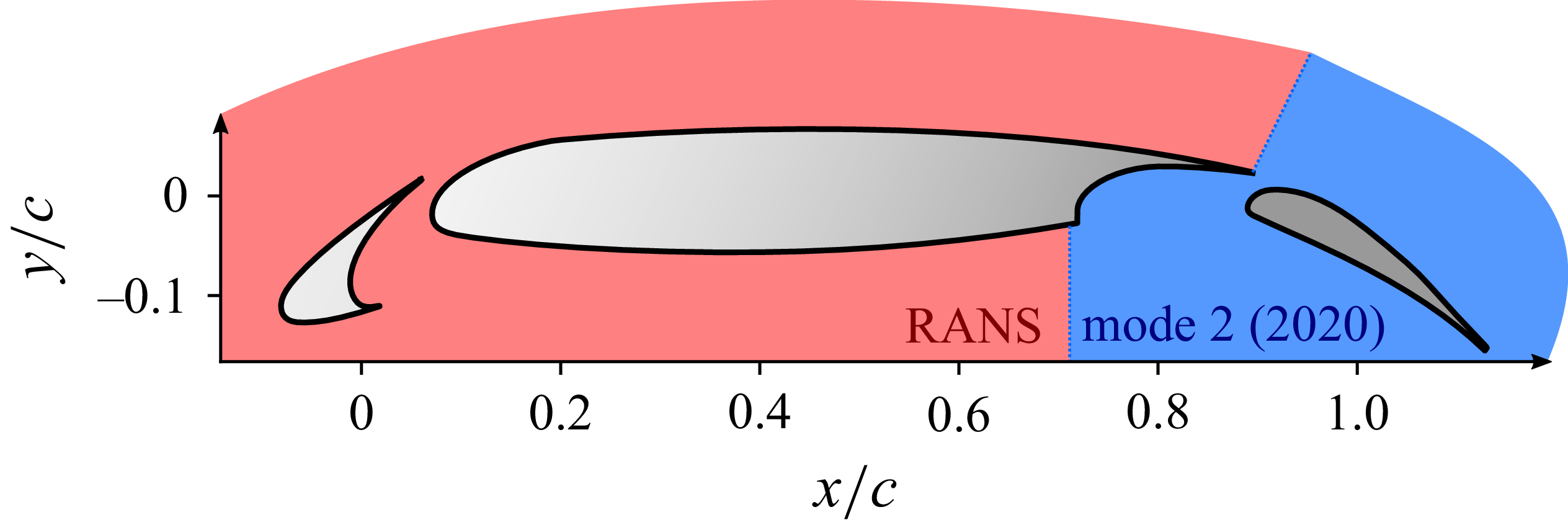

 0.24m

 O


 Q−
 Q∗=Q×c2/u02=6000
 ‖u‖


 prms′


 ‖u‖


 ‖u‖


 ‖u‖


 ‖u‖
 r
 rc
 uθ

 Ste=fe/u0
 e

 Q
 v2+w2/u0
 p¯φ
 p¯
 p0=101325


 0.18m
 50ms−1


 Q∗=Q×c2/u02=3000
 ‖u‖



