Nomenclature
- AI
-
Artificial Intelligence
- ML
-
Machine Learning
- DMD
-
Dynamic Mode Decomposition
- MTOW
-
Maximum TakeOff Weight
- MISO
-
Multi-Input Single-Output
- SISO
-
Single-Input Single-Output
- TRQ
-
Engine Torque
- WF
-
Fuel Flow
- COL
-
Collective Pitch
-
 $T_1$
-
Intake air temperature
-
$T_{oil}$
-
Oil temperature
-
$P_{oil}$
-
Oil pressure
-
$P_0$
-
Intake pressure
- NR
-
Main rotor speed
- TAT
-
True air temperature
- NP
-
Power turbine speed
- NG
-
Gas turbine speed
- NGR
-
Corrected gas turbine speed
- AIRSPEED
-
Air speed
- FFNN
-
Feed-Forward Neural Network
- RNN
-
Recurrent Neural Network
- LSTM
-
Long Short-Term Memory
- MSE
-
Mean Squared Error
- MAE
-
Mean Absolute Error
- rMAE
-
Relative Mean Absolute Error
- SINDy
-
Sparse Identification of Nonlinear Dynamics
- SINDyc
-
SINDy with control
- PySINDy
-
Python library for Sparse Identification of Nonlinear Dynamics
-
$D_{train}$
-
Training dataset (162 flights)
-
$D_{val}$
-
Validation dataset (18 flights)
-
$D_{test}$
-
Test dataset (16 flights with high-frequency sweep maneuvers)


1.0 Introduction
Real-time control of helicopter turboshaft engines has always been a complex challenge due to the stringent requirements of robust engine models capable of accounting for the strong coupling between the engine and the helicopter drivetrain. In fact, the effective implementation of control systems has always been recognised as essential for enhancing helicopter performance, monitoring and handling, as well as minimising fuel supply oscillations and rotor speed fluctuations [Reference Corliss1, Reference Mihaloew, Ballin and Ruttledge2]. High-fidelity aero-thermodynamic simulations, while invaluable for detailed analysis, are often unfeasible for real-time applications due to their computational complexity and iterative nature, significantly increasing execution time. Simplified aero-thermodynamic models based on reduced-order modeling approach have been proposed as possible alternatives to allow for the real-time applications, still exhibiting many differences in results compared to full transient high-fidelity simulations [Reference Fuksman and Sirica3]. Although often built upon static maps and linear approximations with corrections to account for environmental conditions [Reference Volponi4], these physics-based models, dating back to the 1980s [Reference Ballin5], are grounded in thermodynamic principles and rely on a detailed physical description of engine components that enhances their robustness and reliability. Recent studies (see e.g. [Reference Yazar6–Reference Mao8]) have focused on simulating engine behaviour for control applications. As mentioned above, the execution of real-time simulation of physically driven models is challenging, and many compromises are therefore necessary to develop engine models that can easily be exploited for system control, fault detection and diagnostics. By sacrificing some aspects of the engine’s physical representation, two of the most straightforward approaches involve simplified real-time engine simulations based on piecewise linear state-space perturbation models or transfer function models. These methods enable coverage of the entire operating range while supporting operational requirements [Reference Duyar, Gu and Litt9–Reference Castiglione13]. Both rely on tabulated steady-state engine performance at key operating points, with engine dynamics evaluated either through partial derivative approximations around these points (state-space perturbation) or via transfer functions such as lead-lag compensators. Although these models are less accurate than full transient high-fidelity simulations, they strike a practical balance between computational efficiency and fidelity, making them widely applicable in real-world operational scenarios. Still, developing and fine-tuning these models requires a significant effort, as they rely on extensive and costly flight campaigns involving specific manoeuvers and tests. Additionally, a major challenge arises from the inevitable variations in engine performance over time, as well as new flight conditions and transient manoeuvers that were not accounted for during development or deviate significantly from tabulated points. These limitations can gradually degrade even a well-calibrated model, requiring continuous data collection and additional flight tests to maintain and update existing models.
Over the past decade, turbomachinery and aircraft engine communities have begun to reconsider their design, manufacturing and operational processes in response to the exponential growth in the use of smart technologies [Reference Xie14]. For instance, artificial intelligence (AI) and machine-learning (ML) algorithms have started to be integrated into several engineering applications, leading to a shift from either empirical or purely theoretical approaches to increasingly accurate solutions capable of capturing and extracting complex nonlinear connections directly from data, albeit at the expense of a physical description and understanding. The modeling of turbomachinery is no exception. Considerable efforts and significant progress have already been made to harness ML algorithms for several applications in this field [Reference Asgari, Ory and Lappalainen15–Reference Gu20], from the design and control of the air and fuel flow [Reference Badihi, Shahriari and Naghsh21–Reference Tieghi23], to deterioration modeling and fault prediction [Reference Tayarani-Bathaie, Vanini and Khorasani24, Reference Vatani, Khorasani and Meskin25]. At the same time, despite the great potential, this shift towards purely data-driven models is still viewed with a certain degree of skepticism by industries such as aerospace [Reference Brunton26], due to the high-stakes and safety-critical nature of these environments. To address this issue, data-driven control methods like dynamic mode decomposition (DMD) [Reference Schmid27, Reference Proctor, Brunton and Kutz28] and Koopman analysis [Reference Williams, Kevrekidis and Rowley29] enable a structured understanding of system dynamics by extracting dominant patterns from data while preserving some interpretability. Among others, the recently introduced sparse identification of nonlinear dynamics (SINDy) [Reference Brunton, Proctor and Kutz30] has been attracting increasing attention due to its low-computational cost and its accuracy in modeling non-linear systems, an area where DMD struggles due to its inherent focus on linear patterns [Reference Liu31]. Up to now, the SINDy algorithm has been widely adopted across various domains, demonstrating strong potential in both accuracy and interpretability. Applications span optics [Reference Sorokina, Sygletos and Turitsyn32], plasma dynamics [Reference Dam33], chemical processes [Reference Narasingam and Kwon34, Reference Hoffmann, Fro¨hner and Noe´35], structural systems [Reference Lai and Nagarajaiah36] and fluid dynamics [Reference Loiseau, Noack and Brunton37], leading to very promising results in terms of accuracy and interpretability. Recently, SINDy has been also applied to aircraft dynamics [Reference Liu31, Reference Elsayed, El-Badawy and Zometa38], aircraft pressure control [Reference Mukhachev39], collision avoidance for multirotor UAVs [Reference Lee40] and predictive control for diesel engine systems [Reference Yahagi41], further expanding its relevance in engineering and control applications.
Building on these developments, this paper explores the application of machine learning techniques to helicopter engine modeling, flight mechanics simulation, and performance prediction. Particular attention is given to both fully data-driven methods, which emphasise predictive accuracy and can incorporate external information such as environmental and operational data, and more interpretable approaches that aim to retain physical insight. This study is characterised by at least two key specificities. First, it focuses on a unique type of helicopter turboshaft and its associated drivetrain. Second, it leverages large-scale datasets of actual flight data acquired from extensive flight test campaigns of a modern rotorcraft, including a rich set of manoeuvers and actual engine flight conditions. The dataset was generated by a prototype of Leonardo’s AW189Footnote 1 , an 8-ton maximum takeoff weight (MTOW) twin-engine helicopter (Fig. 1).
Leonardo’s AW189 twin-engine helicopter. Copyright on the images is held by the contributors. Apart from Fair Use, permission must be sought for any other purpose.

To illustrate the complexity of the engine’s operation, Fig. 2 presents a typical Leonardo helicopter turboshaft drivetrain and a simple sketch of the engine components. The engine first scoops air through the inlet and increases its pressure within the compressor before it enters the combustion chamber, where fuel is sprayed. The resulting air-fuel mixture then expands in the first turbine, which drives the compressor and is mechanically linked to the same shaft. Before exiting through the exhaust nozzle, the hot gases impinge on a second turbine stage, known as the power turbine. This turbine is mechanically decoupled from the first but is connected to the helicopter rotor through a reduction gearbox. As a result, the two turbines can rotate at different speeds, a key feature of helicopter drivetrain design that allows the rotor to maintain a constant RPM independently of the engine regime. The engine power is thus transferred to the helicopter rotor through a transmission gearbox whose reduction ratio is typically in the order of 100 (achieved in successive stages), from around 30,000 rpm in the power turbine to around 300 rpm in the main rotor.
Helicopter engine installation. Copyright on the images is held by the contributors. Apart from Fair Use, permission must be sought for any other purpose.

Due to the intricacies of the drivetrain and the engine’s dynamics, accurate helicopter engine simulations play a crucial role in understanding flight mechanics and control. In this context, a realistic engine model is influenced by both pilot control inputs and other critical variables that are of paramount importance for the correct estimation of the helicopter’s handling qualities. Specifically, the engine can be simulated as a multi-input single-output (MISO) model where the output variable is torque (
 $TRQ$
) (directly linked to delivered power) which is closely correlated with fuel flow (or weight of fuel, abbreviated as
 $WF$
). In fact,
 $WF$
is an internal variable of the system, not easily monitorable but under the pilot’s control by means of the cyclic, pedals and collective setting (
 $COL$
), regulating the power delivered to the rotor. In addition, the main rotor speed (
 ${\rm{NR}}$
) governor ensures that rotor rpm remain stable with minimal fluctuations.
The supervised MISO models developed in this study are trained to take as input a specific set of engine and environment variables, known to influence engine behaviour but not easily included in physics-based models (either for a specific time-step or for a specific time window). The models return the desired
 $TRQ$
variable as a final output, demonstrating that data-driven engine models can exploit a wider range of parameters than standard transfer function-based approaches. Specifically, we explore two different neural networks (NN) architectures: feed-forward neural network (FFNN) [Reference Goodfellow42] and long-short-term memory (LSTM) recurrent network [Reference Hochreiter43, Reference Staudemeyer and Morris44]. The rationale of the work lies in the expectation that data-driven models, being capable of describing the dynamic behaviour of nonlinear systems [Reference De Giorgi and Quarta16, Reference Zheng17], can expand the scope of the currently employed transfer function-based approaches by leveraging a broader set of inputs, identifying all those variables that correlate well with the desired output, the engine torque
 $TRQ$
. Therefore, since data-driven engine models can exploit a wide range of parameters describing the turbomachinery, trained schemes can be used to effectively simulate nonlinear effects among different engines, operating regimes and helicopter models. This may allow for an accurate dynamic simulation over the entire flight envelope of helicopter turboshaft performance and may also significantly improve their design, optimisation and maintenance processes [Reference Kiakojoori and Khorasani18].
To complement the study on purely data-driven methods, this paper also presents the application of the SINDy algorithm to derive a low-dimensional dynamical model from the available data, trying to capture the relationship between
 $WF$
and
 $TRQ$
, i.e. a single-input single-output (SISO) model. The SINDy methodology identifies the smallest number of terms needed to explain the data without detailed prior physical knowledge, still leading to interpretable governing equations, which may enrich the understanding of this complex system. Unlike other data-driven machine-learning approaches, sparse identification leverages a unique balance in model complexity and descriptive ability, an essential quality in the aviation engine field to meet the highest level of model robustness and validation. The goal of this investigation is to assess the advantages and limitations of this methodology when applied to real-world flight data, collected during routine helicopter operations throughout its life cycle.
The paper is structured as follows. Section 2 describes the characteristics of the machine learning methods used in the study, while Section 3 contains results of the experiments and related discussion. Section 4 concludes the paper, and the appendix documents further details on hyperparameter tuning and training setup.
2.0 Methodology
This section provides a brief description of the adopted NN architectures for the MISO model, followed by some theoretical background of SINDy. The last subsection provides some details on the Leonardo’s AW189 dataset and on the training setup.
2.1 Neural network architectures
For the MISO models, we implemented two distinct NN architectures using the PyTorch library [Reference Paszke45] to assess their respective advantages and limitations for modelling the engine dynamics.
The first architecture is a FFNN [Reference Goodfellow42, Reference LeCun, Bengio and Hinton46], which establishes direct correlations between the input features of a specific time step and the output feature at the same time step. FFNNs are structured with one or more hidden layers between the input and output layers, where each hidden layer consists of neurons that are fully connected to the neurons in the previous layer. Information flows through these connections, processed by weights, biases and nonlinear activation functions. During training, the network parameters are optimised through backpropagation and gradient descent, with the aim of minimising the loss function. FFNNs are generally efficient in capturing non-linear relationships between input and output variables, but they usually lack the ability to model temporal dependencies, making them less suitable for time series data. In this work, the FFNN is applied to each time step independently. Each time step of the input time series is treated as a separate input sample, and the network predicts the corresponding output for that time step. The full-time series output is reconstructed by sequentially placing the predicted outputs in order (see Fig. 3 for an illustration of the architecture).
A simple sketch of the FFNN architecture for the torque time-history prediction.

To address the FFNN’s limitation in modeling temporal relationships, we also implemented a more sophisticated architecture based on LSTM networks. LSTMs are a specialised form of recurrent neural networks (RNNs) and are designed to capture long-term dependencies in sequential data, making them particularly effective for time series. Unlike FFNNs, which process each input independently, LSTMs incorporate memory cells and gating mechanisms that allow the network to retain information across multiple time steps. In our implementation, the network receives as input the input features sequences of n time steps, referred to as a lookback window, and outputs a single prediction corresponding to the final time step in that window (see Fig. 4). As the model moves through the dataset, it generates one prediction per window by shifting the window forward one time step at a time, starting from the n th row. By passing information from one time step to the next, the LSTM can learn temporal patterns and dependencies within the time series. However, this comes at the cost of increased complexity and longer training times compared to more standard FFNN architectures.
A simple sketch of the LSTM architecture for the torque time-history prediction.

In our implementations, we used the mean squared error (MSE) between the predicted and actual output as the loss metric for both architectures. Details on the input and output features and on the dataset are provided in the following sections.
2.2 Sparse identification of non-linear dynamics
The SINDy approach uses sparse regression to find the smallest number of terms required to model the dynamics of a given system from a library of prescribed candidate functions. In the present work, we employ PySINDy [Reference de Silva47, Reference Kaptanoglu48], a comprehensive Python package for sparse identification of nonlinear dynamics, to assess the SINDy approach with our AW189 engine database. The goal is to understand the advantages and limitations of this methodology when applied to real data from extensive flight campaigns. However, as a first step, we restrict the analysis to a SISO model, focusing specifically on the relationship between fuel flow (
 $WF$
) and engine torque (
 $TRQ$
), where
 $WF$
is a control variable that directly influences
 $TRQ$
. This makes the
 $WF$
-
 $TRQ$
relationship a natural candidate for benchmarking the ‘SINDy with control’ (SINDyc) algorithm [Reference Brunton, Proctor and Kutz49], as this empirical relationship governing
 $WF$
and
 $TRQ$
is well documented in the field of engine modeling. The SINDy with control algorithm, hereafter referred to simply as SINDy, is briefly described below.
Consider a nonlinear dynamical system like
 \begin{align}\frac{{d{\bf{x}}}}{{dt}} = f\left( {{\bf{x}},{\bf{u}}} \right)\end{align}
where
 ${\bf{x}}$
is the state vector collecting all the state variables and
 ${\bf{u}}$
is the input vector collecting all the control variables. Suppose we have
 $m$
snapshots of both the state and input vectors arranged in two data matrices
 ${\bf{X}}$
and
 ${\bf{U}}$
, as
 \begin{align}{\bf{X}} = \left( {\begin{array}{*{20}{llll}} \,\,\vdots\,\,\quad {} \vdots\quad {} \ldots\quad {} \vdots \\\,{{x_1}}\,\,\,\,\, {}{{x_2}} {} \,\,\,\,\ldots\,\,\,\, {}{{x_m}}\\ \,\,\vdots\,\,\quad {} \vdots\quad {} \ldots\quad {} \vdots\end{array}} \right)\\[-6pt]\nonumber\end{align}
 \begin{align}{\bf{U}} = \left( {\begin{array}{*{20}{llll}} \,\,\vdots\,\,\quad {} \vdots\quad {} \ldots\quad {} \vdots \\\,{{u_1}}\,\,\,\,\, {}{{u_2}} {} \,\,\,\ldots\,\,\, {}{{u_m}}\\ \,\,\vdots\,\,\quad {} \vdots\quad {} \ldots\quad {} \vdots \end{array}} \right)\\[12pt]\nonumber\end{align}
We may define a library of nonlinear arbitrary candidate functions
 ${\rm{\Theta }}$
of the state and the input including nonlinear cross terms
 \begin{align}{{\rm{\Theta }}^T} = \left( {\begin{array}{*{20}{l}} \ldots {}\,\,\quad\quad X {} \,\,\,\,\,\,\,\quad \ldots \\ \ldots\,\quad\quad {}{{X^2}}\,\,\,\,\,\,\quad {} \ldots \\ \,\,\,\vdots\,\quad\quad\quad {} \vdots\,\,\,\,\quad \quad {} \vdots \\ \ldots\,\,\quad\quad {}U {} \,\,\,\,\,\,\,\quad \ldots \\ \ldots\,\quad\quad {}{{U^2}}\,\,\,\,\,\,\quad {} \ldots \\ \,\,\,\vdots\,\,\,\,\,\,\,\quad\quad {} \vdots\,\,\,\quad\quad {} \vdots \\ \ldots\,\quad\quad {}{X\,U}\,\,\,\quad {} \ldots \\ \ldots\,\,\,\,\quad {}{{X^2}\,U}\,\,\,\quad {} \ldots \\ \ldots\,\,\,\,\quad {}{X\,{U^2}}\,\,\,\quad {} \ldots \\ \,\,\,\vdots\,\,\quad\quad\quad\! {} \vdots\,\,\,\, {} \quad\quad\vdots \\ \ldots\,\,\,\,\,\,\,\,\,\, {}{{\rm{sin}}\,X}\,\,\,\,\,\,\, {} \ldots \\ \ldots\,\,\,\,\,\,\,\,\,\, {}{{\rm{sin}}\,U}\,\,\,\,\,\, {} \ldots \\ \ldots\,\,\,\, {}{{\rm{sin}}X\,{\rm{sin}}U}\,\,\, {} \ldots \\ \,\,\,\vdots\,\quad\quad\quad {} \vdots\,\,\,\quad\quad {} \vdots \end{array}} \right)\end{align}
and finally solve for the sparse regression coefficients matrix
 ${\rm{\Xi }}$
the equations
 \begin{align}\frac{{d{\bf{X}}}}{{dt}} = {\boldsymbol{\Xi }}{{\bf{\Theta }}^{\bf{T}}}\left( {{\bf{X}},{\bf{U}}} \right)\end{align}
by assuming that the input
 ${\bf{U}}$
corresponds to an external forcing.
Note that the sparsity of the coefficients matrix
 ${\boldsymbol{\Xi}}$
is key to obtaining an easily readable and interpretable form of the original system and is assured by the assumption of a threshold parameter
 $\varepsilon $
, so that each coefficient lower than
 $\varepsilon $
is automatically set to zero. The threshold should be treated as a hyperparameter of the SINDy algorithm and its correct tuning is essential for each specific case.
The SINDy algorithm has been previously presented in its general form, assuming a continuous-time framework. However, the practical implementation of SINDy necessitates a discrete representation of the time signals and their corresponding derivatives. Therefore, a dataset of measurements sampled at discrete time instances
 ${t_1},{t_2},{t_3}, \ldots ,{t_m}$
is required. If the time derivatives of the state vector and any external forcing terms (input vector) are not directly available in the dataset, they can be estimated numerically. This can be done either through custom numerical differentiation or automatically via the PySINDy package, which uses the total variation regularised derivative under the hood. It is worth noting that several differentiation techniques were tested, ranging from finite difference methods to the Savitzky-Golay filter. However, no significant influence was observed on the results, likely due to the pre-processing applied to our dataset, which will be briefly described in the following paragraph.
As anticipated, our goal is to describe the relationship between the fuel flow
 $WF$
and the engine torque
 $TRQ$
. In this case, we may express the state vector as
 \begin{align}{{\bf{X}}_{\bf{i}}} = \left(\! {\begin{array}{*{20}{l}}{TR{Q_{i1}}}\quad {}{TR{Q_{i2}}}\quad {}{TR{Q_{i3}}}\quad {} \ldots\quad {}{TR{Q_{i{m_i}}}}\end{array}} \!\right)\end{align}
and the input vector as
 \begin{align}{{\bf{U}}_{\bf{i}}} = \left(\! {\begin{array}{*{20}{l}}{W{F_{i1}}}\quad {}{W{F_{i2}}}\quad {}{W{F_{i3}}}\quad {} \ldots\quad {}{W{F_{i{m_i}}}}\end{array}}\! \right)\end{align}
where the subscript
 $i$
refers to the specific manoeuver of each flight in the dataset.
2.3 Dataset and training setup
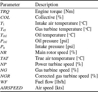
For the development and training of the data-driven MISO and SISO models, we utilised an extensive AW189 engine dataset consisting of time series data for key features of interest, as outlined in Table 1. Due to the specific configuration of the AW189 data acquisition system, all signal sampling frequencies are exact multiples of
 $8$
Hz. This property allows for efficient decimation while preserving the original dynamic characteristics of the signals. To prevent aliasing effects during the resampling process, a 20th-order low-pass finite impulse response (FIR) anti-aliasing filter is applied to continuous signals, preserving a bandwidth of up to
 $3.2$
Hz before uniformly downsampling all signals to
 $8$
Hz. The filtering process effectively smooths the signals, reducing high-frequency noise and enabling more stable and accurate numerical differentiation, a crucial requirement for the subsequent application of the SINDy algorithm.
List of variables

The dataset covers 196 individual flights and spans more than 35 hours of recorded flight time. Out of the 196 available flights in the dataset, 180 are used for the models’ development. These are further divided into a training dataset (
 ${D_{train}}$
) and a validation dataset (
 ${D_{val}}$
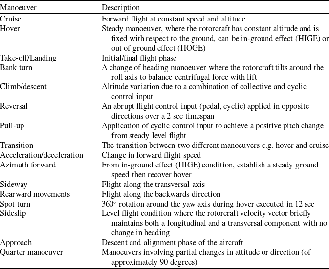
), consisting of 162 and 18 flights, respectively. These flights are never involved in the training phase and include a variety of standard manoeuvers listed and briefly described in Table 2. However, for the purpose of this analysis, some of the manoeuvers present in the original dataset, such as autorotations, normal shutdown, and taxiing, have little or no significance and were therefore excluded.
List of manoeuvers in the training and validation datasets

The remaining 16 flights form the test dataset (
 ${D_{test}}$
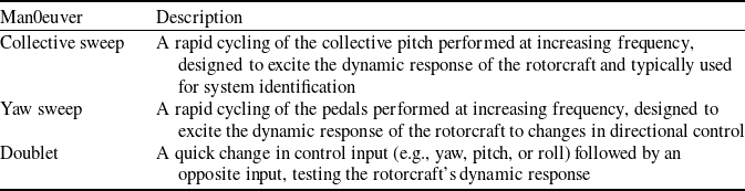
) used for the final evaluation of all models. These flights were not randomly selected. They specifically include high-frequency sweep manoeuvers, such as very fast collective and pedal inputs, which exhibit significantly more complex dynamic behaviour than those present in the training and validation datasets. As for the training and validation datasets, we present in Table 3 a list of the sweep manoeuvers, along with a brief description of each.
List of manoeuvers in the test dataset

Identical training and cross-validation phases are carried out for the MISO models and for SISO SINDy models by exploiting davinci-1 Footnote 2 , Leonardo S.P.A.’s High Performance Computing Facility and one of the most powerful supercomputers in the aerospace, defence and security sector.
As ML models rely on statistical analysis and are strongly influenced by the distribution and quality of the data, we performed a correlation analysis to identify highly and poorly correlated variables to be included and/or excluded from the training database (Fig. 5). The correlation between two features ranges between
 $ - 1$
and
 $ + 1$
. Features with a correlation coefficient of
 $1$
are directly correlated, while those with a correlation coefficient of
 $ - 1$
are inversely correlated. Features that are uncorrelated have values close to zero. Since datasets typically contain a large number of features describing each sample, analysing their correlations may help in selecting the most relevant features and discarding those that are not needed to build an effective predictive model. For instance, highly or poorly correlated features can cause multicollinearity in prediction models, a situation in which predictors are linearly dependent, potentially leading to bias in the results. In such cases, highly or poorly correlated features should be removed from the model’s input to reduce information redundancy in the data and potentially improving the model performance. In our case, for example,
 ${T_{45}}$
has a strong correlation (
 $0.86$
) with
 $TRQ$
, and is also closely related to the collective
 $COL$
(
 $0.87$
), which in turn shows a significant correlation with the torque (
 $0.79$
) as well. One approach would be to remove
 $COL$
from the list of inputs and consider only
 ${T_{45}}$
so to reduce the problem dimensionality. However, many of the variables that, as shown in Fig. 5, would be the best candidates, are not typically available for engine monitoring because they are internal to the engine itself. From a practical perspective, the aim of this work is to train a model for engine control using only information that is always accessible. In most cases, the engine manufacturer does not permit such detailed monitoring of the system, for obvious reasons related to intellectual property protection. This is why, despite the high correlation, variables like
 ${T_{45}}$
,
 $NG$
,
 ${T_{Oil}}$
, and
 ${P_{Oil}}$
cannot and should not be considered for model training, even though it is highly probable that some of these could lead to more accurate models.
Features correlation matrix for the engine variables used in the models in this paper.

Table 4 summarises the final set of variables included into the MISO input-output feature set after the analysis of Fig. 5.
MISO models input-output features set

The accuracy of all developed models is evaluated using the relative mean absolute error (
 $rMAE$
) index, where a lower value indicates better performance. This score is calculated for each manoeuver of interest in each flight using the following formula:
 \begin{align}rMA{E_i} = \frac{{MA{E_i}}}{{\overline {TR{Q_j}} }}\end{align}
where
 $MA{E_i}$
is the mean absolute error of the
 $i - th$
manoeuver of the
 $j - th$
flight and
 $\overline {TR{Q_j}} $
is the average
 $TRQ$
of that specific flight. Then, to provide an overall index to compare the accuracy of the training phases of each developed model, we first calculate the
 $rMA{E_j}$
, i.e., the average of the
 $rMA{E_i}$
scores for the
 $j - th$
flight and next global
 $rMAE$
score is obtained by averaging all the
 $rMA{E_j}$
.
3.0 Results and Discussion
To evaluate the capabilities of the developed data-driven models in describing the engine’s dynamic behaviour, the following sections compare the results obtained during the testing phase on the
 ${D_{test}}$
dataset, consisting of 16 flights. The best and worst results are presented by plotting the model predictions against the actual
 $TRQ$
values for these flights, each of which is uniquely identified by an ID (e.g., ID1, ID2, up to ID16). All the data in the figures are scaled in the range
 $\left[ {0,1} \right]$
with a Min-Max scaler.
3.1 MISO neural network results
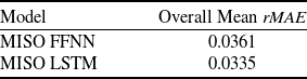
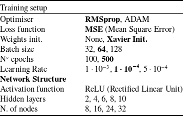
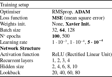
In this section, we present and analyse the performance of the MISO data-driven models by highlighting both the best and worst results obtained from the prediction of flight manoeuvers. Table 5 details the training setup of the two MISO data-driven models tuned through an extensive campaign of training and tests to determine the most suitable network structures, while Table 6 summarises the overall
 $rMAE$
indices for the training phase of each model. The best FFNN model consists of four hidden layers of 24 neurons each and the best LSTM model encodes three recurrent layers and a hidden size equal to 6. More details on the hyperparameter and network structure choices are given in Appendix 4.
MISO models training setup

Overall Training mean relative
 $MAE$
per model on the Validation set

Figures 6 and 7 present results obtained for two different manoeuvers of two different flights from the test set. In particular, Fig. 6 refers to flight ID1 and compares the
 $TRQ$
predictions of FFNN (
 $rMA{E_{FFNN}} = 3.75{\rm{\% }}$
) and LSTM (
 $rMA{E_{LSTM}} = 2.34{\rm{\% }}$
) with the normalised actual
 $TRQ$
. Although in terms of
 $rMAE$
per manoeuver the results obtained by the two MISO models may seem comparable, it is evident from the graph that FFNN is unable to capture the engine dynamics. In fact, its weakness emerges especially for manoeuvers (such as the collective sweep) in which the dynamic response of the engine is intentionally excited. A second problem is the lack of smoothness of the reconstructed
 $TRQ$
time series, which has a general ‘noisy’ and ‘spiky’ behaviour. The lack of smoothness is a direct consequence of network structure and architecture, where each time instant is treated in isolation without taking into account the time history of the input variables. On the contrary, the predictions of LSTMs fit the original signal better; their feedback connections allow them to handle the sequential nature of time series data, capturing long-term patterns and dependencies, which makes them ideal for predicting time series data.
Comparison of FFNN and LSTM predictions of normalised
 $TRQ$
for a manoeuver of Flight ID1 in the
 ${D_{test}}$
dataset.

Comparison of FFNN and LSTM predictions of normalised
 $TRQ$
for a manoeuver of Flight ID6 in the
 ${D_{test}}$
dataset.

Figure 7 is a second example of a comparison between the prediction results of MISO models and the normaliased real
 $TRQ$
. Again, it is evident that the LSTM network (
 $rMA{E_{LSTM}} = 1.82{\rm{\% }}$
) provides a better prediction of the dynamic behaviour of the
 $TRQ$
with respect to the FFNN (
 $rMA{E_{FFNN}} = 2.21{\rm{\% }}$
), which continues to produce a very noisy result and, more importantly, fails to capture sudden spikes in the measured TRQ.
Figures 8 and 9 show additional results for two different manoeuvers in the test set. The dynamic component appears to be well predicted, at least by the LSTM model, but in this case the predicted values seem to be consistently shifted by a constant. This suggests that the static component of the dynamics is not accurately captured.
Comparison of FFNN and LSTM predictions of normalised
 $TRQ$
for a manoeuver of Flight ID11 in the
 ${D_{test}}$
dataset.

Comparison of FFNN and LSTM predictions of normalised
 $TRQ$
for a manoeuver of Flight ID10 in the
 ${D_{test}}$
dataset.

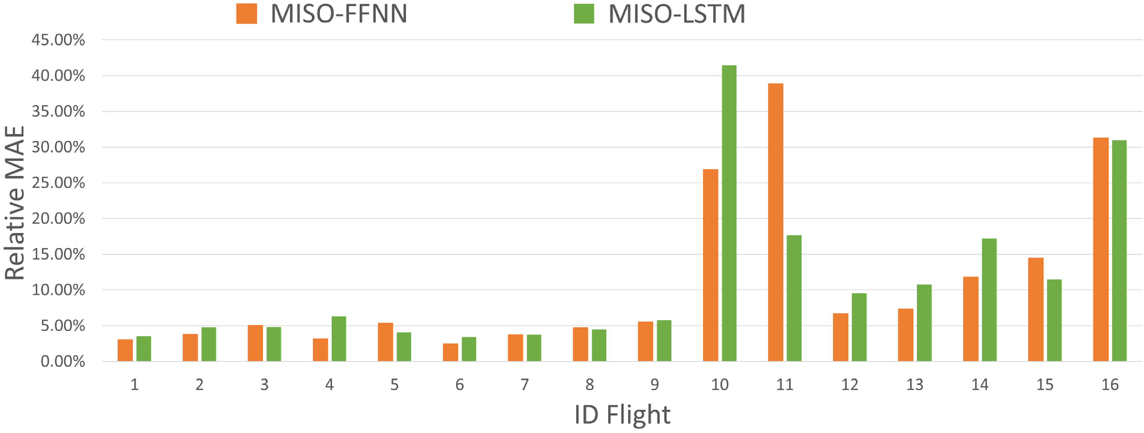
An analysis of the
 $rMAE$
scores per single test flight (Fig. 10) shows that, while for flights between ID1 and ID9 the
 $rMA{E_j}$
is acceptable and comparable to the training and testing scores, for the remaining flights (ID10 to ID15) the
 $rMA{E_j}$
is significantly larger, with
 $rMA{E_j}$
scores as high as 42.42%, because of a static offset of the predicted
 $TRQ$
.
MISO models
 $rMAE$
score per single test flight.

The causes of this behaviour can be related to errors and uncertainties in the collected flight data.
The data from flights ID1 to ID9 pertains to flight tests conducted in 2016, while flights ID10 to ID15 correspond to tests carried out in 2018. This two-year gap introduces potential changes in both the measurement system and the engine’s performance, which could affect the accuracy and generalisability of the machine learning model trained exclusively on the 2016 data. Over this period, it is possible that onboard sensors, including those used to measure torque or some input variables, may have undergone maintenance, recalibration, or even replacement, which could result in discrepancies in the data collected in 2018 compared to 2016. Furthermore, the engine may have experienced wear and tear, leading to alterations in its performance characteristics, including its torque response.
As components age and accumulate flight hours, their ability to perform at peak efficiency can degrade, leading to subtle but significant changes in the engine’s behaviour during flight tests. Moreover, not only the engine, but also the helicopter’s overall setup and other components, such as the rotor blades or transmission system, could have been replaced or modified over time. These changes in the airframe or mechanical systems could further affect the torque output and the overall performance of the helicopter. Unfortunately, we are unaware of the specific details regarding any replacements or modifications to the helicopter’s components between 2016 and 2018. This uncertainty complicates the model’s ability to account for all potential variations in the system, further emphasising the need for caution when applying the model to newer data. As a result, the machine learning model, which has been trained on data from a less-worn engine and potentially different components, might struggle to accurately predict torque values from a more aged system or modified helicopter. This issue highlights the importance of considering the evolving nature of the system when developing predictive models, as the model’s performance may degrade if it fails to account for changes in the instrumentation and the engine’s operational characteristics over time. Therefore, regular updates to the model, incorporating new data that reflects the current state of the engine and its components, are crucial to maintaining its accuracy and robustness.
Another potential cause for reduced prediction accuracy could be the absence of essential variables that are not included in the input feature set. For instance, the helicopter’s climb rate is a critical feature that directly impacts the torque response. Even at the same Collective Pitch (
 $COL$
), a higher climb rate generally results in a higher torque requirement due to the increased engine power demand on the engine as the helicopter ascends. The torque response can vary significantly depending on the rate of climb, as different flight profiles (such as steady, climbing or descending flights) impose distinct aerodynamic and mechanical stresses on the engine and rotor system.
All these hypotheses are supported by the relationship between the average
 $COL$
and average
 $TRQ$
per flight (Fig. 11): a discrepancy may be observed between the distribution of the training dataset and one of the test dataset. In fact, the majority of flights with the highest relative
 $MAEs$
do not fall within the distribution of training flights. Hence, neural networks struggle to accurately predict
 $TRQ$
because the training data do not cover these behaviours. To achieve greater accuracy in
 $TRQ$
prediction on
 ${D_{est}}$
flights, a new training phase of MISO models is performed by including 11
 ${D_{test}}$
flights in
 ${D_{train}}$
. The 11 test flights added to
 ${D_{train}}$
include both flights with ID1 to ID9 (for which the MISO models already work quite well) and flights with ID10 to ID15, which are not part of the initial training set.
Scatter plot of average
 $COL$
and
 $TRQ$
values for training/validation and test datasets. Red labels highlight the ID-FLIGHTS in the test set with hight
 $rMAE$
score.

By incorporating the test flights into the training set, MISO model performance improves; in fact, the scores obtained in the test phase after models re-training phase go from a
 $rMA{E_{FFNN}} = 13.50{\rm{\% }}$
to a
 $rMA{E_{FFNN}} = 5.78{\rm{\% }}$
and from a
 $rMA{E_{LSTM}} = 8.32{\rm{\% }}$
to a
 $rMA{E_{LSTM}} = 4.06{\rm{\% }}$
.
The performance improvements of the two MISO models are even more evident when looking at Fig. 12, which shows the same ID10 flight manoeuver as in Fig. 9. Even though the predictions are now mostly superimposed to the normalised real
 $TRQ$
, the FFNN model still fails in properly predicting high-frequency and small amplitude
 $TRQ$
oscillations for sweep flights.
Comparison of FFNN and LSTM predictions of normalised
 $TRQ$
for a manoeuver of Flight ID10 in the
 ${D_{test}}$
dataset after MISO models re-training.

3.2 SINDy Results
In this section, we present the results of the SINDy model training, which aims to identify the underlying dynamic relationships from the dataset. The following relation was obtained after selecting a polynomial candidate functions library:
 \begin{align}\dot TRQ\left( t \right) = - a - b{\rm{\;}}TRQ\left( t \right) + c{\rm{\;}}WF\left( t \right)\end{align}
where a, b and c are all positive coefficients and t is time. In fact, this result is not unexpected. In standard transfer-function modeling approaches, the
 $WF$
-
 $TRQ$
relation is modeled by a transfer function as follows:
 \begin{align}\frac{{TRQ\left( s \right)}}{{WF\left( s \right)}} = \frac{\mu }{{1 + \tau s}}\end{align}
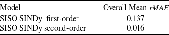
which may be easily reconducted to a first-order ODE in time domain. Even though this result shows how SINDy is able to correctly recover the system dynamics from data without previous knowledge of the underlying physics, the first order Equation (9) is not so useful in terms of accuracy, as intuitively shown by the overall mean
 $rMAE$
, reported in Table 5. The simulations are obtained for each manoeuver in
 ${D_{test}}$
by using as initial conditions the value of
 $TRQ$
at the beginning of the manoeuver itself, and then integrating in time via the time integration algorithm provided by PySINDy package. A step further is obtained by forcing a second-order model for SINDy prediction. The strategy is to modify the state and input vectors by including the time derivatives of
 $TRQ$
and
 $WF$
:
 \begin{align}{{\bf{X}}_{\bf{i}}} = \left( {\begin{array}{*{20}{l}}{TR{Q_{i1}}}\quad {}{TR{Q_{i2}}}\quad {}{TR{Q_{i3}}}\quad {} \ldots\quad {}{TR{Q_{i{m_i}}}}\\[6pt]{\dot TR{Q_{i1}}}\quad {}{\dot TR{Q_{i2}}}\quad {}{\dot TR{Q_{i3}}}\quad {} \ldots\quad {}{\dot TR{Q_{i{m_i}}}}\end{array}} \right)\end{align}
 \begin{align}{{\bf{U}}_{\bf{i}}} = \left( {\begin{array}{*{20}{l}}{W{F_{i1}}}\quad {}{W{F_{i2}}}\quad {}{W{F_{i3}}}\quad {} \ldots\quad {}{W{F_{i{m_i}}}}\\[6pt]{\dot W{F_{i1}}}\quad {}{\dot W{F_{i2}}}\quad {}{\dot W{F_{i3}}}\quad {} \ldots\quad {}{\dot W{F_{i{m_i}}}}\end{array}} \right)\\\nonumber\end{align}
so as to look for a system of equations instead.
In this case, the time-derivatives of the state and input signals are evaluated by numerical differentiation and are used to train SINDy model, leading to the following result
 \begin{align}\left\{ {\begin{array}{*{20}{l}}{\dot TRQ\left( t \right) = a'\dot TRQ}\\[5pt]{\ddot TRQ\left( t \right) = b'\dot TRQ\left( t \right) + c'\dot WF\left( t \right)}\end{array}} \right.\end{align}
where the first is clearly a dummy equation with
 $a{\rm{'}} = 1$
, which emerges naturally from the SINDy algorithm, while
 $b{\rm{'}}$
and
 $c{\rm{'}}$
are positive coefficients. It is interesting to point out that the dummy equation involving the coefficient
 $a{\rm{'}} = 1$
results directly from the algorithm, as the second-order model expands the state space by including the derivative of
 $TRQ$
. Nevertheless, since this is a dummy equation, the value of
 $a{\rm{'}}$
produced by the algorithm serves as a meaningful indicator of the quality of the regression. If it differs from the expected value of 1, it would suggest that the model fails to accurately represent the system–even when reconstructing a simple identity.
By using the second-order SINDy model given by system 13 to simulate the
 $TRQ$
time-histories of the test dataset, a significant improvement is obtained. As reported in Table 7, we obtain a reduction of one order of magnitude with respect to the first-order model in terms of overall mean relative
 $MAE$
. In this case, an additional initial condition is required on the
 $\dot TRQ$
, while the new input variable is the time-derivative of
 $WF$
.
Overall Training mean relative
 $MAE$
per SINDy model

At first glance, the very large difference between the two SINDy models may appear counterintuitive since the second equation of system 13 is easily traced back to a first-order model by integrating in time. Actually, we obtain
 \begin{align}\smallint \ddot TRQ\left( t \right) = \smallint - b'\dot TRQ\left( t \right)dt + \smallint c'\dot WF\left( t \right)dt\end{align}
leading to
 \begin{align}\dot TRQ\left( t \right) = - b'TRQ\left( t \right) + c'WF() + const\end{align}
which is the same expression as Equation (9). However, the coefficients resulting from the two different training processes are quite different, and the results provided by the second-order SINDy model are sufficiently accurate even for
 ${D_{val}}$
.
Before proceeding with the discussion of the result for the validation dataset, it should be noted that the SINDy model differs in a very important aspect from the FFNN and LSTM models presented in the previous paragraphs. The SINDy model takes only an internal variable of the system as input, while ignoring the real pilot control variables, namely collective (
 $COL$
) and main rotor speed (
 $NR$
). It follows that a direct comparison of SINDy
 ${2^{nd}}$
order scores with those of FFNN and LSTM may be misleading, as Equation (15) pertains only to a single engine component, providing a direct relation between
 $WF$
and
 $TRQ$
. Still, it is interesting to discuss the following results to demonstrate SINDy’s potential to extrapolate accurate physical models from normal flight data.
Figures 13 through 16 present the same flight manoeuvers discussed in subsection 3.1 for the MISO neural networks. It is clear that the simulation results obtained from Equation (13) are highly accurate, reproducing TRQ dynamics very well with only slight under/overestimations of some oscillation peaks. Again, an estimate of the total error is given by the rMAE score per test flight, which in this case is always lower than
 $3{\rm{\% }}$
. As anticipated above, these results demonstrate the potential of the SINDy approach in extrapolating a simple and interpretable dynamic model even without a deep understanding of the underlying physics of the system. However, in this case, the transition to the second order is crucial to achieve more than satisfactory accuracy. This behaviour, in our experience, is not easily predictable, as
 $WF$
-
 $TRQ$
relationship is typically modeled using transfer functions associated to
 ${\rm{first}}$
order ODE (see Equation (10)). It is likely that the information carried by the temporal derivative of fuel flow, the new control variable for the system of Equation (13), together with the additional initial condition on
 $\dot TRQ$
, may constitute the key for the improvement achieved in terms of model performance.
SINDy second-order prediction of normalised
 $TRQ$
for a manoeuver of Flight ID1 in the
 ${D_{test}}$
dataset.

SINDy second-order prediction of normalised
 $TRQ$
for a manoeuver of Flight ID6 in the
 ${D_{test}}$
dataset.

SINDy second=order prediction of normalised
 $TRQ$
for a manoeuver of Flight ID11 in the
 ${D_{test}}$
dataset.

SINDy second-order prediction of normalsed
 $TRQ$
for a manoeuver of Flight ID10 in the
 ${D_{test}}$
dataset.

4.0 Conclusions
In this paper, three different supervised data-driven approaches have been presented with the goal of developing a dynamic turboshaft engine model to extend the scope of commonly used transfer function-based and state-space perturbation models. The developed data-driven engine models have been trained, validated and tested on a database of real-flight tests of Leonardo’s AW189 prototypes and accurately predict the engine torque over the entire flight envelope of the helicopter, demonstrating that neural networks may effectively be used to simulate nonlinear behaviours of a helicopter engine. Specifically, two different MISO neural network architectures have been developed, namely a FFNN and a LSTM network, which take as input the time-histories of engine and environmental variables to predict the desired engine torque. The results show that the FFNN’s predictions lack accuracy and feature strong oscillations that are unacceptable for engine control. On the other hand, the LSTM, being a recurrent network, yields better predictions of
 $TRQ$
dynamic behaviour since its output is based on a time window that improves performance in terms of signal smoothness. The LSTM results are promising, but as shown by the analysis on the test dataset, which includes flights conducted long after the original training flights, the trained model lacks sufficient flexibility and fails to maintain satisfactory performance. As a consequence, a new training phase is necessary to update the model in response to the aircraft’s aging process. As future work, it would be of interest to further expand the dataset by including different aircraft types and flight campaigns, in order to evaluate whether more complex network architectures could generalise more effectively, thus leveraging the predictive capability demonstrated on the training and validation sets.
The predictive capability of purely data-driven neural network models, however, comes at a cost. Unlike physics-based approaches, they often act as ‘black boxes’, making it difficult to understand the underlying decision-making processes. This lack of transparency complicates diagnostics and compromises reliability, especially in safety-critical contexts. As a result, the trade-off between accuracy and interpretability remains a key issue in the adoption of such models, particularly in aerospace where explainability is essential for certification and trustworthiness. For this reason, with the intent of developing an interpretable ML dynamical model, we have used the SINDy approach to derive an accurate interpretable representation of the system dynamics directly from flight data even in the absence of a prior deep understanding of the underlying physics of the system. The obtained results, although preliminary as they focus on a specific engine component, show that the SISO SINDy model can effectively reproduce the
 $TRQ$
dynamics, but only when a second-order model is explicitly enforced within the SINDy algorithm. In this configuration, the SINDy model proves to be significantly more flexible than the purely data-driven neural network models analysed in this study, and the results demonstrate that its predictions remain highly accurate even on the test dataset, including sweep manoeuvers. Considering the encouraging results obtained with the SINDy model, future developments of this work will aim at extending the methodology to derive a complete engine model capable of predicting torque directly from real pilot control inputs.
Competing interests
The authors declare that they have no competing interests in relation to the work described in this manuscript.
Appendix
Hyperparameter Tuning and Training Setup
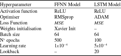
To determine the most suitable hyperparameters for the MISO data-driven models (e.g. number of layers, number of neurons, learning rate and batch size), we compared different network structures and training setups. Tables 8 and 9 present the hyperparameter grids for the FFNN and LSTM models, respectively. The best training setup parameters identified during training are highlighted in bold.
FFNN hyperparameter grid

LSTM hyperparameter grid

With the aim of illustrating the performance of the investigated FFNN structures and providing insights into the selection of the best architecture, Fig. 17 shows a table reporting the values of the mean absolute error (MAE) and the relative mean absolute error (rMAE) for both the Training and Validation datasets, along with the training time of each model, where the best architectures with the same number of nodes are highlighted with different colors. As expected, smaller networks show worse
Performance and training time of different FFNN structures. Training time is expressed in hours and minutes (hh:mm).

Validation loss vs training loss for different FFNN structures.

Performance and training time of different LSTM structures. Training time is expressed in hours and minutes (hh:mm).

Validation loss vs training loss for different LSTM structures.

performance in terms of rMAE. For instance, the first two structures, namely
 $2$
and
 $4$
hidden layers with
 $8$
nodes each, achieved an rMAE of
 $4.47{\rm{\% }}$
on the training set, which is significantly higher compared to larger networks. On the other hand, the largest model (
 $10$
hidden layers with
 $32$
nodes each) is clearly affected by overfitting. In fact, although the smallest rMAE was obtained on the training set (
 $2.69{\rm{\% }}$
), this was not the case for the validation set, where the model performed poorly with an rMAE of
 $3.93{\rm{\% }}$
. Again, this is an expected behaviour, as it is well known that larger machine learning models are often prone to overfitting issues. Figure 18 depicts this behaviour more clearly, reporting on the
 $x$
and
 $y$
axes the values of the loss function for the training set and the validation set, respectively. The best models should be the ones lying on the diagonal of the plane. The same analysis was done for the LSTM model. Figure 19 shows the performances of the different networks structure. First of all, looking at the last column, we notice that LSTM networks take much longer to train than feed-forward NN networks (Fig. 17). Second, in general LSTM networks obtain greater accuracy: in fact, while the relative MAE of feed-forward networks is on average around
 $3.8{\rm{\% }}$
, here the relative MAE of LSTM networks is on average equal to
 $3.5{\rm{\% }}$
. The best performing networks are the ones highlighted in colors, which have a relative MAE of about
 $3.3{\rm{\% }}$
for the training set around and about
 $3.4{\rm{\% }}$
for the test set. The scatter plot of the loss functions in Fig. 20 also confirms that LSTM models have greater accuracy than feed-forward networks. In fact, the points of the different networks in the chart are more aligned along the diagonal, showing less tendency of overfitting and lower loss values. The network that has the highest accuracy is the one characterised by
 ${\rm{four}}$
recurrent layers and a hidden size equal to
 ${\rm{six}}$
, with an rMAE equal to
 $3.30{\rm{\% }}$
on the validation set. However, the performance increase of this network structure compared to the one with
 ${\rm{three}}$
recurrent layers and
 ${\rm{six}}$
as hidden size is only
 $1.5{\rm{\% }}$
, while the computational cost increases by more than
 $30{\rm{\% }}$
. For this reason, the latter architecture was considered the optimal one for the study presented in this work.