
 10∘
 0∘
 20∘
 40∘





1. Introduction
1.1. Motivation
Hypersonic flight inevitably entails the formation of strong shocks ahead of flying bodies. These shocks compress the free stream and generate high-temperature, high-density flow fields in front of the vehicle, within which boundary layers develop along the surface. In hypersonic flows, boundary-layer dynamics play a critical role in determining surface heating and skin friction. Accordingly, their stability (Knisely & Zhong Reference Knisely and Zhong2019; Roy & Scalo Reference Roy and Scalo2026), turbulent transition (Xu et al. Reference Xu, Wang and Chen2022; Sousa et al. Reference Sousa, Wartemann, Wagner and Scalo2024; Schuabb et al. Reference Schuabb, Duan, Casper, Wagnild, Choudhari and Paredes2025) and fully turbulent states (Renzo & Urzay Reference Renzo and Urzay2021; Huang et al. Reference Huang, Duan and Choudhari2022; Passiatore et al. Reference Passiatore, Sciacovelli, Cinnella and Pascazio2022; Toki et al. Reference Toki, Sousa, Chen, Camillo, Wagner and Scalo2025; Williams et al. Reference Williams, Renzo and Moin2025) have been intensively investigated using high-fidelity numerical approaches such as direct numerical simulations and large-eddy simulations. These studies mainly focus on the near-wall physics under prescribed post-shock conditions. However, in high-enthalpy regimes, strong shock-layer processes can substantially modify the flow upstream of the boundary layer, generating vorticity that subsequently evolves in the post-shock region. Indeed, it has been reported that upstream conditions can significantly influence downstream boundary-layer behaviour (Sousa et al. Reference Sousa, Wartemann, Wagner and Scalo2024). Despite this extensive body of work on hypersonic boundary layers, the fluid dynamics of the shock layer, particularly the vorticity generation and evolution in the immediate post-shock region, remain incompletely understood.
Unless the leading edge of a flying body is perfectly sharp, a detached curved shock forms ahead of the vehicle. In high-enthalpy regimes close to practical flight conditions, the specific total enthalpy can reach values of the order of
 $10\,\mathrm{MJ\,kg^{-1}}$
, corresponding to total temperatures of approximately
 $10\,000\,\mathrm{K}$
. The detached curved shock produces strong compression and high post-shock temperatures, which lead to the dissociation and ionisation of air (Gnoffo et al. Reference Gnoffo, Gupta and Shinn1989; Park Reference Park1990). Recent computational studies have focused on accurate modelling of ionisation (Boyd & Josyula Reference Boyd and Josyula2021; Munafò & Panesi Reference Munafò and Panesi2025) and species diffusion (Amato & Candler Reference Amato and Candler2023), which are essential for simulating practical or experimental conditions (Gibbons et al. Reference Gibbons, Damm and Gollan2021; Aiken & Boyd Reference Aiken and Boyd2024; Munafò et al. Reference Munafò, Stephani and Panesi2025). In parallel, high-enthalpy wind-tunnel experiments have been extensively conducted (Ananthapadmanaban et al. Reference Ananthapadmanaban, Wallington, Hopkins, Gibbons, Toki, Scalo, Gildfind, James, Mee and Veeraragavan2024; Aiken et al. Reference Aiken, Boyd, Paxton and McGilvray2026; Chander & Maddalena Reference Chander and Maddalena2026), providing data that are compared with simulations.
These studies have significantly advanced the understanding of high-enthalpy shock-layer chemistry and transport processes, enabling accurate prediction of ionisation effects on radiative heating and electromagnetic interference. On the other hand, comparatively little attention has been paid to the vorticity generated within and immediately downstream of curved shocks. In hypersonic flows, shock curvature, aerothermochemical effects and compressibility can jointly generate and amplify vorticity, which subsequently evolves in the post-shock region and can strongly influence downstream boundary-layer development, including transition and surface heat transfer. Such vorticity can also affect quantities of practical interest, such as the stagnation heat flux (Marineau et al. Reference Marineau, Lewis, Smith, anb Molly, Lafferty and Amar2013). Early theoretical studies of dissociating flows were conducted by Lighthill (Reference Lighthill1957), who introduced an ideal dissociating-gas framework to examine the effects of chemical reactions on shock-wave properties. Subsequently, Wu & Hayes (Reference Wu and Hayes1958) and Hayes & Probstein (Reference Hayes and Probstein1966) provided kinematic descriptions of vorticity production across curved shocks in such reactive environments. Despite these foundational contributions, existing discussions of vorticity generation at a curved shock are largely limited to theoretical analyses, as summarised in § 1.2. To the authors’ knowledge, vorticity generation and its subsequent evolution in the post-shock region have not yet been systematically investigated using experiments or numerical simulations.
Therefore, the present paper focuses on vorticity generation at a curved shock and the resulting vorticity field in the post-shock region, based on numerical simulations incorporating aerothermochemical modelling, with particular emphasis on the roles of fluid dissociation and wedge angle. In addition, selected results are compared with available high-enthalpy wind-tunnel measurements to assess whether the simulations reproduce the experimentally observed trends associated with variations in free-stream composition.
1.2. Theoretical analysis of vorticity generation at a curved shock
Several analytical relations relevant to hypersonic flows have been derived in the literature. In this section, those necessary to discuss vorticity generation at a curved shock are summarised and rederived for completeness. Figure 1 illustrates the configuration and coordinate system considered.
Sketch of a curved shock including aerothermochemical effects with dissociation of
 $\mathrm{O_2}$
and
 $\mathrm{N_2}$
into
 $\mathrm{O}$
,
 $\mathrm{N}$
and
 $\mathrm{NO}$
. Here
 $U_{\infty }$
denotes the free-stream velocity. The coordinates
 $\xi$
and
 $\eta$
are defined along the streamline and the curved shock, respectively. The velocity components
 $u$
and
 $v$
are taken in the
 $\eta$
direction and in the direction normal to it. The angles
 $\sigma$
and
 $\theta$
denote the shock inclination and the streamline direction measured from the free-stream direction, respectively.

For a non-reacting ideal gas, Crocco derived a relation between the vorticity
 $\boldsymbol{\zeta }$
generated by a curved shock and the specific entropy
 $S$
under steady conditions (von Kármán Reference von Kármán1954). Wu & Hayes (Reference Wu and Hayes1958) extended Crocco’s equation to reacting inviscid flows, and Emanuel (Reference Emanuel2007) generalised the equation for unsteady and viscid flows. Here, the derivation for reacting inviscid flow is provided, and it starts from the three-dimensional inviscid momentum equation
 \begin{align} \rho (\boldsymbol{u}\boldsymbol{\cdot }\boldsymbol{\nabla })\boldsymbol{u}=-\boldsymbol{\nabla }\!p, \end{align}
where
 $\rho$
is density,
 $p$
is pressure and
 $\boldsymbol{u}$
is the velocity vector. The left-hand side of the equation can be rewritten as
 \begin{align} \rho (\boldsymbol{u}\boldsymbol{\cdot }\boldsymbol{\nabla })\boldsymbol{u}=\rho \left (\boldsymbol{\nabla }\left (\frac {1}{2}(\boldsymbol{u} \boldsymbol{\cdot }\boldsymbol{u}) \right ) - \boldsymbol{u}\times \boldsymbol{\zeta } \right )\!. \end{align}
Here,
 $\boldsymbol{\zeta } \equiv \boldsymbol{\nabla }\times \boldsymbol{u}$
is the vorticity. The right-hand side of (1.1) can be rewritten using the differential state equation
 \begin{align} {\rm d}h = T {\rm d}S + \frac {{\rm d} p}{\rho } +\sum _{\alpha } \mu _{\alpha } {\rm d}Y_{\alpha }, \end{align}
where
 $h$
and
 $T$
are the specific enthalpy and translational–rotational temperature, respectively. The subscript
 $\alpha$
indicates the specific species, and
 $\mu _{\alpha }$
and
 $Y_{\alpha }$
are the chemical potential and mass fraction of species
 $\alpha$
. The
 $h$
and
 $\mu _{\alpha }$
are defined by
 $\alpha$
-species specific enthalpy
 $h_{\alpha }$
and specific entropy
 $S_{\alpha }$
:
 \begin{align} h = \sum _{\alpha } h_{\alpha } Y_{\alpha }, \\[-28pt] \nonumber \end{align}
 \begin{align} \mu _{\alpha } = h_{\alpha } - T S_{\alpha }. \\[0pt] \nonumber \end{align}
Using the differential state equation, one obtains
 \begin{align} \frac {\boldsymbol{\nabla }\!p}{\rho }=\boldsymbol{\nabla }h -T \boldsymbol{\nabla }S - \sum _{\alpha } \mu _{\alpha } \boldsymbol{\nabla }Y_{\alpha }. \end{align}
Substituting (1.2) and (1.6) into the momentum equation (1.1), it can be written as
 \begin{align} \boldsymbol{u} \times \boldsymbol{\zeta } = \boldsymbol{\nabla }\left (h+\frac {1}{2}(\boldsymbol{u} \boldsymbol{\cdot }\boldsymbol{u})\right ) - T\boldsymbol{\nabla }S - \sum _{\alpha } \mu _{\alpha } \boldsymbol{\nabla }Y_{\alpha }. \end{align}
Since the total enthalpy is constant in the absence of external forces or energy sources, the gradient of the first term on the right-hand side vanishes. Thus, Crocco’s equation can be derived as
 \begin{align} \boldsymbol{u} \times \boldsymbol{\zeta } = - T\boldsymbol{\nabla }S - \sum _{\alpha } \mu _{\alpha } \boldsymbol{\nabla }Y_{\alpha }. \end{align}
To consider the effects of chemical reaction on vorticity, we mathematically analyse this equation for a two-dimensional flow prior to conducting numerical simulations. In this analysis,
 $\eta$
denotes coordinates along the curved shock. The velocity components in the
 $\eta$
direction and the perpendicular one are defined as
 $u$
and
 $v$
, respectively. Using the oblique shock relations, the velocity components downstream of the shock can be written as
 \begin{align} u_s = U_{\infty } \cos \sigma , \\[-28pt] \nonumber \end{align}
 \begin{align} v_s = U_{\infty } \cos \sigma \tan (\sigma - \theta _s) = U_{\infty }\frac {\rho _{\infty }}{\rho _s} \sin \sigma , \\[0pt] \nonumber \end{align}
where
 $U_{\infty }$
is the free-stream velocity,
 $\sigma$
is the inclination angle of the shock with respect to the free-stream direction and
 $\theta$
is the angle of the streamlines. The subscripts
 $\infty$
and
 $s$
indicate the free-stream and post-shock conditions, respectively. If we assume that a chemical reaction does not occur inside the shock, derivatives of a given mass fraction in the
 $\eta$
direction can be negligible immediately downstream of the shock
 $(\partial Y_{\alpha }/\partial \eta )_s = 0$
. When this assumption is adopted, (1.8) gives the following relation for the out-of-plane vorticity component
 $\zeta _s$
immediately downstream of the shock:
 \begin{align} \zeta _s U_{\infty } \frac {\rho _{\infty }}{\rho _s} \sin \sigma = T_s \left (\frac {\partial S}{\partial \eta } \right )_s = T_s \frac {{\rm d} S_s}{{\rm d} \eta }. \end{align}
In this paper, the counter-clockwise direction is taken as positive for vorticity.
On the other hand, when the free stream is uniform, all variables immediately downstream of the shock depend on only the shock angle
 $\sigma$
. In addition, since
 $Y_{\alpha , s}$
immediately downstream of the shock should be the same as the free stream at any shock location,
 ${\rm d}Y_{\alpha , s}/{\rm d} \sigma$
is 0. Thus, from (1.3), the differential equation downstream of the shock can be obtained as
 \begin{align} \frac {{\rm d}h_s}{{\rm d} \sigma } = T_s \frac {{\rm d}S_s}{{\rm d} \sigma } + \frac {1}{\rho _s}\frac {{\rm d}p_s}{{\rm d} \sigma }. \end{align}
The oblique shock relations are the same as for non-reacting flows. Using conservation of mass, momentum and energy, one obtains the following two relations:
 \begin{align} p_s -p_{\infty }=\left ( \frac {1}{\rho _{\infty }} -\frac {1}{\rho _s} \right )(\rho _{\infty } u_{\infty } \sin \sigma )^2, \\[-28pt] \nonumber \end{align}
 \begin{align} h_s - h_{\infty } = \frac {1}{2} \left ( 1-\frac {{\rho _{\infty }}^2}{{\rho _{s}}^2} \right ) \left (u_{\infty } \sin \sigma \right )^2. \\[0pt] \nonumber \end{align}
Differentiating these equations with respect to
 $\sigma$
and substituting them into (1.12), one obtains
 \begin{align} T_s \frac {{\rm d}S_s}{{\rm d} \sigma } = \left (1 - \frac {\rho _{\infty }}{\rho _s} \right )^2 {u_{\infty }}^2 \sin \sigma \cos \sigma . \end{align}
Dividing (1.11) by (1.15), we can obtain the following vorticity relation:
 \begin{align} \zeta _s = u _{\infty } \frac {\rho _s}{\rho _{\infty }} \left ( 1- \frac {\rho _{\infty }}{\rho _s} \right )^2 \cos \sigma \frac {{\rm d} \sigma }{{\rm d} \eta } .\end{align}
This relation was originally derived by Truesdell (Reference Truesdell1952) for non-reacting flows, and was later shown by Hornung (Reference Hornung1998) to remain valid for reacting flows, provided that chemical reactions advance negligibly across the shock.
1.3. Paper outline
The remainder of the paper is organised as follows. The numerical flow conditions are summarised in § 2, including the experimental conditions used for comparison. The computational set-ups are described in § 3, and results obtained from the present simulations are compared with experiments in § 4. Grid sensitivity analyses are provided in § 5. The main results of this study are presented in § 6, with the effects of wedge angle and fluid composition discussed separately in §§ 6.1 and 6.2, respectively. Finally, the findings are summarised in § 7.
2. Experimental and numerical flow conditions
The numerical study presented here is based on the operating conditions of the T4 Stalker Tube (a free-piston, reflected shock tunnel) at The University of Queensland (Mee et al. Reference Mee, Morgan, Paull, Jacobs and Smart2017). The T4 Stalker Tube operates over a wide range of conditions, enabling the reproduction of flight-equivalent states at altitudes of 10–32 km, with free-stream Mach numbers between 5 and 12 and specific total enthalpies between
 $1.5$
and
 $10\,\mathrm{MJ\,kg^{-1}}$
. The configuration considered is a two-dimensional high-enthalpy hypersonic flow over a blunt wedge, with a 5 mm nose radius, as shown in figure 2. The Cartesian coordinates
 $X$
and
 $Y$
denote the horizontal and vertical directions, respectively. The origin
 $(X,Y)=(0\,\mathrm{mm},0\,\mathrm{mm})$
is defined at the leftmost point of the rounded leading edge of the wedge, and the centre of the rounded leading edge is located at
 $(X,Y)=(5\,\mathrm{mm},0\,\mathrm{mm})$
. The flat portion of the wedge extends
 $200\,\mathrm{mm}$
downstream. To investigate the effects of wedge blockage, the wedge angle
 $\phi$
relative to the free-stream direction is varied between
 $0^\circ$
,
 $20^\circ$
and
 $40^\circ$
. In addition, a configuration with a shorter flat length of
 $100\,\mathrm{mm}$
and a wedge angle of
 $10^\circ$
is simulated for direct comparison with experiments conducted in the T4 Stalker Tube. The wedge tip produces a detached bow shock upstream of the stagnation point.
Computational configuration of hypersonic 2-D wedge with aerothermochemistry. The sponge boundaries are marked by blue dashed lines.

The simulated cases are summarised in tables 1 and 2. Here,
 $M$
denotes the Mach number and other symbols are defined in § 1.2. The subscript
 $\infty$
indicates free-stream conditions. Table 1 lists the cases used for comparison with the experiments presented in § 4. These cases are used to assess whether the simulations reproduce the experimentally observed trends associated with variations in free-stream composition. Under the experimental high-enthalpy conditions, dissociation of the working gas occurs, significantly altering the free-stream composition. The free-stream conditions for the cases in table 1 are obtained using NENZF1d (Gibbons et al. Reference Gibbons, Damm, Jacobs and Gollan2023). NENZF1d models the compression of the test gas in the shock tube to match the pressure in the nozzle-supply region measured in the experiment. The non-equilibrium flow of the test gas through the nozzle is then modelled as a quasi-one-dimensional expansion with finite rate chemical reactions modelled. The expansion continues until the ratio of the Pitot pressure to the nozzle-supply pressure from the calculations matches the ratio measured in nozzle calibration tests. These conditions are imposed as inflow boundary conditions in the present simulations. The case label specifies the wedge angle and the initial gas composition. The 10deg-N2 case consists of pure nitrogen, whereas the 10deg-Air case corresponds to an air composition and, therefore, experiences stronger dissociation than the 10deg-N2 case. In the 10deg-N2/O2-Mix case, a small amount of oxygen is added to nitrogen, resulting in intermediate reaction levels.
Experimental conditions at the T4 Stalker Tube used for comparison with numerical predictions.

Table 1. Long description
A table comparing experimental conditions for different gas compositions and their effects on free-stream properties. The table has 3 rows and 10 columns. Column headers are: Case, phi, p_infinity (Pa), T_infinity (K), rho_infinity (kg/m^3), U_infinity (m/s), M_infinity, Y_N2_infinity, Y_O2_infinity, Y_NO_infinity, Y_O_infinity. Row 1: 10deg-Air, 10 degrees, 20477 Pa, 1620 K, 0.042 kg/m^3, 4007 m/s, 5.01, 0.736, 0.156, 0.067, 0.000, 0.042. Row 2: 10deg-N2, 10 degrees, 18659 Pa, 1742 K, 0.036 kg/m^3, 4322 m/s, 5.24, 0.993, 0.0, 0.0, 0.007, 0.0. Row 3: 10deg-N2/O2-mix, 10 degrees, 18447 Pa, 1544 K, 0.040 kg/m^3, 4083 m/s, 5.20, 0.868, 0.055, 0.041, 0.000, 0.036.
List of computational cases with three wedge angles and five gas compositions. The N/A indicates that the corresponding case does not compute conservation of species.

Table 2. Long description
A table with 12 rows and 10 columns comparing computational cases with three wedge angles and five gas compositions. The columns are labeled as Case, φ, p∞ (Pa), T∞ (K), ρ∞ (kgm⁻³), U∞ (ms⁻¹), M∞, htotal,∞ (MJkg⁻¹), YN2,∞, and YO2,∞. The rows list different cases with varying wedge angles (0 degrees, 20 degrees, and 40 degrees) and gas compositions (Perfect-gas, N2-100, Air, N2-O2-50, and O2-100). The table includes values for each case under the respective columns, with some cells marked as N/A indicating that the corresponding case does not compute conservation of species.
The cases summarised in table 2 are used to examine the effects of aerothermal chemistry and wedge angle, as discussed in § 6. For these cases, the inflow pressure, temperature and velocity are identical, while the free-stream composition consists of diatomic nitrogen (
 $\mathrm{N_2}$
) and diatomic oxygen (
 $\mathrm{O_2}$
). The mass fraction of
 $\mathrm{O_2}$
is varied from
 $0\,\%$
to
 $100\,\%$
to control the strength of chemical reactions. In addition, a calorically perfect gas case without aerothermal chemistry is simulated for comparison. Here, a calorically perfect gas implies that the specific heat is independent of temperature. Despite identical inflow velocity and temperature, the free-stream Mach number and the specific total enthalpy,
 $h_{total,\infty }$
, vary slightly among the cases due to differences in specific heat. The free-stream Mach number ranges from 5.32 to 5.91 and the specific total enthalpy is approximately
 $9.15\,\mathrm{MJ\,kg^{-1}}$
, which is close to the upper limit of the T4 Stalker Tube. With three wedge angles and five free-stream gas compositions considered for each angle, a total of 15 cases are simulated.
The wedge walls are treated as adiabatic slip-wall boundaries to isolate vorticity generation to that associated solely with the bow shock; consequently, no boundary layer forms. A hypersonic inflow condition is imposed at the left curved boundary, while the upper and lower straight boundaries are treated as outlets. Sponge layers are applied at both the inlet and the outlets, where all flow variables are gradually relaxed toward the prescribed inflow conditions. The thickness of each sponge layer is determined based on the number of grid points, with each layer occupying 5 % of the grid points in the corresponding direction. The sponge-layer regions are indicated by blue dashed lines in figure 2. The computational grid is designed to be aligned with the bow shock. For the cases listed in table 1, the grid consists of
 $N_x = 512$
points in the shock-aligned direction and
 $N_y = 256$
points in the shock-normal direction. For the cases summarised in table 2, the grid resolution is
 $N_x \times N_y = 1024 \times 256$
. A separate shock-aligned mesh is generated for each simulation case to account for variations in free-stream conditions and the resulting shock geometry. A grid-refinement study is conducted for the 20deg-Air and 40deg-Air cases, and the results are presented in § 5.
3. Computational set-up
3.1. Governing equations
The simulations are performed by solving the two-dimensional conservation equations for mass, momentum, total energy and species mass. The governing equations are generalised following the formulation of Jordan (Reference Jordan1999) and Nagarajan et al. (Reference Nagarajan, Lele and Ferziger2007). In the present configuration, a structured grid defined in the physical space
 $\boldsymbol{y}$
is transformed into the computational space
 $\boldsymbol{x}$
,
 \begin{eqnarray} x^i & = & x^i(y_1,y_2), \\[-28pt] \nonumber \end{eqnarray}
 \begin{eqnarray} y_i & = & y_i \big(x^1,x^2 \big), \\[0pt] \nonumber \end{eqnarray}
where
 $x^i$
and
 $y_i$
denote the
 $i$
th coordinates in the computational and physical spaces, respectively. The governing equations are written as
 \begin{align} \frac {\partial J \rho }{\partial t} + \frac {\partial }{\partial x^j} \big(J \rho v^j \big)= 0, \\[-28pt] \nonumber \end{align}
 \begin{align} \frac {\partial J \rho v^i}{\partial t} + \frac {\partial }{\partial x^j} \big(J \rho v^i v^j + J p g^{\textit{ij}} - J \sigma ^{\textit{ij}} \big)= -\varGamma ^i_{qj} \big(J \rho v^q v^j + J p g^{qj} - J \sigma ^{qj} \big), \\[-28pt] \nonumber \end{align}
 \begin{align} \frac {\partial J E}{\partial t} + \frac {\partial }{\partial x^j} \left(J(E + p) v^j + J Q^{j} + \sum _{\alpha } N^j_{\alpha } h_{\alpha } \right)= \frac {\partial }{\partial x^k} \big(J \sigma ^{\textit{ij}}g_{ik} v^k \big), \\[-28pt] \nonumber \end{align}
 \begin{align} \frac {\partial J \rho Y_{\alpha }}{\partial t} + \frac {\partial }{\partial x^j} \big(J \rho Y_{\alpha } v^j + J N^{\kern-1pt j}_{\alpha } \big)= w_{\alpha }. \\[0pt] \nonumber \end{align}
Here,
 $J$
is the Jacobian of the transformation, defined as the determinant of the Jacobian matrix
 $J_{\textit{ij}}=\partial y_i/\partial x^j$
,
 $w_{\alpha }$
is the production rate of species
 $\alpha$
,
 $h_{\alpha }$
is the specific enthalpy of species
 $\alpha$
,
 $E$
is the total energy and
 $t$
denotes time. To isolate the effects of dissociation, radiative processes are neglected in the present analysis. The transformation between the physical velocity components
 $u_i$
and the contravariant velocity components
 $v^i$
is given by
 \begin{align} v^j = u_i \frac {\partial x^j}{\partial y_i}. \end{align}
In (3.3)–(3.6),
 $g_{\textit{ij}}$
and
 $g^{\textit{ij}}$
are the covariant and contravariant metric tensors, respectively, and
 $\varGamma ^i_{qj}$
denotes the Christoffel symbol of the second kind. These quantities are defined as
 \begin{align} g_{\textit{ij}} = \frac {\partial y_i}{\partial x^k}\frac {\partial y_j}{\partial x^k}, \\[-28pt] \nonumber \end{align}
 \begin{align} g^{\textit{ij}} = \frac {\partial x^k}{\partial y_i}\frac {\partial x^k}{\partial y_j}, \\[-28pt] \nonumber \end{align}
 \begin{align} \varGamma ^i_{qj} = \frac {\partial x^i}{\partial y_l}\frac {\partial ^2 y_l}{\partial x^q \partial x^j}. \\[-12pt] \nonumber \end{align}
In the curvilinear coordinate system, the viscous stress tensor
 $\sigma ^{\textit{ij}}$
, the heat-flux vector
 $Q^j$
and the diffusive mass flux of species
 $\alpha$
,
 $N^j_{\alpha }$
, are expressed as
 \begin{align} \sigma ^{\textit{ij}} = \mu \left ( g^{jk} \frac {\partial v^i}{\partial x^k} + g^{ik} \frac {\partial v^j}{\partial x^k} - \frac {2}{3} g^{\textit{ij}} \frac {\partial v^k}{\partial x^k} \right ) + \beta _{\textit{art}} g^{\textit{ij}} \frac {\partial v^k}{\partial x^k}, \\[-28pt] \nonumber \end{align}
 \begin{align} Q^j = - (\lambda + \theta _{\textit{art}}) g^{\textit{ij}} \frac {\partial T}{\partial x^i}, \\[-28pt] \nonumber \end{align}
 \begin{align} N^j_{\alpha } = - \rho D_{\alpha } \frac {M_{\alpha }}{M_{\textit{mix}}} g^{\textit{ij}} \frac {\partial X_{\alpha }}{\partial x^i}. \\[-12pt] \nonumber \end{align}
Here,
 $\mu$
is the viscosity coefficient,
 $\lambda$
is the thermal conductivity,
 $X_{\alpha }$
is the molar fraction of species
 $\alpha$
, and
 $M_{\textit{mix}}$
and
 $M_{\alpha }$
are the molecular weights of the mixture and species
 $\alpha$
, respectively. The diffusive mass flux is evaluated using the Hirschfelder–Curtiss approximation (Poinsot & Veynante Reference Poinsot and Veynante2012). The effective diffusion coefficient
 $D_{\alpha }$
is defined as
 \begin{align} D_{\alpha } = \frac {1-Y_{\alpha }}{\sum _{\beta \neq \alpha } X_{\beta } / \mathcal{D}_{\alpha \beta }}, \end{align}
where
 $\mathcal{D}_{\alpha \beta }=\mathcal{D}_{\beta \alpha }$
is the binary diffusion coefficient of species
 $\alpha$
into species
 $\beta$
. In the present simulations, all binary diffusion coefficients are assumed equal,
 $\mathcal{D}_{\alpha \beta }=\mathcal{D}$
, and are related to the Schmidt number
 $Sc$
by
 \begin{align} \mathcal{D} = \frac {\mu }{\rho Sc}. \end{align}
To stabilise the solution in the presence of strong shocks, a shock-capturing method is employed. Artificial bulk viscosity
 $\beta _{\textit{art}}$
is added to the dilatational component of the viscous stress tensor, and artificial thermal conductivity
 $\theta _{\textit{art}}$
is introduced in the heat flux. Details of the shock-capturing method are provided in § 3.2.
The total energy
 $E$
in (3.5) is defined as
 \begin{align} E = \frac {1}{2}\rho u_i u_i + \sum _{\alpha } \rho Y_{\alpha } e_{\alpha }, \end{align}
where
 $e_{\alpha }$
is the specific internal energy of species
 $\alpha$
, given by
 \begin{align} e_{\alpha } = \int _{T_{\textit{ref}}}^{T} C_v^{\alpha } \, \mathrm{d}T + e_{\alpha ,0}. \end{align}
Here,
 $C_v^{\alpha }$
is the specific heat at constant volume and
 $e_{\alpha ,0}$
is the formation energy of species
 $\alpha$
at the reference temperature
 $T_{\textit{ref}}$
. Similarly, the specific enthalpy of species
 $\alpha$
is expressed as
 \begin{align} h_{\alpha } = \int _{T_{\textit{ref}}}^{T} C_p^{\alpha } \, \mathrm{d}T + h_{\alpha ,0}, \end{align}
where
 $C_p^{\alpha }$
is the specific heat at constant pressure and
 $h_{\alpha ,0}$
is the formation enthalpy. These quantities satisfy
 \begin{align} h_{\alpha ,0} = e_{\alpha ,0} + \frac {\overline {R}}{M_{\alpha }} T_{\textit{ref}}, \\[-28pt] \nonumber \end{align}
 \begin{align} C_p^{\alpha } = C_v^{\alpha } + \frac {\overline {R}}{M_{\alpha }}, \\[0pt] \nonumber \end{align}
where
 $\overline {R}$
is the universal gas constant. The formation enthalpy
 $h_{\alpha ,0}$
for each species is listed in table 3.
Formation enthalpies of the species (McBride et al. Reference McBride, Zehe and Gordon2002). Values are converted from the reference units of
 $\mathrm{kJ\,mol^{-1}}$
using the molecular weight of each species.

Table 3. Long description
A table comparing formation enthalpies of different species. The table has 2 rows and 6 columns. The columns are labeled Species, N 2, O 2, NO, N, and O. The row labels are Species and h sub alpha comma 0 (k J kg superscript negative 1). Row 1: Species, h sub alpha comma 0 (k J kg superscript negative 1). Row 2: N 2, 0; O 2, 0; NO, 3042.4; N, 16881.4; O, 7786.7.
3.2. Numerical methods
The governing equations are solved using the sixth-order compact finite-difference code VAMPIRE (Zhao & Scalo Reference Zhao and Scalo2020), originally developed for incompressible flows (Zhao et al. Reference Zhao, Yu, Chapelier and Scalo2021). It has been extended to compressible flows following the numerical methodology of CFDSU, which has been successfully applied to several hypersonic cases (Chen & Scalo Reference Chen and Scalo2021; Sousa et al. Reference Sousa, Wartemann, Wagner and Scalo2024; Toki et al. Reference Toki, Sousa, Chen and Scalo2024). While the cited studies focused on non-reacting flows, the present work further incorporates aerothermochemistry. Experimental comparisons are performed for three representative cases using measurements from the T4 Stalker Tube (§ 4) to assess the predicted trends associated with variations in free-stream composition. Additional assessment of the thermochemical implementation is provided in Appendix A. Species molar fractions along a stagnation streamline are compared with results from an independent high-enthalpy reacting-flow solver, and the thermochemical coupling is further assessed through an enthalpy-budget analysis along a representative streamline. Together, these assessments indicate that the present implementation consistently captures the dominant thermochemical evolution and the associated energy redistribution.
Although VAMPIRE supports block-structured adaptive mesh refinement (AMR), this capability is disabled in the present study to maintain a consistent mesh hierarchy. The grid convergence assessment is based on a sequence of uniformly refined meshes, whereas AMR introduces non-uniform mesh distributions that may hinder a straightforward comparison of solutions across resolutions. The solver employs a staggered finite-difference scheme: thermodynamic variables such as density, pressure and temperature, as well as species mass fractions, are stored at cell centres, whereas velocity components and their associated momentum are stored at cell faces. Time integration is performed using a three-stage, second-order Runge–Kutta scheme. To maintain numerical stability, the conservative variables are filtered using the sixth-order compact filter described by Lele (Reference Lele1992), with a filter coefficient of
 $0.4$
. Molecular transport coefficients of viscosity (
 $\mu$
), thermal conductivity (
 $\lambda$
) and species diffusion (
 $\mathcal{D}$
) are computed using Sutherland’s law, with a Prandtl number
 $Pr = 0.707$
and a Schmidt number
 $Sc = 0.707$
.
The pressure
 $p$
is evaluated using the equation of state
 \begin{align} p = \rho \sum _{\alpha } Y_{\alpha } \frac {\overline {R}}{M_{\alpha }} T. \end{align}
The translational–rotational temperature
 $T$
is iteratively solved to satisfy the total energy
 $E$
. The temperature dependence of the specific heat and enthalpy is evaluated using the NASA polynomial relations (McBride et al. Reference McBride, Zehe and Gordon2002), where the formation enthalpy of each species
 $\alpha$
is also provided. In the case of a calorically perfect gas, the specific heat and enthalpy are computed based on diatomic nitrogen:
 $h = C_p (T-T_{\textit{ref}})$
with
 $C_p = 7 \overline {R}/(2 M_{\mathrm{N_2}})$
.
The reactions of air are modelled considering five species:
 $\mathrm{N_2}$
,
 $\mathrm{O_2}$
,
 $\mathrm{NO}$
,
 $\mathrm{N}$
and
 $\mathrm{O}$
. The reactions considered are written as follows:
 \begin{align} \mathrm{N_2} + \mathrm{M} \rightleftharpoons 2\mathrm{N}+\mathrm{M}, \\[-28pt] \nonumber \end{align}
 \begin{align} \mathrm{O_2} + \mathrm{M} \rightleftharpoons 2\mathrm{O}+\mathrm{M}, \\[-28pt] \nonumber \end{align}
 \begin{align} \mathrm{NO} + \mathrm{M} \rightleftharpoons \mathrm{N}+\mathrm{O}+\mathrm{M}, \\[-28pt] \nonumber \end{align}
 \begin{align} \mathrm{N_2} + \mathrm{O} \rightleftharpoons \mathrm{NO}+\mathrm{N}, \\[-28pt] \nonumber \end{align}
 \begin{align} \mathrm{NO} + \mathrm{O} \rightleftharpoons \mathrm{O_2}+\mathrm{N}. \\[-12pt] \nonumber \end{align}
Here,
 $\mathrm{M}$
denotes any of the five species listed above. The reaction rates are evaluated using the model of Park (Reference Park1989). Ionisation is not significant at temperatures below approximately
 $10{\,}000\,\mathrm{K}$
(Duan & Martin Reference Duan and Martin2011), and previous studies also indicate that the production of ions is minimal under the present conditions (Ananthapadmanaban et al. Reference Ananthapadmanaban, Wallington, Hopkins, Gibbons, Toki, Scalo, Gildfind, James, Mee and Veeraragavan2024). The model of Park (Reference Park1989) can account for non-equilibrium effects via the vibrational–electronic temperature
 $T_V$
; however, the present simulations assume thermal equilibrium (
 $T_V = T$
) throughout the computational domain, since non-equilibrium effects are negligible in the conditions considered. The impact of neglecting non-equilibrium effects is discussed in Appendix B. Since the conservation of mass is solved via (3.3), species mass equations are solved only for
 $\mathrm{O_2}$
,
 $\mathrm{NO}$
,
 $\mathrm{N}$
and
 $\mathrm{O}$
, while the mass fraction of
 $\mathrm{N_2}$
is determined to satisfy
 $\sum _{\alpha } Y_{\alpha } = 1$
. This approach is adopted because
 $\mathrm{N_2}$
is the dominant species in the majority of the reacting cases considered. The pure
 $\mathrm{O_2}$
case corresponds to the most extreme composition considered in this study, for which the theoretical
 $\mathrm{N_2}$
mass fraction is zero. In this case, the computed
 $\mathrm{N_2}$
mass fraction remains at most
 $1.4 \times 10^{-4}$
due to finite-precision effects associated with the algebraic closure. No anomalous behaviour associated with this numerical treatment was observed across the cases with different
 $\mathrm{O_2}$
fractions.
A novel shock-capturing approach, the residual scale sensing (RSS) method, is employed in the present simulations. The RSS method calculates residual fields using a test filter. For example, the residual velocity vector
 $\boldsymbol{u}_{\textit{res}}$
is defined as
 \begin{align} \boldsymbol{u}_{\textit{res}} = \boldsymbol{u} - \widehat {\boldsymbol{u}}, \end{align}
where the operator
 $\widehat {(\boldsymbol{\cdot })}$
denotes test filtering. A Gaussian filter is used as the test filter in the present simulations.
Since shocks induce strong velocity dilatation, the artificial bulk viscosity
 $\beta _{\textit{art}}$
is computed based on the residual dilatation
 $d_{\textit{res}}$
:
 \begin{align} d_{\textit{res}} = \boldsymbol{\nabla }\boldsymbol{\cdot }\boldsymbol{u}_{\textit{res}}, \\[-28pt] \nonumber \end{align}
 \begin{align} \beta _{\textit{art}} = \frac {\rho C_{\beta } d_{\textit{res}}^2 \varDelta ^3}{a}. \\[0pt] \nonumber \end{align}
Here
 $a$
is the speed of sound,
 $\varDelta$
is the local grid spacing and
 $C_{\beta }$
is a user-defined parameter. The artificial thermal conductivity
 $\theta _{\textit{art}}$
is computed based on the divergence of the temperature flux
 $\boldsymbol{e}_{\textit{res}}$
as
 \begin{align} \boldsymbol{e}_{\textit{res}} = \widehat {\boldsymbol{u}T} - \widehat {\boldsymbol{u}} \, \widehat {T}, \\[-28pt] \nonumber \end{align}
 \begin{align} \varepsilon _{\textit{res}} = \boldsymbol{\nabla }\boldsymbol{\cdot }\boldsymbol{e}_{\textit{res}}, \\[-28pt] \nonumber \end{align}
 \begin{align} \theta _{\textit{art}} = \frac {\rho C_{\theta } \lvert \varepsilon _{\textit{res}} \rvert \varDelta ^2}{T}, \\[-12pt] \nonumber \end{align}
where
 $C_{\theta }$
is a user-defined parameter for
 $\theta _{\textit{art}}$
. In the present simulations, the parameters are set as
 $(C_{\beta }, C_{\theta }) = (50,10)$
.
All simulations were advanced in time until a stationary flow field was obtained. Stationarity was assessed by monitoring the relative
 $L_2$
difference in density between successive flow field snapshots separated by
 $5\times 10^{-7}\,\mathrm{s}$
, together with the shock location and overall flow field structure. For the final solutions, the relative
 $L_2$
difference decreased to
 $\mathcal{O}(10^{-5})$
, at which point no appreciable changes were observed in either the shock location or the overall flow field with further time integration.
4. Comparison with experimental data for
 $10^{\circ }$
wedge

The cases in table 1 are compared with experimental data from Ananthapadmanaban et al. (Reference Ananthapadmanaban, Wallington, Hopkins, Gibbons, Toki, Scalo, Gildfind, James, Mee and Veeraragavan2024) to assess the predicted trends associated with variations in free-stream composition. Figure 3 shows the luminosity
 $L$
image from the experiment and the temperature field from the present simulation for the 10deg-Air case. The present high-enthalpy condition produces very high temperatures in the post-shock region. As a result, electronic excitation of the molecules emits light, which is captured as luminosity by a high-speed camera, as shown in figure 3(a). The simulated temperature field exhibits a large jump at the bow shock, and the high-temperature region is consistent with the bright regions in the experimental luminosity.
Since light emission is attributed to the temperature rise induced by the bow shock, the interface between dark and bright luminosity indicates the shock shape. Using a sub-pixel Canny edge detection algorithm, the leading edge and shock are located by fitting a circle and a parabola via a least-squares method (Ananthapadmanaban et al. Reference Ananthapadmanaban, Wallington, Hopkins, Gibbons, Toki, Scalo, Gildfind, James, Mee and Veeraragavan2024). The experimental shock locations are compared with those from the present simulations in figure 4. In the simulations, the shock location is defined as the point where the magnitude of the pressure gradient is maximum along the mesh in the shock-normal direction.
Figure 4 compares the shock locations between the T4 Stalker Tube experiments and the present simulations. The experimental cases N2-T4, Air-T4 and N2/O2-Mix-T4 correspond to simulation cases 10deg-N2, 10deg-Air and 10deg-N2/O2-Mix, respectively. Due to noise in the experimental flow, the shock fluctuates during operation. The standard deviation of the shock location in the horizontal direction is indicated by the error bars in figure 4(b). The error bars do not overlap across the cases, indicating that differences in free-stream conditions lead to deviations in the shock locations. The N2-T4 case exhibits the largest stand-off distance, whereas the Air-T4 case exhibits the smallest. Since oxygen is more reactive than nitrogen, the experimental results suggest that stronger dissociation leads to a shorter stand-off distance. The N2/O2-Mix-T4 case supports this interpretation, as it contains an intermediate oxygen fraction between the N2-T4 and Air-T4 cases and exhibits an intermediate stand-off distance.
Visualisation for the 10deg-Air condition: (a) luminosity of the experimental flow field in the T4 Stalker Tube (Ananthapadmanaban et al. Reference Ananthapadmanaban, Wallington, Hopkins, Gibbons, Toki, Scalo, Gildfind, James, Mee and Veeraragavan2024), and (b) the temperature field from the present simulation.

Comparison of shock locations between the T4 Stalker Tube experiment (Ananthapadmanaban et al. Reference Ananthapadmanaban, Wallington, Hopkins, Gibbons, Toki, Scalo, Gildfind, James, Mee and Veeraragavan2024) and the present simulations summarised in table 1. Circles indicate experimental data and dash-dotted lines represent the present simulations. The region enclosed by the solid black line in panel (a) is enlarged and shown in panel (b).

The simulation data reproduce the variation in shock stand-off distance observed across the different gas mixtures, indicating that the present reaction models capture the dominant composition-dependent thermochemical effects influencing the shock location. Although quantitative differences in shock location are observed between the simulations and experiments, the consistent trends across the different free-stream compositions suggest that the present solver captures the primary influence of fluid composition on shock structure. These quantitative discrepancies may arise from uncertainties in the reconstructed free-stream conditions, experimental measurements and simplifying assumptions adopted in the simulations. Nevertheless, the agreement in composition-dependent trends supports the use of the present solver to investigate the effects of fluid composition on shock structure and the associated vorticity-generation mechanisms.
5. Grid sensitivity
To assess grid sensitivity, three different grids refined by a factor of 2 were tested for the 20deg-Air and 40deg-Air cases, as shown in figure 5. The grid sensitivity for pressure, temperature, heat release rate, mass fraction of
 $\mathrm{O}$
, artificial bulk viscosity and artificial conductivity is evaluated along the line
 $Y=0$
mm, as shown in figure 6. The pressure exhibits a jump around
 $X=-1.35$
mm for all meshes. The shock thickness decreases with mesh refinement because the shock-capturing scheme reduces artificial dissipation as the grid spacing becomes finer, as seen in figures 6(e) and 6(f). Downstream of the shock, the pressure profiles collapse well, indicating that the mesh is sufficiently refined to capture the post-shock region. A similar trend is observed in the temperature profiles shown in figure 6(b), where the peak temperature increases slightly with refinement, approaching
 $T = 7240\,\mathrm{K}$
, which corresponds to the post-shock temperature of a non-reacting standing shock. Since chemical reactions are more pronounced at higher temperatures, figure 6(c) shows that the heat release rate obtained with the finest mesh reaches the largest negative value, indicating the strongest dissociation of air. However, for
 $X \gt -1.3$
mm, the profiles collapse onto each other, indicating that the production rates of dissociated species are independent of grid resolution in this region. Similarly, the mass fraction of
 $\mathrm{O}$
in figure 6(d) shows good collapse between meshes, confirming that the mesh is sufficiently refined to discuss reactions in the post-shock region.
Computational meshes for the 20deg-Air case are shown over the vorticity contour for (a) coarse:
 $N_x \times N_y =512\times 128$
, (b) medium:
 $N_x \times N_y =1024\times 256$
, and (c) fine:
 $N_x \times N_y =2048\times 512$
. The mesh lines are shown at every 10 points in both directions. Here
 $\Delta X_c$
is the grid resolution along the line
 $Y=0\,\mathrm{mm}$
.

Grid sensitivity analysis for (a) pressure, (b) temperature, (c) heat release rate, (d) mass fraction of monoatomic oxygen, (e) artificial bulk viscosity, and (f) artificial conductivity. Insets show the profiles near the shock, with circles indicating grid points.

Grid sensitivity analysis for vorticity immediately downstream of the curved shock in (a,b) 20deg-Air and (c,d) 40deg-Air. The vorticity is shown as a function of
 $Y$
in panels (a) and (c). The shock location and the line along which the vorticity is obtained are shown in panels (b) and (d) for the medium mesh.

Figures 7(a) and 7(c) show the vorticity profile immediately downstream of the curved shock in the 20deg-Air and 40deg-Air cases, respectively. The data are shown for the
 $Y$
locations. Figures 7(b) and 7(d) depict the shock location and the line along which the vorticity is obtained over the contour of the out-of-plane vorticity component
 $\zeta$
. The shock locations are defined as points where the magnitude of the pressure gradient reaches its maximum along the mesh line in the shock-normal direction. The vorticity is obtained at locations where the pressure gradient magnitude drops to 5 % of the maximum value along streamlines. For the 20deg-Air case, the vorticity shows negative values for all
 $Y$
locations and collapses well among the different meshes. This excellent agreement indicates that the mesh is sufficiently refined to discuss vorticity generation at the shock. Similarly, for the 40deg-Air case, the vorticity collapses below
 $Y = 8$
mm; however, it exhibits a positive peak between
 $Y = 8$
and
 $10$
mm, which becomes sharper as the mesh is refined. The positive peak is attributed to the interaction between the curved shock and the straight oblique shock, and it does not achieve grid convergence due to the idealised treatment of the shock as a discontinuous interface, which introduces a localised singularity as the mesh is refined. A detailed discussion on the physical mechanisms and the behaviour of this peak is provided in § 6.1.
6. Computational results:
$0^{\circ }$
,
$20^{\circ }$
and
$40^{\circ }$
wedge angles


Vorticity fields for the cases summarised in table 2. The free-stream compositions are (a–c) perfect gas, (d–f) 100 % nitrogen, (g–i) air, (j–l) 50 % oxygen, and (m–o) 100 % oxygen. The wedge angles are (a,d,g,j,m)
 $0^{\circ }$
, (b,e,h,k,n)
 $20^{\circ }$
, and (c,f,i,l,o)
 $40^{\circ }$
.

In this section the effects of wedge angles and fluid compositions on vorticity fields are explored. Figure 8 shows the vorticity fields around the blunt edge for all cases summarised in table 2. A comparison across different wedge angles for the same composition reveals that the vorticity magnitude is similar immediately downstream of the shock, while the vorticity over the flat region becomes more pronounced as the wedge angle increases. In contrast, comparing different compositions shows that the perfect gas cases exhibit the weakest vorticity, whereas the vorticity becomes stronger as the oxygen fraction increases. These results indicate that both wedge angle and fluid composition influence the vorticity. Therefore, the effects of wedge angle and composition are discussed separately in §§ 6.1 and 6.2, respectively.
6.1. The effects of wedge angles
To explore the effects of the wedge angle on vorticity, the cases with air composition (0deg-Air, 20deg-Air and 40deg-Air) are compared. The steady-state flow fields are provided in § 6.1.1. The vorticity generation at the shock is discussed in § 6.1.2, and its downstream evolution is examined in § 6.1.3.
6.1.1. Comparison of steady-state flow field
Contours of pressure fields for (a,d) 0deg-Air, (b,e) 20deg-Air, and (c,f) 40deg-Air. The regions enclosed by the dash-dotted square in panels (a–c) are enlarged and shown in panels (d–f).

Comparison of shock locations among 0deg-Air, 20deg-Air and 40deg-Air cases.

Figure 9 shows the pressure fields and figure 10 shows the shock locations for the air-composition cases. Near the stagnation point, the shock locations in figure 10 collapse and exhibit identical curvature for all wedge angles, indicating that the flow in this region is independent of wedge angle. Away from the stagnation region, however, the shock structure differs substantially among the cases. In the 0deg-Air case, the shock angle gradually approaches the Mach angle (
 $10.3^\circ$
) with increasing distance from the stagnation point. In contrast, the 20deg-Air and 40deg-Air cases develop straight oblique shocks over the flat region because the wedge angle exceeds the Mach angle. This larger shock inclination leads to higher post-shock pressure downstream of the oblique shock as shown in figure 9.
Contours of temperature fields for (a,d) 0deg-Air, (b,e) 20deg-Air, and (c,f) 40deg-Air. The regions enclosed by the dash-dotted square in panels (a–c) are enlarged and shown in panels (d–f).

Contours of production rate of monatomic oxygen for (a,d) 0deg-Air, (b,e) 20deg-Air, and (c,f) 40deg-Air. The regions enclosed by the dash-dotted square in panels (a–c) are enlarged and shown in panels (d–f).

Contours of mass fraction of monatomic oxygen for (a,d) 0deg-Air, (b,e) 20deg-Air, and (c,f) 40deg-Air. The regions enclosed by the dash-dotted square in panels (a–c) are enlarged and shown in panels (d–f).

The temperature field shown in figure 11 reflects the pressure field. Although the temperature fields are similar near the stagnation point, larger wedge angles result in higher post-shock temperatures away from the tip owing to the stronger oblique shock. This difference influences the aerothermochemistry. Figures 12 and 13 provide contours of the production rate of monatomic oxygen
 $w_{\mathrm{O}}$
and its mass fraction
 $Y_{\mathrm{O}}$
, respectively. Oxygen dissociation is strongest around the bow shock in front of the stagnation region, where the temperature is highest. Because the shock shape is identical near the stagnation region, the dissociation level is also similar there. Farther away from the stagnation region, however, dissociation weakens in the 0deg-Air and 20deg-Air cases as the post-shock temperature decreases, whereas it remains appreciable in the 40deg-Air case because of the stronger compression associated with the larger shock angle. Consequently, the region of thermochemical activity broadens with increasing wedge angle.
To further examine the stagnation region, figure 14 shows the streamwise variation of several variables along the stagnation streamline for the 20deg-Air case. Across the shock, pressure, density and temperature rise sharply, and oxygen and nitrogen dissociation starts immediately downstream of the shock. As the flow proceeds towards the wall, the temperature decreases despite the continuing compression because the dissociation process is endothermic. Figure 14(d) shows the heat release rates associated with the production of each species. The heat release rate of each species is given by the product of the production rate
 $w_{\alpha }$
and the formation enthalpy
 $h_{\alpha ,0}$
, and the total heat release rate
 $\omega _T$
is computed as
 \begin{align} \omega _T = \sum _\alpha h_{\alpha ,0} w_\alpha . \end{align}
The profiles show that the heat release rate is dominated by monatomic oxygen
 $\mathrm{O}$
, indicating that the temperature decrease is mainly attributable to the production of
 $\mathrm{O}$
. The accompanying increase in density modifies the shock stand-off distance and curvature, and these changes in shock geometry are the key features that govern the vorticity generation discussed in §§ 6.1.2 and 6.2.2.
Profiles of several variables along a streamline from the free-stream toward the stagnation point
 $(X,Y)=(0\,\mathrm{mm},0\,\mathrm{mm})$
in the 20deg-Air case: (a) pressure and density, (b) temperature and production rate for each species, (c) mass fraction of each species, and (d) heat release rate.

6.1.2. Vorticity generation at curved shock
Vorticity profiles for the cases with air composition immediately downstream of the shock in panel (a). The shock location and the line along which the vorticity is obtained are shown in panel (b) for 0deg-Air. The corresponding lines for 20deg-Air and 40deg-Air are shown in figure 7.

As discussed in § 1.2, the curved shock generates vorticity. Figure 15(a) compares the vorticity immediately downstream of the shock for the cases with air composition to examine the effects of wedge angle on vorticity generation. Panel (b) depicts the shock location and the line along which the vorticity is obtained over the vorticity contour for the 0deg-Air case, while those for the 20deg-Air and 40deg-Air cases are shown in figure 7. The vorticity profiles in figure 15(a) collapse below
 $Y = 8\,\mathrm{mm}$
, and the profile for 40deg-Air deviates above this location. This behaviour is consistent with the shock locations shown in figure 10, indicating that the vorticity immediately downstream of the shock depends primarily on the shock shape. Above
 $Y = 10\,\mathrm{mm}$
, the vorticity is nearly zero in the 40deg-Air case, as the shock becomes straight and the post-shock flow is uniform. Notably, the 40deg-Air profile exhibits a sharp peak around
 $Y = 8\,\mathrm{mm}$
, with a sign opposite to that in the region beneath. As discussed in § 5, this peak becomes sharper with mesh refinement.
The theoretical analysis by Hornung (Reference Hornung1998) in § 1.2 predicts that the vorticity immediately downstream of the shock can be estimated by (1.16), implying that the vorticity depends only on the density ratio and the shock shape, under the assumption that chemical reactions do not occur inside the shock. Figure 16 compares the vorticity obtained from simulations with the value estimated by (1.16). The density immediately downstream of the shock is computed using the oblique shock relations of (1.13) and (1.14) along with mass conservation in the wall-shock direction. Therefore, the estimated vorticity is based solely on the free-stream variables and the shock shape. The simulation and estimated vorticity collapse in all cases. Although the peak value around
 $Y = 8\,\mathrm{mm}$
in the 40deg-Air case is slightly underestimated, the peak location is accurately predicted, and the estimated value is comparable with the simulation. This agreement highlights the strong correspondence between the simulated post-shock vorticity and the prediction of (1.16), which is based solely on the density ratio and shock geometry.
Comparison of post-shock vorticity from simulations and estimated vorticity from (1.16): (a) 0deg-Air, (b) 20deg-Air, and (c) 40deg-Air. Circles indicate simulation results and lines indicate estimated values.

Equation (1.16) involves the free-stream velocity
 $U_{\infty }$
, the density ratio
 $\rho _s / \rho _\infty$
, the shock angle
 $\sigma$
and the shock curvature
 ${\rm d}\sigma /{\rm d}\eta$
. Since the free-stream velocity and density ratio never change their sign, the positive vorticity peak in the 40deg-Air case is attributed to the shock shape. Furthermore, because the shock angle
 $\sigma$
is constrained between
 $0^\circ$
and
 $90^\circ$
,
 $\cos \sigma$
does not cause the peak. Therefore, (1.16) indicates that the positive vorticity peak in the 40deg-Air case arises from the shock curvature, which also has an inflection point at this location.
As shown in figure 10, the shock consists of a curved portion and a straight oblique portion. The straight shock does not generate vorticity and the vorticity becomes negligible above the peak location. Thus, the peak occurs at the intersection of the curved and straight shocks. The angle of the curved shock gradually approaches the Mach angle of
 $10.3^\circ$
upward, whereas the straight shock angle exceeds
 $40^\circ$
due to the wedge blockage effect. Consequently, the shock angle experiences an abrupt increase at the intersection, producing an inflection in the shock. Moreover, the mismatch of the shock angles leads to a discontinuity in the shock curvature at this point, so that mesh refinement causes the local curvature to grow without bound. According to (1.16), the vorticity magnitude is proportional to the shock curvature; hence, grid convergence is not achieved for the positive vorticity peak in the 40deg-Air case.
It should be noted that this theoretically infinite vorticity arises from the idealised treatment of the shock and the associated discontinuity in shock curvature. In a physical flow, the shock possesses a finite thickness, which acts to regularise the local shock structure and prevents the vorticity from becoming infinite. Consequently, the vorticity at the inflection point is expected to remain finite.
6.1.3. Vorticity evolution in post-shock region
Vorticity profiles in the wall-normal direction at several
 $x$
locations for (a) 0deg-Air, (b) 20deg-Air, and (c) 40deg-Air. The directions of the data are indicated by vectors in panels (d) 0deg-Air, (e) 20deg-Air, and (f) 40deg-Air. Red circles in panels (a–c) indicate the data at
 $x=100\,\mathrm{mm}$
for comparison.

To explore the downstream evolution of vorticity, figure 17 shows vorticity profiles in the wall-normal direction at several
 $x$
locations, where
 $x$
is the distance from the beginning of the flat slip wall and
 $y$
is the distance from the wall. The data are provided every
 $5\,\mathrm{mm}$
for the air composition. Since a slip-wall condition is imposed, no boundary layer develops, and the vorticity profile gradually approaches a nearly fixed distribution downstream. To highlight this relaxation process, the profile at
 $x=100\,\mathrm{mm}$
is superposed in each panel using red circles as a downstream reference. The directions and locations of the profiles are shown on the vorticity contour in panels (d,e,f).
The vorticity exhibits a negative peak whose magnitude is largest at
 $x=0\,\mathrm{mm}$
in all cases. The profiles gradually approach that at
 $x=100\,\mathrm{mm}$
; however, the rate of change differs among the cases. In the 0deg-Air case, the magnitude decreases gradually downstream, whereas in the 40deg-Air case, the magnitude remains nearly constant across the different
 $x$
locations. The 20deg-Air case shows intermediate behaviour, gradually weakening but approaching the
 $x=100\,\mathrm{mm}$
profile at a faster rate than in the 0deg-Air case.
To compare the downstream variation among the cases, figure 18(a) shows the vorticity along a streamline passing through the point of the strongest negative vorticity. Here,
 $\xi$
is the coordinate along the streamline, with the shock located at
 $\xi =0\,\mathrm{mm}$
. The considered streamlines are drawn on the vorticity contours in panels (b,c,d). Interestingly, the vorticity collapses upstream of
 $\xi =3\,\mathrm{mm}$
, indicating that the variation is the same near the shock. The vorticity has a negative peak immediately downstream of the shock and gradually weakens downstream in all cases. In the 0deg-Air case, it continues to weaken until
 $\xi =20\,\mathrm{mm}$
, whereas in the 40deg-Air case it becomes almost constant after
 $\xi =5\,\mathrm{mm}$
. This result implies that a certain effect on vorticity remains over a longer distance in the 0deg-Air case, and conversely, it diminishes over a shorter distance in the 40deg-Air case.
Vorticity variation along the streamline, which goes through the strongest negative vorticity location in panel (a). The streamline path is shown for (b) 0deg-Air, (c) 20deg-Air, and (d) 40deg-Air.

Vorticity variation rate along the streamline passing through the location of maximum negative vorticity for (a) 0deg-Air, (b) 20deg-Air, and (c) 40deg-Air. Panels (d–f) show enlarged views of the near-shock region corresponding to panels (a–c), respectively. Black circles indicate the vorticity variation rate obtained from the simulations. Blue and red lines denote the baroclinic and compressible stretching terms, respectively. The sum of these terms is shown by the black dashed line. The streamline path is shown in figure 18.

To discuss the factors influencing vorticity in the present cases, the vorticity transport equation is analysed. For inviscid flow, the vorticity transport equation can be written as
 \begin{align} \frac {{\rm D} \boldsymbol{\zeta }}{{\rm D}t} = \frac {1}{\rho ^2} \boldsymbol{\nabla }\rho \times \boldsymbol{\nabla }\!p + \boldsymbol{\zeta } \boldsymbol{\cdot }(\boldsymbol{\nabla }\boldsymbol{u}) - (\boldsymbol{\nabla }\boldsymbol{\cdot }\boldsymbol{u}) \boldsymbol{\zeta }. \end{align}
Since
 $\partial \boldsymbol{\zeta }/\partial t$
and
 $\boldsymbol{\zeta }\boldsymbol{\cdot }(\boldsymbol{\nabla }\boldsymbol{u})$
vanish in a steady two-dimensional flow, the vorticity variation along a streamline can be expressed as
 \begin{align} \frac {\partial \boldsymbol{\zeta }}{\partial \xi } = \frac {1}{U} \left ( \frac {1}{\rho ^2} \boldsymbol{\nabla }\rho \times \boldsymbol{\nabla }\!p - (\boldsymbol{\nabla }\boldsymbol{\cdot }\boldsymbol{u}) \boldsymbol{\zeta } \right )\!, \end{align}
where
 $U$
is the magnitude of velocity. The first term on the right-hand side is the baroclinic term and the second term represents the stretching of vorticity due to compressibility, which corresponds to the conservation of angular momentum.
Although the present simulation is two-dimensional, the vorticity is defined in the out-of-plane direction. Therefore, the baroclinic and stretching terms corresponding to this physically meaningful component are plotted along the streamline in figure 19. The sum of these two terms and the vorticity variation rate are also shown. The excellent agreement among these quantities confirms that (6.3) correctly governs the vorticity variation. Notably, the variation rate is positive over most of the domain; however, the vorticity along the considered streamline is negative. Hence, a positive variation rate corresponds to a decrease in the magnitude of vorticity. Comparison of the terms shows that the stretching term dominates the baroclinic term, indicating that the vorticity variation is primarily due to vortex stretching induced by compressibility effects.
The underlying physics can be explained as follows. Supersonic flow accelerates when the flow passage expands. The streamline above
 $Y=0\,\mathrm{mm}$
bends upward at the curved shock and then turns to align with the flat wall. The rounded edge acts as an expansion corner during this deflection; consequently, the flow accelerates and the turning radius increases. As a result, the vorticity decreases in magnitude due to the conservation of angular momentum. The deflection angle is largest in the 0deg-Air case and decreases with increasing wedge angle. Therefore, the vorticity weakens significantly along the flat wall in the 0deg-Air case, while it remains strong in the 40deg-Air case due to the smaller expansion. In the 40deg-Air case the compressible stretching term becomes negative over the range
 $3\,\mathrm{mm}\lt \xi \lt 8\,\mathrm{mm}$
, indicating a localised region of compression. This localised compression contributes to a temporary increase in the vorticity magnitude, consistent with the behaviour observed in figure 18(a).
6.2. The effects of fluid composition on vorticity
This section examines the effects of fluid composition on vorticity. Similar to the effects of the wedge angle, the differences in the stagnation region among the various composition cases are discussed in § 6.2.1, the vorticity generation is examined in § 6.2.2 and the downstream evolution of vorticity is analysed in § 6.2.3.
6.2.1. Comparison of the stagnation region
Comparison of profiles along a streamline from the free-stream toward the stagnation point
 $(X,Y)=(0\,\mathrm{mm},0\,\mathrm{mm})$
for the
 $\phi = 20^\circ$
cases: (a) pressure, (b) temperature, (c) density, and (d) heat release rate.

For a quantitative examination of composition effects, figure 20 compares the profiles of pressure, temperature, density, and heat release rate along the line
 $Y=0\,\mathrm{mm}$
for the
 $\phi =20^\circ$
cases. As discussed in § 6.1, the flow in front of the stagnation point is independent of wedge angle, so these profiles are identical to those for the
 $\phi =0^\circ$
and
 $\phi =40^\circ$
cases.
The pressure profile in figure 20(a) shows that the 20deg-Perfect-gas case has the largest stand-off distance, whereas the distance decreases with increasing
 $\mathrm{O_2}$
fraction in the reacting cases. This trend is consistent with the experimental data for
 $\phi =10^\circ$
shown in figure 4. The temperature profiles in figure 20(b) can explain this trend. The 20deg-Perfect-gas case exhibits a plateau downstream of the shock because no chemical reactions occur. The 20deg-N2-100 case also exhibits a nearly constant temperature in the post-shock region, indicating that
 $\mathrm{N_2}$
dissociation is weak under the present conditions, although its temperature is lower because the temperature-dependent specific heat is taken into account. In contrast, the cases containing
 $\mathrm{O_2}$
show a temperature peak at the shock followed by a decrease towards the stagnation point, indicating endothermic dissociation. The temperature decreases further as the
 $\mathrm{O_2}$
fraction increases. This trend is consistent with the heat release rate in figure 20(d), which becomes more negative with increasing
 $\mathrm{O_2}$
fraction.
The density profiles in figure 20(c) show the opposite trend. Because stronger dissociation lowers the post-shock temperature, it increases the post-shock density near the stagnation region. This density increase reduces the flow-passage width required to satisfy mass conservation between the curved shock and the rounded wall, thereby decreasing the stand-off distance. Accordingly, the 20deg-Perfect-gas case exhibits the largest stand-off distance, whereas the 20deg-O2-100 case shows the smallest. This interpretation is consistent with previous studies (Hornung Reference Hornung1972; Wen & Hornung Reference Wen and Hornung1995; Olivier Reference Olivier2000).
6.2.2. Vorticity generation at curved shock
Vorticity profiles immediately downstream of the shock, shown separately for the (a)
 $\phi =0^{\circ }$
, (b)
 $\phi =20^{\circ }$
, and (c)
 $\phi =40^{\circ }$
cases.

To investigate the effects of fluid composition on vorticity generation, figure 21 compares the vorticity immediately downstream of the shock. The data are shown separately for each wedge angle. The qualitative behaviour is almost identical across the different composition cases. For the
 $\phi =0^\circ$
and
 $\phi =20^\circ$
cases, the vorticity is negative throughout the entire
 $Y$
range, whereas the
 $\phi =40^\circ$
cases exhibit a positive peak in the range
 $7\,\mathrm{mm} \lt Y \lt 9\,\mathrm{mm}$
. The magnitude of the negative vorticity is smallest in the Perfect-gas cases and increases as the fraction of
 $\mathrm{O_2}$
rises for all wedge angles. Notably, among the
 $\phi =40^\circ$
cases, only the 40deg-Perfect-gas case does not exhibit a positive peak.
Interestingly, the 40deg-N2-100 case shows the largest positive peak, even though its dissociation is the weakest among the chemically reacting cases. This suggests that the positive peak is not caused by fluid dissociation but rather by differences in fluid properties. The gas constant in the 40deg-Perfect-gas case is based on diatomic nitrogen (
 $\mathrm{N_2}$
), so the equation of state is almost identical to that of the 40deg-N2-100 case, aside from the small mass fraction of
 $\mathrm{N}$
. Beyond chemical reactions, the only difference between these two cases is the treatment of specific heat: the 40deg-Perfect-gas case uses a constant specific heat, whereas the 40deg-N2–100 case accounts for its temperature dependence using the model of McBride et al. (Reference McBride, Zehe and Gordon2002). Therefore, the positive vorticity peak observed in the 40deg-N2-100 case can be attributed to the treatment of specific heat. The results indicate that increases in specific heat resulting from the vibrational and electronic excitation energy of the molecules can influence vorticity generation, particularly at high wedge angles.
Decomposition of the vorticity into contributions from (a) the shock-curvature term, and (b) the density-ratio term.

In contrast, the results for negative vorticity indicate that strong dissociation enhances vorticity generation, as a higher
 $\mathrm{O_2}$
fraction leads to stronger dissociation, consistent with the heat release rate profile in figure 20(d). Figure 16 shows that vorticity generation at the curved shock depends primarily on shock curvature and the density ratio. To assess the relative importance of these factors, figure 22 separately presents the terms associated with the shock curvature and density ratio for the
 $\phi =20^\circ$
cases. Since vorticity is proportional to the product of these terms and the free-stream velocity, the relative differences between the cases are more informative than the absolute values.
The shock-curvature term shown in figure 22(a) indicates that the difference between the 20deg-Perfect-gas and 20deg-N2-100 cases is comparable to that between the 20deg-N2-100 and 20deg-Air cases. This implies that the effects of the specific heat treatment and chemical dissociation on the shock-curvature term are of comparable magnitude. In contrast, the density-ratio term shown in figure 22(b) exhibits the largest difference between the 20deg-Perfect-gas and 20deg-N2-100 cases, whereas the differences among the other cases are relatively small. This indicates that the specific heat treatment has a significant influence on vorticity generation from the density perspective. Apart from the 20deg-Perfect-gas case, both the shock-curvature and density-ratio terms increase in absolute value as the fraction of
 $\mathrm{O_2}$
increases, indicating that stronger dissociation enhances vorticity generation through both mechanisms.
The effect of dissociation on the shock curvature can be understood in terms of the stand-off distance. As discussed with reference to figure 20, stronger dissociation results in a shorter stand-off distance due to the increase in post-shock density. Near the stagnation point, the curved shock forms approximately parallel to the rounded wall, so that a shorter stand-off distance leads to a larger shock curvature because of the smaller curvature radius. In addition, the increase in post-shock density corresponds to a larger density ratio, which enhances the density term. Therefore, dissociation contributes to the vorticity generation through both the curvature and density mechanisms.
6.2.3. Vorticity evolution in post-shock region
Vorticity profiles in the wall-normal direction at several
 $x$
locations for the (a)
 $\phi =0^{\circ }$
, (b)
 $\phi =20^{\circ }$
, and (c)
 $\phi =40^{\circ }$
cases. The legend is the same as in figure 21.

To discuss the effects of dissociation on the downstream evolution of vorticity, figure 23 compares the wall-normal vorticity profiles at several
 $x$
locations. The extraction lines are identical to those used in figure 17.
Similar to the discussion in § 6.1.3, the vorticity exhibits the strongest negative peak at
 $x=0\,\mathrm{mm}$
for all cases. In the
 $\phi =0^\circ$
cases, the magnitude of vorticity gradually decreases as the flow proceeds downstream, whereas in the
 $\phi =40^\circ$
cases, the vorticity remains nearly constant. These qualitative trends are consistent across different compositions. The downstream variation of vorticity is primarily attributed to volume expansion, whose effect becomes more significant as the wedge angle decreases. Since the volume expansion is small in the
 $\phi =40^\circ$
cases, the vorticity shows little streamwise variation, and thus, the differences in vorticity are mainly determined by the vorticity generation at the shock. In contrast, the flow in the
 $\phi =0^\circ$
cases undergoes larger volume expansion, resulting in substantial downstream variation of vorticity. Because the flow composition and dissociation can influence the volume expansion, they also affect the downstream vorticity. Therefore, the following discussion focuses on the
 $\phi =0^\circ$
cases.
To discuss the effects of flow composition and dissociation on the vorticity over the flat region, the vorticity relation is analysed using Crocco’s equation (1.8). Given that the streamlines over the flat region are parallel to the wall and the variations in the
 $x$
direction are negligible (
 $\partial S /\partial x \approx 0$
and
 $\partial Y_{\alpha } /\partial x \approx 0$
), the
 $X$
and
 $Y$
components of (1.8) can be written as
 \begin{align} \zeta U \sin \phi = -T \frac {\partial S}{\partial y} \frac {\partial y }{\partial X} - \sum _{\alpha } \mu _{\alpha } \left ( \frac {\partial Y_{\alpha }}{\partial y} \frac {\partial y }{\partial X} \right ) \!, \\[-28pt] \nonumber \end{align}
 \begin{align} -\zeta U \cos \phi = -T \frac {\partial S}{\partial y} \frac {\partial y }{\partial Y} - \sum _{\alpha } \mu _{\alpha } \left ( \frac {\partial Y_{\alpha }}{\partial y} \frac {\partial y }{\partial Y} \right )\!. \\[0pt] \nonumber \end{align}
From these equations, the vorticity over the flat region can be expressed as
 \begin{align} \zeta = - \frac {\sqrt {A^2+B^2}}{U}, \end{align}
where
 \begin{align} A = -T \frac {\partial S}{\partial y} \frac {\partial y }{\partial X} - \sum _{\alpha } \mu _{\alpha } \left ( \frac {\partial Y_{\alpha }}{\partial y} \frac {\partial y }{\partial X} \right )\!, \\[-28pt] \nonumber \end{align}
 \begin{align} B = -T \frac {\partial S}{\partial y} \frac {\partial y}{\partial Y} - \sum _{\alpha } \mu _{\alpha } \left ( \frac {\partial Y_{\alpha }}{\partial y} \frac {\partial y }{\partial Y} \right )\!. \\[0pt] \nonumber \end{align}
The metrics
 $\partial y /\partial X$
and
 $\partial y /\partial Y$
for the
 $\phi =0^\circ$
case are 0 and 1, respectively, and thus, the vorticity over the flat region for this angle can be calculated as
 \begin{align} \zeta = \frac {1}{U} \left ( T \frac {\partial S}{\partial y} + \sum _{\alpha } \mu _{\alpha } \frac {\partial Y_{\alpha }}{\partial y} \right )\!. \end{align}
Vorticity distribution over the flat region at
 $x=100\mathrm{mm}$
calculated using Crocco’s relation for (a) 0deg-N2-100, and (b) 0deg-Air.

Figure 24 compares the two terms in (6.9) with the simulation vorticity profile in the wall-normal direction at
 $x=100\,\mathrm{mm}$
for the 0deg-N2-100 and 0deg-Air cases. The sum of the two terms is also shown, and it collapses onto the simulation vorticity, indicating that (6.9) holds at the considered location. In the following, this equation is used to discuss the effects of dissociation on the vorticity.
Assuming that dissociation does not occur, the entropy
 $S$
remains equal to its post-shock value
 $S_s$
, and the gradients of the species mass fractions are zero everywhere. Due to the endothermic nature of the reactions, the absence of dissociation would affect the temperature and velocity through the conservation of total enthalpy. In the post-shock region, the volume expansion would be isentropic without dissociation, and the total enthalpy would be conserved along streamlines. Thus, the temperature
 $T_{wo}$
and velocity
 $U_{wo}$
under the assumption of no dissociation can be estimated from enthalpy conservation and constant entropy along the streamlines. Consequently, the vorticity over the flat region without dissociation can be estimated as
 \begin{align} \zeta = \frac {T_{wo}}{U_{wo}} \frac {\partial S_s}{\partial y}. \end{align}
This estimate allows us to quantify the impact of dissociation on the vorticity by comparing the predicted
 $\zeta$
with the vorticity obtained from the full reacting simulation.
Estimation of the vorticity profile at
 $x=100$
mm under the assumption of non-reacting flows for (a) 0deg-N2-100, and (b) 0deg-Air.

Figure 25 compares the estimated vorticity with the vorticity obtained from the simulation for the 0deg-N2-100 and 0deg-Air cases. It should be noted that even if a given composition case is simulated under the assumption of a chemically frozen flow, an identical vorticity profile cannot be obtained. This is because the frozen-flow assumption alters the post-shock flow field, which in turn modifies the shock shape. Since the vorticity immediately downstream of the shock strongly depends on the shock curvature, as discussed in §§ 6.1.2 and 6.2.2, it is not possible to isolate the effects of dissociation on vorticity generation at the shock from its subsequent downstream variation using frozen-flow simulations. Therefore, the analytical approach presented here is adopted to evaluate the impact of dissociation solely.
For the 0deg-N2-100 case, the estimated vorticity differs from the simulation vorticity only for
 $y \lt 8\,\mathrm{mm}$
, while the profiles coincide above this location. This indicates that upstream dissociation occurs only along streamlines near the wall and affects primarily the near-wall region. In contrast, for the 0deg-Air case, the estimated vorticity differs from the simulation vorticity up to
 $y \approx 20\,\mathrm{mm}$
, reflecting the stronger reaction associated with oxygen and a wider influence of dissociation. Furthermore, the magnitude of the negative peak is nearly half that of the simulated value, demonstrating that dissociation in the post-shock region approximately doubles the vorticity.
Enthalpy budgets along streamlines for 0deg-N2-100 and 0deg-Air. The enthalpy profiles are normalised by the free-stream total enthalpy. Panel (a) shows data along the streamline passing near the stagnation point and along the wall, while panel (b) shows data along the streamline passing through the location of the strongest negative vorticity. The streamlines in panel (a) are indicated by dashed lines, and those in panel (b) by dash-dotted lines in panels (c) and (d). For 0deg-N2-100, the streamlines are shown over the
 $Y_{\mathrm{N}}$
field in panel (c), and for 0deg-Air, over the
 $Y_{\mathrm{O}}$
field in panel (d).

Since dissociation is an endothermic reaction, its effect on vorticity is expected to act through the energy equation. To clarify how dissociation influences vorticity, enthalpy budgets along the streamlines are examined. The total specific enthalpy is computed as
 \begin{align} h_{\textit{total}} = \sum _{\alpha } Y_{\alpha } \int _{T_{\textit{ref}}}^{T} C_p^{\alpha } \, {\rm d}T + \sum _{\alpha } Y_{\alpha } h_{\alpha ,0} + \frac {1}{2} u^2, \end{align}
where the first term represents the sensible enthalpy, the second the formation enthalpy and the third the kinetic energy. Since the total specific enthalpy is conserved along streamlines, even across and downstream of the shock, and the free-stream conditions are uniform,
 $h_{\textit{total}}$
equals its free-stream value
 $h_{ total,\infty }$
at all locations.
Figure 26 shows the enthalpy budget of (6.11) along selected streamlines for the 0deg-N2-100 and 0deg-Air cases. Panel (a) presents data along streamlines near the stagnation point and wall, whereas panel (b) shows data along the streamline passing through the location of the strongest negative vorticity. All profiles are normalised by the free-stream total enthalpy. The corresponding streamlines are shown in panels (c) and (d) for the 0deg-N2-100 and 0deg-Air cases, respectively, superimposed on the mass fraction fields of
 $\mathrm{N}$
and
 $\mathrm{O}$
.
Upstream of the shock
 $(\xi = 0)$
, the kinetic energy term dominates the total enthalpy budget, while the formation enthalpy is zero in both cases because the free-stream consists solely of
 $\mathrm{N_2}$
and
 $\mathrm{O_2}$
. Along the streamlines near the stagnation point, the sensible enthalpy dominates immediately downstream of the shock due to strong compression in both cases, as shown in panel (a). For
 $\xi \lt 10\,\mathrm{mm}$
, the sensible enthalpy gradually decreases while the kinetic energy increases owing to volume expansion, as discussed in §§ 6.1.3 and 6.2.3. In contrast, the formation enthalpy in the 0deg-Air case sharply increases immediately downstream of the shock, indicating that air dissociation reaches equilibrium within a short distance of approximately
 $2\,\mathrm{mm}$
. Beyond
 $\xi = 10\,\mathrm{mm}$
, all enthalpy components remain nearly constant along the streamlines, although the kinetic energy continues to increase slightly. The formation enthalpy in the 0deg-Air case is significantly larger than in 0deg-N2-100 due to stronger dissociation. Because the total enthalpy is conserved along a streamline, the increase in formation enthalpy leads to a reduction in sensible enthalpy and kinetic energy, resulting in a deceleration of the near-wall flow.
Along the streamline passing through the location of the strongest negative vorticity, the sensible enthalpy and kinetic energy show trends similar to those along the streamlines near the stagnation point, but their variations extend over a longer distance for
 $\xi \lt 20\,\mathrm{mm}$
, indicating more gradual expansion. The formation enthalpy also increases sharply downstream of the shock, but its peak value is smaller than along the stagnation streamline in the 0deg-Air case. In the 0deg-N2-100 case, the formation enthalpy remains nearly zero, confirming the absence of dissociation along this streamline. Consequently, the velocity along this streamline is also lower in the 0deg-Air case.
Enthalpy profiles in the wall-normal direction at several
 $x$
locations for the
 $\phi =0^{\circ }$
cases: (a) sensible enthalpy, (b) formation enthalpy, and (c) kinetic energy. The legend is the same as in figure 21(a). Data for 0deg-Perfect-gas is not included in panel (b), as this case does not account for formation enthalpy.

These enthalpy budgets indicate that dissociation decelerates the near-wall flow, producing a steeper velocity gradient in the wall-normal direction. Since streamwise variations are relatively moderate, the vorticity over the flat region is primarily governed by the wall-normal gradient of the streamwise velocity. Accordingly, the enhancement of vorticity due to dissociation, observed in figure 25(b), can be explained as follows: fluid elements closer to the wall pass through portions of the shock with angles closer to normal incidence, leading to higher post-shock temperatures and stronger dissociation. As a result, the formation enthalpy increases substantially, reducing kinetic energy and steepening the velocity gradient, thereby enhancing vorticity.
To quantify the impact of dissociation among different compositions, figure 27 presents wall-normal profiles of sensible enthalpy, formation enthalpy and kinetic energy at several
 $x$
locations for the
 $\phi =0^\circ$
cases. All profiles are normalised by the free-stream total enthalpy. The sensible enthalpy profiles for 0deg-N2-100 and 0deg-Perfect-gas in panel (a) are relatively similar due to negligible or absent dissociation. In contrast, the cases containing
 $\mathrm{O_2}$
show smaller sensible enthalpy because of the endothermic nature of dissociation, consistent with the formation enthalpy profiles in panel (b). The formation enthalpy in 0deg-N2-100 is nearly zero, whereas the cases with
 $\mathrm{O_2}$
exhibit substantial values, indicating that a significant portion of the total enthalpy is consumed by dissociation. Consequently, the kinetic energy decreases as the fraction of
 $\mathrm{O_2}$
increases, as shown in panel (c), leading to enhanced vorticity.
7. Conclusion
Numerical simulations of two-dimensional high-enthalpy hypersonic flow over a wedge geometry with aerothermochemistry were performed to investigate the effects of aerothermochemistry on vorticity generation at a curved shock and its evolution in the post-shock region. To assess the predicted trends associated with variations in free-stream composition, the present numerical method was applied to a
 $10^\circ$
wedge flow tested in the T4 Stalker Tube. The numerical results capture the experimentally observed trends in shock stand-off distance with increasing oxygen fraction. In addition to the experimental cases, 15 additional cases with identical free-stream velocity, temperature and pressure were simulated to isolate the effects of fluid composition and wedge angle. The Mach number ranges from 5.32 to 5.91, and the specific total enthalpy is approximately
 $9.15\,\mathrm{MJ\,kg^{-1}}$
. The working fluid consists of nitrogen and oxygen with four different mass fraction combinations, and a calorically perfect gas case without aerothermochemistry was also included for comparison. Three wedge angles,
 $0^\circ$
,
 $20^\circ$
and
 $40^\circ$
, were examined to assess blockage effects.
Schematic summary of the aerothermochemical mechanisms of vorticity generation and evolution. The interaction among shock curvature, shock inflection and compressible stretching – modulated by fluid dissociation – governs the vorticity field in high-enthalpy hypersonic wedge flows.

Figure 28 summarises the physical mechanisms identified in this study. Because dissociation is endothermic, the post-shock temperature near the stagnation point decreases, leading to an increase in density. Conservation of mass flow between the curved shock and the wedge surface requires this density increase to be accompanied by a narrowing of the flow passage, resulting in a shorter stand-off distance. Since the curved shock forms approximately parallel to the rounded wall, a reduced stand-off distance increases the shock curvature and thereby enhances vorticity generation at the shock. As dissociation intensifies with increasing oxygen fraction, the stand-off distance decreases accordingly, demonstrating that fluid composition influences vorticity generation primarily through its effect on shock curvature.
Away from the stagnation point, dissociation weakens and the curved shock transitions into a straight oblique shock above the flat region of the wedge. For a calorically perfect gas with constant specific heat, the curved and straight shocks are smoothly connected. In contrast, when temperature-dependent specific heat is considered, a shock inflection appears at their junction. This inflection produces a locally strong shock curvature and generates vorticity with a sign opposite to that induced by the bow shock.
In the post-shock region, the flow expands as it passes along the rounded wall, which acts as an expansion corner. This volumetric expansion induces vorticity stretching through compressibility effects and conservation of angular momentum, leading to a reduction in vorticity magnitude over the flat region compared with its value immediately downstream of the shock. Because the streamline turning angle increases as the wedge angle decreases, this vorticity attenuation becomes more pronounced for smaller wedge angles.
The same volume expansion accelerates the flow, and the downstream asymptotic velocity is governed by the enthalpy budget consisting of sensible enthalpy, formation enthalpy and kinetic energy. Dissociation increases the formation enthalpy and, under conservation of total enthalpy, this increase necessarily reduces both sensible enthalpy and kinetic energy. Streamlines passing near the stagnation point experience the strongest dissociation due to a high post-shock temperature, resulting in a substantial reduction in kinetic energy and a steeper wall-normal velocity gradient. Consequently, dissociation enhances vorticity in the near-wall region, even under a slip-wall condition where wall friction is absent.
Finally, the vorticity relation derived by Truesdell (Reference Truesdell1952) and Hornung (Reference Hornung1998) shows excellent agreement with the vorticity immediately downstream of the shock in the present simulations. This agreement highlights the strong correspondence between the numerical results and a prediction based solely on free-stream conditions and shock geometry, suggesting its potential utility for estimating post-shock vorticity from experimental shock measurements and for reduced-order modelling of hypersonic flows.
The present results should be interpreted within the context of the modelling assumptions adopted. Thermal equilibrium is assumed throughout the simulations; as demonstrated in Appendix B, thermal non-equilibrium effects have a negligible influence on the vorticity field under the conditions considered in this study. Nevertheless, such effects may become increasingly important at higher enthalpies beyond the range examined here. A slip-wall boundary condition is employed to isolate the shock-induced vorticity evolution, and therefore, the present results do not include the additional effects associated with viscous boundary-layer development. Constant Schmidt and Prandtl numbers are also assumed, which may influence the quantitative prediction of species and thermal transport in high-temperature flows. While these assumptions may influence the quantitative predictions, the qualitative mechanisms identified in this study are expected to remain unchanged.
The present results point to broader implications for hypersonic transition, since the vorticity generated at curved shocks is entrained into the boundary layer and modifies its development when viscous wall effects are present. Future work should therefore extend the present analysis beyond the specific conditions considered here to a wider range of geometries, enthalpies and free-stream densities, and to wall-bounded configurations that resolve boundary-layer development, in order to examine how the shock-generated vorticity interacts with the boundary layer itself. Additional experimental data on shock curvature and post-shock vorticity would also be valuable for testing these mechanisms more directly and for refining the physical picture proposed in this study. In higher-enthalpy regimes, such extensions should additionally incorporate radiation and ionisation effects.
Acknowledgements
The authors acknowledge the computational support of the Rosen Center for Advanced Computing (RCAC) at Purdue University. The authors also thank Professor David Mee for helpful discussions.
Funding
The authors acknowledge support from the Office of Naval Research under Grants No. N00014-21-1-2475 (ONR-MURI) and No. N00014-23-1-2560 (Core ONR program) with Dr Eric Marineau as Program Manager. This work used Purdue Anvil CPU at Purdue through allocation MCH250007 from the Advanced Cyberinfrastructure Coordination Ecosystem: Services & Support (ACCESS) program, which is supported by National Science Foundation grants #2138259, #2138286, #2138307, #2137603 and #2138296 (Boerner et al. Reference Boerner, Deems, Furlani, Knuth and Towns2023).
Declaration of interests
The authors report no conflict of interest.
Appendix A. Assessment of the thermochemical implementation
Assessment of the thermochemical implementation. (a) Comparison of species molar fractions along a stagnation streamline for the 20deg-Air case with the published results reported by Munafò et al. (Reference Munafò, Stephani and Panesi2025). Lines denote the present results and symbols are digitised from Munafò et al. (Reference Munafò, Stephani and Panesi2025). (b) Enthalpy budget along a near-wall streamline for the 0deg-Air case. The enthalpy profiles in panel (b) are extracted along the near-wall streamline corresponding to the dashed line in figure 26(d). Enthalpy profiles are normalised by the free-stream total enthalpy.

To assess the implementation of the thermochemical source terms employed in the present study, two supplementary assessments are performed. First, species molar fractions along a stagnation streamline are compared with published results reported by Munafò et al. (Reference Munafò, Stephani and Panesi2025). Second, the redistribution of kinetic, sensible and formation enthalpy is examined along a representative streamline to assess the consistency of the thermochemical coupling and energy transfer mechanisms.
Figure 29(a) compares species molar fractions along a stagnation streamline for the 20deg-Air case with the published results reported by Munafò et al. (Reference Munafò, Stephani and Panesi2025). The calculations reported by Munafò et al. (Reference Munafò, Stephani and Panesi2025) employ the same free-stream temperature and pressure but include additional physical effects, including ionisation, radiation and a no-slip isothermal wall boundary condition. Accordingly, differences in the predicted shock stand-off distance and species distributions are observed. Nevertheless, the overall evolution of the major species is qualitatively consistent between the two calculations, indicating that the present solver captures the overall dissociation behaviour.
Figure 29(b) presents the enthalpy budget along a representative near-wall streamline for the 0deg-Air case. As the flow undergoes thermochemical relaxation, kinetic and sensible enthalpy decrease while chemical formation enthalpy increases. Despite this redistribution, the total enthalpy remains effectively constant, indicating thermodynamic consistency of the thermochemical source terms and their coupling to the flow solver.
These supplementary assessments provide additional evidence that the thermochemical source terms produce physically consistent behaviour under representative high-enthalpy reacting-flow conditions.
Appendix B. Effects of thermal non-equilibrium
The model of Park (Reference Park1989) is adopted in the present simulations. Although this model can account for thermal non-equilibrium through a two-temperature model with the vibrational–electronic temperature
 $T_V$
, thermal equilibrium is assumed in the present study, i.e.
 $T_V = T$
. To assess the impact of neglecting thermal non-equilibrium on the vorticity field, an additional simulation corresponding to the 20deg-Air condition is performed using the two-temperature model. This case is hereafter referred to as the 20deg-Air-vib case.
Effects of thermal non-equilibrium. (a) Profiles of the translational–rotational temperature
 $T$
and the vibrational–electronic temperature
 $T_{V}$
along a streamline toward the stagnation point. (b) Vorticity profiles immediately downstream of the curved shock.

The conservation equation for the vibrational–electronic energy
 $e_V$
is written as
 \begin{align} \frac {\partial (J \rho e_V)}{\partial t} + \frac {\partial }{\partial x^j} \left ( J \rho e_V v^j + J Q_V^j + \sum _{\alpha } N_\alpha ^j h_{V,\alpha } \right ) = \sum _{\alpha =\textit{mol}} \left ( Q_{TV,\alpha } + w_{\alpha }\check {D_{\alpha }} \right ). \end{align}
Here,
 $Q_V^j$
denotes the vibrational–electronic contribution to the heat flux,
 $h_{V,\alpha }$
is the vibrational–electronic enthalpy of species
 $\alpha$
,
 $Q_{TV,\alpha }$
represents the energy exchange between translational–rotational and vibrational modes, and
 $w_{\alpha }\check {D_{\alpha }}$
is the vibrational energy source term associated with chemical reactions. This source term accounts for the gain or loss of vibrational energy due to molecular dissociation or recombination. The terms on the right-hand side are considered only for diatomic species, since vibrational modes do not exist for monatomic species.
The vibrational–electronic energy
 $e_V$
and the corresponding enthalpy
 $h_{V,\alpha }$
are defined from the species internal energy and enthalpy as
 $e_{V,\alpha } = e_{\alpha } - e_{TR,\alpha } - e_{\alpha ,0}$
and
 $h_{V,\alpha } = h_{\alpha } - h_{TR,\alpha } - h_{\alpha ,0}$
, where the translational–rotational components (
 $e_{TR,\alpha }$
and
 $h_{TR,\alpha }$
) are obtained by integrating the corresponding specific heats. The vibrational heat flux is modelled as
 \begin{align} Q_V^j = - \lambda _V g^{\textit{ij}} \frac {\partial T_V}{\partial x^i}, \end{align}
where
 $\lambda _V$
is the vibrational thermal conductivity, evaluated using Eucken’s relation (Hirschfelder & Curtiss Reference Hirschfelder and Curtiss1969) together with the mixing rules of Wilke (Reference Wilke1950).
The translational–vibrational energy exchange term
 $Q_{TV,\alpha }$
is computed using a relaxation-time formulation. The relaxation time is evaluated using the method of Millikan & White (Reference Millikan and White1963) with the high-temperature correction proposed by Park (Reference Park1985). The vibrational energy source term associated with chemical reactions is modelled as
 \begin{align} \check {D_{\alpha }} = \check {c_1}\,\widetilde {D_{\alpha }}, \end{align}
where
 $\widetilde {D_{\alpha }}$
is the dissociation energy per unit mass. The values of
 $\widetilde {D_{\alpha }}$
are taken from the species data compiled by Gnoffo et al. (Reference Gnoffo, Gupta and Shinn1989). Following the preferential dissociation model, the constant
 $\check {c_1}$
is set to
 $0.7$
in the present calculations, implying that a significant fraction of the dissociation energy is supplied by the vibrational mode, since dissociation preferentially occurs from higher vibrational levels.
Figure 30(a) compares the translational–rotational temperature
 $T$
and the vibrational–electronic temperature
 $T_V$
along the stagnation line for the 20deg-Air-vib case. The two temperature profiles nearly collapse onto each other, indicating that the vibrational relaxation time is sufficiently short for the modes to reach thermal equilibrium rapidly. Similar flow conditions were investigated by Munafò et al. (Reference Munafò, Stephani and Panesi2025), who also reported a short relaxation distance, although their results exhibited a more noticeable separation between
 $T$
and
 $T_V$
. This discrepancy is likely attributable to differences in the numerical treatment of the shock wave. The present simulations employ a sixth-order compact finite-difference scheme with shock capturing, which smooths the shock structure over several grid cells. Under the continuum assumption, where the internal shock structure is represented through numerical dissipation, variations in the relaxation zone are expected depending on the dissipation characteristics of the numerical scheme and the grid resolution. Nevertheless, the overall agreement on the rapid equilibration supports the use of the thermal equilibrium assumption (
 $T = T_V$
) in the present study.
The influence of thermal non-equilibrium on vorticity generation is further assessed by comparing the vorticity profiles immediately downstream of the curved shock between the 20deg-Air and 20deg-Air-vib cases, as shown in figure 30(b). The vorticity distributions show excellent agreement, indicating that thermal non-equilibrium effects are negligible for vorticity generation at the curved shock under the present conditions. This observation further justifies the adoption of the thermal equilibrium assumption (
 $T = T_V$
) in the simulations reported in this work.

 O2
 N2
 O
 N
 NO
 U∞
 ξ
 η
 u
 v
 η
 σ
 θ


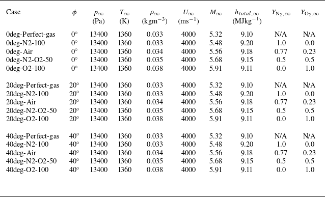

 kJmol−1


 Nx×Ny=512×128
 Nx×Ny=1024×256
 Nx×Ny=2048×512
 ΔXc
 Y=0mm


 Y

 0∘
 20∘
 40∘


 (X,Y)=(0mm,0mm)


 x
 x=100mm


 (X,Y)=(0mm,0mm)
 ϕ=20∘

 ϕ=0∘
 ϕ=20∘
 ϕ=40∘


 x
 ϕ=0∘
 ϕ=20∘
 ϕ=40∘

 x=100mm

 x=100

 YN
 YO

 x
 ϕ=0∘


 T
 TV

 Open access

