1. Introduction
Flow stratification – assumed to be of piecewise constant type in our work – is an intrinsic characteristic of geophysical water flows, particularly relevant to large-scale oceanic movements (cf. Gill Reference Gill1982; Marshall & Plumb Reference Marshall and Plumb2016; Constantin & Johnson Reference Constantin and Johnson2017; Vallis Reference Vallis2017). Strongly influenced by variations in temperature and salinity, density fluctuations occur frequently in the ocean and lead to a layered structure: fluid parcels of differing densities arrange themselves such that denser layers lie beneath lighter ones (cf. Kessler & McPhaden Reference Kessler and McPhaden1995; Fedorov & Brown Reference Fedorov, Brown and Steele2009; Cushman-Roisin & Beckers Reference Cushman-Roisin and Beckers2011; Constantin & Johnson Reference Constantin and Johnson2015). This vertical stratification results in the formation of interfaces between layers of distinct densities. Such a pronounced density stratification occurs within a region approximately 150 km wide on each side of the Equator, extending longitudinally over approximately 16 000 km in the Pacific Ocean. This stratification gives rise to a sharp thermocline (also referred to as a pycnocline), which acts as a waveguide for internal waves; cf. Fedorov & Brown (Reference Fedorov, Brown and Steele2009) and Constantin & Johnson (Reference Constantin and Johnson2015). At times, internal waves might have appreciable amplitudes: field data provide evidence for tide-generated internal waves with amplitudes in excess of 100 m, extending over 100 km; cf. Simmons et al. (Reference Simmons, Chang, Chang, Chao, Fringer, Jackson and Ko2011). Detailed, exact solutions depicting density stratified geophysical flows exhibiting internal waves were presented by Constantin (Reference Constantin2013, Reference Constantin2014).
From a practical side, the understanding of internal waves dynamics is important for mixing processes in oceans and submarine navigation, as well as for the need to quantify induced loads on submerged marine platforms.
Concerning the vertical stratification structure, it is widely accepted in oceanography (see Sutherland Reference Sutherland2010) that the ocean is effectively subdivided into layers according to the strength of its stratification. Accordingly we have: adjacent to the surface lies the mixed layer, named for the wind-driven stirring of surface waters; beneath it is the the strongly stratified thermocline; and below that is the weakly stratified deep layer composed of cold, dense water that constitutes the bulk of the ocean’s mass. Complementing this conceptual model, a series of laboratory experiments using a wind flume (Shintani & Umeyama Reference Shintani and Umeyama2001) simulated a three-layer density-stratified water body in which the middle layer (thermocline) was intentionally made thick, closely matching the thickness of the upper and lower layers. This deliberate configuration was designed to reflect stratification patterns observed in natural lakes, and to isolate the role of the thermocline. The study revealed that the thickness of the middle layer is a critical factor in shaping the system’s response to wind forcing, significantly influencing internal wave dynamics, energy transfer, and vertical mixing across the stratified column.
Minding the previous aspects concerning the type of layering in physically reasonable ocean flows, we consider in this study three-layer stratified water flows: the fluid domain is bounded above by the free surface and below by the (rigid) bottom boundary, and is split in three layers of constant, but different density. This type of stratification significantly complicates the analysis of an already highly intricate nonlinear problem. To alleviate these difficulties, we will rewrite the governing equations by means of a Hamiltonian (re)formulation. Such a reformulation highlights structural properties and has the advantage that it also reduces the numbers of variables in a way that results in significant simplifications. Note that the Hamiltonian formulation of the governing equations for two-dimensional gravity water flows was pioneered in Zakharov (Reference Zakharov1968) for irrotational flows, and was extended to rotational flows with constant vorticity in Constantin, Ivanov & Prodanov (Reference Constantin, Ivanov and Prodanov2007), Wahlén (Reference Wahlén2007, Reference Wahlén2008) and Compelli & Ivanov (Reference Compelli and Ivanov2017), and variable bottom in Craig et al. (Reference Craig, Guyenne and Kalisch2005), Compelli, Ivanov & Todorov (Reference Compelli, Ivanov and Todorov2018) and Compelli et al. (Reference Compelli, Ivanov, Martin and Todorov2019). The Hamiltonian formulation for two-dimensional irrotational two-layer gravity water flows with a free surface was developed in Craig, Guyenne & Kalisch (Reference Craig, Guyenne, Nicholls and Sulem2005), and the rotational counterpart with constant vorticity and constant density in each layer was obtained in Constantin, Ivanov & Martin (Reference Constantin, Ivanov and Martin2016) for the case of periodic flows. The validity of the Hamiltonian perspective in the presence of Coriolis forces in the equatorial
 $f$
-plane approximation, for zonal flows representing localised perturbations of an underlying pure current background state, was established in Constantin & Ivanov (Reference Constantin and Ivanov2019). We note that the power and relevance of Hamiltonian methods in the study of water flows is reinforced by the work of Craig, Guyenne & Sulem (Reference Craig, Guyenne and Sulem2015), where a relevant extension to three-dimensional flows is presented. Additionally, a mix of Hamiltonian methods and techniques related to the Dirichlet–Neumann (DN) operators is instrumental in the derivation of coupled nonlinear equations relating the interfaces and the traces of the velocity potentials on them, in various propagation regimes; cf. e.g. Craig et al. (Reference Craig, Guyenne, Nicholls and Sulem2005, Reference Craig, Guyenne and Sulem2011, Reference Craig, Guyenne and Sulem2015) and § 7.5 of this work.
The two- and three-layer dynamics have been studied actively, and various approximations have been employed, from Kakutani & Yamasaki (Reference Kakutani and Yamasaki1978) and Ovsyannikov (Reference Ovsyannikov1979) to the more recent Choi & Camassa (Reference Choi and Camassa1996, Reference Choi and Camassa1999), Camassa et al. (Reference Camassa, Falqui, Ortenzi, Pedroni and Ho2021), Cotter, Holm & Percival (Reference Cotter, Holm and Percival2010), Grimshaw et al. (Reference Grimshaw, Guo, Helfrich and Vlasenko2014), Ostrovsky & Helfrich (Reference Ostrovsky and Helfrich2019), de Melo Viríssimo & Milewski (Reference de Melo Viríssimo and Milewski2019) and Bona, Lannes & Saut (Reference Bona, Lannes and Saut2008). For recent results concerning exact solutions (in Lagrangian and Eulerian coordinates) describing water flows with stratification of discontinuous type, we refer the reader to Constantin (Reference Constantin2013, Reference Constantin2014), Matioc (Reference Matioc2012), Massel (Reference Massel2015), Escher et al. (Reference Escher, Knopf, Lienstromberg and Matioc2020) and Martin (Reference Martin2021).
Our aim is to present a Hamiltonian formulation and the full nonlinear equations of motion of two-dimensional stratified water flows consisting of three layers, each of which has constant density. We adopt a versatile framework for our investigations: the density in each layer can have any value, with the proviso that the stratification is of stable type. Moreover, the layers can have any thicknesses, without any constraints.
The paper is organised as follows. After introducing the model set-up and the governing equations in § 2, we show in § 3 that they can be rewritten as an infinite-dimensional Hamiltonian system. Furthermore, in § 3 we present the resulting full nonlinear equations of motion. They are expressed in terms of the so-called DN operators, which are introduced for the three-layer setting with a free surface. In § 4, the dispersion relation for the leading order of the wave amplitudes is derived for arbitrary wavelengths. Section 5 is devoted to the dispersion relation in the long-wave limit which is an intricate bi-cubic equation, whose solutions are all real numbers according to arguments presented in Benton (Reference Benton1954), Yih (Reference Yih1980) and Baines (Reference Baines1995). Exploiting a result by Prodanov (Reference Prodanov2022a ,Reference Prodanov b ), we give lower and upper bounds for these solutions. The limit to two layers is presented in § 6. Approximate solutions in certain regimes are also given. Section 7 is devoted to the three-layer rigid lid case. There again we present the full equations in terms of the DN operators, then by the expansion of the operators, we recover the dispersion relation of the system, and in addition we obtain the equations of the widely used nonlinear Boussinesq regime. Although the present study focuses on the three-layer model pertinent to oceanographic dynamics, we emphasise that the analytical framework and methodologies developed herein are broadly applicable to a wide range of scenarios involving interfacial internal waves across stratified fluid layers, extending well beyond the confines of saline ocean environments, and also to higher-order nonlinear approximations, if the quadratic ones are insufficient for the analysis.
2. Model set-up and governing equations
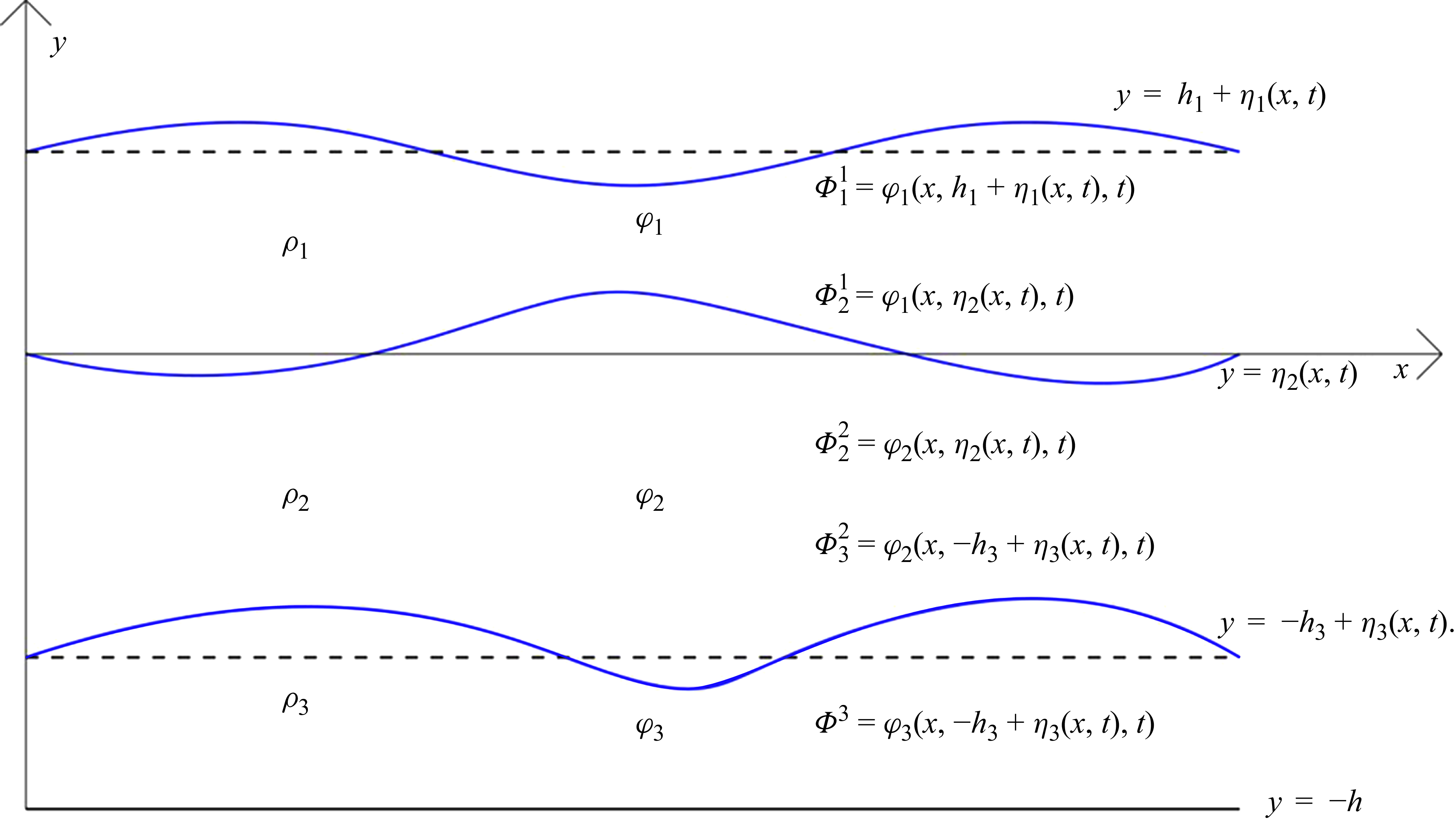
We assume that the fluid domain consists of a union of layers
 $\varOmega _i\ (i=1,2,3)$
depicted in figure 1 and defined as follows:
 \begin{align} \begin{split} &\varOmega _1:=\{(x,y,t): x\in \mathbb{R},t\in \mathbb{R},\eta _2(x,t)\lt y\lt h_1+\eta _1(x,t)\},\\[5pt] &\varOmega _2:=\{(x,y,t): x\in \mathbb{R},t\in \mathbb{R},-h_3+\eta _3(x,t)\lt y\lt \eta _2(x,t)\},\\[5pt] &\varOmega _3:=\{(x,y,t): x\in \mathbb{R},t\in \mathbb{R},-h\lt y\lt -h_3+\eta _3(x,t)\}, \end{split} \end{align}
where
 $h_1,h_3,h$
are positive constants such that
 $h\gt h_3$
, and
 $\eta _i(x,t)\in \mathcal{S}(\mathbb{R})$
for
 $i=1,2,3$
are Schwartz functions such that for all
 $i=1,2,3$
, the relations
 \begin{align} \int _{\mathbb{R}}\eta _i(x,t)\,{\rm d}x=0\quad \textrm {for}\, \, \textrm {all} \quad t \end{align}
hold. Relations (2.2) ensure that the average surface level of
 $\eta _1$
is at
 $y=h_1$
, the average surface level of
 $\eta _2$
is at
 $y=0$
, and the average surface level of
 $\eta _3$
is at
 $y=-h_3$
.
The system under study.

The density of the fluid is assumed to be piecewise constant at
 $\rho _i\ (i=1,2,3)$
in the layer
 $\varOmega _i$
for
 $i=1,2,3$
, and such that
 $\rho _1\lt \rho _2\lt \rho _3$
to account for the stable stratification. The same indicial notation will be used to denote the other physical quantities (e.g. the velocity field, the velocity potentials, the pressure). However, when we refer to the overall physical variable without specification of the layer, we will use the hat symbol placed on top of the variable. For example,
 $(\hat {u},\hat {v})$
will denote the velocity field that takes the value
 $(u_i,v_i)$
in the layer
 $\varOmega _i$
, for
 $i=1,2,3$
. Using
 $\hat {P}$
to denote the pressure, the equations of motion for an incompressible, inviscid flow are Euler’s equations
 \begin{align} \begin{array}{l@{\kern3pt}l} \hat {u}_t+\hat {u}\hat {u}_x+\hat {v}\hat {u}_y & =-\dfrac {1}{\hat {\rho }}\hat {P}_x,\\[7pt] \hat {v}_t+\hat {u}\hat {v}_x+\hat {v}\hat {v}_y &=-\dfrac {1}{\hat {\rho }}\hat {P}_y-g \end{array} \quad \mathrm{in} \quad \overline {\varOmega _1\cup \varOmega _2\cup \varOmega _3}, \end{align}
and the equation of mass conservation
 \begin{align} \hat {u}_x+\hat {u}_y=0 \quad \textrm {in} \quad \overline {\varOmega _1\cup \varOmega _2\cup \varOmega _3}. \end{align}
Equations (2.3) and (2.4) are complemented by appropriate boundary conditions. At the free surface, the dynamic boundary condition
 \begin{align} P_1=P_{\textit{atm}} \quad \textrm {on} \quad y=h_1+\eta _1(x,t) \end{align}
decouples the motion of the water from that of the air above, and at the same time ensures the balance of forces at the surface. Similarly, the balances of forces at the internal boundaries
 $y=\eta _2(x,t)$
and
 $y=-h_3+\eta _3(x,t)$
, respectively, are expressed by the conditions
 \begin{align} P_1=P_2 \quad \textrm {on} \quad y=\eta _2(x,t) \end{align}
and
 \begin{align} P_2=P_3 \quad \textrm {on} \quad y=-h_3+\eta _3(x,t). \end{align}
The kinematic boundary conditions, which refer to the flat bed
 $y=-h$
, the two interfaces
 $y=-h_3+\eta _3(x,t)$
and
 $y=\eta _2(x,t)$
, respectively, and to the free surface
 $y=h_1+\eta _1(x,t)$
, ensure that these surfaces are impermeable, thus no fluid particles cross them; they are stated as
 \begin{align} \begin{split} & v_1=\eta _{1,t}+u_1\eta _{1,x} \quad \textrm {on} \quad y=h_1+\eta _1(x,t),\\[3pt] & v_1=\eta _{2,t}+u_1\eta _{2,x} \quad \textrm {and}\quad v_2=\eta _{2,t}+u_2\eta _{2,x} \quad \textrm {on}\quad y=\eta _2(x,t),\\[3pt] &v_2=\eta _{3,t}+u_2\eta _{3,x} \quad \textrm {and}\quad v_3=\eta _{3,t}+u_3\eta _{3,x} \quad \textrm {on}\quad y={-h_3}+\eta _3(x,t),\\[3pt] &v_3=0 \quad \textrm {on}\quad y=-h. \end{split} \end{align}
Throughout the paper, we will assume that the fluid is rotation-free, i.e.
 \begin{align} \hat {u}_y(x,y,t)-\hat {v}_x(x,y,t)=0\quad\textrm {for}\, \, \textrm {all} \quad (x,y,t)\in \overline {\varOmega _1\cup \varOmega _2\cup \varOmega _3}. \end{align}
The irrotationality assumption (2.9) allows us to introduce now in each layer
 $\varOmega _i$
a velocity potential
 $\varphi _i\in C^1(\varOmega _i)$
that satisfies
 \begin{align} u_i=\varphi _{i,x} \quad \textrm {and} \quad v_i=\varphi _{i,y}\quad \textrm {for} \quad i=1,2,3. \end{align}
Remark 2.1. Note that due to (2.4), the velocity potentials
 $\varphi _i\ (i=1,2,3)$
are harmonic functions in
 $\varOmega _i,\ i=1,2,3.$
We will use, in the course of the paper, the subscripts
 ${s_1},{s_2},s_3$
in order to denote evaluations of various quantities on the surfaces
 $y=h_1+\eta _1(x,t)$
,
 $y=\eta _2(x,t)$
and
 $y=-h_3+\eta _3(x,t)$
, respectively. The kinematic boundary conditions can now be written as
 \begin{align} &\eta _{1,t}=(\varphi _{1,y})_{s_1}-\eta _{1,x}(\varphi _{1,x})_{s_1}, \\[-9pt] \nonumber \end{align}
 \begin{align} &\eta _{2,t}=(\varphi _{1,y})_{s_2}-\eta _{2,x}(\varphi _{1,x})_{s_2} =(\varphi _{2,y})_{s_2}-\eta _{2,x} (\varphi _{2,x} )_{s_2}, \\[-9pt] \nonumber \end{align}
 \begin{align} &\eta _{3,t}=(\varphi _{2,y})_{s_3}-\eta _{3,x} (\varphi _{2,x} )_{s_3}= (\varphi _{3,y})_{s_3}-\eta _{3,x}(\varphi _{3,x})_{s_3}. \\[9pt] \nonumber \end{align}
Moreover, the Euler equations can be recast as
 \begin{align} \begin{cases} \boldsymbol{\nabla }\left (\varphi _{1,t}+\dfrac {|\boldsymbol{\nabla }\varphi _1|^2}{2}+\dfrac {P_1}{\rho _1}+gy\right )=0 \quad \textrm {in} \quad \varOmega _1,\\[9pt] \boldsymbol{\nabla }\left (\varphi _{2,t}+\dfrac {|\boldsymbol{\nabla }\varphi _2|^2}{2}+\dfrac {P_2}{\rho _2}+gy\right )=0 \quad \textrm {in} \quad \varOmega _2,\\[9pt] \boldsymbol{\nabla }\left (\varphi _{3,t}+\dfrac {|\boldsymbol{\nabla }\varphi _3|^2}{2}+\dfrac {P_3}{\rho _3}+gy\right )=0 \quad \textrm {in} \quad \varOmega _3, \end{cases} \end{align}
where
 $\boldsymbol{\nabla}$
denotes the spatial gradient. Thus there are functions
 $t\mapsto f_i(t),\ i=1,2,3$
, such that
 \begin{align} \begin{cases} \varphi _{1,t}+\dfrac {|\boldsymbol{\nabla }\varphi _1|^2}{2}+\dfrac {P_1}{\rho _1}+gy=f_1(t) \quad \textrm {in} \quad \varOmega _1,\\[7pt] \varphi _{2,t}+\dfrac {|\boldsymbol{\nabla }\varphi _2|^2}{2}+\dfrac {P_2}{\rho _2}+gy=f_2(t) \quad \textrm {in} \quad \varOmega _2,\\[7pt] \varphi _{3,t}+\dfrac {|\boldsymbol{\nabla }\varphi _3|^2}{2}+\dfrac {P_3}{\rho _3}+gy=f_3(t) \quad \textrm {in} \quad \varOmega _3.\end{cases} \end{align}
Utilising the interface conditions (2.5), (2.6) and (2.7), and choosing convenient time-dependent functions
 $f_1,f_2,f_3$
in (2.15), we obtain the relations
 \begin{align} \begin{cases} \rho _1(\varphi _{1,t})_{s_1}+\rho _1 \dfrac {|\boldsymbol{\nabla }\varphi _1|^2_{s_1}}{2}+g\rho _1\eta _1=0,\\[7pt]\rho _1\left ((\varphi _{1,t})_{s_2}+\dfrac {|\boldsymbol{\nabla }\varphi _1|^2_{s_2}}{2}+g\eta _2 \right )= \rho _2\left ((\varphi _{2,t})_{s_2}+\dfrac {|\boldsymbol{\nabla }\varphi _2|^2_{s_2}}{2}+g\eta _2 \right )\!,\\[7pt]\rho _2\left ((\varphi _{2,t})_{s_3}+\dfrac {|\boldsymbol{\nabla }\varphi _2|^2_{s_3}}{2}+g\eta _3 \right )= \rho _3\left ((\varphi _{3,t})_{s_3}+\dfrac {|\boldsymbol{\nabla }\varphi _3|^2_{s_3}}{2}+g\eta _3 \right )\!. \end{cases} \end{align}
One of the main tenets of the Hamiltonian formulation refers to the possibility of reducing the number of the dynamical variables. This feature emerges, using the ansatz by Benjamin & Bridges (Reference Benjamin and Bridges1997a ,Reference Benjamin and Bridges b ) (utilised also by Craig, Guyenne & Sulem Reference Craig, Guyenne and Sulem2012). Let us define
 \begin{align} \begin{split} &\varPhi ^1_1:=\varphi _1(x,h_1+\eta _1(x,t),t)=(\varphi _1)_{s_1},\quad \varPhi ^1_2:=\varphi _1(x,\eta _2(x,t),t)=(\varphi _1)_{s_2},\\[4pt]&\varPhi ^2_2:=\varphi _2(x,\eta _2(x,t),t)=(\varphi _2)_{s_2},\quad \varPhi ^2_3:=\varphi _2(x,-h_3+\eta _3(x,t),t)=(\varphi _2)_{s_3},\\[4pt]&\varPhi ^3:=\varphi _3(x,-h_3+\eta _3(x,t),t)=(\varphi _3)_{s_3},\\[4pt]&\xi _1:=\rho _1\varPhi ^1_1,\quad \xi _2:=\rho _2\varPhi ^2_2-\rho _1\varPhi ^1_2,\quad \xi _3:=\rho _3\varPhi ^3-\rho _2\varPhi ^2_3. \end{split} \end{align}
In what follows, it will be shown that the five traces
 $\varPhi ^i_{\!j}$
can be expressed by the three Hamiltonian ‘momenta’
 $\xi _i$
only. The
 $\eta _i$
variables will play the role of Hamiltonian ‘coordinates’. This approach reduces not only the number of variables, but also the dimensionality of the problem, because instead of working in the bulk of the fluid (in the two-dimensional spatial domain), one can work only with variables defined on the surfaces and the interfaces, i.e. in one spatial dimension. We note that definition (2.17) arises naturally from the Legendre transform based on the Lagrangian; cf. formula (2.15) in Craig et al. (Reference Craig, Guyenne and Sulem2012).
Utilising the notation in (2.17), we obtain from (2.16) that
 $\xi _i$
satisfy the evolution equations
 \begin{align} \xi _{1,t} -\rho _1\eta _{1,t}(\varphi _{1,y})_{s_1}+\frac {\rho _1}{2}|\boldsymbol{\nabla }\varphi _1|^2_{s_1}+g\rho _1\eta _1 =0, \\[-28pt] \nonumber \end{align}
 \begin{align} \begin{split} \xi _{2,t}+\eta _{2,t}[\rho _1(\varphi _{1,y})_{s_2}-\rho _2(\varphi _{2,y})_{s_2}]+ \rho _2\frac {|\boldsymbol{\nabla }\varphi _2|^2_{s_2}}{2}-\rho _1\frac {|\boldsymbol{\nabla }\varphi _1|^2_{s_2}}{2} +(\rho _2-\rho _1)g\eta _2=0, \end{split} \\[-28pt] \nonumber \end{align}
 \begin{align} \begin{split} \xi _{3,t}+\eta _{3,t}[\rho _2(\varphi _{2,y})_{s_3}-\rho _3(\varphi _{3,y})_{s_3}]+ \rho _3\frac {|\boldsymbol{\nabla }\varphi _3|^2_{s_3}}{2}-\rho _2\frac {|\boldsymbol{\nabla }\varphi _2|^2_{s_3}}{2} +(\rho _3-\rho _2)g\eta _3=0. \end{split} \\[2pt] \nonumber \end{align}
3. The Hamiltonian formulation of the governing equations and the DN operators
In order to alleviate the difficulties brought about by the rich structure of the nonlinear water wave problem, a reformulation of the latter is needed. This is the Hamiltonian formulation that provides a choice of new dependent and independent variables in which the equations take their simplest form.
3.1. Hamiltonian form of the equations: equations for the moving surfaces
This subsection is devoted to a reformulation of the governing equations and of the boundary conditions (2.3)–(2.8) by collapsing the dynamical variables into a one-dimensional representation. More precisely, we will rewrite (2.3)–(2.8) as a Hamiltonian system of partial differential equations of the form (cf. Olver Reference Olver1993)
 \begin{align} \partial _t\mathfrak{m}=J\frac {\delta H}{\delta \mathfrak{m}}, \end{align}
where
 $t\mapsto \mathfrak{m}(t)$
denotes a path in a Hilbert space
 $\mathcal{H}$
equipped with an inner product
 $({\cdot },{\cdot })$
, and the associated Hamiltonian functional
 $H:\mathcal{D}\subset \mathcal{H}\rightarrow \mathbb{R}$
is defined on a dense subspace
 $\mathcal{D}$
of
 $\mathcal{H}$
. In our considerations
 $\mathfrak{m}=(\eta _1,\eta _2,\eta _3,\xi _1,\xi _2,\xi _3)^{\rm T}$
, the Hilbert space is an appropriate Cartesian product of spaces of square-integrable functions and
 $\mathcal{D}=\mathcal{S}(\mathbb{R})\times \mathcal{S}(\mathbb{R})\times \mathcal{S}(\mathbb{R})\times \mathcal{S}(\mathbb{R})\times \mathcal{S}(\mathbb{R})\times \mathcal{S}(\mathbb{R})$
, where
 $\mathcal{S}(\mathbb{R})$
is the subspace of Schwartz functions in the variable
 $x$
. Moreover,
 $J=\begin{pmatrix}0 & I_3\\-I_3 &0 \end{pmatrix}$
(where
 $I_3$
is the
 $3\times 3$
identity matrix) defines a Poisson bracket for functionals by the formula
 \begin{align} \{F_1,F_2\}=\left (\frac {\delta F_1}{\delta \mathfrak{m}},J\frac {\delta F_2}{\delta \mathfrak{m}}\right )\!. \end{align}
We also denote by
 ${\delta H}/{\delta \mathfrak{m}}$
the variational derivative of
 $H$
at
 $\mathfrak{m}\in \mathcal{D}$
through the formula
 \begin{align} \lim _{\varepsilon \to 0}\frac {H(\mathfrak{m}+\varepsilon \mathfrak{m}_0)-H(\mathfrak{m})}{\varepsilon }=\left (\mathfrak{m}_0,\frac {\delta H}{\delta \mathfrak{m}}\right )\quad \textrm {for} \quad \mathfrak{m}_0\in \mathcal{D}, \end{align}
where
 $({\cdot },{\cdot })$
is the inner product in the Hilbert space
 $L^2(\mathbb{R})\times L^2(\mathbb{R})\times L^2(\mathbb{R})\times L^2(\mathbb{R})\times L^2(\mathbb{R})\times L^2(\mathbb{R})$
.
3.2. The Hamiltonian functional
The natural candidate for the Hamiltonian functional is the total energy of the flow given as
 $E_K+E_P$
, where
 $E_K$
stands for the kinetic energy, and
 $E_P$
denotes the potential energy. In terms of the quantities of the flow, the kinetic energy is written as
 \begin{align} E_K=\iint_{\varOmega _1\cup \varOmega _2\cup \varOmega _3}\hat {\rho }\!\left (\frac {\hat {u}^2+\hat {v}^2}{2}\right ) {\rm d}y\,{\rm d}x, \end{align}
which, due to stratification and (2.10), can be detailed as
 \begin{align} E_K & = \int _{\mathbb{R}}\int _{-h}^{-h_3+\eta _3(x,t)}\rho _3\! \left (\frac {u_3^2+v_3^2}{2}\right ){\rm d}y\, {\rm d}x +\int _{\mathbb{R}}\int _{-h_3+\eta _3(x,t)}^{\eta _2(x,t)}\rho _2\! \left (\frac {u_2^2+v_2^2}{2}\right ){\rm d}y\, {\rm d}x \nonumber\\& \quad +\int _{\mathbb{R}}\int _{\eta _2(x,t)}^{h_1+\eta _1(x,t)}\rho _1\! \left (\frac {u_1^2+v_1^2}{2}\right ){\rm d}y\, {\rm d}x \nonumber\\\quad & = \frac {\rho _3}{2}\int _{\mathbb{R}}\int _{-h}^{-h_3+\eta _3(x,t)}|\boldsymbol{\nabla }\varphi _3|^2\,{\rm d}y\, {\rm d}x+ \frac {\rho _2}{2}\int _{\mathbb{R}}\int _{-h_3+\eta _3(x,t)}^{\eta _2(x,t)}|\boldsymbol{\nabla }\varphi _2|^2\,{\rm d}y\, {\rm d}x \nonumber\\& \quad +\frac {\rho _1}{2}\int _{\mathbb{R}}\int _{\eta _2(x,t)}^{h_1+\eta _1(x,t)}|\boldsymbol{\nabla }\varphi _1|^2\,{\rm d}y\, {\rm d}x. \end{align}
In defining the potential energy, we act on the realisation that not all the latter energy can be converted into kinetic energy. However, the difference in the potential energy between the perturbed wave state and the pure background state is available for this conversion. Hence we have
 \begin{align} E_P & = g\rho _3\int _{\mathbb{R}}\left (\int _{-h}^{-h_3+\eta _3}y\,{\rm d}y-\int _{-h}^{-h_3}y\,{\rm d}y\right )+g\rho _2\int _{\mathbb{R}}\left (\int _{-h_3+\eta _3}^{\eta _2}y\,{\rm d}y-\int _{-h_3}^0y\,{\rm d}y\right )\nonumber\\& \quad + g\rho _1\int _{\mathbb{R}}\left (\int _{\eta _2}^{h_1+\eta _1}y\,{\rm d}y-\int _0^{h_1}y\,{\rm d}y\right )\nonumber\\& = \frac {g\rho _1}{2}\int _{\mathbb{R}}\eta _1^2\,{\rm d}x+\frac {g(\rho _2-\rho _1)}{2}\int _{\mathbb{R}}\eta _2^2\,{\rm d}x + \frac {g(\rho _3-\rho _2)}{2}\int _{\mathbb{R}}\eta _3^2\,{\rm d}x. \end{align}
We note that the above choice for the potential energy allows us to avoid any non-physical constant terms in the energy density and hence infinite energy. More specifically, the potential energy functional (3.6) is not convergent if the potential energy of the pure current background state is not subtracted.
3.3. Computations of variations of
 $H$

We first list a few useful formulas for computing the variations of
 $H$
.
Remark 3.1.
-
(i) If
$F(x)=\int _{g_1(x)}^{g_2(x)}f(y)\,{\rm d}y$
for given real functions of one variable
$x\mapsto f(x)$
,
$x\mapsto g_1(x)$
and
$x\mapsto g_2(x)$
, then(3.7)
\begin{align} (\delta F)(x)=\int _{g_1(x)}^{g_2(x)}(\delta f)(y)\,{\rm d}y+f(g_2(x))(\delta g_2)(x)-f(g_1(x))(\delta g_1)(x). \end{align}
-
(ii) For given functions
$(x,y)\mapsto F(x,y)$
,
$x\mapsto f_i(x)\ (i=1,2)$
, we have(3.8)
\begin{align} \begin{split} \frac {\partial }{\partial x}\left (\int _{f_1(x)}^{f_2(x)}F(x,y)\,{\rm d}y\right )=&\int _{f_1(x)}^{f_2(x)}F_x(x,y)\,{\rm d}y\\ & {}+F(x,f_2(x))\,f_2'(x)-F(x,f_1(x))\,f_1'(x). \end{split} \end{align}
-
(iii) If
$\theta _1$
and
$\theta _2$
are harmonic functions satisfying
$\boldsymbol{\nabla }\boldsymbol{\cdot }(\theta _1\,\boldsymbol{\nabla }\theta _2)=(\boldsymbol{\nabla }\theta _1)\boldsymbol{\cdot }(\boldsymbol{\nabla }\theta _2)$
, then for harmonic variations
$\delta \varphi _i$
of
$\varphi _i$
, it holds that(3.9)since
\begin{align} \delta \big ((\boldsymbol{\nabla }\varphi _i)\boldsymbol{\cdot }(\boldsymbol{\nabla }\varphi _i)\big )=2\,\boldsymbol{\nabla }\boldsymbol{\cdot }(\delta \varphi _i\,\boldsymbol{\nabla }\varphi _i), \end{align}
$|\boldsymbol{\nabla }\varphi _i|^2=\boldsymbol{\nabla }\boldsymbol{\cdot }(\varphi _i\, \boldsymbol{\nabla }\varphi _i)$
for
$i=1,2,3$
.


Remark 3.2. Regarding variations of the traces on the interfaces of the velocity potentials, the following formulas are true.
-
(i) On the free surface
$y=h_1+\eta _1(x,t)$
, we have(3.10)
\begin{align} & (\delta\varPhi _1^1)(x,t)\nonumber \\ &\, =\lim _{\varepsilon \to 0}\frac {(\varphi _1+\varepsilon\, \delta \varphi _1)\big (x,h_1+\eta _1(x,t)+\varepsilon (\delta \eta _1)(x,t),t\big )-\varphi _1(x,h_1+\eta (x,t),t)}{\varepsilon } \nonumber \\ &\,=(\varphi _{1,y})_{s_1}\,\delta \eta _1+(\delta \varphi _1)_{s_1}. \end{align}
-
(ii) Analogously, on the interface
$y=\eta _2(x,t)$
, we have(3.11)
\begin{align} \delta \varPhi ^1_2=(\varphi _{1,y})_{s_2}\,\delta \eta _2+(\delta \varphi _1)_{s_2}\quad \textrm {and}\quad \delta \varPhi _2^2=(\varphi _{2,y})_{s_2}\,\delta \eta _2+(\delta \varphi _2)_{s_2}. \end{align}
-
(iii) Finally, on the interface
$y=-h_3+\eta _3(x,t)$
, we have(3.12)
\begin{align} \delta \varPhi ^2_3=(\varphi _{2,y})_{s_3}\,\delta \eta _3+(\delta \varphi _2)_{s_3}\quad \textrm {and}\quad (\varphi _{3,y})_{s_3}\,\delta \eta _3+(\delta \varphi _3)_{s_3}. \end{align}


We proceed now to compute the variations of the terms that make up the kinetic energy
 $E_K$
from (3.5). Utilising the divergence theorem (Evans Reference Evans2010), and (3.12) as well as (3.7), (3.8) and (3.9), we obtain
 \begin{align} \delta \left (\int _{\mathbb{R}}\int _{-h}^{-h_3+\eta _3}|\boldsymbol{\nabla }\varphi _3|^2\,{\rm d}y\,{\rm d}x\right )={}&2 \int _{\mathbb{R}}(\varphi _{3,y}-\eta _{3,x}\varphi _{3,x})_{s_3} \big (\delta \varPhi ^3-(\delta \eta _3)(\varphi _{3,y})_{s_3}\big ){\rm d}x \nonumber\\ & \quad +\int _{\mathbb{R}}|\boldsymbol{\nabla }\varphi _3|^2_{s_3}\delta \eta _3\, {\rm d}x. \end{align}
Analogously, by the same token we have
 \begin{align} \delta \left (\int _{\mathbb{R}}\int _{-h_3+\eta _3}^{\eta _2}|\boldsymbol{\nabla }\varphi _2|^2\,{\rm d}y\,{\rm d}x\right ) & = 2 \int _{\mathbb{R}} (\varphi _{2,y}-\eta _{2,x}\varphi _{2,x})_{s_2} \big (\delta \varPhi ^2_2-(\delta \eta _2)(\varphi _{2,y})_{s_2}\big ) {\rm d}x \nonumber\\& \quad -2 \int _{\mathbb{R}} (\varphi _{2,y}-\eta _{3,x}\varphi _{2,x})_{s_3} \big (\delta \varPhi ^2_3-(\delta \eta _3)(\varphi _{2,y})_{s_3}\big ) {\rm d}x \nonumber\\& \quad +\int _{\mathbb{R}}|\boldsymbol{\nabla }\varphi _2|^2_{s_2}\delta \eta _2\,{\rm d}x -\int _{\mathbb{R}}|\boldsymbol{\nabla }\varphi _2|^2_{s_3}\delta \eta _3\,{\rm d}x \end{align}
and
 \begin{align} \delta \left (\int _{\mathbb{R}}\int _{\eta _2}^{h_1+\eta _1}|\boldsymbol{\nabla }\varphi _1|^2\,{\rm d}y\,{\rm d}x\right ) & = 2 \int _{\mathbb{R}} (\varphi _{1,y}-\eta _{1,x}\varphi _{1,x})_{s_1} \big (\delta \varPhi ^1_1-(\delta \eta _1)(\varphi _{1,y})_{s_1}\big ) {\rm d}x \nonumber\\& \quad-2 \int _{\mathbb{R}} (\varphi _{1,y}-\eta _{2,x}\varphi _{1,x})_{s_2} \big (\delta \varPhi ^1_2-(\delta \eta _2)(\varphi _{1,y})_{s_2}\big ) {\rm d}x \nonumber\\& \quad +\int _{\mathbb{R}}|\boldsymbol{\nabla }\varphi _1|^2_{s_1}\delta \eta _1\,{\rm d}x -\int _{\mathbb{R}}|\boldsymbol{\nabla }\varphi _1|^2_{s_2}\delta \eta _2\,{\rm d}x. \end{align}
Collecting together the variations of
 $H$
(from (3.13)–(3.15) and (3.6)) with respect to
 $\eta _1$
,
 $\eta _2$
and
 $\eta _3$
, respectively, we find that
 \begin{align} \frac {\delta H}{\delta \eta _1}&=-\rho _1\,\eta _{1,t}(\varphi _{1,y})_{s_1}+\frac {\rho _1}{2}|\boldsymbol{\nabla }\varphi _1|^2_{s_1}+g\rho _1\eta _1 \nonumber\\&=-\rho _1\,\eta _{1,t}(\varphi _{1,y})_{s_1}-\rho _1(\varphi _{1,t})_{s_1} \nonumber\\&=-\frac {{\rm d}}{{\rm d}t}\left (\rho _1\,\varphi _1(x,h_1+\eta _1(x,t),t)\right ) \nonumber\\&=-\xi _{1,t}, \\[-28pt] \nonumber \end{align}
 \begin{align} \frac {\delta H}{\delta \eta _2}&=\rho _1\,\eta _{2,t}(\varphi _{1,y})_{s_2}-\frac {\rho _1}{2}|\boldsymbol{\nabla }\varphi _1|^2_{s_2}-\rho _2\,\eta _{2,t}(\varphi _{2,y})_{s_2}+\frac {\rho _2}{2}|\boldsymbol{\nabla }\varphi _2|^2_{s_2}+(\rho _2-\rho _1)g\eta _2 \nonumber \\&=-\rho _2\left ((\varphi _{2,t})_{s_2}+\eta _{2,t}(\varphi _{2,y})_{s_2}\right )+\rho _1\left ((\varphi _{1,t})_{s_2}+\eta _{2,t}(\varphi _{1,y})_{s_2}\right ) \nonumber\\&=-\frac {{\rm d}}{{\rm d}t}\left (\rho _2\,\varphi _2(x,\eta _2(x,t),t)\right )+\frac {{\rm d}}{{\rm d}t}\left (\rho _1\,\varphi _1(x,\eta _2(x,t),t)\right ) \nonumber\\&=-\xi _{2,t} \\[2pt] \nonumber \end{align}
and
 \begin{align} \frac {\delta H}{\delta \eta _3}&=\rho _2\,\eta _{3,t}(\varphi _{2,y})_{s_3}-\frac {\rho _2}{2}|\boldsymbol{\nabla }\varphi _2|^2_{s_3}-\rho _3\,\eta _{3,t}(\varphi _{3,y})_{s_3}+\frac {\rho _3}{2}|\boldsymbol{\nabla }\varphi _3|^2_{s_3}+(\rho _3-\rho _2)g\eta _3 \nonumber \\&=-\rho _3\left ((\varphi _{3,t})_{s_3}+\eta _{3,t}(\varphi _{3,y})_{s_3}\right )+\rho _2\left ((\varphi _{2,t})_{s_3}+\eta _{3,t}(\varphi _{2,y})_{s_3}\right ) \nonumber \\&=-\frac {{\rm d}}{{\rm d}t}\left (\rho _3\,\varphi _3(x,-h_3+\eta _3(x,t),t)\right )+\frac {{\rm d}}{{\rm d}t}\left (\rho _2\,\varphi _2(x,-h_3+\eta _3(x,t),t)\right )\nonumber \\&=-\xi _{3,t}. \end{align}
Moreover, glancing at (2.17) and utilising (3.13)–(3.15), we infer that
 \begin{align} \frac {\delta H}{\delta \xi _1}=\eta _{1,t},\quad \frac {\delta H}{\delta \xi _2}=\eta _{2,t},\quad \frac {\delta H}{\delta \xi _3}=\eta _{3,t}. \end{align}
We summarise the conclusions regarding the variations of
 $H$
computed in (3.16), (3.17), (3.18) and (3.19) in the following theorem.
Theorem 3.3. The governing equations and boundary conditions (2.3)–(2.8) possess the Hamiltonian formulation
 \begin{align} \begin{cases} \dfrac {\delta H}{\delta \eta _1}=-\xi _{1,t},\quad \dfrac {\delta H}{\delta \xi _1}=\eta _{1,t},\\[9pt] \dfrac {\delta H}{\delta \eta _2}=-\xi _{2,t},\quad \dfrac {\delta H}{\delta \xi _2}=\eta _{2,t},\\[9pt] \dfrac {\delta H}{\delta \eta _3}=-\xi _{3,t},\quad \dfrac {\delta H}{\delta \xi _3}=\eta _{3,t}. \end{cases} \end{align}
Remark 3.4. The (equivalent) Hamiltonian (re)formulation of the water wave problem not only reduces the number of the dynamical variables, but (together with the DN machinery) also offers the possibility to derive (simpler) nonlinear model equations directly from the full nonlinear water waves equations in multi-layer flows with a free surface. As a result, the coefficients in these equations (and also their solutions) depend explicitly on physical parameters on the multi-layer system; cf. Craig et al. (Reference Craig, Guyenne, Nicholls and Sulem2005, Reference Craig, Guyenne and Sulem2012) and Constantin & Ivanov (Reference Constantin and Ivanov2019). More precisely, from a single overarching principle – the Hamiltonian formulation – one can derive model equations pertaining to various physical regimes by simply defining suitable scaling regimes in terms of certain ratios such as amplitude/layer depth and/or amplitude/wavelength; cf. e.g. Craig et al. (Reference Craig, Guyenne, Nicholls and Sulem2005, Reference Craig, Guyenne and Sulem2012) and Constantin & Ivanov (Reference Constantin and Ivanov2019). This is in stark contrast to the usual case-by-case analysis (Whitham Reference Whitham1999). Furthermore, the Hamiltonian perspective is very suited to perturbation analysis since it guarantees that if appropriate symmetries are preserved in the approximation process, then conservation properties of the exact system are retained in its approximations.
3.4. The DN operators
The DN operator corresponding to the uppermost layer is defined as
 \begin{align} \begin{pmatrix}G_{11} & G_{12}\\ G_{21} & G_{22}\end{pmatrix}\begin{pmatrix}(\varphi _{1})_{s_2}\\ (\varphi _{1})_{s_1}\end{pmatrix}= \begin{pmatrix} -\sqrt {1+\eta _{2,x}^2}\left (\dfrac{\partial \varphi _1}{\partial \boldsymbol{n}_2} \right )_{s_2} \\[6pt] \sqrt {1+\eta _{1,x}^2}\left (\dfrac{\partial \varphi _1}{\partial \boldsymbol{n}_1} \right )_{s_1} \end{pmatrix} \!, \end{align}
where
 $\boldsymbol{n}_2={(-\eta _{2,x},1)}/{\sqrt {1+\eta _{2,x}^2}}$
and
 $\boldsymbol{n}_1={(-\eta _{1,x},1)}/{\sqrt {1+\eta _{1,x}^2}}$
are the unit normal vectors to the upper interface
 $y=\eta _2(x,t)$
and to the top surface
 $y=-h_1+\eta _1(x,t)$
, respectively. The DN operator corresponding to the middle layer is
 \begin{align} \begin{pmatrix}\varGamma _{11} & \varGamma _{12}\\ \varGamma _{21} &\varGamma _{22}\end{pmatrix}\begin{pmatrix}(\varphi _2)_{s_2}\\ (\varphi _2)_{s_3}\end{pmatrix}= \begin{pmatrix} \sqrt {1+\eta _{2,x}^2}\left (\dfrac{\partial \varphi _2}{\partial \boldsymbol{n}_2} \right )_{s_2} \\[6pt] -\sqrt {1+\eta _{3,x}^2}\left (\dfrac{\partial \varphi _2}{\partial \boldsymbol{n}_3} \right )_{s_3} \end{pmatrix} \!, \end{align}
where
 $\boldsymbol{n}_3={(-\eta _{3,x},1)}/{\sqrt {1+\eta _{3,x}^2}}$
denotes the outward pointing unit normal vector corresponding to the lower interface
 $y=-h_3+\eta _3(x,t)$
. Moreover, the DN operator corresponding to the bottom layer is
 \begin{align} G(\eta _3)(\varphi _3)_{s_3}=\sqrt {1+\eta _{3,x}^2}\left ({\partial \varphi _3}/{\partial \boldsymbol{n}_3}\right )_{s_3}=(\boldsymbol{\nabla }\varphi _3)_{s_3}\boldsymbol{\cdot }(-\eta _{3,x},1). \end{align}
These DN operators for each domain
 $\varOmega_1,\varOmega_2,\varOmega_3$
could be obtained recursively in the form of asymptotic series in
 $\eta _1, \eta _2, \eta_3$
following the technique described in the Appendix of Craig et al. (Reference Craig, Guyenne, Nicholls and Sulem2005); see also Appendix A of Ivanov, Martin & Todorov (Reference Ivanov, Martin and Todorov2022).
Appealing to the divergence theorem (Evans Reference Evans2010), the kinetic energy of the system (3.5) can be rewritten as
 \begin{align} {\rm E}_K & = \frac {\rho _1}{2}\int (\varphi _1)_{s_1}\left (\boldsymbol{\nabla }\varphi _1\right )_{s_1}\boldsymbol{\cdot }(-\eta _{1,x},1)\,{\rm d}x -\frac {\rho _1}{2}\int (\varphi _1)_{s_2}\left (\boldsymbol{\nabla }\varphi _1\right )_{s_2}\boldsymbol{\cdot }(-\eta _{2,x},1)\,{\rm d}x \nonumber\\& \quad + \frac {\rho _2}{2}\int (\varphi _2)_{s_2}\left (\boldsymbol{\nabla }\varphi _2\right )_{s_2}\boldsymbol{\cdot }(-\eta _{2,x},1)\,{\rm d}x -\frac {\rho _2}{2}\int (\varphi _2)_{s_3}\left (\boldsymbol{\nabla }\varphi _2\right )_{s_3}\boldsymbol{\cdot }(-\eta _{3,x},1)\,{\rm d}x \nonumber\\& \quad +\frac {\rho _3}{2}\int (\varphi _3)_{s_3}\left (\boldsymbol{\nabla }\varphi _3\right )_{s_3}\boldsymbol{\cdot }(-\eta _{3,x},1)\,{\rm d}x. \end{align}
With the help of the DN operators, the kinetic energy can be written as
 \begin{align} {\rm E}_K & = \frac {\rho _1}{2}\int (\varphi _1)_{s_1}\left [G_{21}(\varphi _1)_{s_2}+G_{22}(\varphi _1)_{s_1}\right ]\,{\rm d}x \nonumber\\& \quad +\frac {\rho _1}{2}\int (\varphi _1)_{s_2}\left [G_{11}(\varphi _1)_{s_2}+G_{12}(\varphi _1)_{s_1}\right ]\,{\rm d}x \nonumber\\& \quad +\frac {\rho _2}{2}\int (\varphi _2)_{s_2}\left [\varGamma _{11}(\varphi _2)_{s_2} +\varGamma _{12}(\varphi _2)_{s_3}\right ]\,{\rm d}x \nonumber\\& \quad +\frac {\rho _2}{2}\int (\varphi _2)_{s_3}\left [\varGamma _{21}(\varphi _2)_{s_2} +\varGamma _{22}(\varphi _2)_{s_3}\right ]\,{\rm d}x \nonumber\\& \quad +\frac {\rho _3}{2}\int (\varphi _3)_{s_3} G(\eta _3)(\varphi _3)_{s_3}\,{\rm d}x. \end{align}
Attempting to simplify (3.25) we note first that from the kinematic condition at the upper interface
 $y=\eta _2(x,t)$
, we have
 \begin{align} \eta _{2,t}=(\boldsymbol{\nabla }\varphi _2)_{s_2}\boldsymbol{\cdot }(\eta _{2,x},-1)=(\boldsymbol{\nabla }\varphi _1)_{s_2}\boldsymbol{\cdot }(\eta _{2,x},-1), \end{align}
which, in terms of the DN operators, becomes
 \begin{align} \eta _{2,t}=-(\varGamma _{11}(\varphi _2)_{s_2}+\varGamma _{12}(\varphi _2)_{s_3})=G_{11}(\varphi _1)_{s_2}+G_{12}(\varphi _1)_{s_1}. \end{align}
Moreover,
 \begin{align} \eta _{3,t}=(\varphi _{2,y}-\varphi _{2,x}\eta _{3,x})_{s_3}=(\varphi _{3,y}-\varphi _{3,x}\eta _{3,x})_{s_3}, \end{align}
which implies
 \begin{align} \eta _{3,t}=G(\eta _3)(\varphi _3)_{s_3}=- \big[\varGamma _{21}(\varphi _2)_{s_2} +\varGamma _{22}(\varphi _2)_{s_3}\big]. \end{align}
Recalling that
 \begin{align} \xi _1=\rho _1(\varphi _1)_{s_1},\quad\xi _2=\rho _2 (\varphi _2)_{s_2}-\rho _1 (\varphi _1)_{s_2},\quad\xi _3=\rho _3 (\varphi _3)_{s_3}-\rho _2(\varphi _2)_{s_3}, \end{align}
and employing (3.27) and (3.29), we see that the kinetic energy can be simplified as
 \begin{align} \begin{split} {E}_{K}={}&\frac {1}{2}\int \xi _1\left [G_{21}(\varphi _1)_{s_2}+G_{22}(\varphi _1)_{s_1}\right ]\,{\rm d}x \\ &{}+\frac {1}{2}\int \xi _2\left [\varGamma _{11}(\varphi _2)_{s_2} +\varGamma _{12}(\varphi _2)_{s_3}\right ]\,{\rm d}x\\ &{}+\frac {1}{2}\int \xi _3\, G(\eta _3)(\varphi _3)_{s_3}\,{\rm d}x. \end{split} \end{align}
Moreover, from (3.27) and (3.29), we also obtain the system
 \begin{align} \xi _2 &=\rho _2 (\varphi _2)_{s_2}+\rho _1 G_{11}^{-1}[\varGamma _{11}(\varphi _2)_{s_2} +\varGamma _{12}(\varphi _2)_{s_3}+\rho _1^{-1}G_{12}\xi _1], \\[-9pt] \nonumber \end{align}
 \begin{align} \xi _3&=-\rho _2 (\varphi _2)_{s_3}-\rho _3\, G^{-1}(\eta _3)\,[\varGamma _{21}(\varphi _2)_{s_2} +\varGamma _{22}(\varphi _2)_{s_3}], \\[9pt] \nonumber \end{align}
which can be rearranged as
 \begin{align} \begin{split} (\rho _2+\rho _1 G_{11}^{-1}\varGamma _{11})(\varphi _2)_{s_2}+(\rho _1 G_{11}^{-1}\varGamma _{12})(\varphi _2)_{s_3} &=\xi _2-G_{11}^{-1}G_{12}\xi _1,\\ (-\rho _3\, G^{-1}(\eta _3)\,\varGamma _{21})(\varphi _2)_{s_2} -(\rho _2 +\rho _3\, G^{-1}(\eta _3)\,\varGamma _{22})(\varphi _2)_{s_3} &=\xi _3, \end{split} \end{align}
where the superscript
 $-1$
in the previous system (and in the subsequent equations) is used to refer to the inverse of the operator in question.
Taking into account the fact that (3.34) is a linear system of equations with operator-valued coefficients, we obtain
 \begin{align} \begin{split} &(\varphi _2)_{s_2}=\mathcal{D}^{-1}\big ( \rho _1 G \xi _3 + (\rho _2 G+\rho _3\varGamma _{22})\varGamma _{12}^{-1}(G_{11}\xi _2-G_{12}\xi _1) \big )\equiv \varPhi _2^2(\eta _i, \xi _i), \\ &(\varphi _2)_{s_3}=-(\mathcal{D}^*)^{-1}\big ( \rho _3(G_{11}\xi _2-G_{12}\xi _1) + (\rho _2 G_{11}+\rho _1\varGamma _{11})\varGamma _{21}^{-1} G \xi _3 \big ), \end{split} \end{align}
where
 $\mathcal{D}:= ( (\rho _2 G+\rho _3\varGamma _{22})\varGamma _{12}^{-1}(\rho _2 G_{11}+\rho _1\varGamma _{11})-\rho _1 \rho _3 \varGamma _{21} )$
, and the star
 $(*)$
notation denotes the operation of conjugation. (The conjugation is with respect to the standard real bilinear form
 $(f,g)=\int _{\mathbb{R}} f(x)\, g(x)\, {\rm d}x$
.) We used also the fact that
 $G_{\textit{ij}}=G^*_{\textit{ji}}$
and
 $\varGamma _{\textit{ij}}=\varGamma ^*_{\textit{ji}}$
; see e.g. Craig et al. (Reference Craig, Guyenne, Nicholls and Sulem2005). Moreover, from (3.30), we also have
 \begin{align} (\varphi _1)_{s_2} & =\frac {1}{\rho _1}\mathcal{D}^{-1}\big ( \rho _1 (\rho _2 G \xi _3 +\rho _3\varGamma _{21} \xi _2)- (\rho _2 G+\rho _3\varGamma _{22})\varGamma _{12}^{-1}(\rho _2 G_{12}\xi _1+\rho _1 \varGamma _{11}\xi _2) \big ) \nonumber \\ & \equiv \varPhi ^1_2(\eta _i, \xi _i), \nonumber \\(\varphi _3)_{s_3}& =-(\mathcal{D}^*)^{-1}\big ( \rho _2 G_{11}\xi _2-\rho _2 G_{12}\xi _1+\rho _1 \varGamma _{12}\xi _3 {-} (\rho _2 G_{11}+\rho _1\varGamma _{11})\varGamma _{21}^{-1} \varGamma _{22} \xi _3 \big ). \end{align}
The previous expressions of the surface values of the potentials together with (3.6) allow us to express the Hamiltonian as a functional of the quantities
 $\eta _i,\xi _i\ (i=1,2,3)$
, i.e. we have
 \begin{align} \begin{split} H={}&{{E}_{{K}}(\xi _i)}+V(\eta _i)\\ ={}&\frac {1}{2}\int \xi _1 A_{11} \xi _1 \,{\rm d}x + \frac {1}{2}\int \xi _2 A_{22} \xi _2 \,{\rm d}x+\frac {1}{2}\int \xi _3 A_{33} \xi _3 \,{\rm d}x \\ &{}+ \int \xi _1 A_{12} \xi _2 \, {\rm d}x + \int \xi _1 A_{13} \xi _3 \, {\rm d}x + \int \xi _2 A_{23} \xi _3 \, {\rm d}x \\ &{}+\frac {1}{2} \int \big ( g\rho _1 \eta _1^2 +g(\rho _2-\rho _1) \eta _2^2 + g(\rho _3-\rho _2) \eta _3^2\big ) \, {\rm d}x, \end{split} \end{align}
where the last integral is the potential energy
 $V$
, and the operators
 $A_{\textit{ij}}\ (i,j=1,2,3)$
, written in terms of the DN operators, are
 \begin{align} &A_{11}=\frac {1}{\rho _1}G_{22}- \frac {\rho _2}{\rho _1} G_{21}\mathcal{D}^{-1}(\rho _2 G +\rho _3 \varGamma _{22})\varGamma _{12}^{-1}G_{12} , \nonumber\\&A_{22}= \varGamma _{11} \mathcal{D}^{-1} (\rho _2 G + \rho _3 \varGamma _{22})\varGamma _{12}^{-1}G_{11}-\rho _3 G_{11} \mathcal{D}^{-1} \varGamma _{21}, \nonumber\\& A_{33}= \big ( \varGamma _{22} \varGamma _{12}^{-1}(\rho _2 G_{11}+\rho _1 \varGamma _{11}) -\rho _1 \varGamma _{21} \big )\mathcal{D}^{-1} G,\nonumber\\&A_{12}=\rho _3 G_{21} \mathcal{D}^{-1} \varGamma _{21} - \frac {1}{2} G_{21}\big ( \mathcal{D}^{-1}(\rho _2 G + \rho _3 \varGamma _{22})\varGamma _{12}^{-1}+ \varGamma _{21}^{-1} (\rho _2 G + \rho _3 \varGamma _{22}) (\mathcal{D}^*)^{-1} \big )\varGamma _{11},\nonumber\\&A_{13}=\frac {1}{2}\rho _2 G_{21} \big (\mathcal{D}^{-1}+(\mathcal{D}^*)^{-1}\big )G,\nonumber\\&A_{23}=\frac {1}{2}\big ( (\rho _1 \varGamma _{11}-\rho _2 G_{11}) \mathcal{D}^{-1} - \varGamma _{12} (\mathcal{D}^*)^{-1} (\rho _2 G_{11}+\rho _1 \varGamma _{11})\varGamma _{21}^{-1}\big ) G. \end{align}
The Hamiltonian equations can be represented, via the DN operators, with the help of the quantities
 $(\varphi _{1,x}(x,y,t))_{s_1}$
and
 $(\varphi _{1,y}(x,y,t))_{s_1}$
. From (3.37) and because the operators
 $A_{\textit{ij}}$
do not depend on
 $\xi _i$
, we obtain (in terms of the Hamiltonian variables) the evolution equation
 \begin{align} \eta _{1,t}=\frac {\delta H}{\delta \xi _1}=A_{11}\xi _1+A_{12}\xi _2+A_{13}\xi _3:=F_1(\eta _i,\xi _i). \end{align}
In addition, by (3.37) and (3.20),
 $(\varphi _{1,x}(x,y,t))_{s_1}$
and
 $(\varphi _{1,y}(x,y,t))_{s_1}$
satisfy the system
 \begin{align} \begin{split} &(\varphi _{1,x})_{s_1}+(\varphi _{1,y})_{s_1} \eta _{1,x}= \frac {1}{\rho _1}\xi _{1,x},\\ &(\varphi _{1,y})_{s_1}-(\varphi _{1,x})_{s_1}\eta _{1,x}=\eta _{1,t}=F_1(\eta _i,\xi _i). \end{split} \end{align}
Solving the system, we find
 \begin{align} \begin{split} & (\varphi _{1,x})_{s_1}= \frac {\xi _{1,x}-\rho _1\eta _{1,x} F_1}{\rho _1 \big(1+\eta _{1,x}^2 \big)} , \\&(\varphi _{1,y})_{s_1}= \frac {\eta _{1,x}\xi _{1,x}+\rho _1 F_1}{\rho _1 \big(1+\eta _{1,x}^2 \big)}, \end{split} \end{align}
which allow us to write (2.18) through the Hamiltonian variables. More precisely, we have
 \begin{align} \xi _{1,t} + \frac {\xi _{1,x}^2 -2\rho _1\eta _{1,x}\xi _{1,x}F_1- \rho _1^2F_1^2}{2\rho _1 \big(1+\eta _{1,x}^2 \big)} +g\rho _1\eta _1 =0. \end{align}
The counterpart equation for
 $\eta _1$
is of course (3.39),
 \begin{align} \eta _{1,t} = F_1(\xi _i,\eta _i). \end{align}
From (3.37), where the operators
 $A_{\textit{ij}}$
do not depend on
 $\xi _i$
, we have
 \begin{align} \eta _{2,t}=\frac {\delta H}{\delta \xi _2}= A_{12}^* \xi _1+A_{22}\xi _2+A_{23} \xi _3 =: F_2(\eta _i,\xi _i). \end{align}
Thus
 $F_2(\eta _i,\xi _i)$
is defined through the canonical variables. Next, from (3.35) we have
 $(\varphi _2)_{s_2}\equiv \varPhi _2^2(\eta _i, \xi _i)$
as a known quantity, defined through the canonical variables. Since
 \begin{align} \frac {{\rm d}}{{\rm d}x} \varPhi _2^2= (\varphi _{2,x} )_{s_2}+(\varphi _{2,y})_{s_2}\eta _{2,x}, \end{align}
and from (2.12)
 \begin{align} F_2=\eta _{2,t}=(\varphi _{2,y})_{s_2}-(\varphi _{2,x} )_{s_2}\eta _{2,x}, \end{align}
we have a system
 \begin{align} & (\varphi _{2,x} )_{s_2}+ \eta _{2,x}(\varphi _{2,y})_{s_2}= (\varPhi ^2_2 )_x, \\[-9pt] \nonumber \end{align}
 \begin{align} -&\eta _{2,x} (\varphi _{2,x} )_{s_2}+(\varphi _{2,y})_{s_2}=F_2, \\[9pt] \nonumber \end{align}
which gives
 \begin{align} (\varphi _{2,x} )_{s_2}&= \frac {(\varPhi ^2_2)_x-\eta _{2,x}F_2}{1+\eta _{2,x}^2 }, \\[-12pt] \nonumber \end{align}
 \begin{align} (\varphi _{2,y})_{s_2}&= \frac {\eta _{2,x}(\varPhi ^2_2)_x +F_2}{1+\eta _{2,x}^2 }, \\[9pt] \nonumber \end{align}
and similarly,
 \begin{align} (\varphi _{1,x})_{s_2}&= \frac {(\varPhi ^1_2)_x-\eta _{2,x}F_2}{1+\eta _{2,x}^2 }, \\[-12pt] \nonumber \end{align}
 \begin{align} (\varphi _{1,y})_{s_2}&= \frac {\eta _{2,x}(\varPhi ^1_2)_x +F_2}{1+\eta _{2,x}^2 }, \\[9pt] \nonumber \end{align}
where
 $\varPhi ^1_2$
is defined in (3.36). Therefore,
 $\xi _2$
satisfies the equation
 \begin{align} \xi _{2,t}+\frac {\rho _2 (\varPhi ^2_{2,x} )^2-\rho _1 (\varPhi _{2,x}^1 )^2-2F_2\xi _{2,x}\eta _{2,x}+(\rho _1-\rho _2)F_2^2 }{2 \big(1+\eta _{2,x}^2 \big)}+(\rho _2-\rho _1)g \eta _2 =0. \end{align}
Similarly, for the last pair of equations, we obtain
 \begin{align} \eta _{3,t}=\frac {\delta H}{\delta \xi _3}=A_{13}^{*}\xi _1 +A_{23}^{*}\xi _2+A_{33}\xi _3:=F_3(\eta _i,\xi _i) \end{align}
and
 \begin{align} \xi _{3,t}+\frac {\rho _3 (\varPhi ^3_{x} )^2-\rho _2 (\varPhi _{3,x}^2 )^2-2F_3\xi _{3,x}\eta _{3,x}+(\rho _2-\rho _3)F_3^2 }{2\big(1+\eta _{3,x}^2 \big)}+(\rho _3-\rho _2)g \eta _3 =0. \end{align}
We note that (3.42), (3.53), (3.55), (3.43), (3.44), (3.54) render a closed system of six equations for the six variables
 $(\eta _i,\xi _i)$
,
 $i=1,2,3$
. All quantities in these equations are given in terms of the DN operators. Most importantly, (3.42), (3.53), (3.55), (3.43), (3.44), (3.54) also suggest the pattern for more superimposed layers.
4. The DN operators and the dispersion relation
4.1. The derivation of the dispersion relation
A significant role in the derivation of the dispersion relation will be played by the DN operators introduced in (3.21), (3.22) and (3.23). The DN operators are analytic in their dependence on
 $(\eta _1,\eta _2)$
,
 $(\eta _2,\eta _3)$
and
 $\eta _3$
, respectively, and have convergent Taylor series expansions
 \begin{align} \begin{pmatrix} G_{11}(\eta _1,\eta _2) & G_{12}(\eta _1,\eta _2)\\[5pt] G_{21}(\eta _1,\eta _2) & G_{22}(\eta _1,\eta _2) \end{pmatrix}=\sum _{k_1,k_2=0}^{\infty }\begin{pmatrix} G_{11}^{(k_1 k_2)}(\eta _1,\eta _2) & G_{12}^{(k_1 k_2)}(\eta _1,\eta _2)\\[7pt] G_{21}^{(k_1 k_2)}(\eta _1,\eta _2) & G_{22}^{(k_1 k_2)}(\eta _1,\eta _2) \end{pmatrix} \!, \\[-28pt] \nonumber \end{align}
 \begin{align} \begin{pmatrix} \varGamma _{11}(\eta _2,\eta _3) & \varGamma _{12}(\eta _2,\eta _3)\\[5pt] \varGamma _{21}(\eta _2,\eta _3) & \varGamma _{22}(\eta _2,\eta _3) \end{pmatrix}=\sum _{p_1,p_2=0}^{\infty }\begin{pmatrix} \varGamma _{11}^{(p_2 p_3)}(\eta _2,\eta _3) & \varGamma _{12}^{(p_2 p_3)}(\eta _2,\eta _3)\\[7pt] \varGamma _{21}^{(p_2 p_3)}(\eta _2,\eta _3) & \varGamma _{22}^{(p_2 p_3)}(\eta _2,\eta _3) \end{pmatrix}\!, \\[-28pt] \nonumber \end{align}
 \begin{align} G(\eta _3)=\sum _{l=0}^{\infty }G^{(l)}(\eta _3), \end{align}
with each linear operator
 $G_{\textit{ij}}^{(k_1 k_2)}(\eta _1,\eta _2)$
homogeneous of degree
 $k_1$
in
 $\eta _1$
, and of degree
 $k_2$
in
 $\eta _2$
, for
 $i,j=1,2$
, each linear operator
 $\varGamma _{\textit{ij}}^{(p_2 p_3)}(\eta _2,\eta _3)$
homogeneous of degree
 $p_2$
in
 $\eta _2$
, and of degree
 $p_3$
in
 $\eta _3$
, for
 $i,j=1,2$
, and each linear operator
 $G^{(l)}(\eta _3)$
homogeneous of degree
 $l$
in
 $\eta _3$
; cf. Craig et al. (Reference Craig, Guyenne, Nicholls and Sulem2005, Reference Craig, Guyenne and Sulem2012). Each of the operators
 $G_{\textit{ii}}^{(k_1 k_2)}(\eta _1,\eta _2)$
with
 $i=1,2$
and
 $k_1,k_2\geq 0$
,
 $\varGamma _{\textit{ii}}^{(p_2 p_3)}(\eta _2,\eta _3)$
with
 $i=1,2$
and
 $p_1,p_2\geq 0$
, and
 $G^{(l)}(\eta _3)$
with
 $l\geq 0$
, is self-adjoint.
Remark 4.1. The DN operators can be understood as certain pseudo-differential operators. More precisely, letting
 $m$
be a complex-valued function of a real variable whose derivatives of any order have polynomial growth, and setting
 \begin{align} D:=-i\partial _x, \end{align}
we define
 \begin{align} (m(D)f)(x):=\frac {1}{2\pi }\iint \mathrm{e}^{\mathrm{i}k(x-y)}\,m(k)\,f(y)\,{\rm d}y\,{\rm d}k. \end{align}
The operator
 $m(D)$
is called a Fourier multiplier operator and maps
 $\mathcal{S}(\mathbb{R})$
into
 $\mathcal{S}(\mathbb{R})$
. Furthermore,
-
(i)
$m(D)$
extends to a self-adjoint operator in
$L^2(\mathbb{R})$
if and only if
$m$
is real valued (cf. Reed & Simon Reference Reed and Simon1975) -
(ii)
$m(D)$
is bounded if and only if
$m\in L^{\infty }(\mathbb{R})$
.


Then the leading-order terms of the DN operators are given (cf. Craig et al. Reference Craig, Guyenne, Nicholls and Sulem2005) by means of Fourier multipliers as
 \begin{align} \begin{pmatrix} G_{11}^0 & G_{12}^0\\[5pt] G_{21}^0 & G_{22}^0 \end{pmatrix} = \begin{pmatrix} D\coth (h_1 D) & -D\,{\textrm {csch}}(h_1 D)\\[5pt] -D\,{\textrm {csch}}(h_1 D) & D\coth (h_1 D) \end{pmatrix}\!, \\[-28pt] \nonumber \end{align}
 \begin{align} \begin{pmatrix} \varGamma _{11}^0 & \varGamma _{12}^0\\[5pt] \varGamma _{21}^0 & \varGamma _{22}^0 \end{pmatrix} =\begin{pmatrix}D\coth (h_3 D) & -D\,{\textrm {csch}}(h_3 D)\\[5pt] -D\,{\textrm {csch}}(h_3 D) & D\coth (h_3 D) \end{pmatrix} \\[2pt] \nonumber \end{align}
and
 \begin{align} G^0=D\tanh (h_b D), \end{align}
where
 $h_b:=h-h_3$
is the mean depth of the bottom layer, for
 $h_3$
the mean depth of the middle layer.
Under consideration will be monochromatic solutions of the leading-order linear equations, meaning that all components of these solutions are proportional to
 $\exp (ikx)$
, where
 $k:={2\pi }/{L}$
represents the wavenumber,
 $L$
being the corresponding wavelength. The latter means that each component is an eigenfunction of the operator
 $D$
with eigenvalue
 $k$
. These facts allow us to replace the operator
 $D$
by its eigenvalue
 $k$
when acting on the previously mentioned monochromatic solutions. Consequently, leading-order approximations of the operators
 $A_{\textit{ij}}(k)$
 $(i,j=1,2,3)$
, which are denoted by
 $A_{\textit{ij}}^0(k)$
 $(i,j=1,2,3)$
, acquire the form
 \begin{align} &A_{11}^0(k)= \frac {k}{\rho _1}\coth (kh_1)-\frac {k\rho _2\big ( \rho _3\cosh (kh_3)\cosh (kh_b)+\rho _2 \sinh (kh_3)\sinh (k h_b) \big )}{\rho _1 \sinh (kh_1)\, \Delta (k)} , \nonumber\\ &A_{22}^0(k)= \frac {k}{\Delta (k)} \cosh (k h_1) \big (\rho _2 \cosh (k h_3) \sinh (k h_b) + \rho _3\sinh (k h_3) \cosh (k h_b) \big ), \nonumber\\ & A_{33}^0(k)= \frac {k}{\Delta (k)}\sinh (k h_b) \big (\rho _1 \sinh (k h_1) \sinh (k h_3) + \rho _2 \cosh (k h_3) \cosh (k h_1)\big ),\nonumber\\ &A_{12}^0(k)= \frac {k}{\Delta (k)}\big ( \rho _2\cosh (kh_3)\sinh (kh_b)+\rho _3 \sinh (kh_3)\cosh (k h_b) \big ) ,\nonumber\\ &A_{13}^0(k)= \frac { k \rho _2 }{ \Delta (k)} \sinh (k h_b),\nonumber\\ &A_{23}^0(k)= \frac {k \rho _2 }{\Delta (k)} \sinh (k h_b) \cosh (k h_1), \end{align}
where
 \begin{align} \begin{split} \Delta (k)={}& \rho _2\big (\rho _3 \cosh (k h_3) \cosh (k h_b)+\rho _2 \sinh (kh_3)\sinh (kh_b)\big )\cosh (kh_1) \\ & {}+ \rho _1\big (\rho _2 \cosh (k h_3) \sinh (k h_b)+\rho _3 \sinh (kh_3)\cosh (kh_b)\big )\sinh (kh_1). \\ \end{split} \end{align}
Note that
 \begin{align} \begin{split} \Delta (k)\gt{}& \rho _1^2\big ( \cosh (k h_3) \cosh (k h_b)+ \sinh (kh_3)\sinh (kh_b)\big )\cosh (kh_1) \\ &{}+ \rho _1^2\big (\cosh (k h_3) \sinh (k h_b)+ \sinh (kh_3)\cosh (kh_b)\big )\sinh (kh_1) \\ ={}&\rho _1^2\big (\cosh (kh_3+kh_b)\cosh (kh_1)+\sinh (kh_3+kh_b)\sinh (kh_1)\big )\\ ={}&\rho _1^2\cosh (k(h_3+h_b+h_1))=\rho _1^2\cosh (k(h+h_1))\gt 0. \end{split} \end{align}
We observe that in the leading order, all
 $A^0_{\textit{ij}}(k)$
are even functions of
 $k$
, therefore the operators
 $A^0_{\textit{ij}}(D)$
are self-conjugate operators. Thus from (3.39), (3.44) and (3.54), we have
 \begin{align} \begin{split} \eta _{1,t}&=A^0_{11}(D)\,\xi _1+A^0_{12}(D)\,\xi _2+A^0_{13}(D)\,\xi _3,\\ \eta _{2,t}&=A_{12}^0 (D)\,\xi _1+A^0_{22}(D)\,\xi _2+A^0_{23}(D)\, \xi _3,\\ \eta _{3,t}&=A_{13}^{0}(D)\,\xi _1 +A_{23}^{0}(D)\,\xi _2+A^0_{33}(D)\,\xi _3. \end{split} \end{align}
On the other hand, retaining only the linear terms in (3.42), (3.53) and (3.55), we obtain the equations
 \begin{align} \begin{split} \xi _{1,t}&=-g\rho _1\eta _1,\\ \xi _{2,t}&=-g(\rho _2-\rho _1)\eta _2,\\ \xi _{3,t}&=-g(\rho _3-\rho _2)\eta _3. \end{split} \end{align}
Denoting now
 $\mathfrak{m}=(\eta _1,\eta _2,\eta _3,\xi _1,\xi _2,\xi _3)^{\rm T}$
, we will solve the linear system (4.12)–(4.13) by utilising the Fourier transform: setting
 $\hat {f}(k)=({1}/{\sqrt {2\pi }})\int _{\mathbb{R}}\mathrm{e}^{-\mathrm{i}kx}f(x)\,{\rm d}x$
for
 $f\in \mathcal{S}(\mathbb{R})$
, in each component of
 $\mathfrak{m}$
, we see (after taking into account (3.20), (3.37) and (4.13)) that the system (3.20) is transformed for any fixed
 $k\in \mathbb{R}$
into the linear autonomous system of ordinary differential equations
 \begin{align} \partial _t\hat {\mathfrak{m}}(k,t)=\mathcal{M}(k)\,\hat {\mathfrak{m}}(k,t), \end{align}
where
 \begin{align} \mathcal{M}(k)=\begin{pmatrix} 0 & 0 & 0 & A^0_{11}(k) & A^0_{12}(k) & A^0_{13}(k)\\[5pt] 0 & 0 & 0 & A^0_{12}(k) & A^0_{22}(k) & A^0_{23}(k)\\[5pt] 0 & 0 & 0 & A^0_{13}(k) & A^0_{23}(k) & A^0_{33}(k)\\[5pt] -g\rho _1 & 0 & 0 & 0 & 0 & 0\\[5pt] 0 & g(\rho _1-\rho _2) & 0 & 0 & 0 & 0\\[5pt] 0 & 0 & g(\rho _2-\rho _3) & 0 & 0 &0 \end{pmatrix}\!. \end{align}
Remark 4.2. According to Constantin & Ivanov (Reference Constantin and Ivanov2019), the unique solution to (4.14) is given by
 $\hat {\mathfrak{m}}(k,t)=e^{\mathcal{M}(k)\,t}\,\hat {\mathfrak{m}}_0(k)$
(where
 $\mathfrak{m}_0(k)=({1}/{\sqrt {2\pi }})\int _{\mathbb{R}}\mathfrak{m}_0(x)\,\mathrm{e}^{\mathrm{i}kx}\,{\rm d}x$
are the initial data) and corresponds (via the inverse Fourier transform) to the solution
 \begin{align} \mathfrak{m}(x,t)=\frac {1}{2\pi }\int _{\mathbb{R}}e^{\mathcal{M}(k)\,t}\,\hat {\mathfrak{m}}_0(k)\,\mathrm{e}^{\mathrm{i}kx}\,{\rm d}k,\quad t\geq 0, \end{align}
of (3.20) with initial data
 $\mathfrak{m}_0\in \mathcal{S}(\mathbb{R})$
. We note now that if
 $\lambda (k)=-ikc\ (c\neq 0)$
is a purely imaginary eigenvalue of
 $\mathcal{M}(k)$
with eigenvector
 $\mathfrak{v}(k)\neq 0$
, then
 $e^{-ikc t}$
is an eigenvalue of
 $e^{\mathcal{M}(k)\,t}$
with eigenvector
 $\mathfrak{v}(k)$
. Therefore, we see from (4.16) that the solution
 $\mathfrak{m}(x,t)$
of (3.20) acquires the form
 \begin{align} \frac {1}{2\pi }\int _{\mathbb{R}} \mathrm{e}^{\mathrm{i}k(x-ct)}\,\hat {\mathfrak{m}}_0(k)\,{\rm d}k. \end{align}
This shows that a purely imaginary eigenvalue
 $\lambda (k)=-ikc$
of
 $\mathcal{M}(k)$
corresponds to the fundamental oscillation mode
 $\mathrm{e}^{\mathrm{i}k(x-ct)}\,\mathfrak{m}_0(k)$
, with frequency
 $ {|k|}/{2\pi }$
, and constant speed
 $c$
.
Searching now for solutions
 $\hat {\mathfrak{m}}=\hat {\mathfrak{m}}_0\, \mathrm{e}^{\mathrm{i}k(x-ct)}$
in (4.14) yields
 \begin{align} (\mathcal{M}(k)+ikcI_6)\hat {\mathfrak{m}}=0, \end{align}
which implies
 $\textrm {det} (\mathcal{M}(k)+ikcI_6)=0$
, since it is meaningful to require
 $\hat {\mathfrak{m}}\neq 0$
. Since for
 $\lambda \in \mathbb{R}$
it holds that (and accounting for
 $A^0_{\textit{ij}}:=A^0_{\textit{ji}}$
when
 $i\gt j$
)
 \begin{align} \begin{split} &\det(\mathcal{M}(k)-\lambda I_6)\\ &={}\lambda ^6-(b_1 A^0_{11}+b_2 A^0_{22}+b_3 A^0_{33})\lambda ^4\\ &\quad{}+[b_1 b_2(A^0_{11} A^0_{22}-(A^0_{12})^2)+b_2 b_3 (A^0_{22} A^0_{33}-(A^0_{23})^2)+b_1 b_3(A^0_{11} A^0_{33}-(A^0_{13})^2)]\lambda ^2\\ &\quad{}-b_1 b_2 b_3\det(A^0_{i,j})_{i,j=\overline {1,3}}, \end{split} \end{align}
we have that the wave speed
 $c$
satisfies the equation
 \begin{align} \begin{split} c^6&+\frac {b_1 A^0_{11}+b_2 A^0_{22}+b_3 A^0_{33}}{k^2}c^4\\ &+\frac {b_1 b_2(A^0_{11} A^0_{22}-(A^0_{12})^2)+b_2 b_3 (A^0_{22} A^0_{33}-(A^0_{23})^2)+b_1 b_3(A^0_{11} A^0_{33}-(A^0_{13})^2)}{k^4}c^2\\ &+\frac {b_1 b_2 b_3\textrm {det}(A^0_{\textit{ij}})_{i,j=\overline {1,3}} }{k^6}=0, \end{split} \end{align}
where
 $b_1=-g\rho _1,\ b_2=g(\rho _1-\rho _2),\ b_3=g(\rho _2-\rho _3)$
. To ease further calculations, we find it useful to introduce the notation
 \begin{align} \begin{split} &\varDelta _1(k):= \rho _2 \cosh (k h_3) \sinh (k h_b)+\rho _3 \sinh (kh_3)\cosh (kh_b) ,\\&\varDelta _2(k):= \rho _2 \sinh (kh_3)\sinh (kh_b)+ \rho _3 \cosh (k h_3) \cosh (k h_b),\\& \varDelta _3(k):=\rho _2 \cosh (k h_3)\cosh (k h_1) + \rho _1 \sinh (k h_1)\sinh (k h_3),\\&\varDelta _4(k):=\rho _1 \cosh (k h_3)\sinh (k h_1) + \rho _2 \sinh (k h_3)\cosh (k h_1),\\&\varDelta _5(k):=\rho _1 \cosh (k h_1)\sinh (k h_3) + \rho _2 \sinh (k h_1)\cosh (k h_3), \end{split} \end{align}
which entails
 \begin{align} \Delta (k)= \rho _1 \sinh (k h_1)\, \varDelta _1(k) + \rho _2\cosh (kh_1)\, \varDelta _2(k). \end{align}
Setting also
 \begin{align} \tilde {\Delta }(k)= \rho _3 \cosh (k h_b)\,\varDelta _3(k)+\rho _2 \sinh (k h_b)\, \varDelta _4(k), \end{align}
we have
 \begin{align} \begin{split} M_{12}:= &A^0_{11} A^0_{22}-(A^0_{12})^2=\frac {k^2\, \tilde {\Delta }(k)\, \varDelta _1(k)\sinh (k h_1)}{\rho _1\,\varDelta ^2(k)},\\ M_{13}:= &A^0_{11} A^0_{33}-(A^0_{13})^2= \frac {k^2\, \tilde {\Delta }(k)\, \varDelta _5(k) \sinh (k h_b)}{\rho _1\, \varDelta ^2(k)} ,\\ M_{23}:= & A^0_{22} A^0_{33}-(A^0_{23})^2 =\frac {k^2\, \tilde {\Delta }(k) \cosh (k h_1) \sinh (k h_b)\sinh (k h_3) }{\varDelta ^2(k)} . \end{split} \end{align}
The coefficients of (4.20) can now be written explicitly as
 \begin{align} \begin{split} a_4:={}& \frac {b_1 A^0_{11}+b_2 A^0_{22}+b_3 A^0_{33}}{k^2}\\ ={}& \frac {g\big ( (\rho _2-\rho _1) (\rho _3-\rho _2)\sinh (k h_1) \sinh (k h_b) \sinh (k h_3) - \rho _2 \rho _3 \sinh (k(h_1+h_b+h_3))\big )}{k\, \Delta (k)} ,\\ a_2:={} &\frac {b_1 b_2 M_{12}+b_2 b_3 M_{23}+b_1 b_3 M_{13}}{k^4} \\ ={} &\frac {g^2\, \tilde {\Delta }(k)}{k^2\, \varDelta ^2(k)}\big ((\rho _2-\rho _1)(\rho _3-\rho _2)\cosh (k h_1) \sinh (k h_b) \sinh (k h_3) \big . \\ & \big . \phantom {*******} +(\rho _2-\rho _1)\, \varDelta _1 \sinh (k h_1) + (\rho _3-\rho _2)\, \varDelta _5 \sinh (k h_b) \big ),\\ a_0: =&\frac {b_1 b_2 b_3\det(A^0_{\textit{ij}})_{i,j=\overline {1,3}} }{k^6}= -\frac {g^3(\rho _2-\rho _1)(\rho _3-\rho _2)\sinh (k h_1)\sinh (k h_b) \sinh (k h_3)}{k^3\, \Delta (k)}. \end{split} \end{align}
4.2. Short-wave limit
The short-wave limit for the solutions of (4.20) can be obtained by using the asymptotics
 $\sinh (k h_i) \sim \pm (1/2)\exp (kh_i)$
and
 $ \cosh (k h_i) \sim (1/2)\exp (k h_i)$
for
 $k\to \pm \infty $
. Thus
 \begin{align} a_4 & \sim - \frac {g}{|k|}\left (1+ \frac {\rho _2 - \rho _1}{\rho _2 + \rho _1}+ \frac {\rho _3-\rho _2}{\rho _3+\rho _2} \right )\! , \\[-12pt] \nonumber \end{align}
 \begin{align} a_2 & \sim \frac {g^2}{k^2} \left (\frac {\rho _2 - \rho _1}{\rho _2 + \rho _1}+ \frac {\rho _3-\rho _2}{\rho _3+\rho _2} + \frac {\rho _2 - \rho _1}{\rho _2 + \rho _1} \boldsymbol{\cdot }\frac {\rho _3-\rho _2}{\rho _3+\rho _2} \right )\!, \\[-12pt] \nonumber \end{align}
 \begin{align} a_0 & \sim - \frac {g^3}{|k|^3} \left (\frac {\rho _2 - \rho _1}{\rho _2 + \rho _1}\right ) \left (\frac {\rho _3-\rho _2}{\rho _3+\rho _2}\right )\!.\end{align}
Thus the roots of (4.20) are real and given by the expressions
 \begin{align} c_1^2 \sim \frac {g}{|k|} , \quad c_{2}^2 \sim \frac {g}{|k|} \left (\frac {\rho _2 - \rho _1}{\rho _2 + \rho _1}\right )\! , \quad c_{3}^2 \sim \frac {g}{|k|} \left (\frac {\rho _3 - \rho _2}{\rho _3 + \rho _2}\right )\!. \end{align}
5. The long-wave limit
This section is devoted to an analysis of the dispersion relation giving the wave speed
 $c$
in the long-wave limit
 $k\to 0$
for the case of three-layer flows. We note that the problem of several layers goes back to Stokes, and the general formula for the dispersion relation in the form of a determinant is provided in Greenhill (Reference Greenhill1886), where it is attributed to a Tripos exam question in Cambridge (1884), where Stokes has been Lucasian Professor. While the dispersion relation is a convoluted algebraic equation (whose degree is twice the number of layers), it exhibits interesting properties: it was shown by Benton (Reference Benton1954), Yih (Reference Yih1980) and Baines (Reference Baines1995), in the setting of steady flows of fixed mass flux, that all solutions of this equation (which, in fact, give the wave speeds) are real numbers. The central topics of this section are bounds for the roots of the dispersion relation as well as some approximate formulas for these roots together with a comparison between the solutions of the approximate formulas and the numerical solutions of the dispersion relation (5.1).
Utilising the findings in § 4, we infer that the equation for
 $c$
corresponding to the long-wave limit (
 $k\to 0$
) is
 \begin{align} \begin{split} &c^6 -g(h_1+h_3+h_b)c^4\\[1em] &+g^2\left [(\rho _2-\rho _1)\frac {h_1 h_3}{\rho _2}+(\rho _3-\rho _2)\frac {h_3 h_b }{\rho _3} +(\rho _3-\rho _1)\frac {h_1 h_b }{\rho _3}\right ]c^2\\[1em] &-g^3(\rho _2-\rho _1)(\rho _3-\rho _2)\frac {h_1 h_3 h_b }{\rho _2\rho _3}=0, \end{split} \end{align}
where we recall that the (mean) thickness of the upper layer is
 $h_1$
, of the middle layer is
 $h_3$
, and of the bottom layer is
 $h_b$
. We also use the notation
 $h:=h_3+h_b$
and
 $H=h_1+h=h_1+h_3+h_b$
(the total average depth of the fluid).
5.1. Bounds for the roots of the dispersion relation
To study (5.1) in greater detail, we denote
 $c^2:=X$
, so we are led to consider the polynomial equation
 \begin{align} \begin{split} &P(X):=X^3-g H X^2\\[1em] &+g^2\left [\rho _1(\rho _2-\rho _1)\frac {h_1 h_3}{\rho _1\rho _2}+\rho _2(\rho _3-\rho _2)\frac {h_3 h_b }{\rho _2\rho _3} +\rho _1(\rho _3-\rho _1)\frac {h_1 h_b }{\rho _1\rho _3}\right ]X\\[1em] &-g^3\rho _1(\rho _2-\rho _1)(\rho _3-\rho _2)\frac {h_1 h_3 h_b }{\rho _1\rho _2\rho _3}=0. \end{split} \end{align}
The following result gives the interval where the roots of
 $P$
lie.
Proposition 5.1. All the (real) roots of
 $P$
lie in the interval
 $(0, gH)$
.
Proof.
We readily note from above that the hypotheses
 $\rho _3\gt \rho _2\gt \rho _1$
and
 $h\gt h_3$
yield
 \begin{align} P(0)\lt 0. \end{align}
Furthermore, it is also easy to see that if
 $H_m\geq H=h+h_1$
, then we have
 \begin{align} \begin{split} P(gH_m)={}&g^3 H_m^2(H_m-H)+g^3 H_m\left [\rho _1(\rho _2-\rho _1)\frac {h_1 h_3}{\rho _1\rho _2}+\rho _1(\rho _3-\rho _1)\frac {h_1 h_b }{\rho _1\rho _3}\right ]\\ &{}+\frac {g^3(\rho _3-\rho _2)h_3 h_b }{\rho _2\rho _3}\underbrace {(\rho _2 H_m- (\rho _2-\rho _1)h_1)}_{\geq \rho _2 h +\rho _1 h_1} \gt 0. \end{split} \end{align}
Inequalities (5.3) and (5.4) yield that there is
 $X_1\in (0, gH )$
such that
 $P(X_1)=0$
. Close inspection of the coefficients of
 $P$
shows that
 $P(X)\lt 0$
for all
 $X\leq 0$
. This implies that all the real roots of
 $P$
lie in
 $(0, gH )$
.
Although explicit formulas are available for the roots of
 $P$
, the intricacy of these formulas makes them difficult to use. Instead, using a general result of Prodanov (Reference Prodanov2022a,Reference Prodanovb), we provide bounds for the roots, defined in terms of the coefficients of
 $P$
. First, we establish some notation. Let
 \begin{align} \mathcal{A} & :=-gH, \\[-12pt] \nonumber \end{align}
 \begin{align} \mathcal{B} &:=g^2\left [\frac {\rho _2-\rho _1}{\rho _2}h_1 h_3+\frac {\rho _3-\rho _2}{\rho _3}h_3 h_b +\frac {\rho _3-\rho _1}{\rho _3}h_1 h_b \right ]\!, \\[-12pt] \nonumber \end{align}
 \begin{align} \mathcal{C}& :=-g^3(\rho _2-\rho _1)(\rho _3-\rho _2)\frac {h_1 h_3 h_b }{\rho _2\rho _3} \\[9pt] \nonumber \end{align}
be the coefficients of the polynomial from (5.2).
The locations of the three roots of the polynomial
 $P(X)$
depend (cf. Prodanov Reference Prodanov2022a
,Reference Prodanovb) on the ratio
 $\mathcal{B}/\mathcal{A}^2$
, which will be analysed in the sequel. For a fixed value of
 $\mathcal{A}$
(i.e. for a fixed total depth
 $H$
), the maximum of
 $\mathcal{B}$
can be found, for example, from the Lagrangian function
 \begin{align} L(h_1,h_3,h_b,\lambda )=\mathcal{B}(h_1,h_3,h_b) - \lambda (h_1+h_3+h_b - H). \end{align}
The maximal value of
 $\mathcal{B}$
is
 \begin{align} \mathcal{B}_{\textit{max}}= \frac {\rho _2 (\rho _3 -\rho _1) g^2 H^2}{\rho _2^2 + (3\rho _3-\rho _1)\rho _2 +\rho _3\rho _1}= \frac {\nu _2 (1-\nu _1 ) }{\nu _2^2 + (3-\nu _1)\nu _2 +\nu _1} \mathcal{A}^2 \end{align}
(where
 $\nu _1={\rho _1}/{\rho _3}\lt 1$
and
 $\nu _2= {\rho _2}/{\rho _3}\lt 1$
), attained for
 \begin{align} h_1^0&= \frac {(\rho _2 + \rho _3)\rho _2}{\rho _2^2 + (3\rho _3-\rho _1)\rho _2 +\rho _3\rho _1 }H, \\[-12pt] \nonumber \end{align}
 \begin{align} h_3^0&= \frac {(\rho _3 - \rho _1)\rho _2} {\rho _2^2 + (3\rho _3-\rho _1)\rho _2 +\rho _3\rho _1 }H, \\[-12pt] \nonumber \end{align}
 \begin{align} h_b^0&= \frac {(\rho _1 + \rho _2) \rho _3} {\rho _2^2 + (3\rho _3-\rho _1)\rho _2 +\rho _3\rho _1 }H. \\[9pt] \nonumber \end{align}
It is easy to check that
 \begin{align} \frac {\nu _2 (1-\nu _1 ) }{\nu _2^2 + (3-\nu _1)\nu _2 +\nu _1}\lt \frac {1}{3}, \end{align}
thus we always have
 $ 0\lt \mathcal{B}\lt ({1}/{3}) \mathcal{A} ^2$
. In Prodanov (Reference Prodanov2022a,Reference Prodanovb), three possible scenarios for the ratio
 $ {\mathcal{B}}/{\mathcal{A} ^2}$
can occur:
 \begin{align} 0\lt \mathcal{B}\lt \frac {2}{9} \mathcal{A} ^2, \\[-12pt] \nonumber \end{align}
 \begin{align} \frac {2}{9} \mathcal{A} ^2 \lt \mathcal{B}\lt \frac {1}{4} \mathcal{A} ^2 , \\[-12pt] \nonumber \end{align}
 \begin{align} \frac {1}{4} \mathcal{A} ^2 \lt \mathcal{B}\lt \frac {1}{3} \mathcal{A} ^2 . \\[9pt] \nonumber \end{align}
In each of the above scenarios, bounds detailing the locations of the three positive roots of
 $P(X)$
are available; cf. (5.22) below. Before passing to a discussion on these bounds, we examine the term on the left-hand side of (5.13), so we identify some conditions for the fulfilment of (5.14), (5.15) and (5.16). These conditions are given in terms of the ratio between the density of the top layer and suitable linear combinations of the densities of the other layers as follows:
 \begin{align} \text{(i)}\ 0\lt \mathcal{B}\lt \frac {2}{9} \mathcal{A} ^2 \quad \text{when} \quad \nu _1& \gt \frac {\nu _2(3-2\nu _2)}{7\nu _2+2}, \quad \text{i.e.} \quad \rho _1 \gt \rho _U=\frac {3\rho _3-2\rho _2}{7\rho _2+2\rho _3} \rho _2 ; \\[-12pt] \nonumber \end{align}
 \begin{align} \text{(ii)}\ 0 \lt \mathcal{B}\lt \frac {1}{4} \mathcal{A} ^2 \quad \text{when} \quad \nu _1 &\gt \frac {\nu _2(1-\nu _2)}{3\nu _2+1}, \quad \text{i.e.} \quad \rho _1 \gt \rho _L= \frac {\rho _3-\rho _2}{3\rho _2+\rho _3} \rho _2 . \\[9pt] \nonumber \end{align}
Of course, we always have
 $\rho _U\gt \rho _L$
. The above conditions in terms of the densities are only sufficient conditions. Unfortunately, there is no simple criterion (in terms of densities) that discriminates between (5.14), (5.15) and (5.16). For example, a necessary (but not sufficient) condition to have the situation in (5.16) is
 \begin{align} \rho _1 \lt \rho _L= \frac {\rho _3-\rho _2}{3\rho _2+\rho _3} \rho _2 . \end{align}
In most practical-relevant situations, the relative differences in densities are relatively small. It can be shown that this assumption leads to the situation in (5.14). More precisely, assuming that
 \begin{align} \frac {\rho _2-\rho _1}{\rho _2}\lt \frac {4}{9},\quad \frac {\rho _3-\rho _2}{\rho _3}\lt \frac {4}{9},\quad \frac {\rho _3-\rho _1}{\rho _3}\lt \frac {4}{9}, \end{align}
and using the Cauchy–Schwartz inequality, we infer from (5.6) that
 \begin{align} \mathcal{B}\lt \frac {4}{9} g^2(h_1 h+h_3(h-h_3))\lt \frac {4}{9} g^2\left(h_1 h+\frac {h^2}{4}\right)\lt \frac {4}{9} g^2\frac {(h+h_1)^2}{2}=\frac {2}{9}\mathcal{A}^2. \end{align}
Therefore, (5.20) is another sufficient condition that leads to the case (5.14). In practical applications, the internal waves occur between layers of one type of liquid (or very similar liquids) with slightly different properties (and densities), thus the condition (5.20) covers a wide range of practically possible situations.
According to Prodanov (Reference Prodanov2022a,Reference Prodanovb), when
 $ \mathcal{A}\lt 0$
for the three real roots of
 $P(X)$
, denoted by
 $0\lt X_3\leq X_2\leq X_1$
, in the case (5.14) the following bounds are valid:
 \begin{align} 0\lt -\mathcal{C} &\leq -\mathcal{C}_2, \nonumber\\ -\frac {\mathcal{C}}{\mathcal{B}} \leq X_3 &\leq \mu _2, \nonumber\\ \mu _2\leq X_2 &\leq \lambda _2, \nonumber\\ \lambda _1\leq X_1 &\leq \sigma _2, \end{align}
where the following notations are used:
 \begin{align} \mathcal{C}_1& :=-\frac {2\mathcal{A}^3}{27}+\frac {\mathcal{A}\mathcal{B}}{3}+\frac {2}{27}\sqrt {(\mathcal{A}^2-3\mathcal{B})^3}, \quad \mathcal{C}_2 :=-\frac {2\mathcal{A}^3}{27}+\frac {\mathcal{A}\mathcal{B}}{3}-\frac {2}{27}\sqrt {(\mathcal{A}^2-3\mathcal{B})^3}, \nonumber \\ \lambda _{1}&:=-\frac {\mathcal{A}}{2}+\sqrt {\frac {\mathcal{A}^2}{4}-\mathcal{B}},\quad \lambda _{2}:=-\frac {\mathcal{A}}{2} -\sqrt {\frac {\mathcal{A}^2}{4}-\mathcal{B}}, \nonumber \\ \mu _1&:=-\frac {\mathcal{A}}{3}+\frac {\sqrt {3}}{3}\sqrt {\frac {\mathcal{A}^2}{3}-\mathcal{B}}, \quad \mu _2:=-\frac {\mathcal{A}}{3}-\frac {\sqrt {3}}{3}\sqrt {\frac {\mathcal{A}^2}{3}-\mathcal{B}}, \end{align}
and
 \begin{align} \sigma _1:=-\frac {\mathcal{A}}{3}-2\frac {\sqrt {3}}{3}\sqrt {\frac {\mathcal{A}^2}{3}-\mathcal{B}}, \quad \sigma _2:=-\frac {\mathcal{A}}{3}+2\frac {\sqrt {3}}{3}\sqrt {\frac {\mathcal{A}^2}{3}-\mathcal{B}}. \end{align}
5.2. Approximate solutions for the wave speeds
We provide here some further insights resulting from (5.1). More precisely, we take into account several propagation regimes defined by the mutual relations existing between monomials in (5.1). We distinguish the following cases.
-
(i) If
$a_2 c^2$
and
$c_0$
are much smaller than
$c^6$
and
$a_4 c^4$
, then the approximate equation that we obtain has the roots
$\pm \sqrt {g H}$
. However, from estimates (5.22) for the largest root, we observe that if
$\mathcal{B}/\mathcal{A}^2\ll 1$
, then(5.25)
\begin{align} \sigma _2 &= |\mathcal{A}|\left [1- \frac {\mathcal{B}}{\mathcal{A}^2}+ \mathcal{O}\left ( \left ( \frac {\mathcal{B}}{\mathcal{A}^2}\right )^2\right ) \right ]\!, \\[-12pt] \nonumber \end{align}
(5.26)and the next correction to the approximate expression
\begin{align} \lambda _1 &= |\mathcal{A}|\left [1- \frac {\mathcal{B}}{\mathcal{A}^2}+ \mathcal{O}\left ( \left ( \frac {\mathcal{B}}{\mathcal{A}^2}\right )^2\right ) \right ]\,\end{align}
$X_1\approx gH$
is(5.27)Thus the propagation speed on the surface is approximately
\begin{align} X_1\approx |\mathcal{A}|- \frac {\mathcal{B}}{|\mathcal{A}|}= gH-\frac {g}{H} \left [\frac {\rho _2-\rho _1}{\rho _2}h_1 h_3+\frac {\rho _3-\rho _2}{\rho _3}h_3 h_b +\frac {\rho _3-\rho _1}{\rho _3}h_1 h_b \right ]\!. \end{align}
(5.28)
\begin{align} c_{1,a}=\pm \sqrt {gH-\frac {g}{H} \left [\frac {\rho _2-\rho _1}{\rho _2}h_1 h_3+\frac {\rho _3-\rho _2}{\rho _3}h_3 h_b +\frac {\rho _3-\rho _1}{\rho _3}h_1 h_b \right ]}. \end{align}
-
(ii) The dominant terms are
$a_4 c^4$
and
$a_2 c^2$
. Indeed, from (5.22), for
$X_2$
if
$\mathcal{B}/\mathcal{A}^2\ll 1$
, then we have(5.29)
\begin{align} \mu _2 &= \frac {\mathcal{B}}{2\,|\mathcal{A}|}+ |\mathcal{A}|\,\mathcal{O}\left ( \left ( \frac {\mathcal{B}}{\mathcal{A}^2}\right )^2\right )\!, \\[-12pt] \nonumber \end{align}
(5.30)therefore
\begin{align} \lambda _2 &= \frac {\mathcal{B}}{|\mathcal{A}|}+ |\mathcal{A}|\,\mathcal{O}\left ( \left ( \frac {\mathcal{B}}{\mathcal{A}^2}\right )^2\right )\!, \\[9pt] \nonumber \end{align}
$X_2$
is of order
$\mathcal{B}/|\mathcal{A}|\ll X_1$
. Moreover, again from (5.22),
$(|\mathcal{C}|/\mathcal{B})\lt \mu _2\approx {\mathcal{B}}/{2|\mathcal{A}|}$
, thus
$\mathcal{B}^2\gt 2\,|\mathcal{A}\mathcal{C}|$
. This justifies the further assumption
$\mathcal{B}^2 \gg |\mathcal{A}\mathcal{C}|$
, under which it can be seen that when
$c^2=X_2$
, the dominant terms in the equation are
$a_4 c^4$
and
$a_2 c^2$
. Then the solution of the approximate equation gives
$ c_{2,a}^2=\mathcal{B}/|\mathcal{A}|$
or(5.31)
\begin{align} c_{2,a}=\pm \sqrt {\frac {g}{H} \left [\frac {\rho _2-\rho _1}{\rho _2}h_1 h_3+\frac {\rho _3-\rho _2}{\rho _3}h_3 h_b +\frac {\rho _3-\rho _1}{\rho _3}h_1 h_b \right ] }. \end{align}
-
(iii) The dominant terms are
$a_2 c^2$
and
$a_0$
. From Viète formulas, we have(5.32)In the leading order,
\begin{align} X_1X_2X_3=-\mathcal{C}=|\mathcal{C}|.\end{align}
$X_1=|A|$
and
$X_2=\mathcal{B}/|\mathcal{A}|$
, therefore
$X_3= |\mathcal{C}/\mathcal{B}|$
, thus(5.33)In these derivations, we made the assumptions
\begin{align} c_{3,a}=\pm \sqrt {\frac {g(\rho _3 - \rho _2)(\rho _2-\rho _1)h_1 h_b h_3} {h_1h_b\rho _2(\rho _3-\rho _1) + h_b h_3\rho _2(\rho _3-\rho _2)+h_1h_3\rho _3(\rho _2-\rho _1)}}. \end{align}
$\mathcal{B}/\mathcal{A}^2\ll 1$
and
$\mathcal{B}^2 \gg |\mathcal{A}\mathcal{C}|$
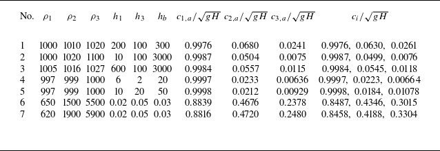
, which are compatible with the inequalities of (5.14), and of course with all kind of realistic physical data. Therefore, it is expected that the approximate formulas perform best in this case. Nevertheless, the results in table 1 show that (5.28), (5.31) and (5.33) perform quite well also in (5.15) and (5.16).


The approximate and exact wave speeds for some values of the parameters. Rows 1 and 2 correspond to internal waves, row 3 refers to equatorial internal waves, rows 4 and 5 pertain to three-layer lakes, and rows 6 and 7 refer to laboratory experiments. The dimensionalities of all quantities are given in the International System of Units (SI),
 $g=9.81$
m s−2. All velocities are given in non-dimensional units by division by
 $\sqrt {gH}$
. The quantities
 $c_i$
are the positive roots of (5.1).

Remark 5.2. The two-layer limit case
 $\rho _3 =\rho _2$
, with depths
 $h_1$
and
 $h$
in (5.28) leads to
 \begin{align} c_{1,a}^*=\pm \sqrt {g(h_1+h)\left (1-\frac { h_1 h}{(h_1+h)^2} \frac {\rho _2-\rho _1}{\rho _2} \right )}. \end{align}
This appears also in e.g.Craig et al. (Reference Craig, Guyenne, Nicholls and Sulem2005)and Kodaira et al. (Reference Kodaira, Waseda, Miyata and Choi2016).
Remark 5.3. The two-layer limit case
 $\rho _3 =\rho _2$
, with depths
 $h_1$
and
 $h$
in (5.31), leads to the well-known formula for the phase speed of an internal wave, which is related to the so-called Brunt–Väisälä frequency,
 \begin{align} c^*_{2,a}=\pm \sqrt {\frac {g (\rho _2 - \rho _1) h h_1 }{\rho _2(h+h_1)} }. \end{align}
As a matter of fact, the precise formula for two layers in the rigid lid approximation is formula (4.5) of Craig et al. (Reference Craig, Guyenne, Nicholls and Sulem2005), but because in the ocean the two densities are very close (
 $\rho _1 \approx \rho _2$
), in many situations (5.35) is used instead (Massel Reference Massel2015
; Kodaira et al. Reference Kodaira, Waseda, Miyata and Choi2016
).
The propagation speed (5.31) is associated with the disturbance described by
 $\eta _2$
because the internal wave formed at this interface usually has a significant amplitude moving with the mentioned speed. Clearly,
 $\sqrt {gH}$
is the speed of the surface waves (over the total depth
 $H$
) which due to the influence of the interfaces is modified to (5.28), while (5.33) is the speed of internal waves, observable at the interface
 $y=\eta _3$
. In general, waves with all possible speeds have their traces on the surface and on both interfaces. However, their amplitudes can be of quite different magnitudes.
Table 1 displays a comparison between the solutions of the approximate formulas above and the (positive) numerical solutions of (5.1). It is remarkable that the approximate formulas (5.28)–(5.33) give a very good approximation (for a range of physically feasible values of the parameters) to the actual solutions of (5.1). Rows 1–6 of table 1 correspond to (5.14), and the approximation formulas provide very good approximations. Row 7 illustrates (5.15). It does not seem that there are any real-life examples satisfying case (5.16). The cases (5.15) and (5.16) exhibit very large differences in the densities, and are not realistic in an oceanographic context. The approximation formulas work less well in the examples that exhibit large density contrasts, but nevertheless the approximate values are very good as a guide to the locations of the exact ones.
The first example in table 1 reflects typical parameter values for interfacial ocean internal waves. The next example (shown as no. 2 in table 1) concerns oceanographic and limnological systems, where stratified water columns are common due to variations in temperature, salinity and pressure. A three-layer structure with densities approximately 1000, 1020 and 1100 kg m−3, and respective thicknesses 10, 100 and 3000 m, can be justified by combining observations from coastal, open ocean and hypersaline environments; cf. https://oceanexplorer.noaa.gov/technology/ctd/ctd.html, https://www.bodc.ac.uk/data/bodc_database/ctd/, https://podaac.jpl.nasa.gov/dataset/OMG_L2_CTD.
The third example (no. 3 in table 1) is with parameter values, typical for the internal equatorial waves in the Pacific Ocean; see e.g. Constantin & Ivanov (Reference Constantin and Ivanov2019). The total depth of the Pacific Ocean is approximately 4000 m on average, and the upper layer is several hundred metres deep. We note that standard seawater density rarely exceeds 1050
 $\rm kg\,m^{- 3}$
.
The next two examples (nos 4 and 5 in table 1) of a three-layer system concern temperate lakes, in which – particularly during the summer stratification period – the water column consistently organises into three distinct layers: the epilimnion, metalimnion and hypolimnion. The epilimnion, which typically extends from the surface to depths of 5–20 m, is a warm, well-mixed layer influenced by wind and solar heating. Beneath it lies the metalimnion, or thermocline, a transition zone several metres thick, where temperature and density change rapidly with depth, effectively inhibiting vertical mixing. The hypolimnion, the coldest and densest layer, lies below the thermocline and remains largely isolated from surface influences, often becoming oxygen-depleted over time because of biological activity and lack of mixing. This three-layer structure is not just a convenient simplification, but a physically necessary framework that accurately captures the thermal, chemical and biological dynamics of stratified lakes. Unlike oceanographic systems, where stratification is governed by both temperature and salinity over much greater depths, lake stratification is shallow, thermally driven and seasonally reversible, reflecting the unique density behaviour of freshwater and the limited depth of most inland water bodies (cf. Huttula Reference Huttula, Bengtsson, Herschy and Fairbridge2012).
To investigate flow behaviour in sharply stratified systems, we consider (in rows 6 and 7 of table 1) a three-layer fluid column with engineered density contrasts that far exceed those found in natural oceanographic environments (see National Institute of Standards and Technology, US Department of Commerce, NIST Chemistry WebBook, SRD 69). Unlike ocean stratification, which typically involves density differences of only 1–3
 $\%$
due to temperature and salinity gradients, this system spans nearly an order of magnitude in density, using immiscible or semi-miscible fluids to maintain stable, well-defined interfaces.
The top layer typically consists of light hydrocarbons such as pentane or hexane. These fluids have densities in the range 600–700
 $\rm kg\,m^{- 3}$
and form a buoyant, sharply defined upper boundary. In experimental set-ups, this layer is often kept relatively thin, with height approximately 1–2 cm, to minimise mixing and maintain interface clarity.
The middle layer is composed of dense aqueous solutions, such as
 $\rm ZnCl_2$
brines or glycerol–water mixtures, with densities in the range 1000–2200
 $\rm kg\,m^{- 3}$
. This layer serves as a transitional buffer and is typically the thickest, with heights 3–5 cm, allowing for stable stratification and tunable flow dynamics. Its density can be adjusted to fine-tune the separation between the top and bottom layers.
The bottom layer features ultra-dense fluids such as perfluorodecalin, or liquid metals such as gallium alloys, which can reach densities 6400
 $\rm kg\,m^{- 3}$
. This layer is usually 1–3 cm thick and provides a heavy, immiscible foundation that anchors the system and prevents upward mixing.
6. The limit to two layers with a free surface
We show here that the dispersion relation for the two-layer case, known from previous works of Lamb (Reference Lamb1932) and Craig et al. (Reference Craig, Guyenne, Nicholls and Sulem2005), follows from considerations about the three-layer setting, as a particular case of (4.20). In this case, we set
 $\rho _3=\rho _2$
. Then taking into account (4.9) and (4.10), we have
 \begin{align} \begin{split} &A^0_{11} = k\frac {\tanh (kh) \coth (kh_1)+ {\rho _2}/{\rho _1}}{\rho _2 \coth (k h_1) + \rho _1 \tanh (kh)},\\ &A^0_{12} = k\frac {\tanh (kh) }{\sinh (kh_1)\big (\rho _2 \coth (k h_1) + \rho _1 \tanh (kh)\big )} ,\\ &A^0_{22} = k\frac {\tanh (kh) \coth (kh_1) }{\rho _2 \coth (k h_1) + \rho _1 \tanh (kh)}.\\ \end{split} \end{align}
Therefore, expanding the determinant of the matrix
 $\mathcal{M}(k)-\lambda I_6$
by row three, we obtain
 \begin{align} \textrm {det}(\mathcal{M}(k)-\lambda I_6)=\lambda ^2\big [\lambda ^4-(b_1 A^0_{11}+b_2 A^0_{22})\lambda ^2+b_1 b_2\big (A^0_{11} A^0_{22}-(A^0_{12})^2\big )\big ]. \end{align}
Further, we find from (6.1) that
 \begin{align} b_1 A^0_{11}+b_2 A^0_{22}=-g\rho _2 k\frac {1+\tanh (kh)\coth (kh_1)}{\rho _2\coth (kh_1)+\rho _1\tanh (kh)}, \\[-12pt] \nonumber \end{align}
 \begin{align} b_1 b_2\big (A^0_{11} A^0_{22}-(A^0_{12})^2)=\frac {g^2(\rho _2-\rho _1)k^2\tanh (kh_1)\tanh (kh)}{\rho _2+\rho _1\tanh (kh_1)\tanh (kh)}. \\[9pt] \nonumber \end{align}
Proceeding as before, i.e. searching for solutions
 $\hat {u}=\hat {u}_0\, \mathrm{e}^{\mathrm{i}k(x-ct)}$
in (4.14) and denoting
 $\omega (k):=ck$
, which is the spatial frequency of the wave solution, we notice from (6.2) and (6.3) that
 $\omega$
satisfies the equation
 \begin{align} \omega ^4-g\rho _2 k\frac {1+\tanh (kh)\coth (kh_1)}{\rho _2\coth (kh_1)+\rho _1\tanh (kh)}\omega ^2+ \frac {g^2(\rho _2-\rho _1)k^2\tanh (kh_1)\tanh (kh)}{(\rho _2+\rho _1\tanh (kh_1)\tanh (kh))}=0, \end{align}
i.e. we recover the equation obtained by Craig et al. (Reference Craig, Guyenne, Nicholls and Sulem2005) with Hamiltonian methods. This equation apparently goes back to Lamb (Reference Lamb1932), where the problem of ‘superimposed liquids’ is solved.
Remark 6.1. Denoting
 $\omega ^2:=Y$
, we observe that
 $Y$
satisfies a second-degree algebraic equation whose discriminant is
 $\varDelta =(b_1 A_{11}-b_2 A_{22})^2+4b_1 b_2(A_{12})^2\gt 0$
, which shows that this equation has two real roots, called
 $Y_1,Y_2$
. Since
 \begin{align} Y_1+Y_2=g\rho _2 k\frac {1+\tanh (kh)\coth (kh_1)}{\rho _2\coth (kh_1)+\rho _1\tanh (kh)}\gt 0, \\[-12pt] \nonumber \end{align}
 \begin{align} Y_1 \boldsymbol{\cdot} Y_2=\frac {g^2(\rho _2-\rho _1)k^2\tanh (kh_1)\tanh (kh)}{\rho _2+\rho _1\tanh (kh_1)\tanh (kh)}\gt 0, \\[9pt] \nonumber \end{align}
 $w$
e infer that
 $Y_1$
and
 $Y_2$
are positive, i.e. (6.4) has four real roots.
7. The rigid lid model
In this section, we discuss the rigid lid model, which corresponds to a flat surface
 $\eta _1(x,t)\equiv 0$
. The difference from the model with a non-trivial free surface is that for the domain
 $\varOmega _1$
of the upper layer, we have a single DN operator, namely
 $G_1(\eta _2)$
.
7.1. The DN operators and evolution equations
We use the techniques developed in the previous sections and repeat the same steps. The Hamiltonian formulation can be established in this case as well; however, we are going to employ only techniques related to the DN operators. For the middle and lower layers, we have the DN operators (3.22) and (3.23). The DN operator for the upper layer is as in (2.12) of Craig et al. (Reference Craig, Guyenne, Nicholls and Sulem2005) and is defined as
 \begin{align} \left ( \frac {\partial \varphi _1}{\partial (-\boldsymbol {n}_2)} \right )_{s_2}\sqrt {1+\eta _{2,x}^2}=-{\boldsymbol {n}_2}\boldsymbol{\cdot }(\boldsymbol{\nabla }\varphi _1)_{s_2} \equiv - G_1(\eta _2) (\varphi _1)_{s_2}. \end{align}
More details are provided in (A.10) of Craig et al. (Reference Craig, Guyenne, Nicholls and Sulem2005), e.g.
 \begin{align} G_1(\eta _2)=\sum _{l=0}^{\infty }G_1^{(l)}(\eta _2), \\[-28pt] \nonumber \end{align}
 \begin{align} G_1^{(0)}= D \tanh (h_1 D), \quad G_1^{(1)}=- D \eta _2(x)\, D + G_1^{(0)}\, \eta _2(x)\, G_1^{(0)} +\cdots . \\[2pt] \nonumber \end{align}
Then obviously
 \begin{align} \eta _{2,t}=- G_1(\eta _2) (\varphi _1)_{s_2}=\varGamma _{11}(\varphi _2)_{s_2}+\varGamma _{12}(\varphi _2)_{s_3}, \end{align}
and as in (3.27), we obtain
 \begin{align} \eta _{3,t}=G(\eta _3)(\varphi _3)_{s_3}=-[\varGamma _{21}(\varphi _2)_{s_2}+\varGamma _{22}(\varphi _2)_{s_3}]. \end{align}
Equations (7.4) and (7.5) together with
 \begin{align} \xi _2:=\rho _2(\varphi _2)_{s_2}-\rho _1(\varphi _1)_{s_2}, \quad \xi _3:=\rho _3(\varphi _3)_{s_3}-\rho _2(\varphi _2)_{s_3} \end{align}
can be solved for
 $(\varphi _1)_{s_2}$
,
 $(\varphi _2)_{s_2}$
,
 $(\varphi _2)_{s_3}$
and
 $(\varphi _3)_{s_3}$
in terms of
 $\xi _2,\xi_3$
and the corresponding DN operators (that depend on
 $\eta _2$
and
 $\eta _3$
). We obtain the following expressions (different from those in (3.35) and (3.36)):
 \begin{align} (\varphi _2)_{s_2}&=B^{-1}\big [ \rho _1 G \xi _3 + (\rho _3 \varGamma _{22}+\rho _2 G) \varGamma _{12}^{-1} G_1 \xi _2 \big ]=:\varPhi ^2_2(\eta _i, \xi _i) , \\[-12pt] \nonumber \end{align}
 \begin{align} (\varphi _2)_{s_3}&=-(B^*)^{-1}\big [ \rho _3 G_1 \xi _2 + (\rho _1 \varGamma _{11}+\rho _2 G_1) \varGamma _{21}^{-1} G \xi _3 \big ]=:\varPhi ^2_3(\eta _i, \xi _i), \\[9pt] \nonumber \end{align}
where
 \begin{align} B= (\rho _3 \varGamma _{22}+\rho _2 G) \varGamma _{12}^{-1}(\rho _2 G_1+\rho _1 \varGamma _{11})-\rho _1\rho _3 \varGamma _{21}. \end{align}
This allows to express (7.4) and (7.5) in the form
 \begin{align} \eta _{2,t}&= A_{22}\xi _2+A_{23} \xi _3, \\[-12pt] \nonumber \end{align}
 \begin{align} \eta _{3,t}&= A_{32}\xi _2+A_{33} \xi _3 , \\[9pt] \nonumber \end{align}
where
 \begin{align} A_{22}&=-\rho _3 \varGamma _{12} (B^*)^{-1} G_1+ \varGamma _{11} B^{-1}(\rho _3 \varGamma _{22}+\rho _2 G) \varGamma _{12}^{-1} G_1, \\[-12pt] \nonumber \end{align}
 \begin{align} A_{23}&=\rho _1 \varGamma _{11} B^{-1} G -\varGamma _{12} (B^*)^{-1}(\rho _1 \varGamma _{11}+\rho _2 G_1) \varGamma _{21}^{-1} G, \\[-12pt] \nonumber \end{align}
 \begin{align} A_{32}&= \rho _3 \varGamma _{22} (B^*)^{-1} G_1 -\varGamma _{21} B^{-1}(\rho _3 \varGamma _{22}+\rho _2 G) \varGamma _{12}^{-1} G_1, \\[-12pt] \nonumber \end{align}
 \begin{align} A_{33}&=-\rho _1 \varGamma _{21} B^{-1} G +\varGamma _{22} (B^*)^{-1}(\rho _1 \varGamma _{11}+\rho _2 G_1) \varGamma _{21}^{-1} G \\[9pt] \nonumber \end{align}
are operators that depend only on
 $\eta _2$
and
 $\eta _3$
. These operators, of course, are not the same as those in (3.38). Thus defining
 \begin{align} F_2(\eta _i, \xi _i):= A_{22}\xi _2+A_{23} \xi _3, \quad F_3(\eta _i, \xi _i):=A_{32}\xi _2+A_{33} \xi _3 , \quad i=2,3, \end{align}
we have the nonlinear dynamics for
 $\eta _2$
and
 $\eta _3$
from (7.4) in the form
 \begin{align} \eta _{2,t}= F_2(\eta _i, \xi _i), \quad \eta _{3,t}=F_3(\eta _i, \xi _i), \end{align}
and also
 \begin{align} (\varphi _1)_{s_2}&=-G_1^{-1}\eta _{2,t}=-G_1(\eta _2)^{-1}F_2(\eta _i, \xi _i)=:\varPhi ^1_2(\eta _i, \xi _i), \\[-12pt] \nonumber \end{align}
 \begin{align} (\varphi _3)_{s_3}&=G^{-1}\eta _{3,t}=G(\eta _3)^{-1}F_3(\eta _i, \xi _i)=:\varPhi ^3(\eta _i, \xi _i). \\[9pt] \nonumber \end{align}
The time evolution of
 $\xi _2$
and
 $\xi _3$
is given by (3.53) and (3.55) as
 \begin{align} \xi _{2,t}&+\frac {\rho _2 (\varPhi ^2_{2,x})^2-\rho _1 (\varPhi _{2,x}^1)^2-2F_2\xi _{2,x}\eta _{2,x}+(\rho _1-\rho _2)F_2^2 }{2(1+\eta _{2,x}^2)}+(\rho _2-\rho _1)g \eta _2 =0, \\[-12pt] \nonumber \end{align}
 \begin{align} \xi _{3,t}&+\frac {\rho _3 (\varPhi ^3_{x})^2-\rho _2 (\varPhi _{3,x}^2)^2-2F_3\xi _{3,x}\eta _{3,x}+(\rho _2-\rho _3)F_3^2 }{2(1+\eta _{3,x}^2)}+(\rho _3-\rho _2)g \eta _3 =0, \\[9pt] \nonumber \end{align}
with the new definitions of
 $F_2,F_3$
in (7.16), and the quantities in (7.7), (7.8), (7.18) and (7.19).
Thus we have the full nonlinear system of the time evolution in terms of DN operators given by (7.17), (7.20) and (7.21). We will illustrate how this system produces model equations in different propagation regimes.
7.2. Leading-order linear approximation and dispersion relation
In the leading-order approximation, we are using the DN operators from (7.3), (4.8) and (4.7) to obtain
 \begin{align} A_{22}^0(k)&= \frac {k[\rho _2 \cosh (kh_3)\sinh (kh_b) + \rho _3 \sinh (kh_3)\cosh (kh_b)]\sinh (k h_1)}{ \boldsymbol {D}(k) }, \\[-12pt] \nonumber \end{align}
 \begin{align} A_{23}^0(k)&=A_{32}^0(k)= \frac {k \rho _2 \sinh (k h_b)\sinh (k h_1) }{ \boldsymbol {D}(k) }, \\[-12pt] \nonumber \end{align}
 \begin{align} A_{33}^0(k)&= \frac {k[\rho _1 \cosh (k h_1) \sinh (kh_3) + \rho _2 \cosh (kh_3)\sinh (kh_1)]\sinh (k h_b)}{ \boldsymbol {D}(k) }, \\[9pt] \nonumber \end{align}
where
 \begin{align} \begin{split} \boldsymbol {D}(k)={}& \rho _2\Big (\rho _3 \cosh (k h_3) \cosh (k h_b)+\rho _2 \sinh (kh_3)\sinh (kh_b)\Big )\sinh (kh_1) \\ & {}+ \rho _1\Big (\rho _2 \cosh (k h_3) \sinh (k h_b)+\rho _3 \sinh (kh_3)\cosh (kh_b)\Big )\cosh (kh_1). \end{split} \end{align}
Note that for
 $k\ne 0$
, the sign of
 $\boldsymbol {D}(k)$
coincides with the sign of
 $k$
, thus
 $\boldsymbol {D}(k)\ne 0$
. The equations for
 $\xi _i$
are as in (4.13), and the linearised equations in the leading-order approximation therefore are
 \begin{align} \eta _{2,t}&=A^0_{22}(D)\,\xi _2+A^0_{23}(D)\, \xi _3, \\[-12pt] \nonumber \end{align}
 \begin{align} \eta _{3,t}&=A_{32}^{0}(D)\,\xi _2+A^0_{33}(D)\,\xi _3, \\[-12pt] \nonumber \end{align}
 \begin{align} \xi _{2,t}&=-g(\rho _2-\rho _1)\eta _2, \\[-12pt] \nonumber \end{align}
 \begin{align} \xi _{3,t}&=-g(\rho _3-\rho _2)\eta _3. \\[9pt] \nonumber \end{align}
The analogue of the matrix
 $\mathcal{M}$
in (4.14) is now
 \begin{align} \mathcal{M}(k)=\begin{pmatrix} 0 & 0 & A^0_{22}(k) & A^0_{23}(k)\\[5pt] 0 & 0 & A^0_{23}(k) & A^0_{33}(k)\\[5pt] g(\rho _1-\rho _2) & 0 & 0 &0 \\[5pt] 0 & g(\rho _2-\rho _3) & 0 & 0 \end{pmatrix}\!. \end{align}
The characteristic equation
 $\textrm {det} (\mathcal{M}(k)+ikcI_4)=0$
leads to the following bi-quadratic equation for the propagation speeds
 $c$
:
 \begin{align} &c^4 + a_2 c^2 +a_0 =0, \\[-12pt] \nonumber \end{align}
 \begin{align} a_2&=-\frac {g(A^0_{22}(\rho _2 - \rho _1) + A^0_{33}(\rho _3-\rho _2)) }{k^2}=-\frac {g\, \boldsymbol {D}_1(k)}{k\,\boldsymbol {D}(k)}, \\[-12pt] \nonumber \end{align}
 \begin{align} a_0&= \frac {g^2(\rho _3 - \rho _2)(\rho _2 - \rho _1)(A^0_{22}A^0_{33} - (A^0_{23})^2)}{k^4} \nonumber \\ & = \frac {g^2(\rho _3 - \rho _2)(\rho _2 - \rho _1)\sinh (kh_1)\sinh (kh_3)\sinh (k h_b)}{k^2\, \boldsymbol {D}(k)}, \\[9pt] \nonumber \end{align}
where
 \begin{align} \boldsymbol {D}_1(k)={}& [\rho _2(\rho _3-\rho _1)\cosh (k h_3) \sinh (k h_b) \nonumber \\&{}+ \rho _3(\rho _2-\rho _1) \sinh (kh_3)\cosh (kh_b)]\sinh (k h_1) \nonumber \\ &{}+\rho _1(\rho _3-\rho _2)\cosh (kh_1) \sinh (kh_3)\sinh (k h_b). \end{align}
7.3. Short-wave limit
The short-wave limit for the solutions of (7.31) can be obtained in a similar way by the asymptotics
 $\sinh (k h_i) \sim \pm (1/2)\exp (kh_i)$
and
 $ \cosh (k h_i) \sim (1/2)\exp (k h_i)$
for
 $k\to \pm \infty $
. Thus
 \begin{align} a_2 & \sim -\frac {g}{|k|} \left (\frac {\rho _2 - \rho _1}{\rho _2 + \rho _1}+ \frac {\rho _3-\rho _2}{\rho _3+\rho _2} \right )\!, \\[-12pt] \nonumber \end{align}
 \begin{align} a_0 & \sim \frac {g^2}{k^2} \left (\frac {\rho _2 - \rho _1}{\rho _2 + \rho _1}\right ) \left (\frac {\rho _3-\rho _2}{\rho _3+\rho _2}\right ) \!. \\[9pt] \nonumber \end{align}
The roots of (7.31) are real as well, and coincide with the two already known values in (4.29):
 \begin{align} c_{1}^2 \sim \frac {g}{|k|} \left (\frac {\rho _2 - \rho _1}{\rho _2 + \rho _1}\right )\! , \quad c_{2}^2 \sim \frac {g}{|k|} \left (\frac {\rho _3 - \rho _2}{\rho _3 + \rho _2}\right )\!. \end{align}
7.4. Long-wave limit
Passing to the long-wave limit
 $k\to 0$
gives
 \begin{align} a_2 & \to -g\frac {\rho _2(\rho _3-\rho _1) h_1 h_b + \rho _3(\rho _2-\rho _1) h_1 h_3 + \rho _1 (\rho _3-\rho _2) h_3 h_b}{\rho _2 \rho _3 h_1 + \rho _1 \rho _2 h_b + \rho _1 \rho _3 h_3}, \\[-12pt] \nonumber \end{align}
 \begin{align} a_0 & \to \frac {g^2(\rho _3 - \rho _2)(\rho _2 - \rho _1) h_1 h_3 h_b}{\rho _2 \rho _3 h_1 + \rho _1 \rho _2 h_b + \rho _1 \rho _3 h_3}, \\[9pt] \nonumber \end{align}
therefore we obtain the equation
 \begin{align} &(\rho _2 \rho _3 h_1 + \rho _1 \rho _2 h_b + \rho _1 \rho _3 h_3) c^4 \nonumber \\ &{}-g[\rho _2(\rho _3-\rho _1) h_1 h_b + \rho _3(\rho _2-\rho _1) h_1 h_3 + \rho _1 (\rho _3-\rho _2) h_3 h_b] c^2 \nonumber \\ & {}+g^2(\rho _3 - \rho _2)(\rho _2 - \rho _1) h_1 h_3 h_b=0, \end{align}
which appeared also in de Melo Viríssimo & Milewski (Reference de Melo Viríssimo and Milewski2019) and Ratliff (Reference Ratliff2022), where it is obtained by other methods. We will prove in the following that (7.40) has four real roots for all values of the densities and all values of the (mean) depths
 $h_1,h_3,h_b$
. To begin, we denote
 $c^2=Z$
in (7.40) and obtain the second-degree equation in
 $Z$
 \begin{align} (\rho _2 \rho _3 h_1 & + \rho _1 \rho _2 h_b + \rho _1 \rho _3 h_3) Z^2 \nonumber \\ & -g[\rho _2(\rho _3-\rho _1) h_1 h_b + \rho _3(\rho _2-\rho _1) h_1 h_3 + \rho _1 (\rho _3-\rho _2) h_3 h_b] Z \nonumber \\ & +g^2(\rho _3 - \rho _2)(\rho _2 - \rho _1) h_1 h_3 h_b=0. \end{align}
Taking into account that
 $\rho _3\gt \rho _2\gt \rho _1$
, and applying the Cauchy-Schwarz inequality, we have first
 \begin{align} &\rho _2(\rho _3-\rho _1) h_1 h_b + \rho _3(\rho _2-\rho _1) h_1 h_3 + \rho _1 (\rho _3-\rho _2) h_3 h_b \nonumber \\ &\geq 2h_1\sqrt {h_3 h_b}\sqrt {\rho _2\rho _3(\rho _3-\rho _1)(\rho _2-\rho _1)}\nonumber \\ & +2h_b\sqrt {h_1 h_3}\sqrt {\rho _1\rho _2(\rho _3-\rho _1)(\rho _3-\rho _2)}\nonumber \\ & +2h_3\sqrt {h_1 h_b}\sqrt {\rho _1\rho _3 (\rho _2-\rho _1)(\rho _3-\rho _2)}\nonumber \\ &\gt 2\sqrt {(\rho _3-\rho _2)(\rho _2-\rho _1)}\Big [\sqrt {\rho _2\rho _3}\,h_1\sqrt {h_3 h_b}+\sqrt {\rho _1\rho _2}\,h_b\sqrt {h_1 h_3}+\sqrt {\rho _1\rho _3}\,h_3\sqrt {h_1 h_b} \Big ]\nonumber \\ &=2\sqrt {(\rho _3-\rho _2)(\rho _2-\rho _1)}\sqrt {h_1 h_3 h_b}\Big [\sqrt {\rho _2\rho _3 h_1}+\sqrt {\rho _1\rho _2 h_b}+\sqrt {\rho _1\rho _3 h_3}\Big ]\nonumber \\ &\geq 2\sqrt {(\rho _3-\rho _2)(\rho _2-\rho _1)}\sqrt {h_1 h_3 h_b} \sqrt {\rho _2\rho _3 h_1+\rho _1\rho _2 h_b+\rho _1\rho _3 h_3}, \end{align}
where for the last inequality we have used that
 $\rho _i\ (i=1,2,3),\ h_1,h_3,h_b$
are positive. By squaring in the obtained inequality, we see that the discriminant of (7.41) is strictly positive, i.e. (7.41) has two distinct real roots, which, by the Viète formulas, are positive. From the latter finding we infer that the fourth-order equation (7.40) has four real roots: two positive and two negative.
We obtain an approximation for the smaller root by neglecting
 $c^4$
in (7.40),
 \begin{align} c_{-}:=\pm \sqrt {\frac {g(\rho _3 - \rho _2)(\rho _2 - \rho _1) h_1 h_3 h_b}{\rho _2(\rho _3-\rho _1) h_1 h_b + \rho _3(\rho _2-\rho _1) h_1 h_3 + \rho _1 (\rho _3-\rho _2) h_3 h_b }}, \end{align}
which in turn is approximately equal to (5.33) when
 $\rho _1 \approx \rho _2$
in the expression
 $ \rho _1 (\rho _3-\rho _2) h_3 h_b \approx \rho _2 (\rho _3-\rho _2) h_3 h_b$
.
By neglecting the last term in (7.40), we obtain an approximation for the larger root,
 \begin{align} c_{+}:=\pm \sqrt {\frac {g[\rho _2(\rho _3-\rho _1) h_1 h_b + \rho _3(\rho _2-\rho _1) h_1 h_3 + \rho _1 (\rho _3-\rho _2) h_3 h_b]}{\rho _2 \rho _3 h_1 + \rho _1 \rho _2 h_b + \rho _1 \rho _3 h_3}}. \end{align}
Under the further assumption that
 $\rho _1\approx \rho _2 \approx \rho _3 = \rho$
in the denominator and in the ratios
 $\rho _i/\rho _{\!j}$
, we have
 \begin{align} c_{+} &\approx \pm \sqrt {\frac {g[\rho _2(\rho _3-\rho _1) h_1 h_b + \rho _3(\rho _2-\rho _1) h_1 h_3 + \rho _1 (\rho _3-\rho _2) h_3 h_b]}{\rho ^2( h_1 + h_b + h_3)}} \nonumber \\ & \approx \pm \sqrt {\frac {g}{h_1+h} \left (\frac {(\rho _2-\rho _1) h_1 h_3}{\rho _2}+ \frac {(\rho _3-\rho _2) h_3 h_b}{\rho _3}+\frac {(\rho _3-\rho _1) h_1 h_b}{\rho _3} \right )} , \end{align}
which is (5.33).
Therefore the approximation formulas for both models agree under the further assumption of small relative differences between densities,
 $|\rho _i - \rho _{\!j}|/\rho _n \ll 1$
.
Finally, we point out that each propagation speed has its trace at every surface. For the largest propagation speed
 $c_+$
(mode 1), the ratio of the wave amplitudes
 $\eta _2,\eta_3$
of the upper and lower interfaces in the linear regime is
 $ ({\eta _2}/{\eta _3} )_{c=c_+} \gt 0$
. In this case, both waves have the same polarity. For the slow-propagating mode
 $c_-$
(mode 2),
 $ ({\eta _2}/{\eta _3} )_{c=c_-} \lt 0,$
and in this case the waves have the opposite polarity. See e.g. the details in de Melo Viríssimo & Milewski (Reference de Melo Viríssimo and Milewski2019).
7.5. Boussinesq regime for the rigid lid system
The next example of evolution equations arising from (7.17), (7.20) and (7.21) is the Boussinesq regime. As a result, we obtain a coupled system of nonlinear evolution equations. We recall the expansions of the DN operators in the case under consideration (Craig et al. Reference Craig, Guyenne, Nicholls and Sulem2005; Ivanov et al. Reference Ivanov, Martin and Todorov2022):
 \begin{align} G_1(\eta _2)={}& D\tanh (h_1D)-D\eta _2 D+D\tanh (h_1D)\, \eta _2 D\tanh (h_1D)+\cdots , \\[-12pt] \nonumber \end{align}
 \begin{align} G(\eta _3)={}& D\tanh (h_bD)+D\eta _3 D-D\tanh (h_b D)\, \eta _3 D\tanh (h_bD)+\cdots ,\\[-12pt] \nonumber \end{align}
 \begin{align} \varGamma _{11}(\eta _2, \eta _3)={}& D \coth (h_3D) + D\,{\textrm {csch}}(h_3D)\,\eta _3 D\,{\textrm {csch}} (h_3D) \nonumber \\ & {}+ D\eta _2D-D\coth (h_3D)\,\eta _2D\coth (h_3D)+\cdots ,\\[-12pt] \nonumber \end{align}
 \begin{align} \varGamma _{12}(\eta _2,\eta _3)={}& -D\,{\textrm {csch}}(h_3D)-D\,{\textrm {csch}}(h_3D)\,\eta _3 D\coth (h_3D) \nonumber \\ & {}+D \coth (h_3D)\,\eta _2 D\, {\textrm {csch}}(h_3D)+\cdots, \\[-12pt] \nonumber \end{align}
 \begin{align} \varGamma _{21}(\eta _2,\eta _3)={}& -D\,{\textrm {csch}}(h_3D) -D\coth (h_3D)\,\eta _3 D\, {\textrm {csch}}(h_3D) \nonumber \\ & {}+D\,{\textrm {csch}}(h_3D)\, \eta _2 D \coth (h_3D)+\cdots ,\\[-12pt] \nonumber \end{align}
 \begin{align} \varGamma _{22}(\eta _2, \eta _3)={}& D \coth (h_3D) + D\coth (h_3D)\,\eta _3 D\coth (h_3D) - D \eta _3 D \nonumber \\ & {}-D\,{\textrm {csch}}(h_3D)\, \eta _2 D\, {\textrm {csch}}(h_3D)+\cdots . \\[9pt] \nonumber\end{align}
We use these expansions in the Boussinesq regime, i.e. assuming that the small-amplitude parameters for each combination
 $\varepsilon _{\textit{ij}} = {|\eta _{\!j}|_{{max}}}/{h_i}$
are of the same order of magnitude, say
 $\varepsilon $
, for all
 $i,j$
, and also that the long-wave parameters
 $\delta _{\!j}={2 \pi h_{\!j}}/{\lambda }=k h_{\!j}$
are of the same order
 $\delta $
, and moreover
 $\varepsilon \ll 1$
and
 $ \delta ^2 \ll 1$
are of the same order as well. Furthermore, we recall the fact that the eigenvalue of
 $D$
is the wavenumber
 $k$
, so the action of
 $D$
will generate a quantity of order
 $\delta $
. On the other hand, the multiplication by
 $\eta _{\!j}$
will generate a quantity of order
 $\varepsilon$
. Keeping this in mind, the relevant expansion of (7.12)–(7.15) in terms of the DN operators (7.46)–(7.51) is
 \begin{align} A_{22}=A_{220}D^2 + A_{221}D^4+ B_{222} D\eta _2D+B_{223} D\eta _3 D +\cdots , \\[-12pt] \nonumber \end{align}
 \begin{align} A_{23}=A_{32}=A_{230}D^2 + A_{231}D^4+ B_{232} D\eta _2D+B_{233} D\eta _3 D +\cdots , \\[-12pt] \nonumber \end{align}
 \begin{align} A_{33}=A_{330}D^2 + A_{331}D^4+ B_{332} D\eta _2D+B_{333} D\eta _3 D +\cdots , \\[9pt] \nonumber \end{align}
where the expansion coefficients are
 \begin{align} & A_{220} = \frac {h_1(h_3\rho _3 + h_b\rho _2) }{ h_1\rho _2\rho _3+ h_3\rho _1 \rho _3 + h_b\rho _1\rho _2}, \\[-9pt] \nonumber \end{align}
 \begin{align} & A_{221}=- \dfrac {\begin{array}{c} h_1^2 \big(h_1h_3^2\rho _1\rho _3^2 + 2h_1h_3h_b\rho _1\rho _2\rho _3 + h_1h_b^2\rho _1\rho _2^2 + h_3^3\rho _2\rho _3^2 + 3h_3^2h_b\rho _2^2\rho _3 \big.\\\big. + 3h_3h_b^2\rho _2^3 + h_b^3\rho _2^2\rho _3\big)\end{array}}{3(h_1\rho _2\rho _3+ h_3\rho _1 \rho _3 + h_b\rho _1\rho _2)^2}, \\[-9pt] \nonumber \end{align}
 \begin{align} & B_{222}= \frac {-(h_3\rho _3 + h_b\rho _2)^2\rho _1 + h_1^2\rho _2\rho _3^2}{(h_1\rho _2\rho _3+ h_3\rho _1 \rho _3 + h_b\rho _1\rho _2)^2}, \\[-9pt] \nonumber \end{align}
 \begin{align} & B_{223}= \frac {(\rho _2-\rho _3)h_1^2\rho _2\rho _3 }{(h_1\rho _2\rho _3+ h_3\rho _1 \rho _3 + h_b\rho _1\rho _2)^2}, \\[-9pt] \nonumber \end{align}
 \begin{align} & A_{230}=\frac { h_1 h_b \rho _2}{h_1\rho _2\rho _3+ h_3\rho _1 \rho _3 + h_b\rho _1\rho _2} , \\[-9pt] \nonumber \end{align}
 \begin{align} & A_{231} = - \dfrac { \begin{array}{c} h_1 h_b \rho _2\big[6h_1h_bh_3 \rho _2^2+ h_b(2h_1^2 + 3 h_3^2)\rho _1\rho _2 + (3 h_3^2 + 2h_b^2)h_1\rho _2\rho _3 \big.\\ + \big. h_3(2h_1^2 + h_3^2 +2 h_b^2)\rho _1\rho _3 \big]\end{array}}{6(h_1\rho _2\rho _3 + h_3\rho _1 \rho _3 + h_b\rho _1\rho _2)^2} , \\[-9pt] \nonumber \end{align}
 \begin{align} & B_{232}= -\frac {h_b \rho _1 \rho _2 [h_b \rho _2 + (h_1 + h_3)\rho _3] }{( h_1\rho _2\rho _3+ h_3\rho _1 \rho _3 + h_b\rho _1\rho _2 )^2 } , \\[-9pt] \nonumber \end{align}
 \begin{align} & B_{233}=\frac {h_1 \rho _3\rho _2 [(h_3 + h_b)\rho _1 + h_1 \rho _2 ]}{( h_1\rho _2\rho _3+ h_3\rho _1 \rho _3 + h_b\rho _1\rho _2)^2}, \\[9pt] \nonumber\end{align}
 \begin{align} & A_{330}=\frac {h_b(h_1\rho _2 + h_3\rho _1)}{h_1\rho _2\rho _3+ h_3\rho _1 \rho _3 + h_b\rho _1\rho _2} \\[-9pt] \nonumber \end{align}
 \begin{align} & A_{331}\nonumber \\ &=-\frac {\begin{array}{c} h_b^2 \big(h_1^3\rho _1\rho _2^2 + 3h_1^2h_3\rho _2^3 + h_1^2h_b\rho _2^2\rho _3 + 3h_1h_3^2\rho _1\rho _2^2 + 2h_1h_3h_b\rho _1\rho _2\rho _3 + h_3^3\rho _1^2\rho _2 \big.\\ \big. + h_3^2h_b\rho _1^2\rho _3 \big)\end{array}}{3(h_1\rho _2\rho _3+ h_3\rho _1 \rho _3 + h_b\rho _1\rho _2)^2}, \\[-9pt] \nonumber \end{align}
 \begin{align} & B_{332}=\frac {h_b^2(\rho _1 -\rho _2)\rho _1\rho _2}{(h_1\rho _2\rho _3+ h_3\rho _1 \rho _3 + h_b\rho _1\rho _2)^2}, \\[-9pt] \nonumber \end{align}
 \begin{align} & B_{333}=\frac {(h_1\rho _2 + h_3\rho _1)^2\rho _3 - h_b^2\rho _1^2\rho _2}{(h_1\rho _2\rho _3+ h_3\rho _1 \rho _3 + h_b\rho _1\rho _2)^2}. \\[9pt] \nonumber \end{align}
Since in the Boussinesq regime the equations are maximum quadratic in the field variables, (7.20) and (7.21) suggest that we need only the leading order of the quantities
 $\varPhi ^i_{\!j}$
and
 $F_{\!j}$
:
 \begin{align} \varPhi ^2_2=&\frac {h_1\rho _3\xi _2 - h_b\rho _1\xi _3}{h_1\rho _2\rho _3+ h_3\rho _1 \rho _3 + h_b\rho _1\rho _2}, \\[-12pt] \nonumber \end{align}
 \begin{align} \varPhi ^1_2=&-\frac {h_b \rho _2 (\xi _2 + \xi _3) + h_3\rho _3\xi _2}{h_1\rho _2\rho _3+ h_3\rho _1 \rho _3 + h_b\rho _1\rho _2}, \\[-12pt] \nonumber \end{align}
 \begin{align} \varPhi ^3=&\frac {h_1 (\xi _2 +\xi _3)\rho _2 + h_3 \xi _3\rho _1}{h_1\rho _2\rho _3+ h_3\rho _1 \rho _3 + h_b\rho _1\rho _2} , \\[-12pt] \nonumber \end{align}
 \begin{align} \varPhi ^2_3=&\frac {h_1\rho _3\xi _2 - h_b\rho _1\xi _3}{h_1\rho _2\rho _3+ h_3\rho _1 \rho _3 + h_b\rho _1\rho _2}. \\[9pt] \nonumber \end{align}
Introducing the variables
 $\mathfrak{u}_{\!j}=(\xi _{\!j})_x$
, we first notice that
 $F_{\!j}$
in leading order are linear combinations of
 $\mathfrak{u}_{j,x}$
, while
 $\varPhi ^i_{j,x}$
are linear combinations of
 $\mathfrak{u}_{j}$
only. However, we notice that
 $\mathcal{O}(h_{\!j} \mathfrak{u}_{j,x}) = \mathcal{O}(kh_{\!j} \mathfrak{u}_{j}) = \delta\, \mathcal{O}(\mathfrak{u}_{j})\ll \mathcal{O}(\mathfrak{u}_{j})$
. Thus the terms with
 $F_{\!j}$
in (7.20) and (7.21) can be neglected in comparison to the other terms with
 $\varPhi ^i_{j,x}$
(as in the water wave theory of a single layer). Then we obtain the system
 \begin{align} \mathfrak{u}_{2,t} & + \frac {[\rho _2(h_1\rho _3\mathfrak{u}_2 - h_b\rho _1\mathfrak{u}_3)^2-\rho _1(h_b \rho _2 (\mathfrak{u}_2 + \mathfrak{u}_3) + h_3\rho _3\mathfrak{u}_2)^2]_x}{2(h_1\rho _2\rho _3+ h_3\rho _1 \rho _3 + h_b\rho _1\rho _2)^2} +(\rho _2-\rho _1)g\eta _{2,x}=0 , \nonumber \\\mathfrak{u}_{3,t} &+ \frac {[\rho _3(h_1 \rho _2 (\mathfrak{u}_2 +\mathfrak{u}_3) + h_3 \rho _1 \mathfrak{u}_3 )^2-\rho _2(h_1\rho _3\mathfrak{u}_2 - h_b\rho _1\mathfrak{u}_3)^2]_x}{2(h_1\rho _2\rho _3+ h_3\rho _1 \rho _3 + h_b\rho _1\rho _2)^2} +(\rho _3-\rho _2)g\eta _{3,x}=0, \nonumber\\\eta _{2,t} & = -A_{220}\mathfrak{u}_{2,x} + A_{221}\mathfrak{u}_{2,\textit{xxx}}- B_{222} [\eta _2 \mathfrak{u}_{2}]_x -B_{223} [\eta _3 \mathfrak{u}_{2} ]_x \nonumber\\&{}-A_{230} \mathfrak{u}_{3,x} + A_{231}\mathfrak{u}_{3,\textit{xxx}}- B_{232} [\eta _2 \mathfrak{u}_{3}]_x -B_{233} [\eta _3 \mathfrak{u}_{3} ]_x ,\nonumber\\\eta _{3,t} & = -A_{230}\mathfrak{u}_{2,x} + A_{231} \mathfrak{u}_{2,\textit{xxx}} - B_{232} [\eta _2 \mathfrak{u}_{2}]_x -B_{233} [\eta _3 \mathfrak{u}_{2} ]_x \nonumber\\& {}-A_{330}\mathfrak{u}_{3,x} + A_{331} \mathfrak{u}_{3,\textit{xxx}} - B_{332} [\eta _2 \mathfrak{u}_{3}]_x -B_{333} [\eta _3 \mathfrak{u}_{3} ]_x . \end{align}
Letting
 $\rho _1 \to 0$
, we obtain the two-layer domain with surface
 $y=\eta _2(x,t)$
and interface
 $y=\eta _3(x,t)$
, whereby the coefficients
 $A_{ijk}, B_{ijk}\ (i, j\in \{1,2\},\ k\in \{0,1,2,3\})$
are given by
 \begin{align} A_{220}& =\frac {h_3\rho _3 + h_b\rho _2}{ \rho _2\rho _3}, \quad A_{221} = - \frac { h_3^3 \rho _3^2 + 3h_3^2h_b\rho _2 \rho _3 + 3h_3h_b^2\rho _2^2 + h_b^3\rho _2 \rho _3}{3\rho _2 \rho _3 ^2}, \nonumber \\ B_{222}& = \frac {1}{\rho _2 },\quad B_{223} = \frac {\rho _2-\rho _3 }{\rho _2\rho _3 }, \nonumber \\ A_{230}& = \frac { h_b }{\rho _3 } ,\quad A_{231} = - \frac { h_b \big[6h_bh_3 \rho _2+ \big(3 h_3^2 + 2h_b^2 \big) \rho _3 \big]}{6 \rho _3^2} , \quad B_{232} = 0 ,\quad B_{233} = \frac { 1 }{\rho _3 }, \nonumber \\ A_{330}& = \frac {h_b }{\rho _3}, \quad A_{331} = -\frac {h_b^2 ( 3 h_3\rho _2 + h_b \rho _3 )}{3 \rho _3 ^2},\quad B_{332} = 0,\quad B_{333} =\frac {1}{\rho _3 }. \end{align}
Consequently, system (7.71) becomes
 \begin{align} \begin{split} \mathfrak{u}_{2,t}+{} &\frac {1}{ \rho _2 } \mathfrak{u}_2 \mathfrak{u}_{2,x} +\rho _2 g\eta _{2,x}=0 , \\ \mathfrak{u}_{3,t}+{} &\frac {\rho _2-\rho _3}{\rho _2 \rho _3 }\mathfrak{u}_2 \mathfrak{u}_{2 ,x} + \frac {1}{\rho _3}(\mathfrak{u}_2\mathfrak{u}_3)_x+ \frac {1}{\rho _3}\mathfrak{u}_3 \mathfrak{u}_{3 ,x} +(\rho _3-\rho _2)g\eta _{3,x}=0 ,\\ \eta _{2,t}={}&- \frac {h_3\rho _3 + h_b\rho _2}{ \rho _2\rho _3} \mathfrak{u}_{2,x} - \frac { h_3^3 \rho _3^2 + 3h_3^2h_b\rho _2 \rho _3 + 3h_3h_b^2\rho _2^2 + h_b^3\rho _2 \rho _3}{3\rho _2 \rho _3 ^2} \mathfrak{u}_{2,\textit{xxx}}\\ &{}-\frac {1}{\rho _2} [\eta _2 \mathfrak{u}_{2}]_x - \frac {\rho _2-\rho _3 }{\rho _2\rho _3 } [\eta _3 \mathfrak{u}_{2} ]_x \\ &{}- \frac { h_b }{\rho _3 } \mathfrak{u}_{3,x} - \frac { h_b \big[6h_bh_3 \rho _2+ \big(3 h_3^2 + 2h_b^2\big) \rho _3 \big]}{6 \rho _3^2} \mathfrak{u}_{3,\textit{xxx}} - \frac { 1 }{\rho _3 } [\eta _3 \mathfrak{u}_{3} ]_x ,\\ \eta _{3,t}={}&- \frac { h_b }{\rho _3 } \mathfrak{u}_{2,x} - \frac { h_b \big[6h_bh_3 \rho _2+ \big(3 h_3^2 + 2h_b^2\big) \rho _3 \big]}{6 \rho _3^2} \mathfrak{u}_{2,\textit{xxx}} - \frac { 1 }{\rho _3 } [\eta _3 \mathfrak{u}_{2} ]_x \\ & {}-\frac {h_b }{\rho _3} \mathfrak{u}_{3,x} -\frac {h_b^2 ( 3 h_3\rho _2 + h_b \rho _3 )}{3 \rho _3 ^2} \mathfrak{u}_{3,\textit{xxx}} - \frac {1}{\rho _3 }[\eta _3 \mathfrak{u}_{3} ]_x , \end{split} \end{align}
which recovers the system obtained by Craig et al. (Reference Craig, Guyenne, Nicholls and Sulem2005) on p. 1626, derived by employing similar methods involving expansions of the DN operators for two layers with a free surface.
The procedure utilised to obtain the Boussinesq system (7.73) highlights a general method for the derivation of nonlinear models for water waves propagation starting from the general system (7.17), (7.20) and (7.21).
7.6. Limit to the full equations for two layers with a free surface
The limit to the full equations for two layers with a free surface as they appear (however, in Hamiltonian form) in Craig et al. (Reference Craig, Guyenne, Nicholls and Sulem2005) could be done by simply setting up
 $\rho _1=0$
in all formulas in this section. Furthermore, given a depth
 $h^*$
, there is a relation between the DN operators
 $G_{\textit{ij}}(h^*, \eta _l, \eta _u)$
and
 $\varGamma _{\textit{ij}}(h^*, \eta _l, \eta _u)$
, which reads
 \begin{align} G_{11}(h^*, \eta _l, \eta _u)& =\varGamma _{22}(h^*, \eta _l, \eta _u) , \quad G_{12}(h^*, \eta _l, \eta _u)=\varGamma _{21}(h^*, \eta _l, \eta _u) , \\[-12pt] \nonumber \end{align}
 \begin{align} G_{21}(h^*, \eta _l, \eta _u)& =\varGamma _{12}(h^*, \eta _l, \eta _u) , \quad G_{22}(h^*, \eta _l, \eta _u)=\varGamma _{11}(h^*, \eta _l, \eta _u), \\[9pt] \nonumber \end{align}
where
 $y=\eta _l(x,t)$
is the lower boundary of the domain, and
 $y=\eta _u(x,t)$
is the upper boundary of the domain.
From (7.6), we obtain
 \begin{align} \xi _2:=\rho _2(\varphi _2)_{s_2} , \quad \xi _3:=\rho _3(\varphi _3)_{s_3}-\rho _2(\varphi _2)_{s_3}. \end{align}
We define the operator (essentially the operator
 $B$
in Craig et al. (Reference Craig, Guyenne, Nicholls and Sulem2005) for the free surface case.)
 \begin{align} \mathcal{B}:=\rho _3 \varGamma _{22}+\rho _2 G, \end{align}
which is self-adjoint. Then we have
 \begin{align} B^{-1}= \frac {1}{\rho _2}G_1^{-1}\varGamma _{12} \mathcal{B} ^{-1 }, \quad ( B^{-1})^*= \frac {1}{\rho _2} \mathcal{B} ^{-1 } \varGamma _{21}G_1^{-1 }. \end{align}
From (7.7) and (7.8), we obtain
 \begin{align} (\varphi _2)_{s_2}&=\frac {1}{\rho _2} \xi _2 =:\varPhi ^2_2(\xi _2) , \\[-12pt] \nonumber \end{align}
 \begin{align} (\varphi _2)_{s_3}&=-\mathcal{B} ^{-1 } \left [ G\xi _3 + \frac {\rho _3}{\rho _2} \varGamma _{21} \xi _2 \right ]=:\varPhi ^2_3(\eta _i, \xi _i). \\[9pt] \nonumber \end{align}
Then from (7.5), (7.79) and (7.80) after some calculations, we have
 \begin{align} (\varphi _3)_{s_3}=-G^{-1}[\varGamma _{21}(\varphi _2)_{s_2}+\varGamma _{22}(\varphi _2)_{s_3}]=\mathcal{B} ^{-1 } \left [-\varGamma _{21}\xi _2+\varGamma _{22}\xi _3 \right ]=:\varPhi ^3(\eta _i, \xi _i). \end{align}
In view of (7.74)–(7.75), these formulas reproduce (2.26)–(2.28) of Craig et al. (Reference Craig, Guyenne, Nicholls and Sulem2005). Next, from (7.12)–(7.15), we obtain the expressions for the operators:
 \begin{align} A_{22}&= \frac {1}{\rho _2}\varGamma _{11}-\frac {\rho _3}{\rho _2}\varGamma _{12}\mathcal{B} ^{-1 }\varGamma _{21}, \\[-12pt] \nonumber \end{align}
 \begin{align} A_{23}&= -\varGamma _{12}\mathcal{B} ^{-1 }G, \\[-12pt] \nonumber \end{align}
 \begin{align} A_{32}&= \frac {1}{\rho _2}\left (-\mathcal{B} +{\rho _3}\varGamma _{22}\right )\mathcal{B} ^{-1 }\varGamma _{21}=-G\mathcal{B} ^{-1 } \varGamma _{21}=A_{23}^* , \\[-12pt] \nonumber \end{align}
 \begin{align} A_{33}&= \varGamma _{22}\mathcal{B} ^{-1 }G. \\[9pt] \nonumber \end{align}
The operator
 $A_{33}$
is self-adjoint since
 $G$
and
 $\varGamma _{22}$
are self-adjoint operators (Craig et al. Reference Craig, Guyenne, Nicholls and Sulem2005). Indeed, we can write it formally as
 \begin{align} A_{33}=\frac {1}{\rho _3} \varGamma _{22}\left ( 1+\frac {\rho _2}{\rho _3} \varGamma _{22}^{-1} G \right )^{-1}\varGamma _{22}^{-1}G. \end{align}
In the leading order,
 $ ( {\rho _2}/{\rho _3})\,| \varGamma _{22}^{-1} G|= ({\rho _2}/{\rho _3})\, |{\tanh (kh_b)} \tanh (k h_3)|\lt 1$
, so, at least in some domain for the values of
 $(k,\eta _2,\eta _3)$
in the neighbourhood of
 $(0,0,0)$
, we have an expansion
 \begin{align} A_{33}=\frac {1}{\rho _3} \left ( G - \frac {\rho _2}{\rho _3} G \varGamma _{22}^{-1 }G + \frac {\rho _2^2}{\rho _3^2} G \varGamma _{22}^{-1 }G \varGamma _{22}^{-1 }G+\cdots \right )\!, \end{align}
from which it is evident that
 $A_{33}=A_{33}^*$
, thus
 $A_{33}= G \mathcal{B} ^{-1 } \varGamma _{22}$
. The operator
 $A_{22}$
is also self-adjoint since
 $\varGamma _{11}$
is self adjoint and
 $\varGamma _{12}^*=\varGamma _{21}$
; cf. Craig et al. (Reference Craig, Guyenne, Nicholls and Sulem2005).
The functionals
 $F_2$
and
 $F_3$
are as in (7.16); then the full equations of motion are the same as in (7.17), (7.20) and (7.21) (with
 $\rho _1=0$
), i.e. explicitly,
 \begin{align} \eta _{2,t}&=\left ( \frac {1}{\rho _2}\varGamma _{11}-\frac {\rho _3}{\rho _2}\varGamma _{12}\mathcal{B} ^{-1 }\varGamma _{21} \right ) \xi _2 -\varGamma _{12}\mathcal{B} ^{-1 }G \xi _3 =: F_2(\eta _i,\xi _i) , \end{align}
 \begin{align} \eta _{3,t}&= G\mathcal{B} ^{-1 }[ -\varGamma _{21} \xi _2+ \varGamma _{22} \xi _3]=:F_3(\eta _i, \xi _i), \end{align}
 \begin{align} \xi _{2,t}&=-\frac {\rho _2 (\varPhi ^2_{2,x})^2-2F_2\xi _{2,x}\eta _{2,x}-\rho _2F_2^2 }{2(1+\eta _{2,x}^2)}-\rho _2g \eta _2 , \end{align}
 \begin{align} \xi _{3,t}&=-\frac {\rho _3 (\varPhi ^3_{x})^2-\rho _2 (\varPhi _{3,x}^2)^2-2F_3\xi _{3,x}\eta _{3,x}+(\rho _2-\rho _3)F_3^2 }{2(1+\eta _{3,x}^2)}-(\rho _3-\rho _2)g \eta _3 . \end{align}
Equation (7.88) follows also from (7.4), (7.79) and (7.80); and (7.89) follows from (7.5) and (7.81). The DN operators depend on
 $\eta _2$
and
 $\eta _3$
in a complicated nonlinear way; however, as we have mentioned, there is a systematic approach for their derivation. In the Boussinesq limit, the above system produces the system (7.73) (see the derivation in Craig et al. Reference Craig, Guyenne, Nicholls and Sulem2005), although we have obtained it as a limit from (7.71). Figure 2 shows the relations between the derived models in this section.
Relations between the derived models: limits and approximations.

8. Conclusions and outlook
We have presented a Hamiltonian formulation for the nonlinear governing equations describing irrotational two-dimensional inviscid and incompressible water flows with piecewise constant density stratification in a three-layer fluid with a flat bottom, a free surface and two interfaces. We then introduced in each layer Dirichlet–Neumann (DN) operators with the help of which we re-expressed the Hamiltonian of the system and the equations of motion for the free surface and for the interfaces. The Hamiltonian formulation and the leading-order DN operators have allowed us to obtain linearised equations for small-amplitude waves at the surface and interfaces. We derived a bi-cubic equation representing the dispersion relation, in the short- and long-wave limits, we have analysed the solutions of this equation, and we obtained approximate expressions for the speed of the left- and right-running waves on the surface and at the internal interfaces.
The results presented here open new avenues of investigations, of which we mention a few.
-
(i) Formulas (3.30), (3.35) and (3.36) give (through the Hamiltonian variables) the boundary values of the velocity potential that extends analytically to the interior of the fluid body. This will lead to in-depth investigations of important properties of the flow pertaining to the pressure, velocity field and particle trajectories; cf. e.g. Henry & Villari (Reference Henry and Villari2022).
-
(ii) Since the three-layer scenario renders the inclusion of a current with piecewise linear profile more realistic and natural (as e.g. in Constantin et al. Reference Constantin, Ivanov and Martin2016; Constantin & Ivanov Reference Constantin and Ivanov2019), various results from the two-layer case concerning wave–current interactions in stratified flows are amenable to further extensions. In particular, the presence of currents in the layers will allow the formation of Kelvin–Helmholtz instabilities at the interfaces (see e.g. Benjamin & Bridges Reference Benjamin and Bridges1997a,Reference Benjamin and Bridgesb). In this case, the instability condition at each interface will incorporate the current components in the three layers, thereforedisplaying an increased level of complexity to the problem that will require the pursuit of significant new research in this direction.
-
(iii) Furthermore, a detailed study of the DN operators will lead to weakly nonlinear models for various propagation regimes that will be deduced from the equations presented in their general form; cf. (3.42), (3.43), (3.44), (3.53), (3.54), (3.55) in the case of a free surface, and (7.17), (7.20), (7.21) in the case of a flat surface. An example was given by the derivation of the coupled system (7.73) in the Boussinesq regime. From the weakly nonlinear regimes such as the Korteweg–de Vries regime, the soliton dynamics can be recovered, which is of practical importance given the fact that the solitons are stable and easier to observe in comparison to other wave types. The central role in the derivation of such systems is played by the DN operators and their expansions. Our motivation was based on the understanding that in the present research environment, the use of symbolic computation will increase dramatically (perhaps powered by AI), and the expansions of the DN operators should be highly facilitated.
The utilisation of the Hamiltonian formulation and the DN operators allows a concise derivation of model equations for this type of stratified flow. We have demonstrated how these equations can be written in an explicit final form for all scales and propagation regimes. If necessary, the expansions of the DN operators lead to particular equations for a specific (small) scale parameter (up to the desired order of the small parameter). For many configurations, especially the most common ones, these expansions are already known, which solves the problem immediately. Highlighting the significance of the DN operators, we point out that recent years have seen a surge in the study of both the full nonlinear water wave problem and various approximate nonlinear water wave models. This progress is driven by a combination of methods focusing on DN operators and Hamiltonian systems – cf. Baldi et al. (Reference Baldi, Berti, Haus and Montalto2018), Berti, Franzoi & Maspero (Reference Berti, Franzoi and Maspero2021), Bona, Lannes & Saut (Reference Bona, Lannes and Saut2008), Constantin & Ivanov (Reference Constantin and Ivanov2019), Clamond (Reference Clamond2022), Lannes (Reference Lannes2005), Alvarez-Samaniego & Lannes (Reference Alvarez-Samaniego and Lannes2008), Andrade & Nachbin (Reference Andrade and Nachbin2018), Ivanov et al. (Reference Ivanov, Martin and Todorov2022) – as well as methods for numerical computation of quantities, expressed by DN operators in Guyenne & Părău (Reference Guyenne and Părău2016), Guyenne (Reference Guyenne2017) and Canning Gregory & Nicholls (Reference Canning Gregory and Nicholls2012), following the pioneering work of Craig & Sulem (Reference Craig and Sulem1993).
Acknowledgements
The authors thank three anonymous reviewers and the editor (Prof. J. Kirby) for insightful comments and suggestions that significantly improved the paper.
Funding
R.I. gratefully acknowledges financial support from Research Ireland under grant no. 21/FFP-A/9150. C.I.M. acknowledges support from the project “Nonlinear studies of stratified oceanic and atmospheric flows”, funded by the European Union–NextGenerationEU and the Romanian Government under the National Recovery and Resilience Plan for Romania, contract no. 760040/23.05.2023, cod PNRR-C9-I8-CF 185/22.11.2022, through the Romanian Ministry of Research, Innovation and Digitalization, within Component 9, Investment I8.
Declaration of interests
On behalf of all authors, the corresponding author states that there is no conflict of interest.
Data availability statement
The reported results are of a purely theoretical nature, and no data have been used supporting these results.