2.1. One-dimensional limit

For one-dimensional propagation ( $Y=\partial /\partial b=0$ ) the continuity equation (2.12) becomes

With the help of (2.11), the free-surface condition (2.10a ) is then simplified to

This equation will be solved numerically for model validation in § 3.2. Note that in the constant water-depth case, i.e.  $h=h_{0}=1$ , (2.16) further reduces to

which was first given by Airy and is similar to the equation that governs the oscillations of nonlinear strings (Zabusky Reference Zabusky1962).

2.2. Linearized limit

Assuming that $\boldsymbol{X}\sim O({\it\epsilon})\ll 1$ the linearized form of (2.12), (2.10a ) and (2.10b ) is obtained as

Let us now consider that the seafloor deforms over time because of the passage of a landslide. Assuming this perturbation to be small we can rewrite the water depth as $h(x,y,t)=h_{0}(x,y)+f(x,y,t)$ where $f\sim O({\it\epsilon})$ . In this case, by Taylor expanding $h$ and substituting (2.18a ) in (2.11), the leading-order free-surface height is obtained as

where $\boldsymbol{{\rm\nabla}}_{h}=(\partial /\partial a,\partial /\partial b)$ . Taking the second time-derivative of (2.19), and using (2.18b ), (2.18c ) we obtain

Since ${\it\eta}=Z^{(0)}$ , $X=x-a\sim O({\it\epsilon})$ and $Y=y-b\sim O({\it\epsilon})$ , the above equation readily reduces to the classical shallow-water equation in the Eulerian frame of reference

Equation (2.21), first derived by Tuck & Hwang (Reference Tuck and Hwang1972), has an analytical closed-form solution in one- and two-dimensional setups (Liu, Lynett & Synolakis Reference Liu, Lynett and Synolakis2003; Sammarco & Renzi Reference Sammarco and Renzi2008; Didenkulova & Pelinovsky Reference Didenkulova and Pelinovsky2013).

2.3. Wave energy in a Lagrangian framework

To derive the expression for wave energy in terms of Lagrangian variables we first consider the Eulerian definition of wave energy (normalized by ${\it\rho}gH^{2}L^{2}$ ) in the domain ${\rm\Omega}=\{(x,y,z)\in \mathscr{F}(t)\times [-h(x,y,t),{\it\eta}(x,y,t)]\}$ where $\mathscr{F}(t)\subset \mathbb{R}^{2}$ is the horizontal projection of the free surface (that extends from one side’s runup or rundown to the other side’s runup or rundown):

Since ${\it\mu}=H/L\ll 1$ , we see from (2.22) that the contribution of the vertical velocity is negligible. The potential energy $\mathscr{E}_{\mathit{pot}}$ readily reduces to

Changing the variables of integration $(x,y,z)$ to the Lagrangian coordinates $(a,b,c)$ and noting that ${\it\eta}(x,y,t)=Z(a,b,0,t)$ , $\boldsymbol{x}_{t}=\boldsymbol{X}_{t}$ , we rewrite the total wave energy as

where clearly the determinant $\partial (x,y,z)/\partial (a,b,c)=1$ because of continuity. Note that $\mathscr{F}(0)$ is the projection of the initial (flat) water surface and therefore gives the limits of integration for the Lagrangian variables $a,b$ in (2.24). Also it is to be noted that the vertical limit of integration is from $-h_{0}(a,b)$ to 0, again because the integration is performed over Lagrangian variables. The final form of total wave energy is obtained once Airy’s expansion is substituted for the displacement variables. To the leading order, we get

3.1. Finite-difference scheme

We solve the system of equations (2.10) by the finite-difference method. Equations (2.10) are integrated in time using an explicit fourth-order method (Runge–Kutta 4) with $Z^{(0)}$ obtained from (2.11) and (2.12). A compact finite-difference Padé scheme is implemented to obtain the first- and second-order spatial derivatives such that the accuracy of the numerical scheme is that of a fourth-order method. The computation of the derivatives on the edges of the domain depends on the type of the boundary. For a vertical wall, which acts as a mirror, the normal displacement is zero, and the tangential displacement has a vanishing normal derivative. For a shoreline, which we define as the intersection of a sloping beach with the free surface, a forward or backward approximation is used in space to get the horizontal derivatives. The discretization of the derivatives on the boundaries is performed by adjusting the number of stencil points so that the order of approximation is the same as in the interior of the domain.

We shall assume perfect reflection at the shore and require the solution to be bounded everywhere including near the moving shoreline. Since for the linearized problem on a plane beach one of the homogeneous solutions is proportional to the Weber function $Y_{0}$ in two dimensions (Bessel functions of the second kind) and to the Whittaker function $W_{n^{2}/2m,0}$ in three dimensions ( $n,m\in \mathbb{N}$ ), which are both unbounded at the origin (see e.g. Shuto Reference Shuto1967, Reference Shuto1968), small errors in numerical approximations can induce instability. Indeed for the two-dimensional problem one obtains Bessel’s equation for a plane sloping beach, i.e. by substituting $h(a)=a\tan {\it\alpha}$ in (2.16), which presents a singularity at the shoreline $a=0$ . To resolve this issue numerically, we integrate the governing equations up to one grid cell before the shoreline. As a result, the physical shoreline is not part of the numerical domain, and is determined by a linear extrapolation from the grid boundary. The grid size is chosen small enough such that convergence is secured.

Table 1.

Comparison of wave runup extrema on an idealized beach ( $h(x)=x$ ) between: (i) numerical simulations of (2.16) and (ii) the analytical solution derived by Carrier et al. (Reference Carrier, Wu and Yeh2003) (in parentheses). The initial Gaussian waveform is described by (3.1) with amplitude $H_{1}=0.017/2$ for case  $\mathbf{a}^{\prime }$ and $H_{1}=0.017$ for case a. Other parameters are $c_{1}=4.0$ , $x_{1}=1.69$ . The analytical results for case a are the ones reported in Carrier et al. (Reference Carrier, Wu and Yeh2003) (with sign of the runup/rundown changed to correspond to runup heights instead of penetration depths), while those of case  $\mathbf{a}^{\prime }$ are based on a numerical integration of (2.9) in Kânoğlu (Reference Kânoğlu2004). The numerical simulations results are given for ${\it\delta}a=2\times 10^{-3}$ , ${\it\delta}t=4.88\times 10^{-5}$ .

3.2. Model validation

Numerical predictions of wave runup on a sloping beach based on our model equations are compared with analytical solutions of the celebrated hodograph-transformed shallow-water equations of Carrier & Greenspan (Reference Carrier and Greenspan1958). Specifically, we consider an initial Gaussian waveform with zero velocity, i.e. case a in Carrier et al. (Reference Carrier, Wu and Yeh2003), which in the Eulerian framework reads

Since case a of Carrier et al. (Reference Carrier, Wu and Yeh2003) (i.e. with $H_{1}=0.017$ , $c_{1}=4.0$ , $x_{1}=1.69$ ) shows large steepnesses at the shoreline tip, which is not permitted under Airy assumptions, here we first compare our numerical predictions with the analytical solution obtained for an initial Gaussian waveform with a reduced amplitude of $H_{1}=0.017/2$ but with $c_{1},x_{1}$ as before. Extreme values such as maximum runup and rundown are compared in table 1 for this case, referred to as  $\mathbf{a}^{\prime }$ , and a very good agreement is obtained. Although large wave steepnesses at the shoreline invalidates our model assumptions (see the discussion of Meyer Reference Meyer1986a ,Reference Meyer b , on this), we still compare our numerical predictions with the analytical solution for the original case a of Carrier et al. (Reference Carrier, Wu and Yeh2003). The Jacobian of the hodograph transformation has been shown to change sign very close to the shoreline in this case (cf. figure 17 in Carrier et al. 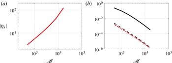Reference Carrier, Wu and Yeh2003), which is an indicator of wave breaking. It was, however, remarked by Synolakis (Reference Synolakis1987), who conducted laboratory experiments on solitary waves, that the post-breaking analytical wave profile approximates the actual wave very well when wave breaking occurs very close to the shoreline. The fact that we obtain a very good match in table 1 for the original case a of Carrier et al. (Reference Carrier, Wu and Yeh2003) suggests that numerical simulations may continue to predict accurate wave shape despite having waves breaking at the shoreline. This is of course permitted by the fact that we moved the first grid point away from the line of vanishing depth. We would like to point out that in our direct simulation of the governing equation (2.16) for case a the wave steepness, which is given by

grows unbounded as we decrease the grid size (figure 1 a), i.e. wave steepness at the shoreline does not converge. This is not unexpected since the Jacobian of the hodograph transformation in this case vanishes at the shoreline as discussed before. The runup itself, however, converges to the true runup value. For case  $\mathbf{a}^{\prime }$ , i.e. with decreased wave amplitude, the Jacobian does not vanish. Correspondingly, in our simulations, both the maximum runup value and wave steepness converge asymptotically (cf. figure 1 b).

Figure 1.

(a) Absolute value of the maximum wave steepness at the shoreline as a function of the number of grid points $\mathscr{M}$ for case a reported in table 1. Clearly in this case $|{\it\eta}_{x}|$ grows exponentially with $\mathscr{M}$ and does not converge. (b) The relative error of the maximum wave runup $e_{R}$ (dashed line), and the relative error of the maximum wave steepness $e_{{\it\eta}_{x}}$ (solid line) at the shoreline are shown as functions of $\mathscr{M}$ for the numerical simulation of case $\mathbf{a}^{\prime }$ reported in table 1. These relative errors are defined with respect to the values obtained for $\mathscr{M}=2^{15}$ (i.e. the finest grid simulated). The relative error of the maximum wave runup for case a (— ⋅ —) is also shown in this plot.

In the following section (§ 4) we study the evolution of landslide tsunamis in a lake, and present examples that highlight the effect of nonlinearities and wave reflections and interactions in the inundation maps that are specific to lakes and enclosed bodies of water.

4.1. The setup

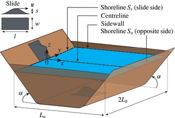
Let us focus our attention on a geometrically simple lake to highlight some of the physics involved. Specifically, we consider a shallow lake of rectangular surface area $L_{a}\times 2L_{b}$ confined symmetrically by two opposing vertical walls along $y=\pm L_{b}$ and two opposing sloping beaches aligned with the $\pm x$ direction (figure 2). A vertical wall may be an idealization of a mountain cliff or a dam. We assume that the two opposing beaches have the same slopes, and that they each occupy  $1/3$ of the horizontal extent of the lake. The remaining middle  $1/3$ is flat with the dimensionless depth of unity; therefore the beach slope is $\tan {\it\alpha}=3/L_{a}$ in the dimensionless space and ${\it\mu}\tan {\it\alpha}$ in the physical domain (note that in the dimensionless space vertical and horizontal lengths are scaled differently, cf. (2.6a, b )). The bottom is therefore given by

To avoid sharp corners an arc of radius $1/20$ (in dimensionless variables) connects each sloping beach to the flat bottom.

Figure 2.

Schematic of the lake and the landslide. The landslide is shown at both its initial position (above water) and its final position (underwater).

We consider the motion of a landslide whose height is given by

which describes a smooth and rigid hump-like landslide with a horizontally projected surface area of length  $l$ , width $w$ and maximum thickness $s$ that moves along the lake centreline (figure 2). The total water depth is therefore $h(x,y,t)=h_{0}(x,y)+h_{s}(x,y,t)$ . Physically speaking, (4.2) corresponds to a slide moving with a constant speed $v\sqrt{1+\tan ^{2}{\it\alpha}}$ down the beach. When the centre of the slide reaches the beach toe at $x=L_{a}/3$ , it decelerates according to a smooth cubic law $v\propto t^{3}$ until it reaches the middle of the lake where it stops (i.e. at $x=L_{a}/2$ , cf. figure 2).

Two types of waves are generated by the three-dimensional subaerial landslide as it enters the water. We refer to waves that propagate freely across the lake as outgoing waves, and to waves that are trapped by the shoreline as edge waves. Outgoing waves along open coasts, forced impulsively by landslides, have been the subject of a large number of laboratory experiments conducted for both solid landslides (e.g. Kamphuis & Bowering Reference Kamphuis and Bowering1970; Walder Reference Walder, Watts, Sorensen and Janssen2003; Panizzo, De Girolamo & Petaccia Reference Panizzo, De Girolamo and Petaccia2005a ; Panizzo et al. Reference Panizzo, De Girolamo, Di Risio, Maistri and Petaccia2005b ; Heller et al. Reference Heller, Moalemi, Kinnear and Adams2012) and granular landslides (Fritz, Hager & Minor Reference Fritz, Hager and Minor2004; Ataie-Ashtiani & Nik-Khah Reference Ataie-Ashtiani and Nik-Khah2008; Di Risio, De Girolamo & Beltrami Reference Di Risio, De Girolamo, Beltrami and Marner2011). More recently, properties of landslide-generated edge waves have also been investigated (e.g. Liu et al. Reference Liu, Wu, Raichlen, Synolakis and Borrero2005; Lynett & Liu Reference Lynett and Liu2005; Sammarco & Renzi Reference Sammarco and Renzi2008; Di Risio et al. Reference Di Risio, De Girolamo, Bellotti, Panizzo, Aristodemo, Molfetta and Petrillo2009). The following analysis of landslide tsunamis in lakes highlights the importance of nonlinearity as well as the significance of the interactions between outgoing and edge waves in the generation of unexpectedly large runups.

4.2. Numerical results and discussion

We choose the lake dimensions $L_{a}=1$ , $L_{b}=1.02$ and normalized slopes of $\tan {\it\alpha}=3$ . A solid mass of $w=l=0.25$ with thickness $s=0.07$ according to (4.2) slides down the beach $S_{s}$ with a horizontal speed $v=0.12$ (this specific set of parameters is chosen as it further highlights the physics to be discussed). A detailed sensitivity analysis is provided later. Simulation parameters are chosen to be ${\it\delta}a=0.002$ , ${\it\delta}b=0.002$ , with Courant number equal to 0.5 such that ${\it\delta}t=0.001$ , for which our simulations converge.

Figure 3.

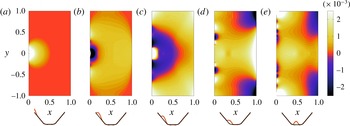
Snapshots of nonlinear dimensionless free-surface height $Z$ at (a)  $t=0.83$ , (b)  $t=1.66$ , (c)  $t=2.47$ , (d)  $t=3.76$ , (e)  $t=5.63$ . Physical parameters associated with the lake dimensions and slide shape are $s=0.07$ , $v=0.12$ , $L_{b}=1.02$ , $w=l=0.25$ , $\tan {\it\alpha}=3$ . Simulation parameters are ${\it\delta}a=0.002$ , ${\it\delta}b=0.002$ , ${\it\delta}t=0.001$ . The position of the slide with respect to the lake geometry is shown below each plot (slide height is magnified by a factor of four).

Snapshots of the water surface are shown in figure 3(a–e). Lighter colours show higher elevations and darker colours show depressions. Upon water entry at $t=0$ the land mass pushes the water forward, generating a big hump of water at its front (figure 3 a). This first hump then disintegrates into a radially spreading outgoing wave and a series of shoreline-trapped edge waves on the slide side  $S_{s}$ . A pair of edge-wave crests can be seen in figure 3(b) travelling away from the centreline $y=0$ . The outgoing wave crosses the length of the lake and reaches the opposite shoreline $S_{o}$ (figure 3 b), while a ring of depression is formed near the origin on the $S_{s}$ shore. Moments later (figure 3 c), the first outgoing and edge waves reach the corners of the lake ( $y=\pm L_{b}$ ) while a second hump is formed at the origin. Figure 3(d) shows the runup of the second outgoing wave on  $S_{o}$ , and the propagation of the edge waves resulting from the disintegration of the rebound hump along  $S_{s}$ . The leading edge wave of this second hump is the longest and largest in amplitude, as seen in white at $y\sim 0.63$ in figure 3(d). Finally, figure 3(e) shows the return of the second outgoing wave (the one initiated on $S_{s}$ in figure 3 c) to $S_{s}$ after reflection from  $S_{o}$ . This reflected wave superimposes on the trail of edge waves on  $S_{s}$ , resulting in higher runups at some locations along  $S_{s}$ , as will be elaborated shortly.

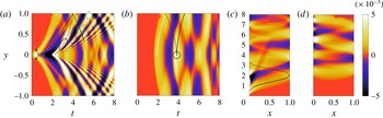
The time history of the water surface evolution along the shoreline $S_{s}$ ( $x=0$ ) is shown in figure 4(a), the shoreline $S_{o}$ ( $x=L_{a}$ ) in 4(b), the centreline of the lake ( $y=0$ ) in 4(c), and the vertical sidewalls ( $y=\pm L_{b}$ ) in 4(d). The first runup due to the water entry of the landslide is seen in figure 4(a) at $y=0,t\sim 0.5$ . It is then followed by a rundown that starts at $t\sim 1.4$ . From figure 4(a) it is seen that the dispersion of edge waves along $S_{s}$ is similar to that resulting from an initial hump in open water: longer waves travel faster and more crests are generated as time goes by (cf. Sammarco & Renzi Reference Sammarco and Renzi2008). Due to dispersion, edge waves elongate and accelerate as they travel away from the origin (cf. Sammarco & Renzi Reference Sammarco and Renzi2008; Mei, Stiassnie & Yue Reference Mei, Stiassnie and Yue2005), as can be seen from the convex shape of the edge-wave pathlines in figure 4(a) (marked by solid and dashed lines).

Figure 4(a) also shows the reflection of edge waves by the vertical sidewalls (i.e.  $y=\pm L_{b}$ ). The second edge wave due to the first runup (solid line) meets the leading edge wave due to the second runup (dashed line) when reaching the sidewall at $y=L_{b},t\sim 4.1$ . It then bounces back to interact with the other forward moving (i.e.  $+y$ direction) edge waves of the second hump (marked by dash-dotted lines). A relatively high runup at $y\sim 0.61,t\sim 4.8$ (highlighted by a circle) is partially due to this encounter.

The radially outgoing wave first reaches the opposite shoreline $S_{o}$ at $y=0,t\sim 1.7$ (figure 4 b). Wave runup patterns along $S_{o}$ (solid white and black lines) are arc-shaped due to radial spreading. The leading crest (marked by the white line) is reflected from the sidewall $y=L_{b}$ near $S_{o}$ at $t\sim 2.7$ and turns into an edge wave whose path is marked by a black dashed line. This edge wave advances toward the centre, and interacts with the second runup (marked by a black solid line) at $t\sim 3.7$ , resulting in a constructive interference (as marked by a circle). These interactions continue along $S_{o}$ as more edge/outgoing waves come into play. Contrary to edge waves, outgoing waves are non-dispersive. Therefore, as seen in figure 4(c), the depression and elevation rays appear straight where the water depth is constant (i.e.  $1/3\leqslant x\leqslant 2/3$ ), and curved near the shorelines because of refraction. The superposition of the leading edge wave of the rebound (second) runup on  $S_{s}$ with the reflected first outgoing wave (marked by a dashed line in figure 4 c), can be clearly seen in figure 4(a). The bright white spot resulting from this interaction is highlighted by an ellipse at $t\sim 3.3$ . Figure 4(c) shows that the two outgoing crests (from the first and the second runups) remain separated for the rest of the simulations, and that the amplitude of the first outgoing wave is smaller than the second one. Figure 4(d) shows the surface elevation along the vertical sidewalls. Both edge waves and outgoing waves emanating from the first runup reach the sidewalls at approximately $t\sim 2.7$ . They generate an almost horizontal beam across each of the two vertical walls. Edge waves on $S_{s}$ ( $x=0$ ) are also seen in figure 4(d) with their crests at $t\sim 4,5.5,7.5$ , and on $S_{o}$ ( $x=L_{a}$ ) at $t\sim 4.5,6.5$ .

Figure 4.

Time history of the nonlinear wave runup on (a) shoreline $S_{s}$ , (b) shoreline $S_{o}$ , and wave height along (c) centreline, (d) sidewall, for a landslide tsunami with physical and simulation parameters given in figure 3. The colour map shows the dimensionless free-surface height  $Z$ .

The multiple interactions between reflected outgoing waves and edge waves that occur in a lake suggest that extreme inundations may take place far away from the immediate neighbourhood of the landslide and some time after its submergence. As an example, in our simulation, an extremely large runup occurs at the lake corners ( $x=0,y=\pm L_{b}$ ) due to constructive interference between the third edge wave of the initial runup, the second edge wave of the rebound (second) runup, and the reflected second outgoing wave. 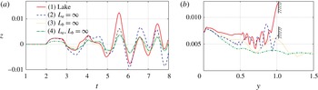This runup takes place at $t=5.5$ and is almost twice as big as any other runup along $S_{s}$ (seen as a bright-coloured region in figure 4(a) marked by a diamond). This runup is also much larger than that estimated by an open-coast calculation, as can be seen in figure 5(a) where we show the wave runup at $x=0,y=1.02$ as a function of time due to the same slide entering four different geometric configurations: (1) a lake of finite size ( $L_{a}=1,L_{b}=1.02$ , solid line), (2) an infinitely long lake ( $L_{a}\rightarrow \infty$ , dashed line), (3) an infinitely wide lake ( $L_{b}\rightarrow \infty$ , dotted line), and (4) an open coast ( $L_{a},L_{b}\rightarrow \infty$ , dash-dotted line). As expected, the runup is greatest for the finite-sized lake due to the presence of a wall at $y=L_{b}=1.02$ and an opposite beach at $x=L_{a}=1$ . The maximum runup for the case of an infinitely long lake, infinitely wide lake and an open coast is respectively 48 %, 54 % and 71 % lower than that of the finite size lake considered here.

Figure 5.

(a) Time history of nonlinear wave runup height at $y=1.02$ on $S_{s}$ for a slide entering: (1) a finite rectangular lake ( $L_{a}=1$ , $L_{b}=1.02$ ), (2) a long and narrow lake ( $L_{a}=\infty$ , $L_{b}=1.02$ ), (3) a short and wide lake ( $L_{a}=1$ , $L_{b}=\infty$ ), (4) an open coast ( $L_{a}=\infty$ , $L_{b}=\infty$ ). (b) Inundation maps up to $t=8$ along $S_{s}$ for $y\geqslant 0$ for the four cases displayed in (a). Physical and simulation parameters other than $L_{a}$ and $L_{b}$ are the same as in figure 3.

The inundation map of shore $S_{s}$ ( $y\geqslant 0$ ) for the four geometries considered above shows (figure 5 b) that the average runup increases in the presence of a wall and an opposite beach. For the open coast (dash-dotted line), edge waves result in a large runup less than a quarter of the slide width away from the centreline, i.e. very close to the origin. Edge waves amplitude then decreases as they propagate farther away (which is in qualitative agreements with earlier studies by Lynett & Liu Reference Lynett and Liu2005; Sammarco & Renzi Reference Sammarco and Renzi2008; Di Risio et al. Reference Di Risio, De Girolamo, Bellotti, Panizzo, Aristodemo, Molfetta and Petrillo2009). The contrast between the four cases studied here shows the importance of wave reflection from side/opposite boundaries and superposition in the magnitude and location of the maximum runup.

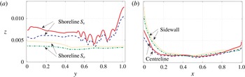
Of practical interest is also the importance of nonlinearities in the simulation presented. The inundation maps of the two shorelines $S_{s}$ and $S_{o}$ , as well as the maps of maximum wave height along the lake centreline and sidewalls, can be used to measure the significance of nonlinearity in the runup predictions. Figure 6(a) compares the linear versus nonlinear runup on both $S_{s}$ and $S_{o}$ . The maximum inundation predicted by the nonlinear theory is higher than the linear prediction everywhere on both $S_{s}$ and $S_{o}$ . In particular, the relative increase due to nonlinear effects at $y\sim 0.05$ on $S_{s}$ is ${\sim}50\,\%$ . Details of inundation curves can be better understood in the light of figure 4. For instance, the six local maxima between $y=0.55$ and $y=0.9$ on $S_{s}$ shown in figure 6(a) are partially due to the reflections by the sidewall at $y=L_{b}$ of the third and fourth edge waves of the rebound runup interacting with trailing edge waves at $t\sim 7$ . The extreme corner runup is found to be 20 % higher with nonlinear effects taken into account.

On the opposite shore $S_{o}$ , the runup of the second outgoing wave is responsible for most of the inundation for $y<0.5$ and is about 30 % higher when nonlinear terms are taken into account. The effects of wave shoaling and radial spreading are clearly seen in figure 6(b) by the rapid decrease of maximum wave height along the centreline away from the shorelines. Clearly, the quantitative difference between linear and nonlinear inundations is maximum closer to the shoreline since, due to nonlinear effects, larger wave height and steepnesses both contribute to a larger runup (cf. Didenkulova et al. Reference Didenkulova, Pelinovsky, Soomere, Zahibo and Kundu2007a ).

Figure 6.

Inundation maps of the (a) shorelines $S_{s}$ , $S_{o}$ (for $y\geqslant 0$ ), and (b) sidewalls and centreline as predicted by nonlinear (——, $\cdots \cdots$ ) and linear theories (– – –, — ⋅ —). Physical and simulation parameters are the same as in figure 3. Simulation are performed from $t=0$ to $t=8$ beyond which no further significant changes occur.

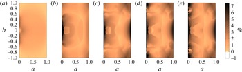
To investigate at what time stage during the landslide event major nonlinear effects come into play and where they are highlighted, we compare the maximum linear and nonlinear wave heights for all surface fluid particles (i.e. all pairs (a, b)) at five different times (figure 7 a–e). To quantify this difference between nonlinear and linear predictions we define

where $Z_{NL}$ ( $Z_{L}$ ) is the maximum nonlinear (linear) wave height for each pair ( $a,b$ ) and time $t$ , and $Z_{L,max}=\max \left[Z_{L}(t=t_{f}\rightarrow \infty )\right]$ is a single number that shows the overall maximum wave height as predicted by the linear theory. In our simulations the final time $t_{f}=8$ is chosen as $Z_{L,max}$ no longer changes for $t>t_{f}$ . Stronger differences (in %) are shown with darker colours. Note that the linear results are based on (2.20).

Nonlinearity comes, as is expected, from wave–bottom interactions near the line of vanishing depth (i.e. near the shoreline). Yet the first runup on $S_{s}$ , which is due to the slide starting to push the water, is only weakly nonlinear (as seen in figure 7 a). Therefore, major nonlinearities come into play when the rebound hump is formed and disintegrates into edge waves and outgoing waves (see dark patch localized near $S_{s}$ in figure 7 b). Physically speaking, this is due to the rundown being amplified by a downward dragging imposed by the landslide descending further under the water. Excess of wave height predicted by nonlinear terms is then seen almost everywhere in the lake as edge waves and outgoing waves reach the opposite shoreline and sidewalls (figure 7 c,d). Finally, figure 7(e) shows the contrast between maxima of nonlinear and linear predictions from $t=0$ to the final time $t_{f}=8$ . As discussed before, nonlinearity is much stronger near the shorelines and at the corners of the lake.

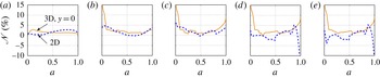
We remark that the strong contrast between nonlinear and linear predictions is partly due to the three-dimensional nature of the landslide-generated waves. To demonstrate this, we compare in figure 8 nonlinear and linear maximum wave heights along the lake centreline (i.e.  $\mathscr{N}(a,0,t)$ ) for the finite-width slide (i.e.  $w<L_{b}$ ; solid line) of the case studied in figures 3–7, and an infinitely wide landslide (i.e.  $w\rightarrow \infty$ ; dashed line), which makes the waves two-dimensional. As discussed before, the large nonlinearity $\mathscr{N}$ near $a=0$ for the three-dimensional case in figure 8(b) appears with the second runup $(\mathscr{N}(a,0,1.6)=16\,\%)$ . The much smaller difference in the two-dimensional case $(\mathscr{N}(a,0,1.6)=5\,\%)$ thus suggests that this increase is due to three-dimensional effects. Note that $\mathscr{N}$ is even larger than 16 % in the three-dimensional case just slightly away from the centreline ( $\mathscr{N}(a,0.05,1.6)=28\,\%$ , cf. figure 6). Another interesting behaviour specific to the two-dimensional case is that the linear theory overpredicts the maximum wave height sometime after the slide submergence (figure 8 d,e near the opposite shoreline). Note that the absolute value of $Z_{L,max}$ in the two-dimensional case can be much larger (about four times in the presented case) than its three-dimensional counterpart which is due to energy spreading in the three-dimensional case.

Figure 7.

Spatial distribution of the difference between nonlinear and linear maximum wave heights ( $\mathscr{N}$ , cf. (4.3)) during a landslide tsunami in a lake. (a–e) show the difference during time periods lasting from zero to $t_{f}=1.64$  (a), 3.30 (b), 4.97 (c), 6.63 (d), 8.00 (e). During the entire event, nonlinear wave-height predictions are higher than the linear ones, and the difference is higher close to the shorelines (cf. figure 6). Physical and simulation parameters are the same as in figure 3.

Figure 8.

Effect of the slide width on the difference between nonlinear and linear maximum wave heights along the lake centreline. The predictions are plotted for a finite width landslide ( $w<L_{b}$ , ——) and an infinitely wide landslide ( $w\rightarrow \infty$ , – – –). In the latter case the problem is two-dimensional, and therefore this figure also highlights effects of three-dimensionality on the significance of nonlinearity. (a)–(e) The difference ( $\mathscr{N}$ , cf. (4.3)) for time periods from zero to $t_{f}=1.64$ , 3.30, 4.97, 6.63, 8.00 (i.e. same as in figure 7), respectively. Note that $\mathscr{N}$ is much higher for the three-dimensional case, and that $\mathscr{N}$ becomes negative at some time in the two-dimensional case. Physical parameters (other than  $w$ ) and simulation parameters are the same as in figure 3.

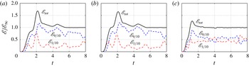
It is of interest also to assess how the energy ceded by the slide to the fluid is divided between edge waves and outgoing waves. For this purpose, in figure 9 we plot the total energy in the lake (solid line), the total energy very close to the shoreline $S_{s}$ in the area $0\leqslant a\leqslant 1/10$ (dash-dotted lines), and the total energy in the rest of the lake, i.e. in the area $1/10\leqslant a\leqslant 1$ (dashed line). The total energy is calculated via (2.25) and normalized by the total wave energy in the steady state when $t\rightarrow \infty$ (here $t=8$ ). The plot in figure 9(a) is with the same parameters as in figure 3. For comparison, we also show the spatial energy division for a smaller slide $s=0.07/2$ that moves: (i) at the original speed $v=0.12$ (figure 9 b), and (ii) twice as fast (i.e.  $v=0.24$ , figure 9 c). In all three cases (the first two being qualitatively very much alike) there is an overshoot of the total energy. This is because the initial outgoing wave has time to reflect on $S_{o}$ back to $S_{s}$ while the slide is still moving forward and opposes the motion of the reflected wave. The total energy reaches its steady-state value when the slide stops moving, i.e. at $t=6$ for the two slow slide cases and $t=3$ for the faster slide.

Comparison of figures 9(a,b) and 9(b,c) shows that the slide thickness does not have a major effect on the energy distribution while slide velocity does. For the slow landslide (figure 9 a,b) more energy is given to the outgoing waves and less energy is trapped, while for the fast slide the energy partitioning is almost even (figure 9 c). In figure 9(b), the first two humps of nearshore energy at $t\sim 0.9$ , 1.9 correspond to the generation of the first and second outgoing waves whereas the last three are associated with the return to $S_{s}$ of: (i) the first outgoing wave at $t=3.3$ and (ii) the second outgoing wave at $t=5.4$ and 7.7.

Figure 9.

Wave energy in the lake ( $\mathscr{E}$ , cf. (2.25)) normalized by steady-state wave energy ( $\mathscr{E}_{\infty }$ ) is shown for a landslide with: (a)  $s=0.07$ , $v=0.12$ ( $\mathscr{E}_{\infty }=0.967\times 10^{-6}$ ); (b)  $s=0.035$ , $v=0.12$ ( $\mathscr{E}_{\infty }=0.229\times 10^{-6}$ ); (c)  $s=0.035$ , $v=0.24$ ( $\mathscr{E}_{\infty }=2.220\times 10^{-6}$ ). The total wave energy in the lake (——) is divided to energy in the near- $S_{s}$ area ( $0<a<L_{a}/10$ , — ⋅ —); and the rest of the lake ( $L_{a}/10<a<L_{a}$ , – – –). Other physical and simulation parameters are given in figure 3.

Figure 10.

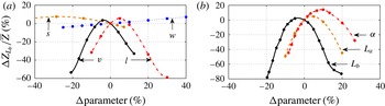
Sensitivity of the ratio of the maximum corner runup (normalized by the mean maximum runup) on $S_{s}$ $(Z_{L_{b}}/\overline{Z})$ to changes in (a) the landslide parameters ( $s,w,l,v$ ) and (b) the lake geometry parameters ( $L_{a},L_{b},{\it\alpha}$ ). The changes in the parameters are given in per cent and are measured relatively to those used for the reference lake and landslide studied in § 4.2 (i.e. figures 3–7). The other physical and simulation parameters are the same as in figure 3.

In order to investigate the sensitivity of the presented results to the lake and landslide parameters, we study the effect of the lake dimensions ( $L_{a},L_{b},{\it\alpha}$ ) and slide parameters ( $s,w,l,v$ ) on the importance of the corner runup, measured as the ratio of maximum corner runup to the average runup on $S_{s}$ , i.e.  $Z_{L_{b}}/\overline{Z}$ in which $\overline{Z}=(1/L_{b})\int _{0}^{L_{b}}Z(a=0,b,c=0)\,\text{d}b$ . Changes in the parameters and variables are measured relatively to the reference case studied in § 4.2 (i.e. figures 3–7). The relative importance of the corner runup, displayed in figure 10, is clearly very sensitive to the lake geometry (figure 10 b). For example, a 20 % decrease in the lake width leads to an 80 % drop in the relative corner runup. Figure 10(b) therefore further highlights that a change in the lake geometry affects the location and time of positive and negative interference of edge and outgoing waves. The importance of the corner runup is also significantly altered by the length and the velocity of the landslide but is almost independent of the thickness and width of the slide (figure 10 a). This suggests that uncertainties in the solid landslide length or speed are likely to result in unreliable maximum wave runup predictions.

We would like to finally comment on bottom friction, i.e. on the fact that long waves lose energy due to viscous effects near the seabed (cf. Bernatskiy & Nosov Reference Bernatskiy and Nosov2012; Geist, Lynett & Chaytor Reference Geist, Lynett and Chaytor2009). One way to model bottom friction is to introduce a friction term to the right-hand side of (2.10). A number of different forms of such a dissipation term can be found in the literature that, generally, involve one or more free parameters that can be adjusted for model calibration (e.g. Satake Reference Satake1995; Synolakis et al. Reference Synolakis, Bernard, Titov, Kânoğlu and González2008; Zelt & Raichlen Reference Zelt and Raichlen1990). For example, the dissipation term suggested by Zelt (Reference Zelt1991) reads in two dimensions

With $K=5\times 10^{-5}$ and ${\it\mu}\tan {\it\alpha}=3/60$ , Zelt & Raichlen (Reference Zelt and Raichlen1990) showed that their numerical results compared well with the physical experiments of Synolakis (Reference Synolakis1987) on non-breaking solitary waves running up a $1/20$ sloping beach. With the inclusion of this friction term into our model, we obtained less than 2 % maximum runup deviations from the runup values presented in figure 6. This indicates that dissipation by bottom friction can be safely neglected for the results presented here.