Implications
The body composition and body part masses were predicted for a wide range of live weights, that is, from 3 to 100 kg, of dairy goat wethers of the Saanen and Swiss Alpine breeds. In the absence of specific estimates in the literature, the results of this study might be useful for predicting the protein and energy requirements for bucklings and doelings, specifically until the age at first mating in the latter category. In addition, the allometric equations estimated here are useful for predicting other traits such as dressing percentage and the weights of the organs, other body parts, and fresh gut contents.
Introduction
Huxley and Teissier (Reference Huxley and Teissier1936) coined the term allometry to describe the growth of body parts relative to a standard or the body proper and employed the following equation to describe, in their words, ‘the elementary law of relative growth or law of simple allometry’:
 $$\mu _{{Y_{t} }} \,{\equals}\,\,\alpha X_{t}^{\beta } $$
In this equation,
 $\mu _{{Y_{t} }} $
is the expected mean of a variable Y
t
, measured as a body part or chemical constituent at a given time (t), and the body mass (BM), or another standard such as the empty body mass (EBM), simultaneously measured with Y
t
, is ascribed to X
t
. Assuming an exponential growth for both Y
t
and X
t
, the parameters α and β aggregate both the intercepts at t=0 and the first-order, specific growth rates k
2 and k
1 (both expressed as 1/t) for Y
t
and X
t
, respectively. Therefore,
 $\alpha \,{\equals}\,Y_{{\rm 0}} /X_{0}^{{k_{2} /k_{1} }} $
(expressed as, e.g., g or
 ${\rm MJ}/{\rm kg}^{{k_{2} /k_{1} }} $
) and the dimensionless scaling exponent β=k
2/k
1. Because k
2 can be ⩾ or ⩽k1, a given allometric trend can be positive (β>1), negative (β<1) or isometric when β=1 (Brody, Reference Brody1945). This model has been used to study size effects over several body traits to quantify proportional changes, make practical predictions, and for inter- and intraspecific comparisons because of its mathematical simplicity and its reliance on the dominant effect of BM on many evolutionary, ecological, morphological, physiological and productive traits (Huxley and Teissier, Reference Huxley and Teissier1936; Brody, Reference Brody1945; Gould, Reference Gould1966; Kleiber, Reference Kleiber1975; Glazier, Reference Glazier2013; Packard, Reference Packard2013). It is also useful for describing the ontogenetic growth as the quantitative analysis of allometric trends among growth stages within a species, breed, or productive type (Brody, Reference Brody1945; Gould, Reference Gould1966; Packard et al., Reference Packard, Birchard and Boardman2011). Traditionally, ordinary least squares (OLS) regression on log-log transformation have been applied to fit equation (1) in bivariate allometry, in spite of the open debate between OLS log-log fitting advocates v. those who are in favor of nonlinear parameter estimation in the arithmetic scale (Hui and Jackson, Reference Hui and Jackson2007; Glazier, Reference Glazier2013; Packard, Reference Packard2013; Mascaro et al., Reference Mascaro, Litton, Hughes, Uowolo and Schnitzer2014). This issue makes relevant the diagnostics of models fitted under different assumptions, fitting procedures, and by a multimodel inference approach (Burnham and Anderson, Reference Burnham and Anderson2004; Vonesh, Reference Vonesh2012), which matters for the accuracy and precision of parameter estimates and predictions.
The ontogenetic growth of morphological and physiological traits with respect to BM have been studied in goats to predict carcass and non-carcass components, yields of commercial cuts, bones, muscle, fat and for quantifying the chemical composition of the body to predict nutrient requirements. There is concordance about some reported ontogenetic trends in domestic goats, such as the positive allometry for internal fat deposits and total fat amounts, negative allometry for body water amount and fasting heat production, and inconsistent patterns for protein retention (Colomer-Rocher et al., Reference Colomer-Rocher, Kirton, Mercer and Duganzich1992; Luo et al., Reference Luo, Goetsch, Nsahlai, Johnson, Sahlu, Moore, Ferrell, Galyean and Owens2004; Yáñez et al., Reference Yáñez, Resende, Ferreira, Pereira Filho, Medeiros and Teixeira2009; Almeida et al., Reference Almeida, Resende, Silva, Soares, Fernandes and Teixeira2015). However, intraspecific comparisons require a wider and balanced range of BMs (low leverage effect in the range) to demonstrate the dominant effect of size on parameter estimates of equation (1), including the variance, for a given trait (Packard, Reference Packard2013). Otherwise, variables that are generally ignored or neglected in the allometric analysis may influence the dependent variable and reduce the effect of BM over parameter estimates (Kleiber, Reference Kleiber1975). Araujo et al. (Reference Araujo, Vieira, Rocha, Abreu, Glória, Rohem Júnior and Fernandes2015) demonstrated that the scaling function fitted by nonlinear parameter estimation by maximum likelihood (ML), compared with ratios between growth models relating body parts to the whole body for dairy goat wethers (castrated male goats), better mimics the allometry of traits as functions of the BM or EBM based on information criteria. Nonetheless, Araujo et al. (Reference Araujo, Vieira, Rocha, Abreu, Glória, Rohem Júnior and Fernandes2015) did not address the ontogenetic growth of many body parts and the quality of fit of the equation (1) based on different assumptions regarding the type of probability density function (e.g. normal v. lognormal), and variance assumptions by consequence (e.g. homoscedasticity v. heteroscedasticity), associated to the dependent variable in bivariate allometry (Packard, Reference Packard2013; Mascaro et al., Reference Mascaro, Litton, Hughes, Uowolo and Schnitzer2014). Therefore, our objectives were to employ the equation (1) to obtain parameter estimates and predictions of body parts and chemical composition by using the BM and the EBM as individual predictors, and to evaluate traditional and alternative assumptions to fit the scaling function to mimic the ontogenetic growth profiles of dairy goat wethers.
Material and methods
The information used in this study was the raw data (n=58) from Araujo et al. (Reference Araujo, Vieira, Rocha, Abreu, Glória, Rohem Júnior and Fernandes2015), who investigated the growth of goat (Capra hircus, Linnaeus 1758) wethers of the Saanen and Swiss Alpine breeds, which exhibit a wide BM range (≅3 to 100 kg). The animals were slaughtered at birth and at 15, 90, 135, 210, 270, 365, 485, 610, 735, 790, 840, 890 and 920 days of age. The kids were castrated at 15 days old; they were weaned at 90 days old and were all fed ad libitum thenceforth. Approximately four to six animals were slaughtered per age, and the recorded variables were the masses of the head and members, carcass, blood, skin, heart, liver, reproductive tract, tongue and esophagus, lungs and trachea, spleen, pancreas, bladder, kidneys, gallbladder and the individual segments of the gastrointestinal tract (GIT): the ruminoreticulum, omasum, abomasum, small intestine and large intestine. By calculating the difference between the full and empty masses, we computed the fresh contents of each GIT segment and directly measured the internal fat mass as the sum of the masses of the omental, pelvic and renal fat deposits. Furthermore, we determined the masses of the trimmed cuts as the sum of the masses of the diaphragm, non-carcass muscle pieces and the thymus, and incorporated the recorded amounts of water, CP, crude fat, ash and total energy retained in the empty body. The details about the rearing of the goats from birth to maturity can be found in Araujo et al. (Reference Araujo, Vieira, Rocha, Abreu, Glória, Rohem Júnior and Fernandes2015).
Description of the quantitative relationships
We used equation (1) to describe the measured masses of the body parts (morphological traits) by considering X t =BM and the amounts of water, CP, crude fat, ash and energy in the empty body by considering X t =EBM. We excluded the masses of the ruminoreticulum and ruminoreticular contents for t=0 and 15 days of age to predict both the full and empty ruminoreticular masses because these values were negligible at smaller BM values, that is, for t⩽15 days old.
We first addressed the ontogenetic growth relationship by treating the fit of equation (1) to the bivariate Y
t
and X
t
data as a generalized nonlinear regression problem, by assuming that
 $$Y_{t} \sim {\rm Normal}\,( {\mu _{{Y_{t} }} {\rm ,}\,\sigma _{{Y_{t} }}^{2} } )$$
. Therefore, we fitted the model to the as measured data, that is in the arithmetic scale, as follows:
 $${\rm Y}_{t} \,{\equals}\,\mu _{{Y_{t} }} {\plus}e_{t} $$
This general nonlinear stochastic version completes the framework for describing the variables, in which e
t
 $\,\sim {\rm Normal}\,( {0, \,\sigma _{{Y_{t} }}^{2} } )$
and cov(e
t
,e
t')=0 as additional assumptions about the variance of the error term (e
t
). This formulation is general because we can ascribe several forms to the variance in Y
t
, namely
 $\sigma _{{Y_{t} }}^{2} $
, beyond the traditional homoscedastic assumption:
 $$\sigma _{{Y_{t} }}^{2} {\equals}\,\sigma ^{2} $$
 $$\sigma _{{{ Y}_{{ t}} }}^{2} \,{\equals}\,\sigma ^{2} \,{\rm exp}\left( {2\delta X_{t} } \right) \,\, \rm and $$
 $$\sigma _{{Y_{t} }}^{2} \,{\equals}\,\sigma ^{2} \left| {\mu _{{Y_{t} }} } \right|^{{2\psi }} $$
This formal statistical notation is useful because in these different forms, parameter σ
2 is the true random error variance, and equation (3) represents the traditional homoscedastic assumption. However, because scale may influences variability (Bard, Reference Bard1974; Vonesh, Reference Vonesh2012), we evaluated the exponential function using equation (4) for describing variances that varied exponentially with X
t
at a rate δ (with a reciprocal unit of X
t
), and evaluated equation (5) as the power-of-the-mean function for mimicking variances that scaled to the absolute expected mean,
 $\mu _{{Y_{t} }} $
. Both parametric values of δ and the dimensionless ψ belong to the interval (−∞, ∞).
The traditional log-log transformation using natural logarithms (log) was performed by assuming that
 $Y_{t} \sim {\rm Lognormal}\,( {\mu _{{Y_{{\rm t}} }} ,\, \sigma _{{Y_{{\rm t}} }}^{2} } )$
. A corollary of this assumption is that the expected mean (E[Y
t
]) in the arithmetic scale corresponds to the geometric mean of Y
t
, and the variance (V[Y
t
]) is actually a function of the expected geometric mean, as follows:
 $$E\left[ {Y_{t} } \right]\,{\equals}\,\mu _{{Y_{t} }} \,{\equals}\,{\rm exp}\left( {\mu {\plus}\sigma _{{\rm l}}^{2} /2} \right) \,\,\rm and $$
 $$V\left[ {Y_{t} } \right]\,{\equals}\,\sigma _{{Y_{t} }}^{2} \,{\equals}\,{\rm exp}\left( {2\mu {\plus}2\sigma _{{\rm l}}^{2} } \right){\minus}{\rm exp}\left( {2\mu {\plus}\sigma _{{\rm l}}^{2} } \right)$$
Because we assumed a probability density function (pdf) for Y
t
as lognormal, consequently, the logarithm of Yt follows a normal distribution as
 ${\rm logY}_{t} \sim {\rm Normal}\,\left( {\mu , \,\sigma _{{\rm l}}^{2} } \right)$
. Therefore:
 $$E\left[ {{\rm log}\,Y_{t} } \right]\,{\equals}\,\mu \,{\equals}\,{\rm log}\,\alpha {\plus}\beta \,{\rm log}\,X_{t} $$
To complete the stochastic version of equation (8) and to fit it in bivariate allometry, we have to add the error term:
 $${\rm log}\,Y_{t} \,{\equals}\,\mu {\plus}e$$
in which
 $e \sim {\rm Normal}\,\left( {0,\, \sigma _{{\rm l}}^{2} } \right)$
, and cov(e,e')=0. Another consequence to this traditional approach is that parameter α must be presented in the arithmetic scale as a geometric mean too, that is,
 $E\left[ \alpha \right]\,{\equals}\,\hat{\alpha }\,{\equals}\,{\rm exp}\,( {\widehat{{{\rm log}\,\alpha }}{\plus}\hat{\sigma }_{{ l}}^{2} /2} )$
. An important distinction must be made between parameters σ and σ
l
. The former is the standard deviation of the true error (residual) of Y
t
in the arithmetic scale by assuming
 $Y_{t} \sim {\rm Normal}\,( {\mu _{{Y_{t} }} ,\, \sigma _{{Y_{t} }}^{2} } )$
, whereas the latter is the residual standard deviation of logY
t
, and both μ, e and σ
l
are in the log scale.
The assumptions about variance functions to describe homoscedastic and heteroscedastic variations associated to the normal distributed Y t were combined with the scaling function to analyze the ontogenetic growth of the dairy goat wethers in the arithmetic scale. Therefore, we named the combination of equation (2) with the homogeneous variance function or equation (3) as MOD1. To evaluate the possible existence of heteroscedasticity, we combined equation (2) with equation (4), and equation (2) with equation (5) to yield MOD2 and MOD3, respectively. We named the traditional fit of Y t in the logarithmic scale, that is equations (6) to (9), as MOD4. The notation Θ r indicates the vector of parameters, and the number of parameters (p r ) used for predictions based on the rth models were p 1=p 4=3, and p 2=p 3=4.
Model fitting
The Newton–Raphson optimization algorithm (TECH=NEWRAP) implemented in the NLMIXED procedure (v. 9.4; SAS System Inc., Cary, NC, USA) minimized the negative logarithm of the likelihood function of the normal distribution following a parameter grid search (Vonesh, Reference Vonesh2012) for fitting MOD1, MOD2, and MOD3. In this framework, the minimization of the negative logarithm of the likelihood function implies the reciprocal maximization of the likelihood function of the normal distribution.
The fitting of MOD4 was a two-step process. First, we used the GLM procedure of SAS to fit equation (9) to log-log scale data by OLS. In sequence, the values of the estimated parameters were used as input parameter values in the NLMIXED procedure, but no optimization was allowed (TECH=NONE). In this way, we used NLMIXED to obtain predictions of Y t back-transformed into the arithmetic scale. The generalized log-likelihood function of the lognormal distribution was programmed in the NLMIXED procedure. The SAS programs for both normal and lognormal distributed variables are provided in the Appendix.
Evaluation of the quality of fit of the models
The models fitted by assuming
 $Y_{t} \sim {\rm Normal}\,( {\mu _{{Y_{t} }} ,\, \sigma _{{Y_{t} }}^{2} } )$
as MOD1, MOD2 and MOD3 have their log-likelihood function estimates directly comparable by the Akaike Information Criterion (AIC). Nevertheless, only those fitted models that converged and yielded positive definite Hessians for the variance–covariance matrix we regarded for multimodel inference. In sequence, the resultant valid fitted models were down-ranked according to their model probabilities (w
r
), which were calculated by computing the AIC adjusted for finite corrections, AICc
r
; the Akaike differences, Δ
r
; w
r
itself; and the evidence ratio (ER
r
) for each rth model in the set of three models, following the recommendations of Burnham and Anderson (Reference Burnham and Anderson2004).
The estimates of the log-likelihood function for MOD1, MOD2 and MOD3 are not comparable with the estimates of the log-likelihood obtained for MOD4, because their scales, and by consequence AICcr values, were in different dimensions. Therefore, we have to use the goodness-of-fit macro %GOF applicable to the NLMIXED procedure (Vonesh, Reference Vonesh2012). We used the average model adjusted concordance correlation (ρ C ) as a %GOF output to compare the four models. In addition, we computed the Z=tanh−1(ρ C ) transformation, which yields estimates with better asymptotic normality (Lin, Reference Lin1989). The criteria adopted was the closer the estimate of ρ C to one the better the model was, and the greater the Z transform value the better the model was.
Model predictions and parameter estimates
A fitted model evaluated according to multimodel inference that presented w
r
⩾0.90 was considered the best solution for describing a given variable because of the low level of uncertainty regarding its choice. For those models that yielded a high level of uncertainty during the selection process, for example, max w
r
<0.90, it was necessary to average the estimates of parameters and predictions. Thus, model averaging was performed for the valid fitted models whose down-ranked model probabilities amounted to
 $\mathop{\sum}\nolimits_{r\,{\equals}\,1}^R {w_{r} \ges\, 0.99} $
, and the w
r
values were rescaled in sequence as corrected model probabilities based on the selected models (R′), namely
 $w_{r}^{\prime} $
, so that
 $\mathop{\sum}\nolimits_{r\,{\equals}\,1}^{R^{\prime} } {w_{r}^{\prime} {\equals}1} $
. Therefore, for any parameter common to all model combinations (α, β, and σ) or any estimated general function of the parameters,
 $\hat{g}\left( {\hat{\iTheta }_{r} } \right)$
averaged as
 $\widehat{{\bar{g}}}$
, the following equations are true (Burnham and Anderson, Reference Burnham and Anderson2004):
 $$\widehat{{\bar{g}}}\,{\equals}\mathop{\sum}\limits_{r{\equals}1}^{R\prime} {w_{r}^{\prime} \ \hat{g}\left( {\hat{\iTheta }_{r} } \right)} \,\, \rm and $$
 $$\hat{V}\left[ {\widehat{{\bar{g}}}} \right]{\equals}\left( {\mathop{\sum}\limits_{r{\equals}1}^{R\prime} {w_{r}^{\prime} } \left( {\hat{V}\left( {\hat{g}\left( {\hat{\iTheta }_{r} } \right)} \right){\plus}\left( {\hat{g}\left( {\hat{\iTheta }_{r} } \right){\minus}\widehat{{\bar{g}}}} \right)^{2} } \right)^{{0.5}} } \right)^{2} $$
Equation (10) is the estimator of the averaged predictions or the average of the common parameter estimates (same dimensions and biological meaning, e.g.
 $$\widehat{{\bar{\alpha }}}$$
). Equation (11) is the estimator of the unconditional variance in the averaged predictions
 $( {\hat{V}[ {\widehat{{\bar{g}}}} ]} )$
, or the variance in the averaged parameter estimates (e.g.
 $\hat{V}[ {\widehat{{\bar{\alpha }}}} ]$
), which are based on the estimated variance of a given function of the parameters of the rth fitted model,
 $\hat{V}( {\hat{g}( {\hat{\iTheta }_{r} } )} )$
. Its squared root is the standard error of the prediction (or parameter estimate), an output of the NLMIXED procedure. The average standard error of
 $\widehat{{{ \bar{g}}}}$
is
 $\widehat{{{\rm SE}}}[ {\widehat{{\bar{g}}}} ]{\equals}( {\widehat{V}[ {\widehat{{\bar{g}}}} ]} )^{{0.5}} $
, which was used to build unconditional 99% confidence intervals (99% CI) based on the z-abscissa of the standard normal distribution as follows:
 $\widehat{{\bar{g}}}\,\pm\,2.58( {\widehat{{{\rm SE}}}[ {\widehat{{\bar{g}}}} ]} )$
. For those fitted models that presented w
r
⩾0.90, conditional 99% CI for all parameters were based on a t-distribution and the according degrees of freedom (df) (Vonesh, Reference Vonesh2012). The reader can determine any estimates for σ missing from the results by isolating the missing parameter in equation (10) and replacing it with known values, including the
 $w_{r}^{\prime} $
from the reported down-ranked w
r
values. We draw inferences about positive, negative, or isometric allometry based on confidence interval estimates for β.
For comparison purposes, the daily retentions of both EBM protein and energy were predicted for some BMs commonly reported in the literature (Colomer-Rocher et al., Reference Colomer-Rocher, Kirton, Mercer and Duganzich1992; Al-Owaimer et al., Reference Al-Owaimer, Suliman, El-Waziry, Metwally and Abouheif2013; Ferreira et al., Reference Ferreira, Yáñez, Medeiros, Resende, Pereira Filho, Fernandes, Almeida and Teixeira2015), namely 20, 27, 35 and 45 kg BM. In addition, these masses were references to predict protein and energy contents with reference to EBM and EBM0.75. These predictions were based on MOD1, MOD2 and MOD3 according to the multimodel selection framework. Because the first derivative of equation (1), that is
 ${\rm d}\mu _{{Y_{t} }} \,/\,{\rm d}X_{t} $
, is a general nonlinear function of the scaling function parameters given by:
 $$\hat{g}\left( {\hat{\iTheta }_{r} } \right)\,{\equals}\,\widehat{{\alpha \beta {\rm X}_{t}^{{\beta {\minus}1}} }}\,\, \rm or $$
 $$\hat{g}\left( {\hat{\iTheta }_{r} } \right)\,{\equals}\,\alpha \beta \widehat{{X_{t}^{{\beta {\minus}1}} }}X_{t}^{{0.25}} $$
for X t =EBM, equations (10) and (11) were both applied to obtain the according unconditional 99% CI. Alternatively, we estimated conditional 99% CI for those variables described by fitted models with an assumed high level of certainty, that is w r ⩾0.90. The dimensions of equations (12) and (13) are g/kg and g/kg0.75 for protein retention after multiplying by 1000 and MJ/kg and MJ/kg0.75 for energy retention, respectively.
We obtained some predictions regarding the traditional log-log approach and back-transformation via NLMIXED by assuming
 $Y_{t} \sim {\rm Lognormal}\,( {\mu _{{Y_{t} }} }} , \,\sigma _{{Y_{t} }}^{2} } )$
for comparisons with the other models. As mentioned before, we reported estimates for parameter α as its geometric mean, and predictions for
 $\mu _{{Y_{t} }} $
of equation (6) and
 $\sigma _{{Y_{t} }}^{2} $
of equation (7) as outputs of the NLMIXED procedure with no optimization allowed. In sequence, for graphical representations of MOD4, we built conditional 99% CI as
 $$\hat{\mu }_{{Y_{t} }} \,\pm\,t_{{0.01,\,{\rm df}}} ( {{{\hat{\sigma }_{{Y_{t} }}^{2} } \mathord{/ {\vphantom {{\hat{\sigma }_{{Y_{t} }}^{2} } {( {N{\minus}p_{4} } )}}} \kern-\nulldelimiterspace} {( {N{\minus}p_{4} } )}}} )^{{0.5}} $$
, with df computed accordingly. We also computed
 $Y_{t} {\minus}\hat{\mu }_{{Y_{t} }} $
as residuals in the arithmetic scale to illustrate some residual patterns for MOD4.
Results
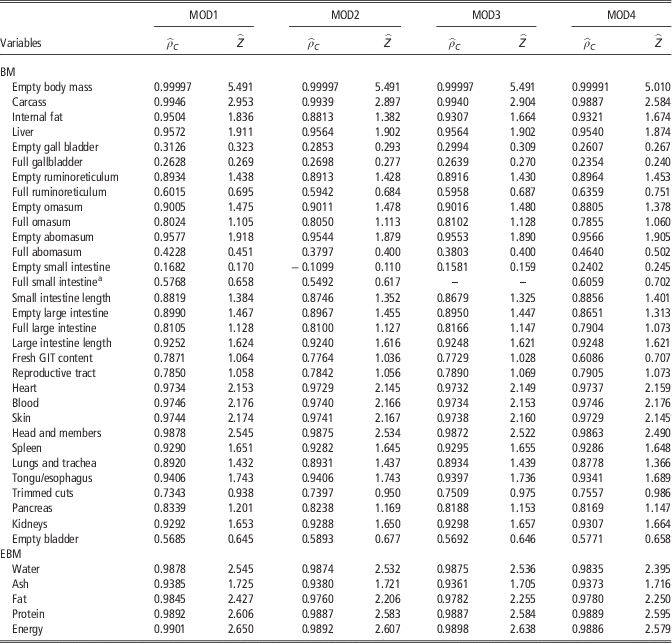
Combining equation (2) with the variance functions described by equations (3) to (5) as MOD1, MOD2 and MOD3 enabled the estimation of the relationships among the body parts and body composition scaled to both the BM and the EBM, respectively. The adopted criteria allowed the choice of the best models to represent the studied ontogenetic relationships. The chosen models explain the observed variability in the masses of the internal fat, empty and full gallbladder, full omasum, empty small intestine, blood, trimmed cuts and empty bladder as the body parts and the protein and fat quantities in the empty body (Table 1), and the choices were based on a low level of uncertainty (w r ⩾0.90). The MOD2 better described only two variables (w r ⩾0.90): internal fat and the empty small intestine. The homoscedastic assumption for MOD1 was unlikely given the data, and MOD3 was the best choice for eight (w r ⩾0.90) of the 36 traits studied (Table 1). For all of the other variables listed in Table 1, that is for 26 traits, a model averaging process was the best solution, because the level of uncertainty would be high (∀w r <0.90) if we took for granted only fitted models with the smallest AICcr as the best solution for each trait.
Computed information criteriaFootnote a of fitted models to ontogenetic allometry of dairy goat wethers

BM=body mass; EBM=empty body mass; GIT=gastrointestinal tract.
Standards were BM and EBM. Models are combinations of the scaling function with homoscedastic (MOD1), exponential (MOD2) or power-of-the-mean (MOD3) variance functions.
a AICc r is the Akaike information criterion corrected for small samples, Δ r is the Akaike difference, w r is the model probability and ER r is the evidence ratio computed for each rth model (r=1, 2, 3).
b The Hessian after convergence was not positive definite.
We evaluated MOD1, MOD2 and MOD3 based exclusively on information criteria. Nonetheless, because scales for estimates of the logarithm of the likelihood functions (normal v. lognormal) are different, and so AICcr values, we had to compute ρ C and Z as alternative measures for evaluating goodness-of-fit of MOD1 through MOD4. According to the chosen criterion regarding absolute estimates for ρ C and Z, the MOD4 was the best solution for 11 of the 36 traits studied (Table 2).
Estimates of the average model adjusted concordance correlation
 $\left( {\hat{\rho }_{C} } \right)$
and the respective
 $\hat{Z}{\minus}{\rm transform}$
for each fitted model

GIT=gastrointestinal tract.
Models are combinations of the scaling function with homoscedastic (MOD1), exponential (MOD2) or power-of-the-mean (MOD3) variance functions fitted by nonlinear parameter estimation, and MOD4 is the traditional log-log approach back-transformed to the arithmetic scale.
a The Hessian for MOD3 was not positive definite and the solution was discarded.
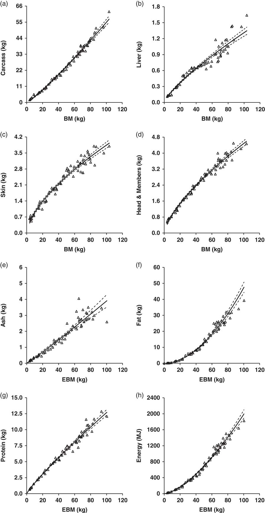
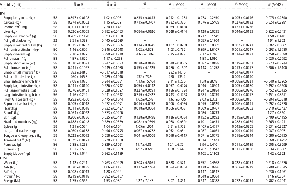
Parameter and averaged parameter estimates regarding the body parts, the EBM, carcass and internal fat exhibited positive allometric growths with respect to BM (β>1, Table 3), that is, faster specific growths compared with the growth of the body proper (Figure 1a). The liver, full gallbladder, full and empty ruminoreticulum and abomasum, full small intestine, full and empty large intestine, the length of the small and large intestines, the remaining reproductive tract, heart, blood, skin, head and members, lungs and trachea, tongue and esophagus, trimmed cuts, pancreas, kidneys, and empty bladder presented negative allometric trends (β<1, Table 3), meaning that these variables grew more slowly than the whole body (Figure 1b–d). The empty gallbladder, full and empty omasum and spleen presented isometric growths (β=1, Table 3). However, some significant estimates for β presented by some variables may not have practical importance in terms of relative growth, such as EBM (β>1, Table 3), because relative growth was practically linearly related with BM1 with a non-zero estimate for α. The result for the mass of the empty small intestine was unique because this variable was independent of the BM of the wethers (β=0, Table 3). In terms of EBM as a standard predictor of body chemicals, fat and energy exhibited positive allometric behaviors (β>1, Table 3, Figure 1f and h); ash presented isometric growth (β=1, Table 3 and Figure 1e); and the amounts of water and protein in the empty body presented negative allometric growth (β<1, Table 3, Figure 1g). The fresh GIT contents deviated from isometric growth (β<1, Table 3) and grew slower than the whole body. In addition, a large variability in the GIT contents was observed, particularly at smaller BM values, such as those of younglings (e.g. 100×1.621/0.953 ≅ 170%).
Solid lines are predictions ((f) and (g) are based on MOD3) or averaged predictions (panels (a), (b), (c), (d), (e) and (h)), and dashed lines cover the respective 99% confidence intervals for some observed traits (Δ) as functions of body mass (BM, (a) to (d)) and empty body mass (EBM, (e) to (h)) of dairy goat wethers.

Interval estimates for parameters of the ontogenetic growth of dairy goat wethers

GIT=gastrointestinal tract; n=sample size.
99% confidence intervals are unconditional for averaged estimates of common parameters based on multimodel selection
 $\widehat{{\bar{\alpha }}}$
, and are conditional for single parameter estimates
 $\hat{\alpha }$
for fitted models with high model probabilities (w
r
⩾0.90). The results refer to MOD1, MOD2 and MOD3.
a Variables described after selecting the best model as the one with w r ⩾0.90.
We only presented the parameter estimates of the best fits of MOD4 according to the highest
 $\hat{\rho }_{{ C}} $
, and consequently
 $\hat{Z}$
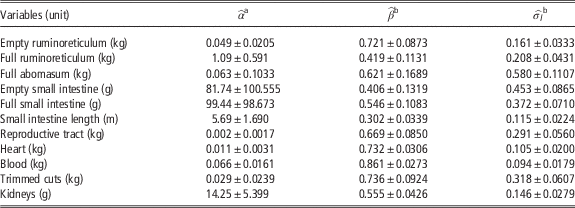
(Table 4). The estimates of the scaling exponent of the traits full abomasum, empty and full small intestine, and remaining reproductive tract presented discrepant results from those estimates of the model averaging process, whereas the remaining seven traits agreed in terms of β estimates based on their overlapping confidence intervals. As mentioned earlier, the estimates of the standard deviations are not comparable (Table 3
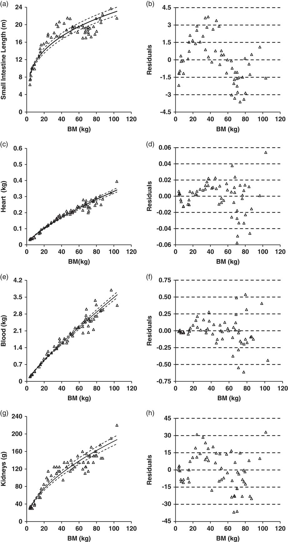
v. Table 4). The choice of MOD4 to mimic the ontogenetic growth was based on the assumption that residuals were heteroscedastic in the arithmetic scale, with an identifiable ‘right-oriented megaphone’ pattern, which departed from an ideal horizontal band over the BM range representing an unbiased homoscedasticity (Figure 2d and f). In addition, some variables presented sequences of residuals systematically occurring below and above the zero residual line (Figure 2b and h), but all traits interpreted with MOD4 chosen as the most suited solution presented negative allometry. The same residual pattern occurred even after the model averaging process, for example, Figure 1b (residual sequence not shown). MOD4 was also the best solution to describe one trait with an odd, unexpected behavior (not shown), that is, the mass of the empty small intestine. The fit of this model yielded a positive estimate for β (Table 4), whereas the fit of MOD2 yielded a negative point estimate not different from zero, which would had lead us to interpret as a case of non-scaling if we did not fit MOD4 (Table 3).
Observed (Δ), predicted (solid lines) and 99% confidence intervals (dashed lines) for some traits as functions of body mass (BM) in dairy goat wethers ((a), (c), (e) and (g)). Predictions are back-transformed into the arithmetic scale assuming lognormal distribution (MOD4). The respective residual sequences for each morphological trait are displayed on panels (b), (d), (f) and (h).

99% confidence interval estimates for parameters of MOD4

The results presented refer to those variables in which MOD4 was the best solution according to the average model adjusted concordance correlation.
a Back-transformed prediction into the arithmetic scale using the NLMIXED procedure.
b Point estimates obtained by ordinary least squares and interval estimates obtained using NLMIXED. The standard deviation of the error is in the logarithmic scale.
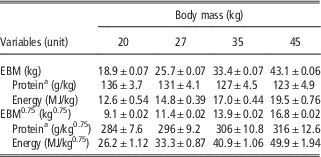
Unconditional 99% CI for EBM and the EBM retained energy, and conditional 99% CI for EBM protein were generated as predictions based on equations (12) and (13) as model averages for EBM and Energy, and based on the selected MOD3 for protein (Table 5). The energy retained per kg of empty body gain (MJ/kg) was not constant in the 20 to 45-kg BM interval. The amounts of protein and energy retained with EBM gain showed opposite responses, but both the protein and energy retained with the gain in EBM0.75 scale by the dairy goat wethers increased with BM (Table 5).
99% confidence intervals for empty body gain of protein and energy both scaled to one and 3/4 powers of the empty body mass (EBM) predicted at different body masses of dairy goat wethers

a Protein estimates are conditional. Other estimates are unconditional, averaged ones.
Discussion
The fitting process of the scaling function by nonlinear estimation methods yields a high absolute correlation among parameters β and α at convergence (Araujo et al., Reference Araujo, Vieira, Rocha, Abreu, Glória, Rohem Júnior and Fernandes2015). Gould (Reference Gould1966) recognized this problem of mathematical dependency and artifact correlation earlier. Because α is actually a function of β, which explains the high absolute correlation (not shown, but generally it was greater than 0.95 in our results), the estimates at convergence may always be biased to some unknown extent and dependent of the dataset. Therefore, the larger and more representative the data set, the greater the accuracy and precision of the estimates (Hui and Jackson, Reference Hui and Jackson2007).
The need to account for heterogeneous variances in the traits that were quantitatively interpreted from the scaling function appeared justified. The introduction of a weighting function to accommodate deviations from homoscedasticity for a given dependent variable as a function of the predictor X
t
, as in MOD2, or the expected
 $\mu _{{Y_{t} }} $
, as in MOD3, removes scale effects generated by the independent variable (BM or EBM here) from the residual variance (Bard, Reference Bard1974; Hui and Jackson, Reference Hui and Jackson2007; Vonesh, Reference Vonesh2012). In our study, heterogeneous variance functions were more likely to describe 10 over 36 traits with a low level of model selection uncertainty (w
r
⩾0.90), as demonstrated after applying the adopted information criteria. For all of the other 26 variables, a model averaging process was necessary (Burnham and Anderson, Reference Burnham and Anderson2004) that included averaging predictions based on the three types of variance functions for 16 variables; one trait was predicted by averaging the MOD1 and MOD2 variance functions; and nine traits were better described by averaging the MOD2 and MOD3 variance functions. The need for a model averaging process does not mean a lack of superiority of models that mimicked heteroscedasticity; much on the contrary, it means that the homoscedastic assumption in nonlinear parameter estimation (MOD1) was less likely as a valid single hypothesis to mimic variability, because of the observed high level of uncertainty for its choice (w
1<0.90). Estimates of logarithms of the likelihood functions (−2 log likelihood) of MOD1, MOD2 and MOD3 are not directly comparable in scale with those of MOD4; neither the approximated version of AICc, based on the sum of squares of the residuals (Burnham and Anderson, Reference Burnham and Anderson2004), is applicable because of the back-transformed multiplicative error of the lognormal. Therefore, it is not possible to include MOD4 in the set of possible models to be averaged (or compared) because of differences in AIC scale, which hampers the computation of meaningful Δ
r
, w
r
and ER
r
. One may ask why we did not present R
2 as a measure of goodness-of-fit for model selection, but such a measure is inadequate for discriminating nonlinear models as demonstrated by critical simulation studies (Spiess and Neumeyer, Reference Spiess and Neumeyer2010). Nonetheless, the field of model diagnostics is upraising (Burnham and Anderson, Reference Burnham and Anderson2004), and goodness-of-fit measures, such as the ρ
C
(Vonesh, Reference Vonesh2012), are alternatives until better diagnostic measures to deal with different log-likelihood scales appear.
Most reports in the literature are based on a statistical approach with an a priori log-log transformation in bivariate allometry (Brody, Reference Brody1945; Kleiber, Reference Kleiber1975; Hui and Jackson, Reference Hui and Jackson2007; Glazier, Reference Glazier2013; Packard, Reference Packard2013; Mascaro et al., Reference Mascaro, Litton, Hughes, Uowolo and Schnitzer2014). This approach relies on the intrinsic assumption that the dependent variable follows a lognormal distribution with a heteroscedastic variance dependent on the geometric mean (equation 7). Nevertheless, many authors argue that the log-log transformation ‘linearize’ equation (1), and ‘normalize’ and ‘stabilize’ the variance in Y t . If the lognormal assumption fits adequately to Y t as a candidate stochastic model (MOD4), then log Y t is normal and its variance is homoscedastic. Even so, authors spend much effort to emphasize whether the errors are ‘multiplicative’ or ‘additive’ in the arithmetic scale, but use OLS to fit equation (1) to Y t in the log-log scale; more rarely they also use weighted least squares (WLS) or ML algorithmsFootnote 1 . All of them rely on error additivity. The same is true for OLS, WLS and ML methods when applied to the general, nonlinear problem of parameter estimation in the arithmetic scale, that is, the error additivity requirement (Bard, Reference Bard1974; Vonesh, Reference Vonesh2012). One of the advantages of the two-step prediction based on the NLMIXED procedure we programmed is to obtain predictions (Appendix), even inverse predictions, based on any function of the nonlinear model parameters (Vonesh, Reference Vonesh2012; Araujo et al., Reference Araujo, Vieira, Rocha, Abreu, Glória, Rohem Júnior and Fernandes2015). As mentioned earlier, the back-transformation into the arithmetic scale requires the geometric mean as a general nonlinear function of MOD4 parameters, as shown by equation (6); unfortunately, authors seldom address this issue properly (Gill, Reference Gill1981; Packard, Reference Packard2013; Mascaro et al., Reference Mascaro, Litton, Hughes, Uowolo and Schnitzer2014). Besides, our results indicate that the back-transformed standard error of the mean and the computed confidence intervals for predictions based on MOD4 mimicked the observed heterogeneous residual pattern, despite the imperfections of the predicted geometric means in matching the data as demonstrated by systematic trends observed on the residual runs (Figure 2). These biased residual sequences indicate the lack of an intercept, higher order BM terms (Gould, Reference Gould1966; Packard et al., Reference Packard, Birchard and Boardman2011; Packard, Reference Packard2013), other possible error structures such as those caused by longitudinal records on the same experimental unit (which was not the case of our data set), or additional quantitative, qualitative or both covariates in the model (Bard, Reference Bard1974; Vonesh, Reference Vonesh2012). The uncertainties about parametric estimates of the scaling exponent remain highly controversial (Hui and Jackson, Reference Hui and Jackson2007; Glazier, Reference Glazier2013; Packard, Reference Packard2013; Mascaro et al., Reference Mascaro, Litton, Hughes, Uowolo and Schnitzer2014), but the theories of nonlinear (normal likelihood) and generalized (general likelihood) nonlinear mixed effects models outlined by Vonesh (Reference Vonesh2012) can be used to address these issues properly. Neglecting such aspects in the quantitative analysis employing the ‘relative growth law’ preserves, at least in part, the pseudo-randomness of its parameter estimates, which are masked by not addressing variance issues adequately. Point estimates and, more importantly, interval estimates for parameters and predictions depend on the complete specification of the stochastic version of the model used to interpret data (Bard, Reference Bard1974; Vonesh, Reference Vonesh2012; Araujo et al., Reference Araujo, Vieira, Rocha, Abreu, Glória, Rohem Júnior and Fernandes2015). An inspection after simply regressing estimates of both α and β obtained for Y t as lognormal (Table 4) over Y t as normal (Table 3) revealed that α lognormal estimates were systematically greater than normal estimates for α. The same was true for the half amplitudes of the 99% CI for α. The point estimates for lognormal β were also systematically greater than normal β estimates. However, there were no apparent linear relationship between the half amplitudes for lognormal v. normal 99% CI estimates for β. These systematic differences of MOD4 estimates compared with the model averaged estimates are an additional problem to the rotational distortion bias for larger masses introduced by log transformation, as discussed by Packard et al. (Reference Packard, Birchard and Boardman2011). Nevertheless, the problem we faced was to find accurate and precise point and interval estimates for parameters and predictions; an adequate estimate for β allows the correct interpretation of how proportional changes occur (Glazier, Reference Glazier2013), that is, whether they are isometric (β=1) or allometric (β≠1) based on a decision rule built on knowing the confidence intervals of parameter estimates. The model averaging process helps to avoid the uncertainties of choosing only one candidate model over the others, and the consequences of having its parameter estimates causing a possible misinterpretation of the truth contained in a representative data set sampled from a larger population (Burnham and Anderson, Reference Burnham and Anderson2004). Therefore, understanding how variability behaves in the ontogenetic analysis is beyond a mere problem of statistical technicality; we strongly recommend the model averaging process for quantitatively interpreting allometric trends. The evolution of Statistics and its tools were and will continue to be allies of the rigor and essential to the quantitative science practice.
Regarding interspecific, generic allometry (Gould, Reference Gould1966), the masses of the brain, liver, adrenal, hypophysis and kidneys present negative allometry in mammals, that is, from the 0.25-kg rat to the 122 000-kg whale (Brody, Reference Brody1945). Among the many variables studied in animal science, many biological rates, times and dimensions show, or are presumed to show, negative interspecific allometry, such as the metabolic rate (Brody, Reference Brody1945; Kleiber, Reference Kleiber1975; Hui and Jackson, Reference Hui and Jackson2007), feed and energy intakes (Demment and Van Soest, Reference Demment and Van Soest1985; Clauss et al., Reference Clauss, Schwarm, Ortmann, Streich and Hummel2007) and growth rates (von Bertalanffy, Reference von Bertalanffy1957). Internal organs are responsible for the primary functions of the organism with the aid of a circulatory network that distributes oxygen, nutrients and metabolites throughout the body (Kleiber, Reference Kleiber1975). Our ontogenetic analysis revealed that the masses of internal organs of goat wethers fed ad libitum followed the same pattern of the general negative allometry for energy yielding/consuming processes, such as the fasting heat production of goats (Luo et al., Reference Luo, Goetsch, Nsahlai, Johnson, Sahlu, Moore, Ferrell, Galyean and Owens2004), despite the controversy about point estimates used as standards, such as the ones about two-third or three-fourth power laws (Gould, Reference Gould1966; Hui and Jackson, Reference Hui and Jackson2007; Packard et al., Reference Packard, Birchard and Boardman2011; Packard, Reference Packard2013). The mass of the blood is related to its volume and density, and the scaling coefficient reported by Brody (Reference Brody1945) for blood mass was 0.99 (SE=0.017, n=14 averages), which yields the conditional 99% CI as follows: (0.94,1.04). To be rigorous, our ontogenetic conditional 99% CI for β did not overlap with Brody’s interval for the interspecies scaling exponent for blood mass. Other variables reported by Brody (Reference Brody1945) also present disparate estimates, but they are not directly comparable with our ontogenetic estimates, mostly due to different types of allometry (general v. ontogenetic) and sampling methods. The disparity among coefficients may also be exacerbated by the smaller intraspecies mass interval (3 to 100 kg) that we studied relative to the broader mass intervals from general, interspecies allometric studies. In addition, sample size, measurement errors such as weighing errors, bias and errors generated by different experimental procedures, human error and, of course, estimation methods affect both the point and interval estimates of the parameters of
 $\mu _{{Y_{t} }} $
and
 $\sigma _{{Y_{t} }}^{2} $
(Hui and Jackson, Reference Hui and Jackson2007). There are sources of variation and bias other than BM that potentially affect estimates of ontogenetic growth parameters of body morphology and chemical composition in goats. Among them are breed and crossbreed effects, sexual condition (wethers v. females v. males), and the fat retention in cavities as a distinguishing characteristic of goats (Colomer-Rocher et al., Reference Colomer-Rocher, Kirton, Mercer and Duganzich1992; Mahgoub et al., Reference Mahgoub, Kadim, Al-Saqry and Al-Busaidi2004; Bonvillani et al., Reference Bonvillani, Peña, Gea, Gómez, Petryna and Perea2010; Carmichael et al., Reference Carmichael, Kouakou, Gelaye, Kannan, Lee and Terrill2012; Gokdal, Reference Gokdal2013).
In herbivores, the total contents of the GIT and the fermentation contents of both foregut and hindgut fermenters scale directly to the first power of BM (Demment and Van Soest, Reference Demment and Van Soest1985; Clauss et al., Reference Clauss, Schwarm, Ortmann, Streich and Hummel2007). Hooper and Welch (Reference Hooper and Welch1983) studied the scaling effect of BM on the chewing efficiency of goat kids, and after correcting their log-regression coefficients to BM1.0 (they reported on a BM0.75 basis), the resultant scaling exponents for NDF intake per eating time (g/min), per rumination time (g/min) and per chewing time (g/min) were 2.53, 2.37 and 2.48, respectively. Unfortunately, the authors did not report standard errors, so we could not readily compute confidence intervals for these coefficients. Nonetheless, from the ontogenetic perspective, these point estimates represent a strong positive allometry. Interspecies isometry is expected for the physical limits on holding the mass of the digesta within the segments of the GIT, and a negative allometry for feed intake in mammalian herbivores (Demment and Van Soest, Reference Demment and Van Soest1985; Clauss et al., Reference Clauss, Schwarm, Ortmann, Streich and Hummel2007). Despite the larger intraspecific mass interval studied here, only the full and empty omasum followed these general allometric trends; other GIT organs, including the sum of the fresh contents of the GIT segments, did not. Perhaps isometry is more appropriate for describing a larger interspecific mass interval.
The joint mass of the head and members of the goat wethers presented a negative allometry because of the centripetal growth pattern of ruminants (Morand-Fehr, Reference Morand-Fehr1981; Lawrence and Fowler, Reference Lawrence and Fowler2002; Yáñez et al., Reference Yáñez, Resende, Ferreira, Pereira Filho, Medeiros and Teixeira2009). The skin mass of the kids in this study presented a negative allometric trend whose conditional 99% CI conformed to the 2/3-power of the surface law; Yáñez et al. (Reference Yáñez, Resende, Ferreira, Pereira Filho, Medeiros and Teixeira2009) found the same allometric pattern with an exponent close to 3/4 for Saanen goats but they did not report the standard error of the parameter estimate. For dairy cattle, the 2/3-power of the BM provides accurate and precise estimates of the surface area as measured with a surface integrator (Brody, Reference Brody1945). Therefore, we can assume that the skin mass of the wethers was proportional to the body surface that it covered; according to the surface law, the lower the BM of an animal, the larger the body surface covered by its skin as a consequence of negative allometry (Brody, Reference Brody1945; Kleiber, Reference Kleiber1975).
Because the growth rates of tissues differ in relation to each other and the body proper, the composition of the body changes as the animal grows (Colomer-Rocher et al., Reference Colomer-Rocher, Kirton, Mercer and Duganzich1992; Owens et al., Reference Owens, Dubeski and Hanson1993; Araujo et al., Reference Araujo, Vieira, Rocha, Abreu, Glória, Rohem Júnior and Fernandes2015). Bones develop precociously compared with the body proper, and the hypertrophic growth of the muscles follows. The latecomers to development are the fat deposits in the adipose tissues of goats and other domestic ruminant species (Morand-Fehr, Reference Morand-Fehr1981; Colomer-Rocher et al., Reference Colomer-Rocher, Kirton, Mercer and Duganzich1992; Lawrence and Fowler, Reference Lawrence and Fowler2002; Mahgoub et al., Reference Mahgoub, Kadim, Al-Saqry and Al-Busaidi2004; Al-Owaimer et al., Reference Al-Owaimer, Suliman, El-Waziry, Metwally and Abouheif2013). The relative growth of the chemical constituents of the EBM of goat wethers observed in this study, particularly fat deposits, total crude fat and energy, followed these generalizations, as expected. The ashes, by its turn, contain the sum of all inorganic elements, which are mostly present in the bones as Ca, P and Mg, as well as other macro- and microelements occurring as oxides, carbonates, sulfates, metalorganic molecules, and ions in bones, teeth, cartilages and soft tissues (Underwood and Suttle, Reference Underwood and Suttle1999). We found that total ash mass grew isometrically in the empty body, whereas water and protein presented negative allometric growth with disjointed confidence intervals for their β estimates, which was in line with most of the measured traits of the goat wethers. Indeed, by taking carcass mass as the reference, both water and protein in the carcass grow as negative allometric trends in Saanen females, whereas carcass water grows isometric and carcass protein negatively allometric in males, respectively (Colomer-Rocher et al., Reference Colomer-Rocher, Kirton, Mercer and Duganzich1992). Despite the estimation method used (Hui and Jackson, Reference Hui and Jackson2007; Vonesh, Reference Vonesh2012; Mascaro et al., Reference Mascaro, Litton, Hughes, Uowolo and Schnitzer2014), the negative allometry of both water and protein in the empty body observed in this study is compatible with the conditional 99% CI estimates for β obtained by both unweighted and weighted nonlinear least squares for the fasting heat production reported by Hui and Jackson (Reference Hui and Jackson2007), namely 0.86±0.012 and 0.84±0.012, respectively. This is, at least, an intriguing finding that favors the rationale of von Bertalanffy (Reference von Bertalanffy1957), who scaled growth to the general, interspecific BM exponent representing a negative allometry for fasting heat production. It is important to remind the reader that, mathematically, the logarithmic base (10 v. natural) and the estimation on the arithmetic scale do not interfere on the dimension of β, a fact that we had checked with our own data (not shown). Therefore, this aspect does not hamper the comparison of our β estimates with those obtained by other authors. The differences eventually found are due to different data sets, experimental procedures and statistical methods.
The internal fat mass, total fat amounts and energy as the combined calorific value of the total protein and fat in the empty body is a different matter because we estimated positive allometric exponents for these variables using EBM as the predictor. The conditional 99% CI computed from point and error estimates and the sample size reported by Ferreira et al. (Reference Ferreira, Yáñez, Medeiros, Resende, Pereira Filho, Fernandes, Almeida and Teixeira2015) for the scaling exponents of fat and energy retention in goat wethers weighing from 21 to 35 kg BM were 2.27±0.410 and 1.60±0.246, respectively. Morand-Fehr (Reference Morand-Fehr1981) reported that fat, muscles and bones scale to the powers of 1.823, 1.067 and 0.741 for kids ranging from 4 to 32.6 kg BM, respectively. Protein retention in the empty body presented a negative allometry in this study, which overlapped the conditional 99% CI estimates computed from Almeida et al. (Reference Almeida, Resende, Silva, Soares, Fernandes and Teixeira2015) and Ferreira et al. (Reference Ferreira, Yáñez, Medeiros, Resende, Pereira Filho, Fernandes, Almeida and Teixeira2015) of 0.96±0.146 and 0.94±0.109, respectively. The most important finding of Almeida et al. (Reference Almeida, Resende, Silva, Soares, Fernandes and Teixeira2015) was that kids with a BM ranging from 30 to 45 kg do not present important practical differences among bucklings, doelings and wethers in terms of their net protein and energy requirements. In practice, the general equations used to predict protein and energy requirements discriminate among developmental and productive stages (suckling, growing, mature and lactating) and productive types (meat, dairy, indigenous and Angora), but no inferences due to gender are taken (AFRC, 1997; Sahlu et al., Reference Sahlu, Goetsch, Luo, Nsahlai, Moore, Galyean, Owens, Ferrell and Johnson2004). Araujo et al. (Reference Araujo, Vieira, Rocha, Abreu, Glória, Rohem Júnior and Fernandes2015) worked with a larger BM interval as we did in the present study. Therefore, their generalization that the net energy and protein requirements for bucklings and doelings can be inferred from wethers is of practical importance because of the scarce information that exists for goats (AFRC, 1997). In this regard, the present study yielded reasonably accurate quantitative measurements, based on a model averaging framework, for both the energy and protein retention processes in the empty body gain for a 3 to 100kg EBM interval. Nevertheless, the inferences for females should be constrained to BM records until 210 days of age or the recommended age at first mating, by which 50% to 60% of the dairy doe BM at maturity must have been achieved (AFRC, 1997). Otherwise, some differences due to sexual condition, for instance, appear as the animals grow (Colomer-Rocher et al., Reference Colomer-Rocher, Kirton, Mercer and Duganzich1992; Mahgoub et al., Reference Mahgoub, Kadim, Al-Saqry and Al-Busaidi2004; Bonvillani et al., Reference Bonvillani, Peña, Gea, Gómez, Petryna and Perea2010), which probably will arise because of sexual dimorphism (Demment and Van Soest, Reference Demment and Van Soest1985) and reproductive demands (AFRC, 1997; Sahlu et al., Reference Sahlu, Goetsch, Luo, Nsahlai, Moore, Galyean, Owens, Ferrell and Johnson2004).
The water and protein contents in the growing goat are closely associated because the reduction in protein deposition is tied to a parallel reduction in the amount of water in the empty body (Morand-Fehr, Reference Morand-Fehr1981). The opposite occurs with fat, whereas the ash content of the body remains nearly constant at 30 g/kg (AFRC, 1997) as confirmed by the α and β estimates for the amounts of ash in the EBM presented here. The growth of the adipose tissue can be both hyperplasic and hypertrophic; as the animal matures, the hyperplasic process of precocious adipocytes approaches completion, and the storage of fat by a hypertrophic process begins. However, there are fat tissues that invoke the production of new adipocyte cells in a hyperplasic–hypertrophic process (Lawrence and Fowler, Reference Lawrence and Fowler2002), which may explain the strong positive allometry for fat deposits with ad libitum intakes as observed here. Goat maturity is associated with increased amounts of visceral, abdominal and pelvic fat (Gokdal, Reference Gokdal2013). As an important reservoir of energy during periods of prolonged drought and food scarcity, the utilization of fat reserves lowers the mobilization rate of protein from muscles (Mahgoub et al., Reference Mahgoub, Kadim, Al-Saqry and Al-Busaidi2004), which may explain, at least in part, the ability of the goat to grow, reproduce and produce, even marginally, when the apparent visible fat deposits are depleted, as indicated by low condition scores. Nevertheless, as noted by Morand-Fehr (Reference Morand-Fehr1981), the total net protein needs might be somewhat enhanced as the animal grows (see Table 5 with respect to the EBM0.75; the same occurred for energy), which makes the ontogenetic growth of body constituents of growing kids a peculiar subject distinct from other growing ruminant species.
Acknowledgments
R.A.M. Vieira thanks the grants provided by Conselho Nacional de Desenvolvimento Científico e Tecnológico – CNPq (process no. 304920/2015-0) and by Fundação Carlos Chagas Filho de Amparo à Pesquisa do Estado do Rio de Janeiro (FAPERJ) (process no. E-26/203.063/2016). T.S. Oliveira and R.S. Gomes thanks the post-doctoral fellowships provided by FAPERJ (process nos E-26/101.429/2014 and E-26/200.020/2017) and Coordenação de Aperfeiçoamento de Pessoal de Nível Superior (E-45/2013 – PAPDRJ). R.S. Gomes also thanks the post-doctoral fellowship provided by Universidade Estadual do Norte Fluminense Darcy Ribeiro (Edital PROPPG 01/2016).
Appendix
The following programs were used in SAS:
Maximum likelihood estimation in NLMIXED
proc nlmixed data=wethers technique=newrap alpha=0.01;
parms a=.05 to 5 by .05 b=0 to 2 by .1 s=.01 to 3 by .01
p=-2 to 2 by .2 /*c=-2 to 2 by 0.1*//best=1;
bounds a>0, s>0; /*Parameter c of exponential variance*/
pred=a*x**b; /*x = BM or EBM in the arithmetic scale*/
*v=s**2; /*Use for fitting homoscedastic variance*/
*v=s**2*exp(c*x); /*Heteroscedastic, exponential variance*/
v=(s**2)*pred**(2*p); /*Heteroscedastic, power-of-the-mean variance*/
model y~normal(pred,v); /*y=dependent variable, arithmetic scale*/
predict pred out=result;
run;
quit;
Maximum likelihood prediction in NLMIXED
Example for normally distributed variables:
proc nlmixed data=wethers technique=NONE alpha=0.01;
parms a=0.219 b=0.882 s=0.048 p=1.16;
pred=a*x**b;
v=(s**2)*pred**(2*p);
ret20=1000*a*b*20**(b-1);
retMBS20=1000*a*b*20**(b-1)*20**(1/4); /*MBS is metabolic body size*/
model y~normal(pred,v);
predict pred out=result;
estimate 'protein retention at 20 kg' ret20;
estimate 'protein retention at 20 kg MBS equivalent' retMBS20;
run;
quit;
Example for lognormal distribution (MOD4 predictions):
proc nlmixed data=wethers technique=NONE;
parms loga=0.011 b=0.732 s=0.105; /*input estimates from GLM*/
mu=loga+b*log(x);
v=s**2;
pi=constant('PI');
ll=-(1/2)*log(2*pi*v)+log(y)-((log(y)-mu)**2)/(2*v); /*Note 1*/
vyp=exp(2*mu+2*v)-exp(2*mu+v); /*predicts variance of predictions*/
yp=exp(mu+v/2); /*predictions of observations of MOD4*/
alphaest=exp(loga+v/2); /*predicts alpha of MOD4*/
model y~general(ll); /*Note 2*/
predict yp out=result alpha=0.01; /*yp can be replaced by vyp, Note 3*/
estimate 'alpha from lognormal' alphaest alpha=0.01;
run;
quit;
An equivalent alternative for MOD4 predictions is:
proc nlmixed data=wethers technique=NONE;
parms loga=0.011 b=0.732 s=0.105; /*input estimates from GLM procedure*/
mu=loga+b*log(x); /*log(x) computes the logarithm of x (x=BM or EBM)*/
v=s**2; /*residual variance in the logarithmic scale*/
yp=exp(mu+v/2); /*predictions of observations, arithmetic scale*/
vyp=exp(2*mu+2*v)-exp(2*mu+v); /*variance of yp, arithmetic scale*/
alphaest=exp(loga+v/2); /*alpha estimates, arithmetic scale*/
model logy~normal(mu,v); /*logy is the computed log(y)*/
predict yp out=result alpha=0.01; /*yp can be replaced by vyp*/
estimate 'alpha from lognormal' alphaest alpha=0.01;
run;
quit;
Note 1: ll is the program for the logarithm of the lognormal likelihood function.
Note 2: the program for lognormal distribution produces point estimates identical to the GLM output if the optimization is allowed (tech=newrap); the differences rely on error estimates.
Note 3: confidence intervals can be computed on this variance of predictions.