1. Introduction
The meniscus that forms whenever a solid object pierces a liquid–gas interface is perhaps the most familiar demonstration of interfacial tension. An understanding of the shape of a static meniscus yielded several important clues in the development of the theory of capillarity (Young Reference Young1805; Finn Reference Finn1986) and continues to have relevance in industrial problems today (see King, Ockendon & Ockendon Reference King, Ockendon and Ockendon1999, for example). In the natural world too, the ubiquity of menisci is such that some water-walking insects have developed ingenious techniques of locomotion to climb menisci (Hu & Bush Reference Hu and Bush2005; Bush & Hu Reference Bush and Hu2006).
The equilibrium shape of a meniscus is governed by the Laplace–Young equation, which arises from a balance between hydrostatic pressure and the normal pressure jump caused by the curvature of the interface (Finn Reference Finn1986; de Gennes, Brochard-Wyart & Quéré Reference de Gennes, Brochard-Wyart and Quéré2003). In two dimensions, this equation can be solved analytically to describe the meniscus formed when a vertical plane pierces the interface (Landau & Lifshitz Reference Landau and Lifshitz1987). In other geometries, however, the problem becomes significantly more involved. For example, even the meniscus around a vertical circular cylinder is not known analytically, although asymptotic results in the limit of small cylinder radius are known (James Reference James1974; Lo Reference Lo1983).
While the question of what shape a static meniscus takes has been well studied, the question of how an initially flat interface deforms to form such a meniscus has been neglected in comparison. An exception to this is the case of capillary rise within a cylindrical tube, which was studied first by Washburn (Reference Washburn1921). In the simplest cases, the meniscus height grows diffusively,
 $h_{m}\sim t^{1/2}$
, at early times, but variants of Washburn’s scaling have been obtained in a range of geometries (see Reyssat et al.
Reference Reyssat, Courbin, Reyssat and Stone2008; Ponomarenko, Quéré & Clanet Reference Ponomarenko, Quéré and Clanet2011, for example). However, these studies have largely been confined to the case of slow viscous flows and so are not applicable to very early times (where they predict that the speed becomes arbitrarily large) or to inviscid liquids; in both of these cases inertial effects become important (Quéré Reference Quéré1997).
Clanet & Quéré (Reference Clanet and Quéré2002) (CQ) reported a comprehensive study of the dynamic growth of the meniscus outside a vertical cylinder. They performed a series of experiments in which a vertical cylinder of radius
 $R$
was gently touched onto the interface between air and a liquid with surface tension
 ${\it\gamma}_{lv}$
, density
 ${\it\rho}_{\ell }$
and kinematic viscosity
 ${\it\nu}$
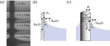
(see figure 1
a). The motion by which the initially flat interface transformed to an equilibrium meniscus was characterized using two dimensionless parameters: the size of the cylinder
 $$\begin{eqnarray}{\it\epsilon}=R/\ell _{c},\end{eqnarray}$$
where
 $\ell _{c}=({\it\gamma}_{lv}/{\it\rho}_{\ell }g)^{1/2}$
is the capillary length, and the Kapitsa number
 $$\begin{eqnarray}\mathit{Ka}=[{\it\gamma}_{lv}/({\it\rho}_{\ell }^{3}{\it\nu}^{4}g)]^{1/4},\end{eqnarray}$$
(with
 $g$
the acceleration due to gravity) which is the characteristic Reynolds number,
 $\mathit{Re}$
, of capillary–gravity waves. CQ performed careful experiments in each of the four asymptotic regimes that result from this two-dimensional parameter space and determined scaling laws for the growth of the meniscus height,
 $h_{m}$
, with time
 $t$
after the cylinder touches the interface.
(a) Images from experiments reported by Clanet & Quéré (Reference Clanet and Quéré2002). Here, a fibre of radius
 $R=0.225~\text{mm}$
touches the interface between air and hexane at
 $t=0$
and a meniscus rises around it. (Images courtesy of Christophe Clanet.) Sketches showing the essential ingredients for determining the scaling of meniscus height
 $h_{m}$
with time
 $t$
are shown for the cases of (b) rise next to a vertical wall and (c) rise outside a circular cylinder. The scaling laws for
 $h_{m}(t)$
are found by balancing the force due to the interfacial tension,
 ${\it\gamma}_{lv}$
, with the rate of change of momentum of the meniscus. For details, see text.

In the limit
 $\mathit{Ka}\gg 1$
(equivalent to high
 $\mathit{Re}$
) and large cylinders,
 ${\it\epsilon}\gg 1$
, the problem of the growth of a meniscus is mathematically equivalent to the retraction of a two-dimensional wedge of fluid with a fixed contact angle. This problem was first studied by Keller & Miksis (Reference Keller and Miksis1983) but is important in the coalescence of drops and, as such, has continued to generate interest (see Thompson & Billingham Reference Thompson and Billingham2012, for a review of the literature). Previous studies of axisymmetric geometries have focused on a fixed wedge angle in the far field (Leppinen & Lister Reference Leppinen and Lister2003; Sierou & Lister Reference Sierou and Lister2004). In this paper, we focus on the case of inviscid motion,
 $\mathit{Ka}\gg 1$
, and small cylinders,
 ${\it\epsilon}\ll 1$
, with a fixed contact angle
 ${\it\theta}$
at the cylinder wall. To the best of our knowledge, this does not have a direct analogue in the literature on coalescence and breakup of drops.
2. Previous results
Before developing our own model of the inertial capillary rise around a small cylinder, we summarize existing results for this problem. We begin with the scaling laws given by CQ for the evolution of the meniscus height
 $h_{m}(t)$
.
2.1. Scalings for the dynamics of inertial rise
Motivated by their experimental observations, CQ assumed that the contact angle of the liquid on the wetted body,
 ${\it\theta}$
in figure 1(b,c), is approximately constant during the motion. Using this assumption, they presented scaling analyses for the inertia-dominated dynamics in two particular geometries: (i) a meniscus next to a planar wall (illustrated schematically in figure 1
b) and (ii) a meniscus outside a vertical cylinder (illustrated schematically in figure 1
c). It is the latter case that is of primary interest here, but we consider the former case first for pedagogical reasons.
Following CQ, we consider the force balance on a two-dimensional meniscus of unit width (into the page): the vertical force driving the capillary rise is that from surface tension,
 ${\it\gamma}_{lv}\cos {\it\theta}$
, while the inertia of the meniscus resists rise. Since the mass of the meniscus is not constant (
 $m\sim {\it\rho}_{\ell }{h_{m}}^{2}$
by the assumption of a constant contact angle), Newton’s second law implies that
 ${\it\gamma}_{lv}\cos {\it\theta}\sim \text{d}(m{\dot{h}}_{m})/\text{d}t$
. In scaling terms this immediately yields
 $$\begin{eqnarray}h_{m}\sim ({\it\gamma}_{lv}/{\it\rho}_{\ell })^{1/3}t^{2/3}.\end{eqnarray}$$
This is the well known capillary–inertia scaling first found by Keller & Miksis (Reference Keller and Miksis1983).
In the case of an axisymmetric meniscus rising outside a circular cylinder, CQ follow an argument along the same lines. Because of the finite radius of the cylinder, however, the force from surface tension is now
 ${\it\gamma}_{lv}R\cos {\it\theta}$
, while the mass of the meniscus is
 $m\sim {\it\rho}_{\ell }h_{m}\times h_{m}(R+h_{m})$
. Assuming that
 $h_{m}\gg R$
and making use of Newton’s second law again, we find
 $$\begin{eqnarray}h_{m}\sim ({\it\gamma}_{lv}R/{\it\rho}_{\ell })^{1/4}t^{1/2}.\end{eqnarray}$$
While the form of the
 $t^{1/2}$
scaling in (2.2) may be familiar from the problem of the surface-tension-driven coalescence of two liquid drops of radius
 $R$
(see Duchemin, Eggers & Josserand Reference Duchemin, Eggers and Josserand2003, for example), there is no clear analogy between the two problems. Indeed, in wedge retraction problems, the
 $t^{2/3}$
scaling of (2.1) is almost generic and so the scaling (2.2) represents a novel twist. However, it is vital to note that a key step in the derivation of (2.2) is the simplifying assumption (made only implicitly by CQ) that
 $h_{m}\gg R$
. If, instead, we had assumed that
 $h_{m}\ll R$
then we would have recovered the classic
 $t^{2/3}$
scaling, (2.1). This difference in scaling is unsurprising since when
 $h_{m}\ll R$
, the curvature of the cylinder is much smaller than the intrinsic curvature of the meniscus and the meniscus cannot ‘feel’ the curvature of the cylinder; it is as if the meniscus were rising against a planar wall. Indeed, one might expect that even in the axisymmetric problem, the scaling
 $h_{m}\sim t^{2/3}$
should be recovered at sufficiently early times since
 $h_{m}\ll R$
must always hold at sufficiently early times. The scaling
 $h_{m}\sim t^{2/3}$
was not, however, reported for small cylinders,
 ${\it\epsilon}\ll 1$
, by CQ.
2.2. The final rise height
For a single cylinder, meniscus rise does not continue indefinitely; rather,
 $h_{m}(t)\rightarrow h_{m}^{\infty }$
, a constant that depends on the contact angle,
 ${\it\theta}$
, and cylinder radius,
 $R$
. Asymptotic results for
 $h_{m}^{\infty }$
have been determined in the limit of very small cylinders,
 ${\it\epsilon}=R/\ell _{c}\ll 1$
, up to second order in
 ${\it\epsilon}$
(James Reference James1974; Lo Reference Lo1983). For our purposes, the leading-order result
 $$\begin{eqnarray}\frac{h_{m}^{\infty }}{\ell _{c}}\approx {\it\epsilon}\cos {\it\theta}\left[\log \left(\frac{4}{{\it\epsilon}(1+\sin {\it\theta})}\right)-{\it\Gamma}_{em}\right]\end{eqnarray}$$
is sufficient. (Here,
 ${\it\Gamma}_{em}=0.5772\dots$
is the Euler–Mascheroni constant.)
A key feature of (2.3) is that
 $h_{m}^{\infty }\sim R\log (\ell _{c}/R)$
. For extremely small cylinder radii,
 ${\it\epsilon}=R/\ell _{c}\lll 1$
, the equilibrium rise height
 $h_{m}^{\infty }\gg R$
and so
 $h_{m}\gg R$
for sufficiently late times. At such late times it is possible that the motion is no longer inertial so that the scaling argument in § 2.1 breaks down. However, it is also possible that inertia continues to play an important role close to the equilibrium height (Quéré (Reference Quéré1997) observed inertial oscillations about equilibrium for the capillary rise within a cylinder). Even in this latter scenario, it is not clear whether, for experimentally attainable values of
 ${\it\epsilon}$
,
 $h_{m}/R$
is ever sufficiently large for the scaling law (2.2) to hold. To answer this question, we now formulate a fluid-mechanical model of the inertia-dominated onset of menisci.
3. A model of dynamic meniscus rise
In the experiments of CQ, a cylinder was lowered until it just touched the liquid–gas interface. This marks the beginning of the experiment,
 $t=0$
. Using a cylindrical polar coordinate system centred on the axis of the cylinder, we therefore expect that the boundary condition on the liquid surface will change depending on whether
 $r<R$
(so that the liquid is bounded by the rigid liquid–solid interface) or
 $r>R$
(so that the liquid is bounded by the deformable liquid–gas interface). This change in type of the boundary conditions frequently leads to singularities (see Howison, Morgan & Ockendon Reference Howison, Morgan and Ockendon1997, for example). To weaken this singularity, we instead assume that the cylinder occupies the entire region
 $r<R$
(i.e. at all heights, not just
 $z>0$
as is the case experimentally).
We use the capillary length
 $\ell _{c}=({\it\gamma}_{lv}/{\it\rho}_{\ell }g)^{1/2}$
to non-dimensionalize lengths. This non-dimensionalization introduces the dimensionless cylinder radius
 ${\it\epsilon}=R/\ell _{c}$
of (1.1). From the capillary length, the capillary time
 $t_{c}=(\ell _{c}/g)^{1/2}$
and velocity
 $v_{c}=(g\ell _{c})^{1/2}$
then emerge as the natural time and velocity scales, respectively. We shall use dimensionless variables based on these scales henceforth. The intrinsic velocity and length scales lead to an intrinsic Reynolds number
 $$\begin{eqnarray}\mathit{Re}=\frac{g^{1/2}\ell _{c}^{3/2}}{{\it\nu}}=\mathit{Ka}.\end{eqnarray}$$
It should be noted that
 $\mathit{Ka}\approx 450$
for an air–water interface and
 $\mathit{Ka}\approx 480$
for an air–hexane interface (using parameter values from CQ). Thus, although we will generally be interested in the fluid flow around small objects (the experiments reported by CQ had
 $R\approx 0.1~\text{mm}$
), our model shall assume that the motion is inviscid. For
 $t<0$
, the liquid is stationary, and hence irrotational. Within the limits of Euler’s equations, the flow then remains irrotational for all times, i.e.
 $\boldsymbol{u}=\boldsymbol{{\rm\nabla}}{\it\varphi}$
. Assuming that the fluid is incompressible, we have that
 $$\begin{eqnarray}{\rm\nabla}^{2}{\it\varphi}=0,\end{eqnarray}$$
in the liquid region:
 $r>{\it\epsilon}$
,
 $-\infty <z<h(r,t)$
, where
 $z=h(r,t)$
is the vertical position of the interface, which is, as yet, undetermined.
The kinematic boundary condition requires that
 $$\begin{eqnarray}\left.\frac{\partial {\it\varphi}}{\partial z}\right|_{z=h(r,t)}=\frac{\text{D}h}{\text{D}t}\end{eqnarray}$$
for
 $r>{\it\epsilon}$
. Similarly, Bernoulli’s theorem using the dynamic boundary condition for the pressure jump across the interface due to capillarity gives
 $$\begin{eqnarray}\frac{\partial {\it\varphi}}{\partial t}+\frac{1}{2}|\boldsymbol{{\rm\nabla}}{\it\varphi}|^{2}-\frac{1}{r}\frac{\partial }{\partial r}\left[\frac{rh_{r}}{(1+h_{r}^{2})^{1/2}}\right]+h=0\end{eqnarray}$$
on
 $z=h(r,t)$
, where
 $h_{r}=\partial h/\partial r$
. In the latter equation we include the contribution from hydrostatic pressure,
 $h$
, so that the meniscus eventually reaches its equilibrium height, which is determined by a balance between the last two terms in this equation.
The capillary rise is driven by the contact angle condition at the cylinder wall. Ordinarily, the dynamic contact angle,
 ${\it\theta}_{d}$
, depends on the velocity of the contact line with a relationship that is determined by a balance between capillarity and viscosity (de Gennes et al.
Reference de Gennes, Brochard-Wyart and Quéré2003; Snoeijer & Andreotti Reference Snoeijer and Andreotti2013). In inertia-dominated motion, however, experiments suggest that
 ${\it\theta}_{d}$
is approximately constant, as observed by CQ but also independently (see Ablett Reference Ablett1923; Vella, Lee & Kim Reference Vella, Lee and Kim2006, for example). Here, therefore, we take
 ${\it\theta}_{d}={\it\theta}$
, the equilibrium contact angle, throughout the motion. We then have that
 $$\begin{eqnarray}\left.\frac{\partial h}{\partial r}\right|_{r={\it\epsilon}}=-\!\cot {\it\theta},\end{eqnarray}$$
while the impenetrability of the cylinder ensures that
 $$\begin{eqnarray}\left.\frac{\partial {\it\varphi}}{\partial r}\right|_{r={\it\epsilon}}=0.\end{eqnarray}$$
Finally, far from the cylinder we expect the fluid velocity and interface displacement to decay, i.e.
 $$\begin{eqnarray}|\boldsymbol{{\rm\nabla}}{\it\varphi}|\rightarrow 0\quad \text{as}~r^{2}+z^{2}\rightarrow \infty ,\quad h(r,t)\rightarrow 0\quad \text{as}~r\rightarrow \infty .\end{eqnarray}$$
A numerical solution of (3.2)–(3.7) is calculated using the finite element method (see Eriksson et al.
Reference Eriksson, Estep, Hansbo and Johnson1996, for example) on the domain
 $-L_{z}<z<h(r,t),{\it\epsilon}<r<L_{r}$
. Here,
 $L_{z}$
and
 $L_{r}$
are sufficiently large that increasing them has negligible effect on the solution. We compute the solution at a discrete set of points in time
 $t=t_{0},t_{1},t_{2},\dots \,$
, and write
 $h^{(n)}(r)=h(r,t_{n}),{\it\phi}^{(n)}(r,z)={\it\phi}(r,z,t_{n})$
. When computing
 $h^{(n)}$
and
 ${\it\phi}^{(n)}$
at time
 $t_{n}$
the time derivatives in (3.3) and (3.4) are approximated implicitly by, for example,
 $(h^{(n)}(r)-h^{(n-1)}(r))/(t_{n}-t_{n-1})$
. The solution for both
 $h^{(n)}$
and
 ${\it\phi}^{(n)}$
at each time step was obtained through a coupled approximation of the partial differential equations satisfied by these variables. A mesh of quadrilateral elements was used, and this mesh was updated at each time step to take account of the evolution in the computational domain as
 $h(r,t)$
varies. The mesh was generated with a higher density of nodes in the region around
 $z=h(r,t),r={\it\epsilon}$
. Both the nodal spacing of the mesh and the time step were reduced until the results (presented later) were visually indistinguishable from those generated using a finer mesh and a shorter time step.
4. Numerical results
To arrive at the model problem given by (3.2)–(3.7) we have made a number of simplifying assumptions. Most notable among these are (i) that the contact angle is constant throughout the motion, (ii) that the meniscus motion as a cylinder touches the interface should be similar to that caused by a cylinder that instantaneously appears in the volume
 $r<{\it\epsilon}$
,
 $-\infty <z<\infty$
and (iii) that the fluid motion is described by a velocity potential. To test whether these assumptions are reasonable in a model of the onset of menisci, we now compare the results of our numerical simulations with experimental results (digitized directly from figure 16 of CQ).
The only unknown parameter in our model is the equilibrium contact angle
 ${\it\theta}$
. To determine
 ${\it\theta}$
, we fitted the static meniscus shape in images of the original experiments (kindly provided by Christophe Clanet) to numerical solutions of the Laplace–Young equation. We found that
 ${\it\theta}=13^{\circ }$
minimizes the residual of this fit and so take
 ${\it\theta}=13^{\circ }$
in all comparisons between theory and experiment reported in this paper.
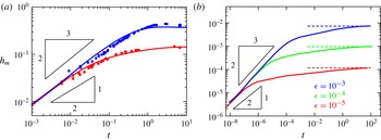
Numerical results for the evolution of the meniscus height,
 $h_{m}=h({\it\epsilon},t)$
, for cylinders of different radius,
 ${\it\epsilon}=R/\ell _{c}$
, all with contact angle
 ${\it\theta}=13^{\circ }$
. (a) Numerical results for
 ${\it\epsilon}=0.15$
(blue curve) and
 ${\it\epsilon}=0.037$
(red curve) compare favourably with the experimental results of CQ with
 ${\it\epsilon}=0.153$
(blue squares) and
 ${\it\epsilon}=0.037$
(red circles) respectively. (b) Numerical results for
 ${\it\epsilon}=10^{-5}$
(red),
 ${\it\epsilon}=10^{-4}$
(green) and
 ${\it\epsilon}=10^{-3}$
(blue) show that the classic scaling law
 $h_{m}\sim t^{2/3}$
is observed at early times but not the CQ scaling
 $h_{m}\sim t^{1/2}$
. Dashed lines show the equilibrium rise height,
 $h_{m}^{\infty }$
, for each value of
 ${\it\epsilon}$
. (Here, lengths are non-dimensionalized by
 $\ell _{c}$
and times by
 $t_{c}=(\ell _{c}/g)^{1/2}$
.)

Figure 2(a) shows a comparison between the numerical solution of our model and the experimental results of CQ for the evolution of the meniscus height
 $h_{m}(t)=h({\it\epsilon},t)$
. (Here, data for the two extremal cylinder radii presented by CQ, subject to
 ${\it\epsilon}\ll 1$
, are used.) We see that the agreement between the model results and experiments is good, despite the simplicity of the model, in particular the assumptions (i)–(iii) listed above, and the lack of any fitting parameter. We conclude from this agreement that the model does indeed capture the essential physics exhibited by the experimental system.
However, we note that the numerical solutions do not show any compelling evidence for the
 $t^{1/2}$
scaling expected on the basis of (2.2). Instead, it seems that at early times,
 $t\ll 1$
, the meniscus height
 $h_{m}\propto t^{2/3}$
; at later times the meniscus growth gradually slows to reach the final equilibrium meniscus height,
 $h_{m}^{\infty }$
. While this accords with our expectations for the moderate cylinder radii used experimentally, the discussion of § 2 suggested that the
 $t^{1/2}$
scaling might be observed if
 ${\it\epsilon}\ll h_{m}$
during the inertial evolution, i.e. if
 ${\it\epsilon}\lll 1$
. Figure 2(b) therefore shows numerical results for
 $10^{-5}\leqslant {\it\epsilon}\leqslant 10^{-3}$
. Again, we see no sign of the
 $t^{1/2}$
scaling.
It could be argued that our numerical simulations do not reach sufficiently small values of
 ${\it\epsilon}$
. (Even with
 ${\it\epsilon}=10^{-5}$
,
 $h_{m}^{\infty }/{\it\epsilon}\lesssim 10$
.) To try to provide more conclusive evidence that this is not the case, we now move on to extract some universal dynamics for this problem. In particular, we show that it is possible to collapse data for the evolution of the meniscus height with different cylinder radii onto a single master curve (provided that
 ${\it\theta}$
is constant and
 $t\ll 1$
so that gravity is unimportant). This gives us another tool with which to probe the possible scaling laws.
5. A family of similarity solutions
It is well known that the two-dimensional version of the problem described in § 3 with negligible gravity admits a similarity solution with spatial scale
 $t^{2/3}$
(Keller & Miksis Reference Keller and Miksis1983; Billingham & King Reference Billingham and King1995). Even when gravity is present (via the hydrostatic pressure term in (3.4)), its influence may be neglected at sufficiently early times,
 $t\ll 1$
; the classic similarity solution of Keller & Miksis (Reference Keller and Miksis1983) re-emerges to govern the early time dynamics (see Vella & Metcalfe Reference Vella and Metcalfe2007; Duchemin & Vandenberghe Reference Duchemin and Vandenberghe2014, for example). Given this generic behaviour, it is clear that when the length scale associated with the similarity solution is small compared with the radius of the cylinder, i.e.
 $t^{2/3}\ll {\it\epsilon}$
, then the curvature of the cylinder cannot enter the problem and we must recover the classic two-dimensional problem (Keller & Miksis Reference Keller and Miksis1983). From this idea, it follows naturally that even at later times (but retaining
 $t\ll 1$
) it must be the effective size of the cylinder relative to the length scale of the similarity solution that determines the dynamics. Of course, as the evolution progresses this effective cylinder size evolves too; nevertheless we introduce the rescaled cylinder radius
 $$\begin{eqnarray}\mathscr{R}={\it\epsilon}/t^{2/3}\end{eqnarray}$$
and seek a similarity-type solution by letting
 $$\begin{eqnarray}{\it\rho}=(r-{\it\epsilon})/t^{2/3},\quad {\it\zeta}=z/t^{2/3},\quad {\it\eta}({\it\rho};\mathscr{R})=h(r,t)/t^{2/3},\quad {\it\Phi}({\it\rho},{\it\zeta};\mathscr{R})={\it\varphi}(r,t)/t^{1/3}.\end{eqnarray}$$
We find that Laplace’s equation (3.2) becomes
 $$\begin{eqnarray}\frac{\partial ^{2}{\it\Phi}}{\partial {\it\zeta}^{2}}+\frac{\partial ^{2}{\it\Phi}}{\partial {\it\rho}^{2}}+\frac{1}{\mathscr{R}+{\it\rho}}\frac{\partial {\it\Phi}}{\partial {\it\rho}}=0\end{eqnarray}$$
in
 $0\leqslant {\it\rho}<\infty$
,
 $-\infty <{\it\zeta}\leqslant {\it\eta}({\it\rho};\mathscr{R})$
, while the kinematic boundary condition (3.3) and Bernoulli equation (3.4) become
 $$\begin{eqnarray}\frac{\partial {\it\Phi}}{\partial {\it\zeta}}=\frac{2}{3}\left({\it\eta}-{\it\rho}\frac{\partial {\it\eta}}{\partial {\it\rho}}-\mathscr{R}\frac{\partial {\it\eta}}{\partial \mathscr{R}}\right)+\frac{\partial {\it\Phi}}{\partial {\it\rho}}\frac{\partial {\it\eta}}{\partial {\it\rho}}\end{eqnarray}$$
and
 $$\begin{eqnarray}\displaystyle & & \displaystyle \frac{1}{3}{\it\Phi}-\frac{2}{3}\left({\it\zeta}\frac{\partial {\it\Phi}}{\partial {\it\zeta}}+{\it\rho}\frac{\partial {\it\Phi}}{\partial {\it\rho}}+\mathscr{R}\frac{\partial {\it\Phi}}{\partial \mathscr{R}}\right)+\frac{1}{2}\left[\left(\frac{\partial {\it\Phi}}{\partial {\it\rho}}\right)^{2}+\left(\frac{\partial {\it\Phi}}{\partial {\it\zeta}}\right)^{2}\right]\nonumber\\ \displaystyle & & \displaystyle \quad =\frac{1}{\mathscr{R}+{\it\rho}}\frac{{\it\eta}_{{\it\rho}}}{(1+{\it\eta}_{{\it\rho}}^{2})^{1/2}}+\frac{{\it\eta}_{{\it\rho}{\it\rho}}}{(1+{\it\eta}_{{\it\rho}}^{2})^{3/2}}-t^{4/3}{\it\eta}\end{eqnarray}$$
respectively, with each evaluated on
 ${\it\zeta}={\it\eta}({\it\rho};\mathscr{R})$
. It should be noted that in these latter two equations, derivatives with respect to the rescaled cylinder radius
 $\mathscr{R}$
arise from use of the chain rule for time derivatives; this reflects the change of the effective cylinder size during the motion (Vella & Li Reference Vella and Li2010).
Laplace’s equation (5.3) is to be solved together with the boundary conditions (5.4), (5.5) as well as (3.5)–(3.7), which take the similarity form
 $$\begin{eqnarray}\left.\frac{\partial {\it\eta}}{\partial {\it\rho}}\right|_{{\it\rho}=0}=-\!\cot {\it\theta};\quad \left.\frac{\partial {\it\Phi}}{\partial {\it\rho}}\right|_{{\it\rho}=0}=0;\quad |\boldsymbol{{\rm\nabla}}{\it\Phi}|\rightarrow 0\quad \text{as}~{\it\rho}^{2}+{\it\zeta}^{2}\rightarrow \infty ;\quad {\it\eta}\rightarrow 0\quad \text{as}~{\it\rho}\rightarrow \infty .\end{eqnarray}$$
For early times
 $t\ll 1$
, all explicit mention of time is lost from the system (5.3)–(5.6). However, the rescaled cylinder radius
 $\mathscr{R}$
remains as a parameter: for a constant cylinder radius
 ${\it\epsilon}$
, the changing value of
 $\mathscr{R}$
as time evolves ensures that time remains in the problem, albeit implicitly. While it may seem that we have therefore not gained anything by the transformation (5.2), we shall see that we do, in fact, gain new insight into the dynamics.
We first consider the limit
 $t\ll {\it\epsilon}^{3/2}\ll 1$
. In this case we have that
 $\mathscr{R}={\it\epsilon}/t^{2/3}\gg 1$
, so that the terms involving
 $1/(\mathscr{R}+{\it\rho})$
in (5.3) and (5.5) may be neglected while the
 $t^{4/3}{\it\eta}$
term in (5.5) (corresponding to the effect of gravity) may also be neglected. Making the additional assumption that
 ${\it\Phi}$
and
 ${\it\eta}$
decay sufficiently quickly that the additional terms
 $\mathscr{R}\partial {\it\eta}/\partial \mathscr{R}$
and
 $\mathscr{R}\partial {\it\Phi}/\partial \mathscr{R}$
in (5.4) and (5.5) may be neglected as
 $\mathscr{R}\rightarrow \infty$
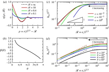
, we find that the system (5.3)–(5.6) reduces to the two-dimensional problem considered by Keller & Miksis (Reference Keller and Miksis1983). This intuition is confirmed in figure 3(a), where we see that the interface shape for large
 $\mathscr{R}$
is close to that found by Keller & Miksis (Reference Keller and Miksis1983). Hence, for
 $t\ll {\it\epsilon}^{3/2}$
we have
 $$\begin{eqnarray}h_{m}={\it\beta}({\it\theta})t^{2/3},\end{eqnarray}$$
where the prefactor
 ${\it\beta}({\it\theta})$
may be determined using the numerical method described by Keller & Miksis (Reference Keller and Miksis1983). (The behaviour of
 ${\it\beta}({\it\theta})$
is plotted in figure 3
b, for completeness.)
The utility of the family of similarity solutions for understanding numerical results. (a) The interface profile plotted in similarity form for the Keller & Miksis (Reference Keller and Miksis1983) problem with
 ${\it\theta}=80^{\circ }$
(black dashed curve) and the solution of the linearized similarity system (5.3)–(5.6) with different values of
 $\mathscr{R}={\it\epsilon}/t^{2/3}$
. For the linearized problem, the displacement may be rescaled arbitrarily; here (3.5) is replaced by
 ${\it\eta}_{{\it\rho}}(0;\mathscr{R})=-1$
. (b) The dependence of
 ${\it\beta}$
on the contact angle
 ${\it\theta}$
for a plane,
 $\mathscr{R}=\infty$
(following Keller & Miksis Reference Keller and Miksis1983, for example). (c) Full numerical results for a range of cylinder radii collapse at early times (
 $t\ll 1$
corresponds to
 $\mathscr{R}\gg {\it\epsilon}$
) onto the numerically determined solutions of the similarity system (5.3)–(5.6) (black dashed curve). Here,
 ${\it\theta}=85^{\circ }$
. In these rescaled variables, the CQ scaling (2.2) would require that
 ${\it\eta}(0;\mathscr{R})\sim \mathscr{R}^{1/4}$
, see (5.8). (d) Numerical results with
 ${\it\epsilon}=10^{-3}$
and different contact angles
 ${\it\theta}$
show qualitatively similar behaviour but that the dependence on
 ${\it\theta}$
cannot simply be rescaled. Dashed lines show the predicted behaviour when equilibrium is reached,
 $t\gg 1$
, corresponding to
 $h_{m}=h_{m}^{\infty }$
. Dash-dotted lines show the value of
 ${\it\beta}({\it\theta})=h_{m}/t^{2/3}$
in the corresponding two-dimensional problem, which is recovered in the limit
 $t\ll 1$
,
 $\mathscr{R}\gg 1$
.

With finite
 $\mathscr{R}$
but
 $t\ll 1$
, the motion is described by a family of similarity-like solutions parametrized by the rescaled cylinder radius
 $\mathscr{R}$
and the contact angle
 ${\it\theta}$
. As a result, we expect that data with fixed
 ${\it\theta}$
and different cylinder radii should collapse when
 $h_{m}/t^{2/3}$
is plotted as a function of
 $\mathscr{R}={\it\epsilon}/t^{2/3}$
. Figure 3(c) shows that such a collapse is observed in the numerical simulations with various radii and constant
 ${\it\theta}$
; this collapse breaks down, however, once
 $t\gtrsim 1$
,
 $\mathscr{R}\lesssim {\it\epsilon}$
, at which point the role of the hydrostatic pressure term in (5.5) can no longer be neglected. As the contact angle is varied, similar curves are obtained (figure 3
d).
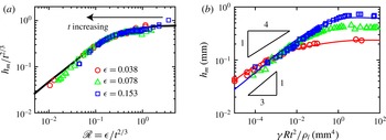
On plotting the experimental data from CQ in the way suggested by the family of similarity solutions, we observe an excellent collapse onto a single master curve (see figure 4
a). On comparing this collapse with that suggested by the CQ scaling (2.2) (plotted in figure 4
b), we see that the parameter
 $\mathscr{R}={\it\epsilon}/t^{2/3}$
arguably provides a better account of the effect of the cylinder radius. Furthermore, we see that even where figure 4(b) suggests that the experimental data leave the CQ scaling (2.2) to tend to the equilibrium rise height,
 $h_{m}^{\infty }$
, the rescaled height
 $h_{m}(t)/t^{2/3}$
remains on a master curve when plotted as a function of
 $\mathscr{R}$
. We therefore conclude that the family of similarity solutions describes a universal dynamics that takes place after the initial
 $t^{2/3}$
behaviour but before the meniscus approaches equilibrium. (We emphasize that precisely the same data set is plotted in figure 4
a,b.)
The utility of the family of similarity solutions for understanding experimental results (captured from figure 16 of CQ). (a) Experimental results (points) and the results of the full numerical simulations with
 ${\it\epsilon}=10^{-5}$
,
 ${\it\theta}=13^{\circ }$
(solid curve) may be collapsed onto a master curve by using the similarity rescaling (5.1). (b) A plot of the same data points as in (a) but in the rescaling suggested by (2.2) shows good initial collapse that breaks down later on.

The collapse observed in figure 4(a) demonstrates that the cylinder radius
 $R$
does affect the evolution of the meniscus height and, further, that its effect as the rescaled radius
 $\mathscr{R}={\it\epsilon}/t^{2/3}$
evolves is captured by the family of similarity solutions with the appropriate value of
 ${\it\theta}$
. However, the observed collapse of the experimental data can only be consistent with the CQ scaling law (2.2) if
 $$\begin{eqnarray}{\it\eta}(0;\mathscr{R})\sim \mathscr{R}^{1/4}\end{eqnarray}$$
for some values of
 $\mathscr{R}$
. To search for such a behaviour, we solve the linearized version of the problem (5.3)–(5.6) using a finite difference scheme. (It should be noted that to enable us to start with
 $\mathscr{R}=\infty$
we use the substitution
 $\mathscr{S}=1/\mathscr{R}$
starting with
 $\mathscr{S}=0$
and solving the resulting problem using first-order finite differences on a rectangular grid in the spatial variables
 ${\it\rho}$
and
 ${\it\zeta}$
. We then step forward to consider
 $\mathscr{S}>0$
, using second-order differences in
 $\mathscr{S}$
.) The solution of this linearized problem can be rescaled to give the results for any contact angle close to
 ${\it\theta}={\rm\pi}/2$
. The results of this calculation agree well with the results of our full numerical simulations for
 ${\it\theta}=85^{\circ }$
(see figure 3
c). Again, we do not see any indication that a scaling of the form (5.8) is present.
6. Conclusions
We have presented a fluid-mechanical model for the inertial growth of a meniscus external to a circular cylinder. Our potential flow model with a constant contact angle is able to quantitatively reproduce previously published experimental data (CQ) for a range of cylinder radii. We have assumed that inertia dominates viscosity and, further, that the dynamic contact angle is equal to the static contact angle throughout the motion. In reality these assumptions must break down at the very earliest times: according to the similarity solution the viscous dissipation
 $u_{xx}/\mathit{Re}\sim t^{-5/3}/\mathit{Re}$
will, in fact, dominate the inertial terms
 $u_{t},uu_{x}\sim t^{-4/3}$
for
 $t\lesssim \mathit{Re}^{-3}\sim 10^{-8}$
(corresponding to
 $t\lesssim 10^{-10}~\text{s}$
in dimensional terms). Similarly, the undeformed interface must first react to the touch down of the cylinder. After these earliest transients, but with
 $t\lesssim {\it\epsilon}^{3/2}$
, the meniscus height grows like
 $t^{2/3}$
– the radius of the cylinder does not play a role and the problem reduces to the two-dimensional one studied by Keller & Miksis (Reference Keller and Miksis1983). At later times the evolution of the meniscus height with time is governed by a family of similarity solutions parametrized by the rescaled cylinder radius
 $\mathscr{R}={\it\epsilon}/t^{2/3}=R\left[{\it\rho}_{\ell }/({\it\gamma}_{lv}t^{2})\right]^{1/3}$
, provided that
 $t\ll 1$
(so that gravity may be neglected). The introduction of the parameter
 $\mathscr{R}$
allows us to collapse previous experimental data for the meniscus height with different cylinder radii onto a master curve.
Our analysis suggests that the scaling law (2.2) proposed by CQ rests on an implicit assumption (that
 $h_{m}\gg R$
) that is not consistent with the behaviour of menisci growing in the presence of gravity. (We emphasize that this inconsistency occurs only in the regime
 ${\it\epsilon}\ll 1$
,
 $\mathit{Ka}\gg 1$
and does not affect the results reported by CQ in the three other regimes considered there.) It seems likely that the misidentification of the scaling law (2.2) in experiments was the result of the data ‘turning away’ from the
 $t^{2/3}$
behaviour and towards equilibrium. Nevertheless, it remains possible that this scaling is achieved in the limit of extremely small cylinders or, equivalently, extremely weak gravity. We hope that our model of the problem and introduction of the parameter
 $\mathscr{R}$
may help to both inspire and interpret future experimental work on this rich fundamental problem.
Acknowledgements
This publication is based on work supported in part by Award No KUKC1-013-04, made by King Abdullah University of Science and Technology (KAUST). We are grateful to the participants of the Oxford–Princeton Collaborative Workshop Initiative 2014 for their comments on this work and to C. Clanet for sharing the original experimental images in figure 1.