





1 Introduction
The recent breakthroughs at the National Ignition Facility (NIF)[
Reference Kritcher, Zylstra, Weber, Hurricane, Callahan, Clark, Divol, Hinkel, Humbird, Jones, Lindl, Maclaren, Strozzi, Young, Allen, Bachmann, Baker, Braun, Brunton, Casey, Chapman, Choate, Dewald, Di Nicola and Edwards
1
] have galvanized the attention of the scientific community, and society in general, on the topic of inertial confinement fusion (ICF) for the future production of energy. In this context, it has become essential to look for complementary/alternative approaches that could be more compatible than indirect drive with the needs for inertial fusion energy (IFE). This drives the attention on direct-drive ICF and, in particular, on the shock ignition approach[
Reference Betti, Zhou, Anderson, Perkins, Theobald and Solodov
2
], which can relax the requirements on irradiation uniformity and reduce the impact of Rayleigh–Taylor hydrodynamics instability, which can be generated by the nonuniformity of direct-drive irradiation. One critical question in shock ignition is that the final ‘ignition’ laser spike, at intensities up to
${10}^{16}$
 W/cm2, is expected to trigger the onset of strong parametric instabilities and the production of hot electrons. Several recent works have highlighted the impact of parametric instabilities: stimulated Raman scattering (SRS), stimulated Brillouin scattering (SBS) and two-plasmon decay (TPD)[
Reference Lindl, Landen, Edwards, Moses and Team
3
–
Reference Nakatsuji, Kawasaki, Idesaka, Matsuura, Tanaka, Sato, Nagatomo, Sentoku, Takagi, Cristoforetti, Batani, Ph. Nicolaï, Yogo, Fujioka and Shigemori
6
]. As for hot electrons, it has already been pointed out that, unlike in conventional ICF, in the context of shock ignition, they could play a positive role in increasing the final pressure.[
Reference Kawasaki, Hironaka, Maeda, Iwasaki, Tanaka, Miyanishi, Nagatomo, Fujioka, Ozaki, Kodama, Matsuoka, Batani, Trela, Nicolaï and Shigemori
7
,
Reference Shang, Betti, Hu, Woo, Hao, Ren, Christopherson, Bose and Theobald
8
] This requires a careful characterization of the hot electron source, which has been the goal of several papers[
Reference Filippov, Khan, Tentori, Gajdos, Martynenko, Dudzak, Koester, Zeraouli, Mancelli, Baffigi, Gizzi, Pikuz, Nicolaï, Woolsey, Fedosejevs, Krus, Juha, Batani, Renner and Cristoforetti
9
–
Reference Trela, Theobald, Anderson, Batani, Betti, Casner, Delettrez, Frenje, Glebov, Ribeyre, Solodov, Stoeckl and Stoeckl
12
], including our previous paper[
Reference Tentori, Colaitis, Theobald, Casner, Raffestin, Ruocco, Trela, Le Bel, Anderson, Wei, Henderson, Peebles, Scott, Baton, Pikuz, Betti, Khan, Woolsey, Zhang and Batani
13
]. This paper was indeed focused firstly on the precise characterization of the hot electron sources through the simultaneous use of multiple diagnostics, and secondly on the effects of hot electrons on shock generation and target hydrodynamics. In particular, the target included a Cu tracer layer, which produced characteristic K
${}_{\alpha }$
 radiation when impacted by the flux of laser-generated hot electrons. The present paper reports the results of a follow-up experiment also performed at the OMEGA EP laser facility in which we added an external magnetic field to the experimental setup in order to study the effects of magnetic fields on laser–target interaction, on hot electron generation and propagation in the target and finally on shock dynamics. In particular, our initial naïve expectation was that the addition of an external magnetic field would have deviated the hot electron trajectories, preventing them from reaching the Cu fluor layer, thus producing a reduction in K
${}_{\alpha }$
 signal. This was also confirmed by simple Monte Carlo simulations with an external magnetic field in which hot electrons propagated in a cold target (no plasma effects). The results of the experiment have proven to be quite different, a puzzling result that has shone light on some interesting physics related to hot electron propagation in laser-irradiated targets with plasma formation.
2 Experimental setup
The experimental setup (Figure 1) is essentially the same as that in our previous paper[
Reference Tentori, Colaitis, Theobald, Casner, Raffestin, Ruocco, Trela, Le Bel, Anderson, Wei, Henderson, Peebles, Scott, Baton, Pikuz, Betti, Khan, Woolsey, Zhang and Batani
13
]. In planar geometry, we drive a shock in a plastic target (CH) with one or two OMEGA EP beams (no phase plate, no smoothing by spectral dispersion (SSD)) using a 1 ns square pulse (from
$I=5\times {10}^{15}$
 to
${10}^{16}$
 $\mathrm{W}/{\mathrm{cm}}^2$
 ), an intensity at which a non-neglectable number of hot electrons are generated. These were characterized by the simultaneous measurement of bremsstrahlung emission and K
${}_{\alpha }$
 emission (8.05 keV) from the buried copper layer inside the target. Parametric instabilities were monitored through a sub-aperture backscatter streak (SABS) diagnostic. Shock dynamics was diagnosed through side X-ray radiography using a vanadium backlighter. However, while in Ref. [Reference Tentori, Colaitis, Theobald, Casner, Raffestin, Ruocco, Trela, Le Bel, Anderson, Wei, Henderson, Peebles, Scott, Baton, Pikuz, Betti, Khan, Woolsey, Zhang and Batani13] we used a framing camera (providing 16 bi-dimensional images at different times), here we used a streak camera (providing a single (x,t) image for each laser shot). Also, we added a streak optical pyrometry (SOP) diagnostic for shock chronometry looking at the rear side of the stepped target. Finally, of course, the main change was the introduction of an external quasi-static magnetic field reaching 30 T at the target using a magneto-inertial fusion electrical discharge system (MIFEDS) pulsed device[
Reference Fiksel, Agliata, Barnak, Brent, Chang, Folnsbee, Gates, Hasset, Lonobile, Magoon, Mastrosimone, Shoup and Betti
14
]. The field was applied transversally with respect to the hot electron/laser propagation direction to affect hot electron trajectories. Figure 2 shows the positioning of the MIFEDS device with respect to the target and laser beam, and Figure 3 shows a map of the produced magnetic field.
Schematic of the experimental setup.

Figure 1 Long description
The diagram is organized from left to right. On the far left, a three-dimensional coordinate system defines Z as vertical, Y as horizontal, and X as depth. A large red arrow labeled Laser ~7 times 10 super 15 W/cm super 2 points right toward a multi-layered target. The target consists of a C H 175 μm layer, a C u 25 μm layer, and a C H 300 μm layer with a 20 μm step. Green arrows labeled Hot electrons originate from the laser impact point and pass through the target layers.
Diagnostic outputs are connected to the target by thin black arrows.
- At the top, a horizontal heat map labeled Spectrum K sub alpha shows a bright intensity peak.
- In the center right, a dark blue square is labeled K sub alpha image.
- At the bottom right, a plot labeled Shock breakout shows a time-calibrated S O P image with position on the Y-axis and time on the X-axis, featuring a vertical black line and a diverging signal pattern.
Positioning of the MIFEDS device with respect to the target and the laser beams. The target is positioned at 0.8 mm from the mid plane of the MIFEDS device.

Figure 2 Long description
The diagram illustrates a complex laser-plasma experimental geometry.
* Diagnostic Axis: Starting from the bottom-left, a yellow line passes through three vertical plates: a pink Streak camera slit, a green Imaging slit, and a blue Line-of-sight shield.
* Interaction Point: The yellow line terminates at the Main target, a small blue and gold cylinder.
* Laser Beams: To the right of the target, two sets of beams converge. Two purple backlighter beams (B 2, B 3) and two red shock beams (B 1, B 4) are shown as conical projections.
* Shielding: Behind the target are a grey C H shield and an orange V foil.
* Magnetic Field: Below the target is a large magenta and gold M I F E D S coil. A black arrow labeled B field points upward from the coil toward the target.
* Coordinate System: A three-axis coordinate system (x, y, z) is positioned to the left of the M I F E D S coil to define the spatial orientation.
Map of the magnetic field produced by the MIFEDS showing (black circle) the position of the target. The white spots in the figure represent the coil turns in the x–z plane at y = 0 m. The position of the target is z = 0 m and its diameter is 0.5 mm, as shown in the figure. The main magnetic field points in the ‘Z’ direction, aligned with the coil’s axis. The cylinder’s axis is perpendicular to this direction. The magnetic field lines pass across the cylinder, perpendicular to the laser axis. The field strength varies across both the target and the laser spot, decreasing from one side to the other. Consequently, one side of the laser interacts with a region closer to 20 T, while the opposite side encounters a field nearer to 50 T.

Figure 3 Long description
A 2D spatial plot in the x-z plane at y = 0.00 m. The horizontal axis represents distance in meters from -0.003 to 0.003, and the vertical axis represents distance in meters from -0.003 to 0.003.
* At the center, a black circle indicates the target position at z = 0.00 m with a diameter of 0.5 mm.
* White spots arranged in vertical columns on either side of the center represent the coil turns.
* A horizontal arrow labeled Z points to the right, indicating the direction of the main magnetic field.
* The magnetic field strength B sub z in Tesla is shown via a color scale on the right, ranging from blue (5 T) to red (65 T).
* The highest field intensity (red, 60 to 65 T) is concentrated near the inner coil turns.
* The field strength decreases as it moves away from the coils. The target circle sits in a gradient region where the field strength varies from approximately 50 T on its left side to 20 T on its right side.
* The outermost regions at the top and bottom edges are shaded blue, indicating the lowest field strength below 5 T.
The experiment was performed in the target chamber of the four-beam OMEGA EP laser facility[
Reference Waxer, Guardalben, Kelly, Kruschwitz, Qiao, Begishev, Bromage, Dorrer, Edwards, Folnsbee, Jacobs, Jungquist, Kessler, Kidder, Loucks, Marciante, Maywar, Mccrory, Meyerhofer and Rigatti
15
] at the Laboratory for Laser Energetics. One or two high-intensity ultraviolet (UV) interaction beams (B1, B4) (
$\lambda =351$
 nm, beam energy of
$\sim$
 1.25 kJ,
$f/6.5$
 ) irradiated a multi-layer target to produce a strong shock wave and generate hot electrons. The beams were tightly focused on the target surface without phase plates to a focal spot size of approximately
$130\;\mu \mathrm{m}$
 . Planar targets consisted of two layers (175 or 250 μm CH/20 or 10 μm Cu) fabricated to 500 μm diameter disks. A few shots were instead realized using targets with 4 mm diameter disks. The rear side of some targets was a thick CH slab (300 μm) aiming at inhibiting hot electron recirculation. A 20 μm step was machined on the rear side to obtain a velocity measurement from shock breakout. The interaction lasers impinged on the front of the 175 μm (or 250 μm) thick CH layer at an angle of incidence of 23° with respect to the target normal. The total yield of Cu
$\mathrm{K}_{\alpha }$
 was measured by a calibrated zinc von Hamos (ZnVH) X-ray spectrometer[
Reference Boutoux, Batani, Burgy, Ducret, Forestier-Colleoni, Hulin, Rabhi, Duval, Lecherbourg, Reverdin, Batani, Szabo, Bastiani-Ceccotti, Consoli, Curcio, De angelis, Ingenito, Baggio and Raffestin
16
]. This spectrometer uses a curved highly oriented pyrolytic graphite (HOPG) crystal in von Hamos geometry to diagnose the X-ray spectrum in the range of 7–10 keV. A high-resolution X-ray spectrometer (HRS) was used with a spherically bent Si [220] crystal coupled to a charge-coupled device to measure the time-integrated X-ray emission in the 7.97–8.11 keV range[
Reference Boutoux, Batani, Burgy, Ducret, Forestier-Colleoni, Hulin, Rabhi, Duval, Lecherbourg, Reverdin, Batani, Szabo, Bastiani-Ceccotti, Consoli, Curcio, De angelis, Ingenito, Baggio and Raffestin
16
]. The hot-electron-produced bremsstrahlung radiation was diagnosed by two time-integrating hard X-ray spectrometers (bremsstrahlung MeV X-ray spectrometers (BMXSs))[
Reference Boutoux, Batani, Burgy, Ducret, Forestier-Colleoni, Hulin, Rabhi, Duval, Lecherbourg, Reverdin, Batani, Szabo, Bastiani-Ceccotti, Consoli, Curcio, De angelis, Ingenito, Baggio and Raffestin
16
] at
$25{}^{\circ}$
 and
$65{}^{\circ}$
 off the target rear normal, respectively. The instruments are composed of a stack of 15 imaging plates (IPs) of MS type[
Reference Boutoux, Batani, Burgy, Ducret, Forestier-Colleoni, Hulin, Rabhi, Duval, Lecherbourg, Reverdin, Batani, Szabo, Bastiani-Ceccotti, Consoli, Curcio, De angelis, Ingenito, Baggio and Raffestin
16
], alternated by filters of different metals.
3 Experimental results
Table 1 shows a summary of the shots performed in the experiment.
Summary of experimental shots with applied magnetic fields and without the magnetic field.

Table 1 Long description
The table consists of six columns: Shot No., Target C H / C u forward slash C H in micrometers, Target diameter in millimeters, Beams driver, Beam backlighter, and B-field.
* Shot 27772: Target 175/20/300, diameter 4, Beams driver B 1, B-field No.
* Shot 27774: Target 175/20/300, diameter 4, Beams driver B 1 plus B 4, B-field No.
* Shot 27776: Target 175/20/300, diameter 4, Beams driver B 1 plus B 4, B-field No.
* Shot 27777: Target 175/20/300, diameter 4, Beams driver B 1, B-field No.
* Shot 28406: Target 175/20/50, diameter 0.5, Beams driver B 4, Beam backlighter B 2, B-field No.
* Shot 28407: Target 175/20/50, diameter 0.5, Beams driver B 1, Beam backlighter B 3, B-field No.
* Shot 28408: Target 175/20/50, diameter 0.5, Beams driver B 1, Beam backlighter B 3, B-field Yes.
* Shot 28410: Target 175/20/50, diameter 0.5, Beams driver B 1 plus B 4, Beam backlighter B 3, B-field No.
* Shot 28412: Target 175/10/50, diameter 0.5, Beams driver B 1, Beam backlighter B 3, B-field No.
* Shot 28413: Target 175/10/50, diameter 0.5, Beams driver B 1, Beam backlighter B 3, B-field Yes.
* Shot 28414: Target 250/10/50, diameter 0.5, Beams driver B 1 plus B 4, Beam backlighter B 3, B-field Yes.
* Shot 28415: Target 250/10/50, diameter 0.5, Beams driver B 1 plus B 4, Beam backlighter B 3, B-field No.
3.1 Diagnostics of shock dynamics
Shock dynamics was investigated using time-resolved X-ray radiography and active shock breakout (ASBO) diagnostics, which included SOP diagnostics. The SOP diagnostic showed the breakout at the target rear surface, which had a machined step interface. Notice that, in order to completely screen the light coming from the lasers, the four shots in which we used ASBO diagnostics utilized larger targets (4 mm in diameter) as compared to the 0.5 mm diameter of the smaller targets used in other shots. Notice that the size of the Cu layer appears to exceed its real value (20 μm). This discrepancy could be due to different reasons, including image spatial resolution, a possibly slight tilt of the target with respect to the viewing direction or finally the heating of the copper layer producing an expansion, as reported by Tentori et al.[
Reference Tentori, Colaitis, Theobald, Casner, Raffestin, Ruocco, Trela, Le Bel, Anderson, Wei, Henderson, Peebles, Scott, Baton, Pikuz, Betti, Khan, Woolsey, Zhang and Batani
13
]. Figure 4 shows one-dimensional (1D) radiographies recorded on the X-ray streak camera (PJX) showing the trajectory of the shock for two shots with and without the magnetic field. From Figure 4 we can deduce a shock velocity of the order of
$D\approx$
 (250 μm)/(3 ns) = 83 μm/ns. After crossing the Cu layer and the final 300 μm plastic, the shock velocity has considerably slowed down. Indeed, the shock transit time in the rear step is
$\Delta t\approx$
 2.2 ns, giving a shock velocity of
$D\approx 9\;\mu \mathrm{m}/\mathrm{ns}$
 . Figure 5 shows the SOP image from shot 27776. The image displays the laser energy incident on the target. The streak camera does not record any initial light emission because the target is cold; however, as the shocks travel through the material, the resulting heating produces the light captured by the sensor. At
$t=0$
 , some noise is visible due to the onset of the laser pulse. The meaningful instants are
${t}_1$
 and
${t}_2$
 , as highlighted in the figure. Specifically,
${t}_1$
 represents the moment when the shock reaches the rear surface of the target, while
${t}_2$
 represents the shock breakthrough at the step on the rear surface of the target. The value
$\Delta t$
 is defined as the difference between
${t}_1$
 and
${t}_2$
 .
(Top) PJX of shot 28415, two beams, 250 μm CH, without the B-field. (Bottom) PJX of shot 28414, two beams, 250 μm CH, with the B-field. The right-hand column shows the same images, where red and yellow lines represent the likely trajectories of the shock front and the ablation front (guides for the eyes only).

Figure 4 Long description
A four-panel grid of P J X images showing plasma evolution over a 3 n s time scale.
Top-Left Panel: Shot 28415 without a B-field. It shows two horizontal glowing bands of plasma separated by a dark central gap.
Top-Right Panel: The same image as the top-left but with annotations. A white arrow points to a thin horizontal orange bar labeled 10 mu m C u. Below this bar, a red dashed line slopes upward from left to right, and a yellow dashed line follows a shallower upward curve. Black double-headed arrows on the right indicate vertical spatial scales.
Bottom-Left Panel: Shot 28414 with a B-field. The plasma bands appear more structured and elongated compared to the top row. A horizontal arrow at the bottom indicates a 3 n s time duration.
Bottom-Right Panel: The same image as the bottom-left with annotations. It includes the horizontal orange bar and the red and yellow dashed lines representing the shock front and ablation front trajectories. A large blue arrow at the bottom points upward, labeled laser, indicating the direction of energy input. The label 250 mu m C H is positioned near the bottom right.
SOP image for shot 27776. Laser energy on target 2507 J. Target: 175 μm CH + 16 μm Cu + 300(+20) μm CH.

Figure 5 Long description
The left side shows a schematic where a pink laser beam cone is incident on a gray multi-layered target. A dashed horizontal line aligns the target interface with the data plot on the right.
The right side is a streak camera image with Time in n s on the horizontal axis (0 to 40) and Position in pixels on the vertical axis (1100 to 2000). A color scale on the far right indicates intensity from 0 to 2000.
Key features in the streak data include:
* A series of calibration dots along the top edge.
* A faint vertical band near 12 n s.
* Two vertical dashed lines labeled t sub 1 and t sub 2 located at approximately 16 n s and 18.5 n s respectively.
* A prominent, dark vertical emission line at approximately 22 n s.
* A V-shaped expansion pattern originating from the target interface line, widening as time increases from 20 to 40 n s.
* A faint vertical band at 27 n s.
3.2 Diagnostics for parametric instabilities
Figure 6 shows typical spectra from the SABS diagnostics obtained without (shot 24815 – two beams) or with (shot 24814 – two beams and shot 28413 – one beam) the external B-field. The spectra are similar to the ones previously obtained at the OMEGA laser in similar conditions and published in Refs. [Reference Rosenberg, Solodov, Myatt, Seka, Michel, Hohenberger, Short, Epstein, Regan, Campbell, Chapman, Goyon, Ralph, Barrios, Moody and Bates17,Reference Rosenberg, Solodov, Myatt, Hironaka, Sivajeyan, Follett, Filkins, Maximov, Ren, Cao, Michel, Wei, Palastro, Scott, Glize and Regan18].
(a) SABS data – comparison with/without the B-field. shot 28415 – without the B field – 2472 J. (b) Shot 28414 – with the B-field – 2457 J. (c) Shot 28413 – with the B-field – 1194 J.

Figure 6 Long description
A three-panel vertical stack of heat maps labeled a, b, and c. Each graph shares identical axes: the X-axis represents Time in n s from 5 to 8, and the Y-axis represents Wavelength in n m from 350 to 800. A vertical color scale bar on the right of each panel indicates intensity values.
* Panel a: Shot 28415 without a B-field at 2472 J. The heat map shows a broad vertical signal between 6 and 7.2 n s, spanning 450 to 750 n m. Peak intensity (red) is concentrated around 550 n m at 6.8 n s.
Panel b: Shot 28414 with a B-field at 2457 J. The signal is more compressed horizontally, occurring between 6 and 7 n s. It features two distinct high-intensity regions: one at 475 n m and another at 560 n m, both peaking around 6.6 n s.
Panel c: Shot 28413 with a B-field at 1194 J. The intensity scale is reduced by a factor of ten, ranging from 0 to 200 instead of 0 to 2000. The signal is much fainter and more diffuse, appearing as a grainy cloud between 6.2 and 7.2 n s, primarily between 550 and 650 n m.
Scattered light ranges from 460 to 710 nm without appreciable differences between the two spectra. Light emitted between 460 and 650 nm corresponds to convective SRS driven at densities from 0.04 ×
${n}_\mathrm{c}$
 to 0.19 ×
${n}_\mathrm{c}$
 , where
${n}_\mathrm{c}$
 is the critical density, while the feature at approximately equal to
$710$
 nm is produced by laser interaction at
${n}_\mathrm{c}$
 /4. Here, a clear double-peak feature is missing, suggesting the onset of absolute SRS (aSRS) or aSRS/TPD hybrid instability, rather than TPD. While convective SRS regularly grows with time, due to the progressive increase of density scalelength of the plasma, instabilities at
${n}_\mathrm{c}$
 /4 occur in bursts with appreciable peaks also at an early time during interaction, in agreement with the expected lower threshold. Laser–plasma instability (LPI) spectra measured in shots with only one laser beam (not shown here) are 10 times less intense, showing a weak signal originated from
${n}_\mathrm{c}$
 /4 and convective SRS only visible at the higher densities ((0.11–0.19) ×
${n}_\mathrm{c}$
 ). Here, however, spectra are not acquired in the backscattering direction, which makes the comparison with the other shots questionable.
Relying on LPI spectra with and without the B-field, obtained in comparable irradiation conditions, a variation in temperature or number of generated hot electrons is not expected. In the shots with two laser beams (Figure 6), convective SRS is expected to generate hot electrons with variable energy, where the most intense peak at approximately equal to
$0.11\times {n}_\mathrm{c}$
 corresponds to a plasma wave of phase velocity and hot electrons of
${T}_\mathrm{h}\approx 15$
 keV. In contrast, hot electrons generated at
${n}_\mathrm{c}$
 /4 are expected to be more energetic, with
${T}_\mathrm{h}\approx 100$
 keV.
3.3 Diagnostics for the hot electron source
The hot electron temperature and energy are measured using BMXS, a bremsstrahlung cannon type diagnostic equipped with a stack of filters and eight IPs. The signals recorded on the different IPs of the BMXS (for shot 27774) are shown in Figure 7. The generated X-ray radiation was quite soft, which means that there was no recorded signal on IPs 8–15, and therefore the hot electron distribution was characterized only through the signals for IPs 1–7. In order to simultaneously determine the hot electron temperature and the number of generated hot electrons, we followed Refs. [Reference Trela, Theobald, Anderson, Batani, Betti, Casner, Delettrez, Frenje, Glebov, Ribeyre, Solodov, Stoeckl and Stoeckl12,Reference Tentori, Colaitis, Theobald, Casner, Raffestin, Ruocco, Trela, Le Bel, Anderson, Wei, Henderson, Peebles, Scott, Baton, Pikuz, Betti, Khan, Woolsey, Zhang and Batani13]. The expected signal recorded in the ith IP is given by the following:

Signal on the IP of the BMXS for shot 27774.

Here
${T}_\mathrm{h}$
 is the hot electron temperature and
${E}_\mathrm{h}$
 is the total electron energy, which is related to the total electron number by the relation
${N}_\mathrm{h}={E}_\mathrm{h}/\left(1.5{T}_\mathrm{h}\right)$
 . Also
${E}_{\nu }$
 is the photon energy,
${F}_i\left({E}_{\nu}\right)$
 is the transmission of all the filters (and the IPs) before the ith IP,
${\alpha}_i$
 is the absolute sensitivity and
${I}_\mathrm{br}({T}_\mathrm{h},{E}_\mathrm{h}$
 ) is the bremsstrahlung spectrum at temperature
${T}_\mathrm{h}$
 normalized to one electron. It is assumed that the hot electron population can be described by a single-temperature three-dimensional (3D) Maxwellian distribution. Here for
$I\left({E}_{\nu },{T}_\mathrm{h}\right)$
 we assume an exponential shape
$I\left({E}_{\nu },{T}_\mathrm{h}\right)={I}_0\exp \left(-{E}_{\nu }/{T}_\mathrm{h}\right)$
 , which corresponds to the emitted power distribution function produced by a 3D electron Maxwellian distribution that propagates in an infinite homogeneous plasma[
Reference Hutchinson
19
]. We then compare
${S}_i$
 to the experimentally recorded signal
${Q}_i$
 , by calculating the reduced
$\ \chi^{2}$
 :

where
$\delta {S}_i$
 and
$\delta {Q}_i$
 are the uncertainties on the expected signal
${S}_i$
 and on the measured one
${Q}_i$
 . The condition
$\chi^2\left({T}_\mathrm{h},{E}_\mathrm{h}\right)=1$
 defines the contour of the region of acceptable values of
${T}_\mathrm{h}$
 and
${N}_\mathrm{h}$
 , as shown in Figure 8, which shows the confidence level
${\tilde{\chi}}^2$
 =1 for reproducing the signals on the BMXS as a function of hot electron temperature and the number of bremsstrahlung photons.
Confidence level
${\tilde{\chi}}^2$
 = 1 for reproducing the signals on the BMXS for the cases with and without magnetic fields (shots 28414 and 27774). The dashed lines show the results obtained by cross-referencing BMXS data with those obtained from the K
${}_{\alpha }$
 diagnostic.

Figure 8 Long description
Two vertically stacked line graphs. Both share an X axis labeled T [k e V] ranging from 15 to 50 and a Y axis labeled Number of Bremsstrahlung Photons ranging from 4 times 10 super 11 to 10 super 12.
Top Panel: Labeled B field. A dark blue elliptical contour is centered diagonally, sloping downward from left to right. It spans from approximately 25 to 43 on the X axis and 3.5 times 10 super 11 to 8 times 10 super 11 on the Y axis. A red dashed line originates from 40 on the X axis, moves vertically to intersect the lower edge of the ellipse, and then moves horizontally to 4 times 10 super 11 on the Y axis.
Bottom Panel: Labeled No B field. A similar dark blue elliptical contour is positioned further to the left. It spans from approximately 26 to 39 on the X axis and 6 times 10 super 11 to 1.1 times 10 super 12 on the Y axis. A red dashed line originates from approximately 28 on the X axis, moves vertically to intersect the lower edge of the ellipse, and then moves horizontally to approximately 9 times 10 super 11 on the Y axis. The intersection of the elliptical curve and the dashed line indicates the point of intersection of the confidence level and the K_alpha data diagnostic.
As shown in Ref. [Reference Tentori, Colaitis, Theobald, Casner, Raffestin, Ruocco, Trela, Le Bel, Anderson, Wei, Henderson, Peebles, Scott, Baton, Pikuz, Betti, Khan, Woolsey, Zhang and Batani13], in order to allow for a more precise characterization of the hot electron source it is necessary to cross-validate such results using the
${\mathrm{K}}_{\alpha }$
 signal. First of all, the graph in Figure 9 shows the compatibility between
${\mathrm{K}}_{\alpha }$
 signal recorded with the ZnVH X-ray spectrometer and with the HRS. By cross-checking the results from K
${}_{\alpha }$
 and bremsstrahlung emission we concluded that in the case without the magnetic field the hot electron temperature was about 27 keV
$\pm$
 8 keV with an energy conversion of
$10\%\pm 4\%$
 , in agreement with expectations from SRS and with that previously measured in Ref. [Reference Tentori, Colaitis, Theobald, Casner, Raffestin, Ruocco, Trela, Le Bel, Anderson, Wei, Henderson, Peebles, Scott, Baton, Pikuz, Betti, Khan, Woolsey, Zhang and Batani13]. In the case with the magnetic field, the compatibility of K
${}_{\alpha }$
 and BMXS measurements (Figure 10) seems to show a slightly higher temperature approximately equal to 40 keV with a conversion efficiency approximately equal to
$4\%\pm 4.5\%$
 . The curves correspond to K
${}_{\alpha }$
 simulations performed using the Penelope[
Reference Sempau, Acosta, Baro, Fernandez-Varea and Salvat
20
] and Livermore[
Reference Perkins, Cullen, Chen, Rathkopf, Scofield and Hubbell
21
] libraries, respectively. A discrepancy of approximately 25% is observed between the two libraries in reproducing the K
${}_{\alpha }$
 line. This difference is most likely attributable to variations in the calculation of the K-shell ionization cross-section,
${\sigma}_\mathrm{k}(E)$
 . However, these variations are comparable to the relative standard deviation of the experimental measurements of
${\sigma}_\mathrm{k}(E)$
 [
Reference Llovet, Powell, Salvat and Jablonski
22
]. For more details, see Ref. [Reference Tentori, Colaitis, Theobald, Casner, Raffestin, Ruocco, Trela, Le Bel, Anderson, Wei, Henderson, Peebles, Scott, Baton, Pikuz, Betti, Khan, Woolsey, Zhang and Batani13].
K
${}_{\alpha }$
 peak amplitude correlation between ZNVH and HRS spectrometry. Symbols: empty, one beam; full, two beams. Blue symbols represent cases without the external B-field, while red symbols indicate shots where the B-field was applied.

Figure 9 Long description
The scatter plot uses a linear scale on both axes ranging from 0 to 2.5 times 10 super 11. The horizontal X axis is labeled From Z N V H and the vertical Y axis is labeled From H R S. A dashed blue diagonal line starts at the origin and extends to the top right corner, representing a perfect 1 to 1 correlation.
Data points are clustered along this line and labeled with five-digit shot numbers.
* Shot 28406 is an empty blue circle at approximately 4 times 10 super 10 on both axes.
* Shot 28414 is a solid red circle slightly above the line at X equals 5 times 10 super 10.
* Shot 28412 is an empty blue triangle pointing down, located on the line at X equals 6 times 10 super 10.
* Shot 28413 is an empty red triangle pointing up, located above the line at X equals 7 times 10 super 10.
* Shot 28407 is an empty blue triangle pointing up, positioned just above shot 28413.
* Shot 28415 is a solid blue triangle pointing up, located further right at X equals 1.8 times 10 super 11 and Y equals 1.9 times 10 super 11.
Comparison between K
${}_{\alpha }$
 and BMXS results (shot 28414).

Figure 10 Long description
The x-axis represents temperature T in k e V, ranging from 20 to 70. The y-axis represents the total number of hot electrons on a logarithmic scale, ranging from 10 super 15 to 10 super 17.
* The Livermore data is shown as a solid blue line that transitions into discrete blue horizontal segments as temperature increases, following a steep downward curve.
* The Penelope data is shown as a dotted black line that also transitions into discrete black horizontal segments, positioned slightly above the Livermore data.
* The B M X S data is represented by red markers concentrated within a light red shaded elliptical region. This region spans from approximately T equals 25 k e V at 4 times 10 super 16 electrons down to T equals 45 k e V at 7 times 10 super 15 electrons.
* A dashed red line indicates a specific data point at T equals 40 k e V and a total number of electrons just below 10 super 16.
* A legend in the top right corner identifies the red line as B M X S, the black line as Penelope, and the blue line as Livermore.
3.4 Detailed analysis of K
${}_{\alpha }$
 line profile

The HRS allowed performing a detailed analysis of the
$\mathrm{K}_{\alpha }$
 line profiles. Indeed, as shown in Figure 11, the spectra with the applied magnetic field are quite different from those without the magnetic field. This is surprising, as all other diagnostics used so far have shown differences that do not suggest such a large discrepancy. We see that without the B-field the K
${}_{\alpha }$
 spectrum is simple and characterized by narrow lines. In the case with the applied magnetic field, the K
${}_{\alpha }$
 spectra appear to be larger. This point will be discussed later.
Raw K
${}_{\alpha }$
 spectrum without the magnetic field (bottom – shot 28406) and with the magnetic field (top – shot 28408).

Figure 11 Long description
The multi-panel graph shares a horizontal X-axis representing energy in T [k e V], ranging from 8.00 to 8.08. The vertical Y-axes represent intensity in Intensity [a. u.].
* Top Panel (Shot I_28408): Represents the spectrum with a magnetic field. The Y-axis ranges from 0 to 1440. The data shows a noisy baseline with a broad, multi-peaked structure between 8.025 and 8.06 k e V. There are two primary clusters of peaks: one centered near 8.035 k e V and a taller, more complex cluster with multiple sharp spikes between 8.045 and 8.055 k e V, reaching a maximum intensity of approximately 1440.
* Bottom Panel (Shot I_28406): Represents the spectrum without a magnetic field. The Y-axis ranges from 0 to 1530. The data shows a much cleaner baseline with two distinct, well-defined peaks. The first peak is located at approximately 8.028 k e V with an intensity near 850. The second, taller peak is located at approximately 8.048 k e V, reaching a maximum intensity of approximately 1500. Compared to the top panel, these peaks are narrower and lack the fine-scale splitting seen under the magnetic field.
The analysis of the spectra with the software PrismSpect[
Reference MacFarlane, Golovkin, Woodruff, Welch, Oliver, Mehlhorn and Campbell
23
] allows determining the electron temperature
${T}_\mathrm{e}$
 . For spectra without the B-field the best fit provides an optimal electron temperature
${T}_\mathrm{e}\approx 10-20$
 eV. This result was confirmed by hydrodynamic simulations, which took into account the presence of hot electrons[
Reference Tentori, Colaitis, Theobald, Casner, Raffestin, Ruocco, Trela, Le Bel, Anderson, Wei, Henderson, Peebles, Scott, Baton, Pikuz, Betti, Khan, Woolsey, Zhang and Batani
13
,
Reference Breil, Galera and Maire
24
].
3.5
${K}_{\alpha} $
yield: comparison of shots with/without the magnetic field

Figure 12 shows a comparison of K
${}_{\alpha }$
 yield for different shots. Due to variations in shot parameters, specifically the number of beams and target thickness, only four shots are directly comparable: 28408 versus 28407; 28408 versus 28406; 28413 versus 28412; and finally 28414 versus 28415 (the first shot in the couple is always the one with the B-field). We observe that the ASBO shots used a large target (diameter 4 mm) with more mass, which is reflected in the production of stronger K
${}_{\alpha }$
 emission. Similarly, the targets with thicker Cu layer (25 μm versus 20 and 10 μm) produced more K
${}_{\alpha }$
 . We also observe a clear trend of an increase in K
${}_{\alpha }$
 with the laser. As for the effect of the magnetic field, the results show that the ‘naively’ expected reduction of K
${}_{\alpha }$
 signal from the Cu layer was not observed. In the four shots that are directly comparable, K
${}_{\alpha }$
 seems to be the same rather than increase with the magnetic field (except for the shot at higher laser energy).
K
${}_{\alpha }$
 yield comparison. For each shot, we show the target diameter and then, in micrometers, the thickness of the first plastic layer, of the copper tracer layer and of the final plastic layer.

Figure 12 Long description
A scatter plot with the X axis labeled Laser Energy in Joules J ranging from 0 to 3000 and the Y axis labeled K alpha yield times 10 super 11 ph forward slash s r ranging from 0 to 4. A legend in the top left indicates red dots for without B and blue dots for with B.
Data points are clustered at two main laser energy levels.
At approximately 1250 J:
* Red dot 27772 4 mm 175 forward slash 25 forward slash 300 at yield 2.1.
* Blue dot 28408 175 forward slash 20 forward slash 50 at yield 1.6.
* Blue dot 28413 175 forward slash 10 forward slash 50 at yield 1.3.
* Red dot 28406 175 forward slash 20 forward slash 50 at yield 1.0.
* Red dot 28407 175 forward slash 20 forward slash 50 at yield 0.8.
* Red dot 27777 4 mm 175 forward slash 25 forward slash 300 at yield 0.7.
* Red dot 28412 175 forward slash 10 forward slash 50 at yield 0.6.
At approximately 2500 J:
* Red dot 27776 4 mm 175 forward slash 25 forward slash 300 at yield 3.5.
* Red dot 27774 4 mm 175 forward slash 25 forward slash 300 at yield 3.1.
* Red dot 28415 250 forward slash 10 forward slash 50 at yield 1.8.
* Blue dot 28414 250 forward slash 10 forward slash 50 at yield 1.1.
Arrows point specifically to shots 28406 and 28407 in the 1250 J cluster.
4 Simulation model
In this section, we present the numerical tools employed to explain the unexpected experimental results. Our primary focus is on the
${\mathrm{K}}_{\alpha }$
 emission in the copper layer, which we examined after confirming the reproduction of the experiment’s hydrodynamics. The numerical tools we used to reproduce and analyze the experimental results include the magnetohydrodynamics (MHD) code FLASH[
Reference Calder, Fryxell, Plewa, Rosner, Dursi, Weirs, Dupont, Robey, Kane, Remington, Drake, Dimonte, Zingale, Timmes, Olson, Ricker, MacNeice and Tufo
25
], MULTI-2D[
Reference Ramis, Meyer-ter-Vehn and Ramírez
26
], the 3D hybrid code PETRA[
Reference Honrubia and Meyer-ter-Vehn
27
,
Reference Honrubia, Kaluza, Schreiber, Tsakiris and Meyer-ter-Vehn
28
] and the particle-in-cell (PIC) code EPOCH[
Reference Arber, Bennett, Brady, Lawrence-Douglas, Ramsay, Sircombe, Gillies, Evans, Schmitz, Bell and Ridgers
29
]. Initially, we evaluated the penetration of hot electrons into a plastic layer, varying external magnetic field intensities, using their kinetic energy as a parameter in the hybrid code. We considered a perfectly collimated cylindrical mono-energetic electron beam energy distribution propagating through a uniform CH target with a density of 1.1 g/cm3. The kinetic energies of the electrons were set at 38 and 100 keV, with a B-field perpendicular to the electron propagation direction ranging from 10 to 100 T. Figure 13 illustrates the penetration of hot electrons, showing that increased magnetic field intensities strongly reduce their penetration. The maximum penetration shown in that figure is determined as the depth at which the deposited energy, integrated on the propagation direction, falls to 5% of its peak value.
Hot electron penetration for different intensities of the magnetic field
${B}_x$
 at the typical SRS and TPD mean energies, as obtained from the PETRA code[
Reference Honrubia and Meyer-ter-Vehn
27
,
Reference Honrubia, Kaluza, Schreiber, Tsakiris and Meyer-ter-Vehn
28
].

Figure 13 Long description
The X-axis represents B-field strength in T (Tesla) on a logarithmic scale from 10 super 0 to 10 super 2. The Y-axis represents Penetration in micrometers on a logarithmic scale from 10 super 1 to 10 super 2.
Two data series are plotted:
* 38 k e V (blue line with circular markers): Starts at a penetration of approximately 30 micrometers at 10 super 0 T. It remains relatively flat until 10 super 1 T, then follows a steep power-law decay, reaching approximately 8 micrometers at 10 super 2 T.
* 100 k e V (red line with square markers): Starts at a much higher penetration of approximately 150 micrometers at 10 super 0 T. It maintains this level until roughly 5 T, after which it exhibits a sharp, linear decrease on the log-log plot, ending at approximately 12 micrometers at 10 super 2 T.
The gap between the two energy levels narrows significantly as the magnetic field strength increases toward 100 T.
5 Results
5.1 MHD simulation
The hydrodynamic evolution of the target may affect the B-field distribution within it, thereby influencing the propagation of hot electrons and the
${\mathrm{K}}_{\alpha }$
 yield. In general, the magnetic field can be dragged by plasma motion, being amplified in compressed zones due to magnetic flux conservation. In addition, it can also be resistively diffused across the plasma. The balance between these two trends is given by the magnetic Reynolds number,
${\operatorname{Re}}_{\mathrm{m}}$
 . Convective transport prevails for
${\operatorname{Re}}_{\mathrm{m}}>>$
 1 and resistive diffusion prevails for
${\operatorname{Re}}_{\mathrm{m}}<<$
 1. In our case, convective transport and B-field compression are the predominant effects, as will be explained later. To quantify the distribution of the B-field within the target, we conducted MHD simulations using the FLASH code. We have used two-dimensional (2D) Cartesian XY geometry to avoid oscillations of the magnetic field on the axis of cylindrical RZ geometry. However, with the exception of those regions, almost identical results are found in both geometries. The simulation box is 250 μm in height and 500 μm in width, and is divided into three zones: a ‘vacuum’ region of 55 μm filled with helium at a density of
${10}^{-4}\;\mathrm{g}/{\mathrm{cm}}^3$
 ; a plastic layer at
$1.1\;\mathrm{g}/{\mathrm{cm}}^3$
 and 175 μm thick; and a fluor layer 20 μm thick made of copper with a density of 8.96
$\mathrm{g}/{\mathrm{cm}}^3$
 . It was implemented with adaptive mesh refinement (AMR) with a maximum resolution of 2 μm. Since the selected geometry is Cartesian, the energy of the laser pulse was adjusted to obtain the same intensity and focal spot as that used in the experiments, that is, approximately equal to
$7\times {10}^{15}$
 W/cm
${}^2$
 , with a wavelength of 0.351 μm focused on a 300 μm spot. It is necessary to consider a laser with normal incidence to the target surface to maintain the cylindrical symmetry of the laser beam, and thus, perform 2D MHD simulations instead of full 3D ones.
At the nominal laser intensity, FLASH simulations reproduce the shock wave dynamics of different shots with this target configuration, with a mean shock velocity approximately equal to
$116.6$
 $\mu \mathrm{m}/\mathrm{ns}$
 , as reported by Tentori et al.
[
Reference Tentori, Colaitis, Theobald, Casner, Raffestin, Ruocco, Trela, Le Bel, Anderson, Wei, Henderson, Peebles, Scott, Baton, Pikuz, Betti, Khan, Woolsey, Zhang and Batani
13
] and shown in Figure 14. The flux limiter used was 0.06. However, the shock velocity measured in shots 28414 and 28415 was 83
$\mu \mathrm{m}/\mathrm{ns}$
 . Reproducing such velocity in hydro simulations implies a reduction of laser energy (and laser intensity) on target, down to
${I}_\mathrm{L}\approx {10}^{15}$
 W/cm
${}^2$
 . The reasons for such velocity reduction are not clear and could be either reduced laser performance (changes in focal spot size, duration), CBET (cross-beam energy transfer) effects (where two beams were applied in the experiment) or others. For the development of this work, we used a shock velocity of 116.6
$\mu \mathrm{m}/\mathrm{ns}$
 , as reported by Tentori et al.[
Reference Tentori, Colaitis, Theobald, Casner, Raffestin, Ruocco, Trela, Le Bel, Anderson, Wei, Henderson, Peebles, Scott, Baton, Pikuz, Betti, Khan, Woolsey, Zhang and Batani
13
], thus allowing us to rely on the modelization described in this paper for hydrodynamics and hot electron generation and transport. Indeed, the physical mechanism presented in the next paragraph, and the propagation of hot electrons in the plastic material, as shown in Figure 13, are rather insensitive to the propagation velocity of the shock, thereby yielding conclusions that are also valid for a lower shock velocity. Moreover, it is worth noticing that there is a strong reduction of shock velocity from the front side of the target (before Cu) to the step at the end that, although initially surprising, is indeed the results of simple hydrodynamic slowing down. Figure 15 shows the shock velocity as a function of position in the target obtained from hydrodynamics simulations performed with the code MULTI-2D[
Reference Ramis, Meyer-ter-Vehn and Ramírez
26
]. It shows that the final velocity is similar to that measured in the stepped target. The presence of the Cu layer, with its higher density, accelerates this slowing down, but even for a pure plastic target, we would finally get velocities at the rear surface of the same order as those for a pure plastic target. The maximum ablation pressure, 70 Mbar, is obtained at 0.3 ns, in line with other planar experimental configurations[
Reference Batani, Baton, Casner, Depierreux, Hohenberger, Klimo, Koenig, Labaune, Ribeyre, Rousseaux, Schurtz, Theobald and Tikhonchuk
30
,
Reference Hohenberger, Theobald, Hu, Anderson, Betti, Boehly, Casner, Fratanduono, Lafon, Meyerhofer, Nora, Ribeyre, Sangster, Schurtz, Seka, Stoeckl and Yaakobi
31
], and remains constant until the end of the simulation (1.3 ns). At that time, the shock wave is 35 μm away from the copper layer, and hot electrons with a mean energy of 38 keV can reach and deposit their energy in the copper, generating K
${}_{\alpha }$
 emission in the case without a magnetic field, as shown in Figure 13. In contrast, in the magnetized target case, hot electrons are deflected and cannot reach the copper layer.
Density evolution on the laser line obtained from FLASH simulations. The plot shows the density at different times, matching the results reported in Ref. [Reference Tentori, Colaitis, Theobald, Casner, Raffestin, Ruocco, Trela, Le Bel, Anderson, Wei, Henderson, Peebles, Scott, Baton, Pikuz, Betti, Khan, Woolsey, Zhang and Batani13].

Figure 14 Long description
The line graph plots Density in grams per cubic centimeter (g / c m super 3) on the vertical axis against the Y-axis in micrometers (mu m) on the horizontal axis. The vertical axis ranges from 0 to 8, and the horizontal axis ranges from 0 to 250. Five distinct curves represent different time steps:
* 0.0 n s (blue): A step function that rises sharply at 50 micrometers to a density of 1 and remains flat until it meets a vertical wall at 230 micrometers.
* 0.3 n s (orange): A sharp peak reaching nearly 4 g / c m super 3 at approximately 75 micrometers, followed by a plateau at 1 g / c m super 3.
* 0.8 n s (green): A broader bell-shaped peak reaching approximately 4.5 g / c m super 3 centered at 135 micrometers.
* 1.3 n s (red): A wide peak reaching approximately 4.7 g / c m super 3 centered at 195 micrometers.
* 1.5 n s (purple): A peak reaching approximately 4.6 g / c m super 3 centered at 220 micrometers, which then drops sharply before hitting the boundary.
All curves terminate at a vertical line at 230 micrometers where the density jumps to 9 g / c m super 3. As time increases, the density pulse moves from left to right, increasing in width and peak height.
Evolution of the shock wave velocity in the non-magnetized target with and without the copper fluor layer. Obtained with MULTI-2D[ Reference Ramis, Meyer-ter-Vehn and Ramírez 26 ].

Figure 15 Long description
The line graph plots velocity v in micrometers per nanosecond on the vertical axis against the Y-axis distance in micrometers on the horizontal axis. The Y-axis ranges from 0 to 600, and the velocity axis ranges from 0 to 150.
Two data series are shown:
* Green squares represent the target without C u. This series shows a non-linear decay from approximately 125 micrometers per nanosecond at Y equals 25, down to near 10 micrometers per nanosecond at Y equals 600.
* Red circles represent the target with C u. This series follows the green squares closely until Y equals 180.
A vertical region between Y equals 180 and Y equals 210 is bounded by blue dotted lines and labeled C u. At this boundary, the red circle data series drops sharply from approximately 60 micrometers per nanosecond to 30 micrometers per nanosecond. It then continues a slower decay, remaining consistently lower than the green square series until they converge near the end of the scale.
A horizontal blue dotted line is marked at 12 micrometers per nanosecond, indicating a baseline velocity level.
Figure 16 summarizes the evolution of the target obtained with FLASH. Notice the compression of the B-field at the shock wave and the surrounding area. It confirms that in our case, the magnetic field is dragged and compressed by the plasma, reaching values as high as 65 T, as shown in Figures 16(a) and 16(c), which represent the plasma density and the X-component of the external magnetic field, respectively. Laser deposition is depicted in Figure 16(b). Figure 16(d) displays the Y-component of the magnetic field, which reaches high intensities at the sides of the shock wave, further emphasizing the role of the shock wave in the observed magnetic field dynamics.
Results of the 2D FLASH simulations at 1.3 ns. (a) Density map, where the shock wave, the unperturbed CH and the copper fluor layer are shown. (b) Laser energy deposition. (c), (d)
${B}_x$
 and
${B}_y$
 components of the magnetic field. Resistive and Nernst effects are included. The white arrow shows the original direction of the external B-field.

Figure 16 Long description
A four-panel simulation grid labeled a through d. All panels share an X-axis from 0 to 500 micrometers and a Y-axis from 0 to 250 micrometers.
Panel a shows a density map. A dark blue dome-shaped region at the bottom represents the unperturbed C H. Above it is a thin, curved yellow and red band representing the copper fluor layer and shock wave. The area above the curve is light blue. The color scale on the right ranges from 0 to 8 grams per cubic centimeter.
Panel b shows laser energy deposition. A light purple dome-shaped region at the bottom center indicates energy deposition, while the surrounding area is yellow. The logarithmic color scale on the right ranges from 10 super negative 20 to 10 super 4 Joules per gram.
Panel c shows the B x-component of the magnetic field. A white arrow labeled B ext points to the right in the lower blue region. A bright purple and white arc follows the shock front, indicating high field strength. The color scale on the right ranges from 0 to 60 Tesla.
Panel d shows the B y-component of the magnetic field. The central dome is orange. A curved band above it shows a gradient from red on the left to green and blue on the right, indicating polarity shifts. The color scale on the right ranges from negative 20 to 20 Tesla.
In our FLASH simulations, we have employed the MHD model that includes the plasma resistivity and the Nernst advection terms, resulting in a non-ideal evolution of the magnetic field. The Nernst effect plays an important role in the advection of the magnetic field, causing it to be transported from areas of high to low temperatures. Within the shock wave region, the density compression reaches a factor of 4.3. In contrast, the magnetic field experiences only an amplification factor of, roughly, 3. Thus, the combined effects of resistivity and Nernst advection reduce the compression of the magnetic field. We conducted various simulations, both with and without the Nernst term, and observed that this term is associated with a less uniform compression of the X-component of the B-field within the shocked region. Figure 16(c) illustrates that at the edge of the shock region, a magnetic peak is present, which gradually smooths backward. Overall, the external magnetic field is advected and diffused in the direction of laser propagation due to Nernst and resistive effects, respectively, leading to an increase in the field intensity ahead of the shock region. Specifically, the B-field strength reaches approximately 35 T in that region, while within the shock area the intensity varies from 50 to 65 T at the end of the laser pulse (1.3 ns).
(a) Density and (b)
${B}_x$
 component of the magnetic field as obtained from the FLASH simulations at 1.3 ns. These maps are used as input data for the hybrid-PIC code PETRA for electron transport calculations. (c)
${B}_x$
 component of the resistive magnetic field at the end of the hot electron transport calculation with
${T}_\mathrm{h}=25$
 keV.

Figure 17 Long description
A multi-panel set of three heat maps, each with a vertical X axis from 0 to 400 micrometers and a horizontal Y axis from 0 to 100 micrometers.
Panel a shows Density in grams per cubic centimeter. The color scale ranges from 0.104 in blue to 8.96 in purple. A crescent-shaped shock front is visible, with the highest density concentrated in a yellow and green arc centered around Y equals 25 and spanning X from 50 to 350. The region to the left of the arc is dark blue, while the region to the right is light blue.
Panel b shows the B sub x underscore ext component of the magnetic field in Tesla. The color scale ranges from minus 65.0 in blue to 65.0 in purple. A similar crescent shape is present, but here it is characterized by a white and light purple interior region. The surrounding area is solid red, indicating a value near 21.7 Tesla, while the far right strip beyond Y equals 80 is yellow.
Panel c shows the B sub x underscore resist component of the magnetic field in Tesla, using the same minus 65.0 to 65.0 color scale. The map is predominantly yellow, indicating values near zero. A thin, jagged crescent of purple and green highlights the resistive field at the shock boundary, with turbulent fluctuations visible along the left edge and trailing behind the main arc.
At the same time, the magnetic field is advected in the region between the shock and the deposition surface by the expansion shock, leaving there a negligible or null intensity.
The behavior of the
${\mathrm{K}}_{\alpha }$
 measurements in both unmagnetized and magnetized targets can, in principle, be explained by analyzing the pressure balance between the hot electrons and the magnetic field. If the thermal pressure from the hot electrons exceeds the magnetic pressure, the magnetic field lines will be influenced by the hot electron ‘flow’, pushing them closer to the copper layer. This allows the hot electrons to move without any magnetic deflection until they reach that layer. In such cases, the
${\mathrm{K}}_{\alpha }$
 yields would be similar, as observed in the experiments. To investigate potential changes in magnetic field topology, we performed 2D PIC simulations using the EPOCH code[
Reference Arber, Bennett, Brady, Lawrence-Douglas, Ramsay, Sircombe, Gillies, Evans, Schmitz, Bell and Ridgers
29
]. Periodic boundary conditions were applied along the
$x$
 -axis. Hot electrons were injected at the left-hand boundary of the domain along the
$y$
 -direction, while the right-hand boundary was open, allowing particles to freely exit the simulation domain. The hot electrons had a Maxwellian distribution with a mean energy of 38 keV and were injected into a neutral CH plasma, both with and without a 20 T magnetic field perpendicular to their propagation. The simulations revealed that the magnetic field lines were not dragged from their original positions; instead, they acted as a magnetic barrier, hindering the hot electron propagation toward the copper layer. It is worth pointing out that the penetration of hot electrons in the magnetized target is roughly the same in both the PIC and hybrid simulations presented in the following section. Therefore, we conclude that MHD effectively describes the plasma conditions and the distribution of the magnetic field over time, and hybrid simulations accurately describe the transport of hot electrons. The results from the MHD simulations mentioned earlier were the input data into the 3D hybrid code PETRA for electron transport to simulate the K
${}_{\alpha }$
 yield. In particular, the plasma density, electron and ion temperatures and magnetic field data were transferred at various time intervals, as described in the following section.
5.2 Hot electron transport simulations
Using the density, temperature and all magnetic field components of the MHD calculations, we computed the transport of hot electrons with our 3D hybrid code, typically used for fast ignition studies[
Reference Honrubia and Meyer-ter-Vehn
27
]. The hot electrons generated by LPI were introduced into the simulation box with different values of mean energy, consistent with Refs. [Reference Batani, Baton, Casner, Depierreux, Hohenberger, Klimo, Koenig, Labaune, Ribeyre, Rousseaux, Schurtz, Theobald and Tikhonchuk30,Reference Batani, Antonelli, Barbato, Boutoux, Colaitis, Feugeas, Folpini, Mancelli, Nicolaï, Santos, Tikhonchuk, Badziak, Rosinski, Cristoforetti, Atzeni, Schiavi, Gus’kov, Limpouch, Renner and Weber32] and with the experimental values. For our study, we considered hot electrons with mean energies ranging from 30 keV (
${T}_\mathrm{h}$
 = 20 keV) to 100 keV (
${T}_\mathrm{h}$
 = 66 keV). We also assumed a Maxwellian distribution of hot electrons in energy and assumed a divergence half-angle of 20°. Moreover, since the hot electron transport simulation box is 3D, we assumed an electron beam incidence angle of 16° to the target’s normal surface, corresponding to the laser incidence angle in the experiment.
The effect of the B-field in the hot electron penetration shown in Figure 13 is valid only for a constant density and magnetic field. A realistic distribution may substantially alter the penetration of hot electrons. To study this effect, we conducted simulations in a 3D domain of 400 μm
$\times$
 100 μm
$\times$
 400 μm, including the copper layer. The density and magnetic field distributions shown in Figure 17 correspond to 1.3 ns, just at the end of the laser pulse, when the shock wave is close to the fluor layer and hot electrons are likely to generate K
${}_{\alpha }$
 radiation. This instant was chosen to ensure that particles from the unmagnetized case can reach the fluor layer, thus allowing one to numerically study the physical mechanism in the presence of the magnetic field. The magnetic field was set to 0 in the copper layer region to ensure no influence on K
${}_{\alpha }$
 emission if hot electrons penetrate.
We have conducted different calculations considering the effects of the self-generated resistive electric and magnetic fields to make the simulation as aligned as possible with the real experimental condition and to understand their role in the hot electron transport across the target. The positive–negative structure of the Bx -field between 20 and 35 μm, shown in Figure 17(c), can be explained by the deviation of hot electrons produced by the shock-compressed external B-field. Those electrons are guided toward the bottom of the simulation box, generating a transverse current that produces that structure. As the Larmor radius of 40 keV electrons in a 60 T magnetic field is about 11.5 μm, the transverse current is mainly formed by low-energy electrons. The plasma resistivity gradients do not play a significant role in the formation of that structure, as it is not observed when the external magnetic field is artificially suppressed and the hot electrons pass through the resistivity gradients near the shock wave without deviations due to the external B-field. It is worth noting that the resistive and external B-fields have the same polarity at the shock wave edges, thereby enhancing the total B-field and reducing the hot electron flux reaching the fluor layer.
Figure 18 compares the K
${}_{\alpha }$
 photon distribution in the copper layer obtained experimentally and by simulation. The experimental K
${}_{\alpha }$
 map of Figure 18(a) was obtained for the unmagnetized target, shot 27777. Figures 18(b) and 18(c) show the K
${}_{\alpha }$
 emission for two electron mean energies or temperatures
${T}_\mathrm{h}$
 . The reference case, depicted in Figure 18(b), shows the map of hot electrons with a mean energy of 38 keV (
${T}_\mathrm{h}=25$
 keV) propagating through the compressed target without the initial magnetic field. The plot for 38 keV hot electrons in the magnetized target has not been included because electrons cannot reach the copper layer due to deflection by the magnetic field. Therefore, we can conclude that the magnetic field generates an effective magnetic barrier that depends primarily on the hot electron energy. Notice the good agreement between experiment, Figure 18(a), and simulation, Figure 18(b), both displaying a K
${}_{\alpha }$
 spot diameter of around 100 μm.
${\mathrm{K}}_{\alpha }$
 emission in arbitrary units integrated along the copper layer thickness. (a)
${\mathrm{K}}_{\alpha }$
 emission map obtained experimentally for the non-magnetized target. (b)
${\mathrm{K}}_{\alpha }$
 map for hot electrons with
${T}_\mathrm{h}$
 = 25 keV (mean energy = 38 keV) for the non-magnetized target. (c)
${\mathrm{K}}_{\alpha }$
 map for hot electrons with
${T}_\mathrm{h}$
 = 43 keV (mean energy = 65 keV) for the magnetized target. Notice the similarity between the maps for the cases (a) and (b).

Figure 18 Long description
A vertical stack of three heat maps labeled a, b, and c. All panels use a vertical Z axis and horizontal X axis measured in micrometers from 0 to 400.
* Panel a: Titled S C I shot 27777. It shows a central red high-intensity elliptical region at the origin, surrounded by a cyan halo against a blue background. A color scale on the right ranges from 0 to 0.14.
* Panel b: Displays a concentrated circular white and yellow core of hot electrons for a non-magnetized target. The intensity fades through red to a black background. A color scale on the right indicates values from 0 to 5 times 10 super minus 2 arbitrary units.
* Panel c: Shows the emission for a magnetized target. The central high-intensity region is more diffuse and filamentary compared to panel b, spreading horizontally across the center of the frame with a speckled texture.
Panels a and b exhibit a similar localized circular concentration, while panel c shows significant lateral spreading of the emission.
The magnetic barrier can be overcome by increasing the hot electron energy, allowing more electrons to reach the copper layer and thus increasing the K
${}_{\alpha }$
 yield. Figure 18(c) displays the K
${}_{\alpha }$
 map for a hot electron mean energy of 65 keV (
${T}_\mathrm{h}=43$
 keV) for the applied magnetic field of 20 T. The impact of the magnetic field on the electron trajectories is evident when comparing Figures 18(b) and 18(c). Specifically, there is a noticeable shift in the K
${}_{\alpha }$
 distribution toward the bottom-left corner of the simulation box. In addition, the increased scattering of K
${}_{\alpha }$
 emission observed in Figure 18(c) is due to the magnetic field distribution and the longer electron path caused by gyromotion.
To assess the efficiency of the magnetic barrier, we compared the K
${}_{\alpha }$
 yield for different hot electron mean energies. The results are illustrated in Figure 19. As mentioned earlier, for electrons with a mean energy of 38 keV (
${T}_\mathrm{h}=25$
 keV), the applied magnetic field effectively forms a barrier that prevents electrons from reaching the fluor layer. In contrast, electrons with a mean energy of 100 keV, typical of the TPD or aSRS instability, are able to overcome the magnetic barrier, and reach a K
${}_{\alpha }$
 yield several times higher, exceeding the scale of Figure 19.
Total K
${}_{\alpha }$
 yield for different hot electron mean energies after 12 ps of simulation with the PETRA code. The corresponding hot electron temperature
${T}_\mathrm{h}$
 is also shown.

Figure 19 Long description
The x-axis represents time in p s from 0 to 12. The y-axis represents K alpha yield in arbitrary units a dot u dot from 0 to 14.
Six data series are plotted based on electron energy and temperature T sub h in k e V.
* 38 {25} k e V: An orange line that remains nearly flat at a yield near 0.
* 60 {40} k e V: A green line showing a steady linear increase starting at 1 p s, reaching a plateau of approximately 4.5 at 11 p s.
* 38 {25} k e V no B: A blue line with a steeper linear increase starting at 0.5 p s, plateauing at approximately 9 at 10.5 p s.
* 65 {43} k e V: A red line following a similar slope to the blue line but reaching a higher plateau of 11 at 10.5 p s.
* 70 {46} k e V: A purple line with the highest steady slope, plateauing at 12 at 10.5 p s.
* 100 {66} k e V: A brown line showing an extremely sharp, near-vertical increase starting at 0.5 p s, exiting the top of the graph frame at 14 yield before 2 p s.
All lines except the 100 k e V and 38 k e V series show a distinct change in slope to a horizontal plateau between 10 and 11 p s.
The total K
${}_{\alpha }$
 yield measured in the experiment reflects the cumulative sum of the K
${}_{\alpha }$
 photons emitted by the copper layer, provided that the electrons have enough energy to reach it. Therefore, it is important to consider the position of the shock wave, which, according to Figure 13, should be placed at a distance from the copper layer that is short enough to enable hot electrons to effectively reach the fluor layer. This positioning ensures that electrons are not stopped in the CH deposition layer or deflected by the magnetic field. Here, we used the density distribution obtained from FLASH simulations at the end of the laser pulse, which occurs at 1.3 ns. We assumed that this distribution is frozen over the 10 ps period of hot electron injection in the simulation box. While there may be contributions to the
${\mathrm{K}}_{\alpha }$
 from electrons generated earlier, the time window for these hot electrons to reach the fluor layer and impact the K
${}_{\alpha }$
 yield is quite limited. The 10 ps interval chosen here provides a qualitative understanding of the K
${}_{\alpha }$
 photons generated in the copper foil. For the results shown in Figure 19, hot electrons of different mean energies are constantly injected for 10 ps from the left-hand edge of the domain shown in Figure 17, with the distribution described above, as if they were produced in the plasma corona. The K
${}_{\alpha }$
 yield exhibits a rapid increase with the hot electron mean energy, suggesting a reduction in the efficiency of the magnetic barrier. To achieve a similar K
${}_{\alpha }$
 yield both with and without the magnetic field, the mean kinetic energy of the hot electrons would need to increase by up to, roughly, 65 keV (
${T}_\mathrm{h}=43\;\mathrm{keV}$
 ) for the 20 T initial magnetic field considered here.
In magnetized targets, the increase in the K
${}_{\alpha }$
 yield with mean energy cannot be attributed solely to the enhanced energy deposition of hot electrons in the copper layer. Instead, it can be explained by the hardening of the hot electron spectrum, particularly for electrons with kinetic energies near or slightly above the threshold for K
${}_{\alpha }$
 emission (8.04 keV). Indeed, although the effectiveness of the magnetic barrier decreases with the mean energy of the particles, the majority of hot electrons are still deflected because the compressed magnetic field is more intense and has a different orientation compared to the initial one. This results in a substantially lower electron count compared to the unmagnetized case.
To account for the similar K
${}_{\alpha }$
 yields observed with and without a magnetic field, we need to identify a physical mechanism that explains the rise in hot electron temperature in magnetized targets. This increase in temperature is further supported by the simulations shown in Figure 19 that shows comparable K
${}_{\alpha }$
 yields for hot electron mean energies of 38 keV (
${T}_\mathrm{h}=25$
 keV) and 65 keV (
${T}_\mathrm{h}=43$
 keV) in both unmagnetized and magnetized targets, respectively.
The same behavior was observed at lower mean energies, yielding similar K
${}_{\alpha }$
 yields for 30 keV (
${T}_\mathrm{h}$
 = 20) and 45 keV (
${T}_\mathrm{h}$
 = 30), respectively without and with the magnetic field. These results are not shown in Figure 19 because their absolute values are too small to be visible on the chosen scale. To model particle recirculation, simulations with reflective boundary conditions on the laser side have been conducted. These simulations demonstrate that while total K
${}_{\alpha }$
 yields increase with reflective conditions, a mean energy of 60–65 keV remains necessary to match the emission of the unmagnetized case.
6 Discussion of the results
The target with a CH layer of 175 μm showed experimentally a higher yield of K
${}_{\alpha }$
emission for the magnetized target than for the unmagnetized one. This can be observed when comparing shots 28408 with 28407/28406 and 28413 with 28412, listed in Figure 12 and Table 1. This suggests that magnetized cases produced more energetic electrons via LPI. In addition, all the simulations show a significant energy loss from the injection surface in magnetized targets. In all the cases analyzed, this energy loss is approximately equal to
$25\%$
 , which indicates that some hot electrons were redirected back toward the laser side due to the magnetic field. Figure 20 presents the energy balance for both the unmagnetized and magnetized cases at
${T}_\mathrm{h}=25$
 keV. Specifically, it illustrates the injected beam energy, the energy deposited within the simulation domain and the energy losses from the injection side.
Energy of the injected hot electron beam in the two cases (injected electrons), the deposited energy in the simulation volume (edep wB and edep woB) and the losses at the injection side (leak front wB and leak front woB) of the domain for the unmagnetized and magnetized cases at
${T}_\mathrm{h}=25$
 keV.

Figure 20 Long description
A line graph with Time in p s on the horizontal X axis from 0 to 12 and Energy in a dot u dot on the vertical Y axis from 0.0 to 0.8. All data series show a linear increase from 0 to 10 p s before reaching a plateau.
* The highest curve is a solid green line labeled Injected electrons, peaking at approximately 0.95.
* Below it is a dashed blue line labeled e d e p, w o B, peaking at approximately 0.9.
* The third curve is a solid blue line labeled e d e p, peaking at approximately 0.7.
* The fourth curve is a solid red line labeled leak front, w B, peaking at approximately 0.2.
* The lowest curve is a dashed red line labeled leak front, which remains near 0.0 throughout the duration.
When hot electrons are generated, they propagate approximately as free particles from the corona to the shock wave region, where they begin to rotate around the magnetic field lines. As they rotate, they may enter areas behind the shock where the magnetic field is weaker or even null (see Figure 17(b)).
Some of these electrons can escape from the magnetic field and return to the corona, where they can be re-accelerated through resonant absorption. As they gain energy, they can overcome the magnetic barrier and reach the copper layer. This re-acceleration process is influenced by laser energy, which explains the higher K
${}_{\alpha }$
 yields observed in experiments with two beams (shots 27776/27774 in Figure 12). The re-acceleration hypothesis is supported by the results shown in Figure 10 and by a study conducted by Enright and Burnett[
Reference Enright and Burnett
33
], which reported that applying an external magnetic field increased bremsstrahlung emission. The number of bremsstrahlung photons is proportional to
${T}_\mathrm{e}^{-1/2}$
 , and the experimental measurements displayed in Figure 8 align with this trend. In addition, our experimental results indicate fewer photons distributed over a wider temperature range in magnetized targets, further confirming the re-acceleration process.
Additional support is provided by the results of Pisarczyk et al.[ Reference Pisarczyk, Renner, Domański, Dudzak, Rusiniak, Chodukowski, Rosinski, Badziak, Zaraś-Szydłowska, Krasa, Krupka, Tchórz, Cikhardt, Cikhardtová, Klir, Singh, Agarwal, Devi, Gajdos, Ettel, Rafalak, Santos, Fefeu, Marchenko, Borodziuk, Kustosz, Miklaszewski, Dostal, Krus, Morace and Juha 34 ], who observed an increase of the hot electron energy as well as the spatial broadening of the hot electron emitting region when a magnetic field of 5 T is applied transversely to the laser irradiation direction. Also, Klimo[ Reference Klimo 35 ] reported an influence of a transverse magnetic field on the LPIs and hot electrons in the laser–plasma interaction region.
Our analysis shows that a mean energy of 65 keV is sufficient to qualitatively match the experimental results, as illustrated in Figure 19. For higher energies, the efficiency of the magnetic barrier is lower, as shown in Figure 12. It also increases with the CH layer thickness (for a constant laser pulse) due to electron energy loss by collisions with the background plasma. This is supported by comparing the experimental results for targets of 175 μm (shots 28408/28406/28407) and 250 μm (shots 28415/28414) in Figure 12, as well as the results reported by Enright and Burnett[ Reference Enright and Burnett 33 ].
The
${\mathrm{K}}_{\alpha }$
 spectrum of the unmagnetized case indicates a temperature of approximately 10 eV, as reported by Tentori et al.[
Reference Tentori, Colaitis, Theobald, Casner, Raffestin, Ruocco, Trela, Le Bel, Anderson, Wei, Henderson, Peebles, Scott, Baton, Pikuz, Betti, Khan, Woolsey, Zhang and Batani
13
]. Instead, the changes in the
${\mathrm{K}}_{\alpha }$
 spectrum observed in the magnetized shoots indicate
${T}_\mathrm{e}\approx 10-20$
 eV and, at the same time, can simply suggest a rise in the copper temperature. However, several other factors may contribute to this observation, including the following: (i) hot electrons traveling outside the target and being redirected to the copper layer by the external magnetic field; (ii) increased X-ray emission when the magnetic field is applied; (iii) eddy currents induced in the copper layer; (iv) tracing layer phase transition. Any combination of these factors could affect the final results.
7 Conclusions
This paper presents an experiment conducted at the OMEGA EP laser facility to study the effects of an external magnetic field on hot electron generation and transport in the shock ignition regime with and without an external magnetic field generated through the MIFEDS[
Reference Fiksel, Agliata, Barnak, Brent, Chang, Folnsbee, Gates, Hasset, Lonobile, Magoon, Mastrosimone, Shoup and Betti
14
]. The magnetic field strength was set at 20 T, which is sufficient to deviate hot electrons and hinder their propagation toward a copper fluor layer. We intended to differentiate between radiative and hot electron preheating by analyzing the heating of that layer by hot electrons both with and without the magnetic field. However, the experimental results show K
${}_{\alpha }$
 yields similar for magnetized and non-magnetized targets. To explain these experimental results, we conducted an extensive simulation study, including PIC, hybrid-PIC and MHD simulations. MHD simulations showed that the hydrodynamics, as well as the resistive and Nernst effects, have an important role in the distribution of the magnetic field within the target.
Hot electron transport simulations show that the initial 20 T magnetic field acts efficiently as a magnetic barrier for hot electrons with a temperature of 25 keV. However, we hypothesize that a part of the electrons trapped by the magnetic field may enter the region behind the shock with a weaker magnetic field and travel back to the corona region, where they are ‘re-accelerated’ by the laser beam via resonant absorption. These ‘re-accelerated’ hot electrons can reach the copper layer and produce a K
${}_{\alpha }$
 emission similar to that of the unmagnetized targets. This explanation aligns with the findings of Enright and Burnett[
Reference Enright and Burnett
33
]. In addition, the generation of hot electrons with a higher energy in magnetized targets is consistent with the experimental results collected in Figure 12.
In general, our calculations show that the magnetic field influences the energy and the total number of the hot electrons produced during the laser–plasma interaction, increasing their mean energy via recirculation of the initially generated hot electrons. No changes in other parameters, such as laser absorption efficiency, were observed.
Acknowledgements
CfP-FSD-AWP26-ENR-01 “Conceptual design for a European High Power Laser Fusion Research Facility” (HiPER+RF), funded by the European Union via the Euratom Research and Training Programme (Grant Agreement No. 101052200 — EUROfusion). Views and opinions expressed are however those of the author(s) only and do not necessarily reflect those of the European Union or the European Commission. Neither the European Union nor the European Commission can be held responsible for them. The LLE-CELIA-EUROFusion Shock Ignition Experiments took place on 14 March 2018 (ShRadEP-18A) and on 14 June 2018 (ShRadCELIA-EP-18A). This work has also been performed under support of the research grant ‘Advanced experiments with particle beams and laser-generated plasmas’, PID2022-137339OB-C22, funded by the Spanish Ministry of Research and Innovation. The authors gratefully acknowledge the Universidad Politécnica de Madrid (www.upm.es) for providing computing resources on Magerit Supercomputer. The work of A.A. Aliverdiev was supported by the Ministry of Science and Higher Education of the Russian Federation (State Assignment No. 075-00270-26-00).
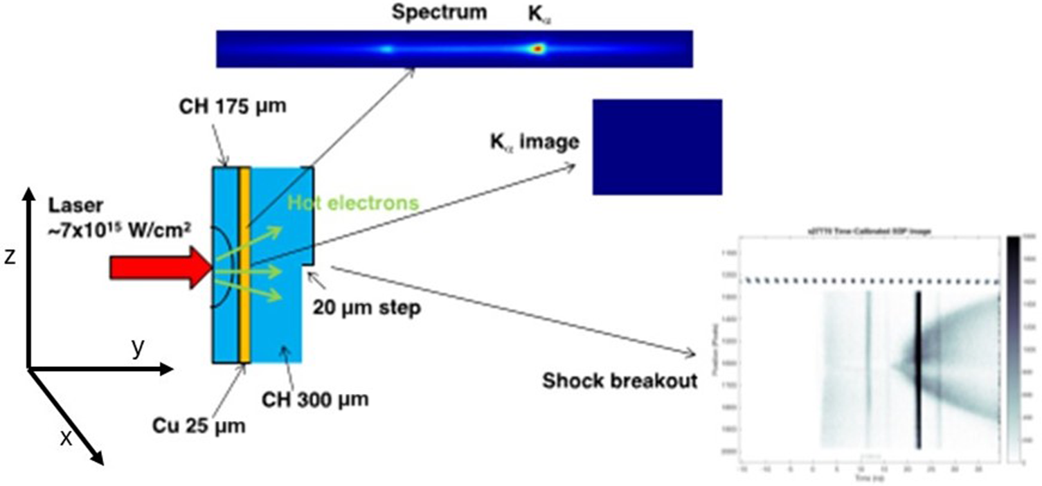
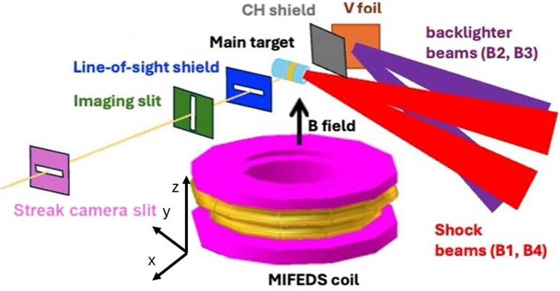
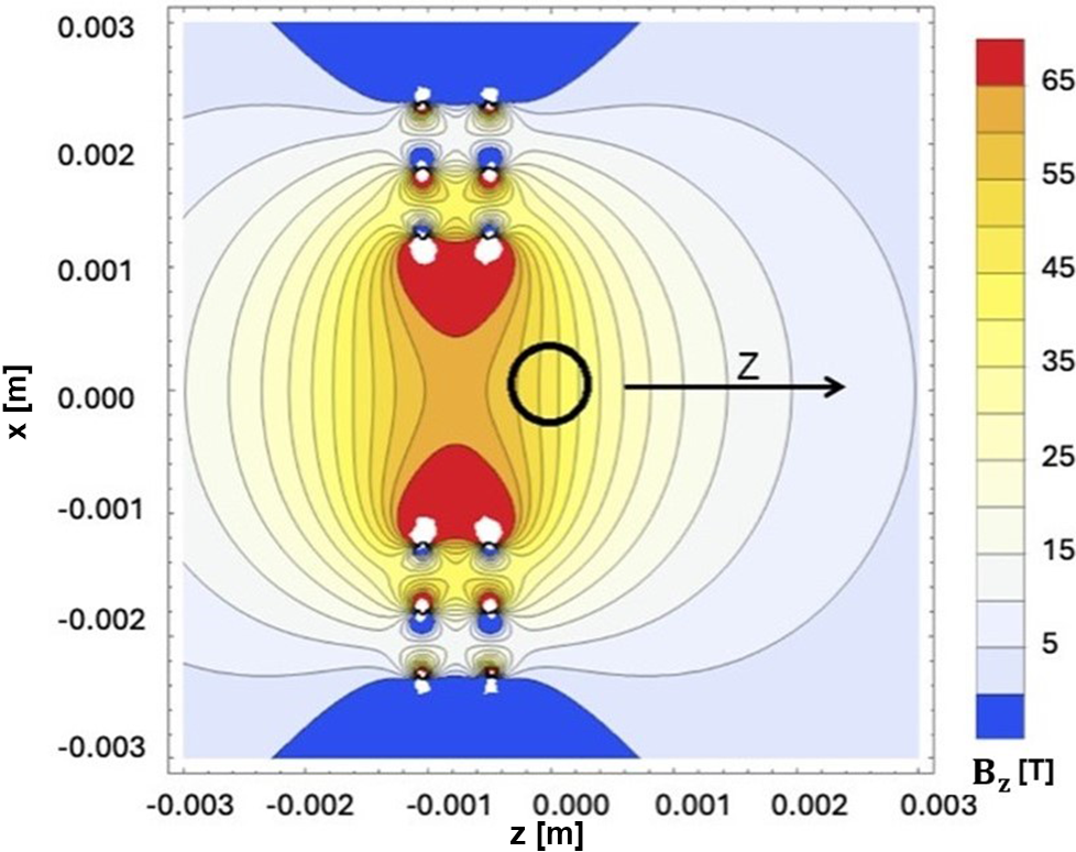
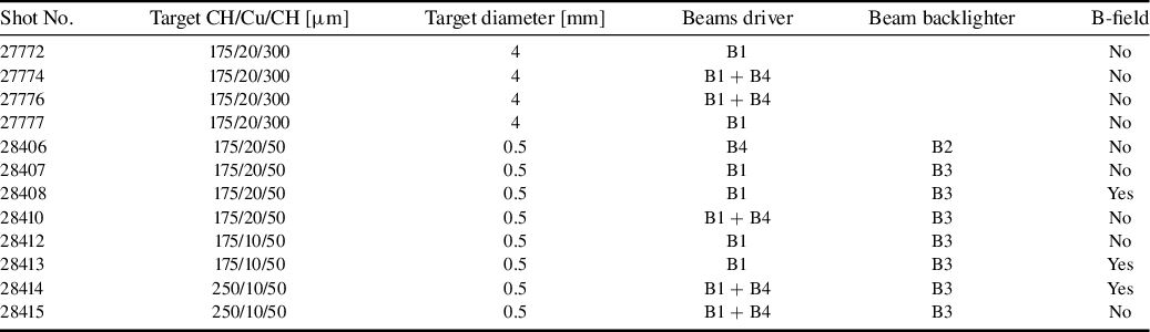
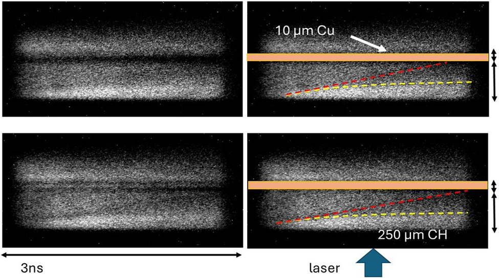
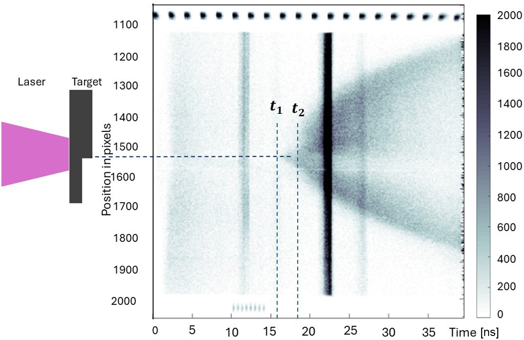
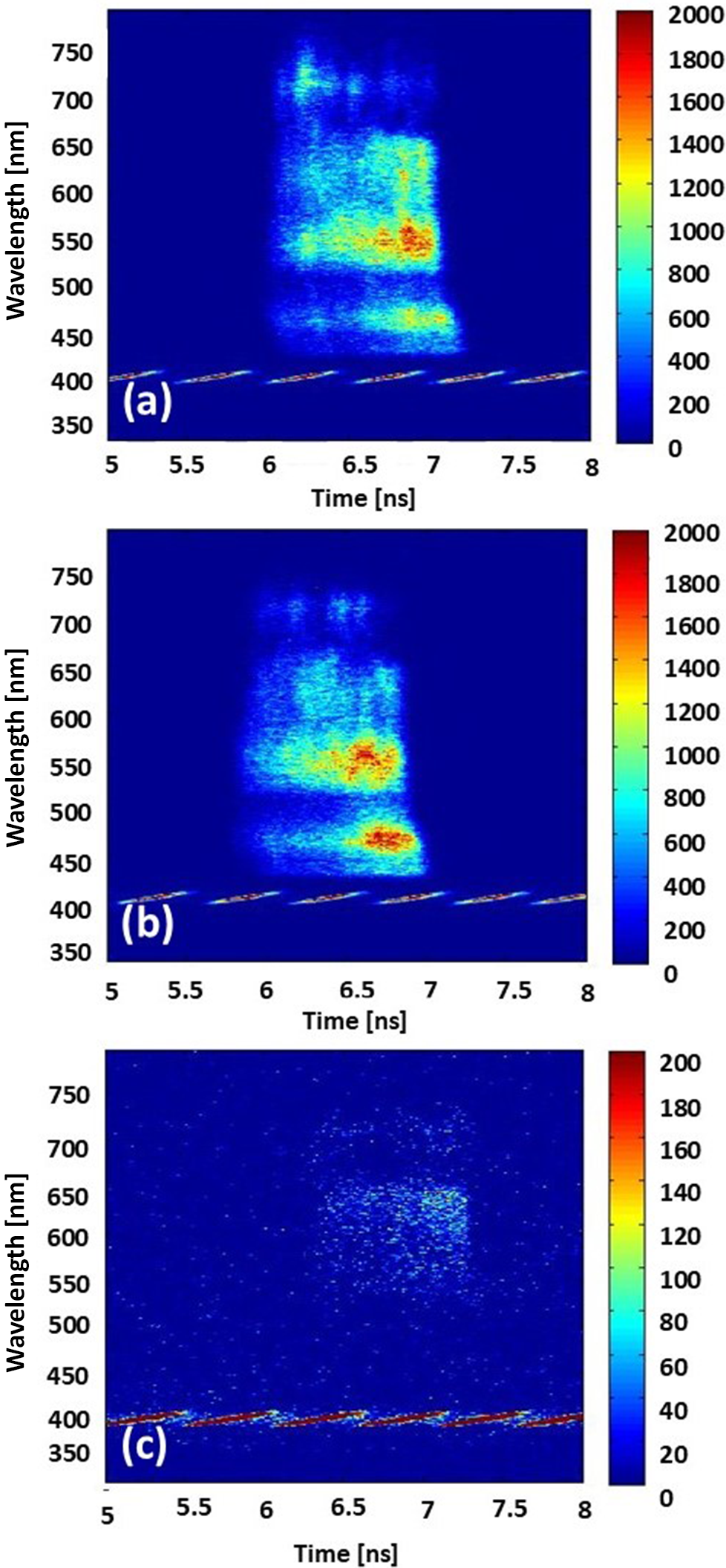
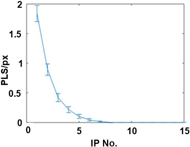
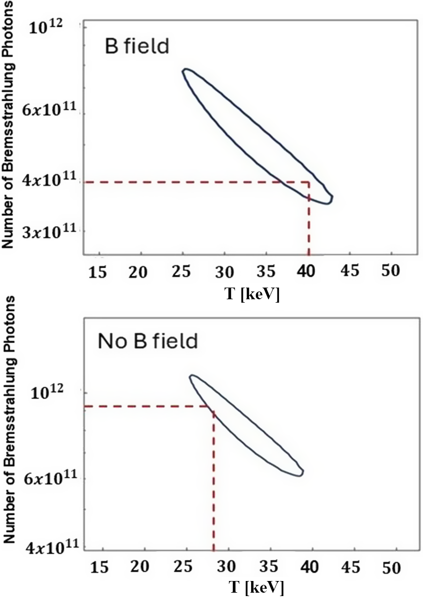


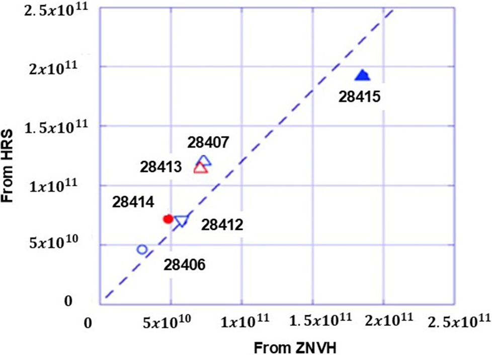

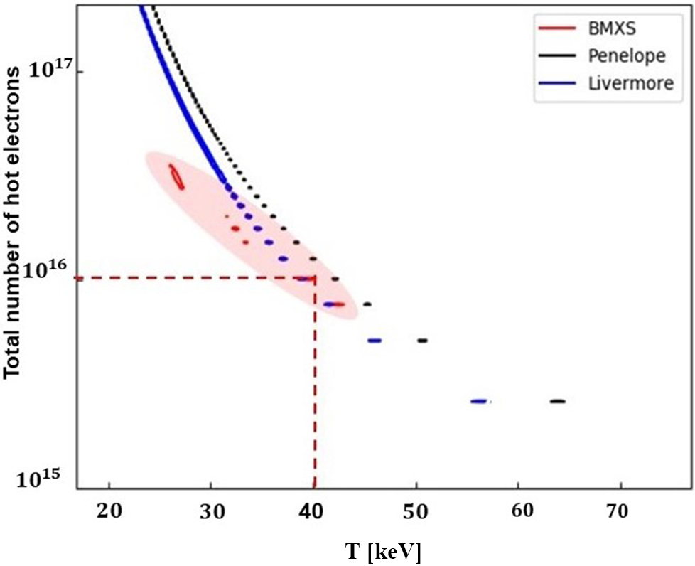

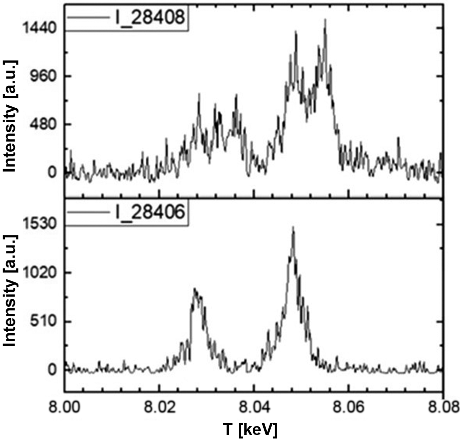

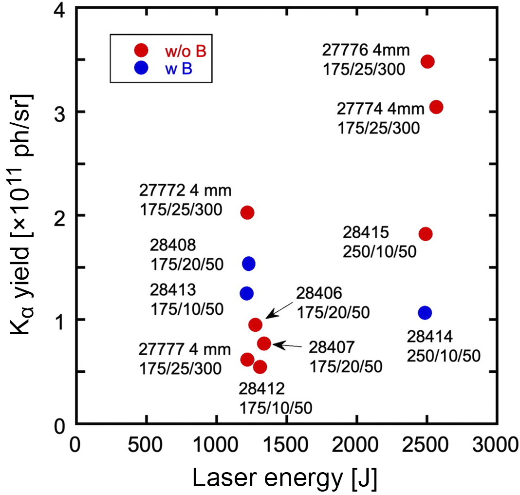

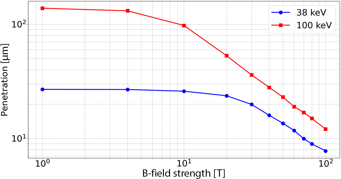

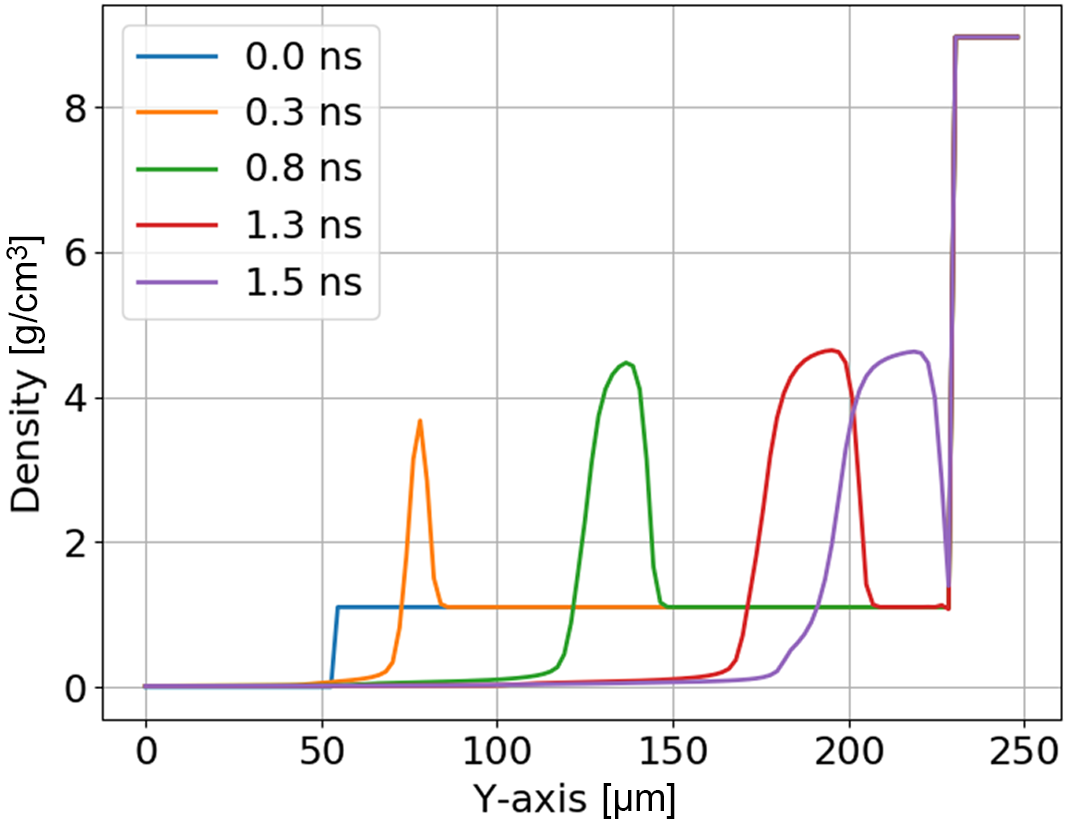
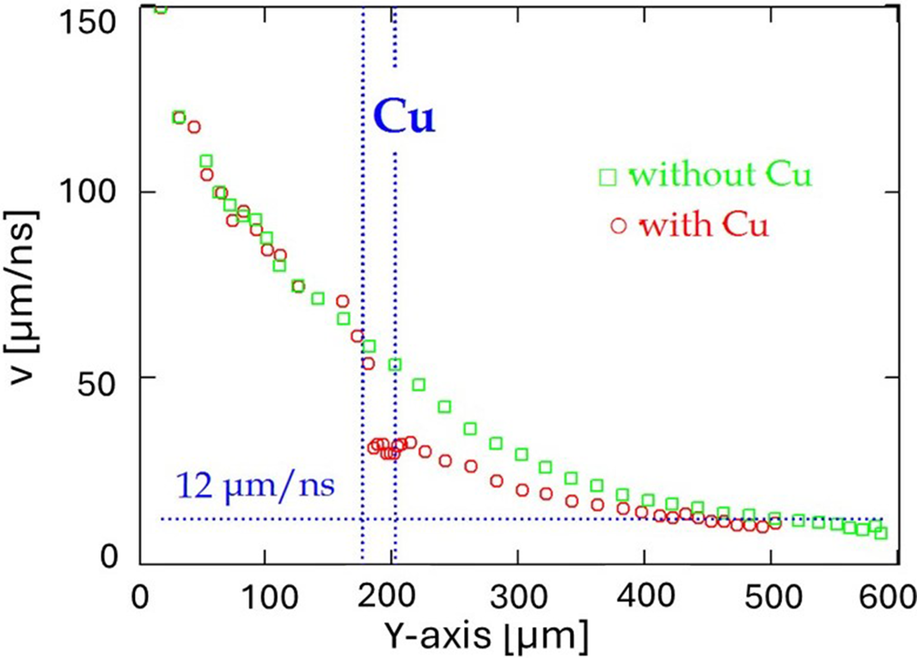
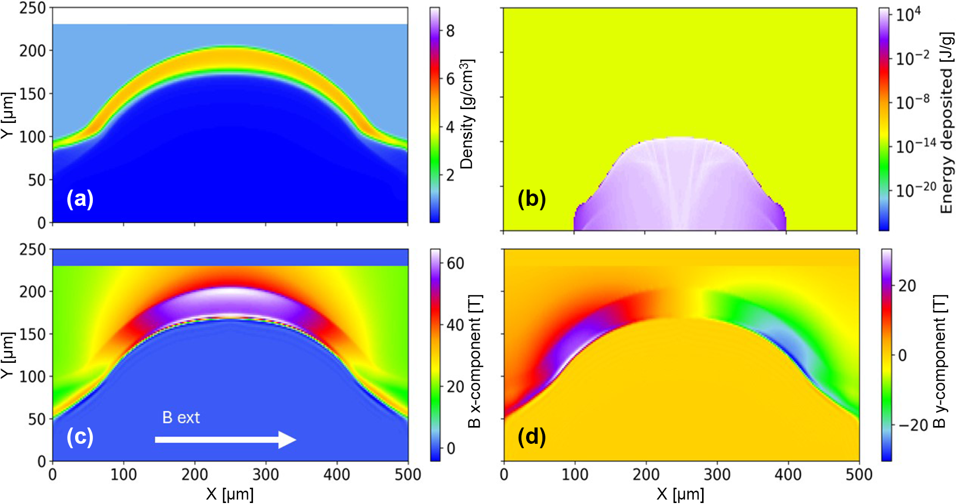


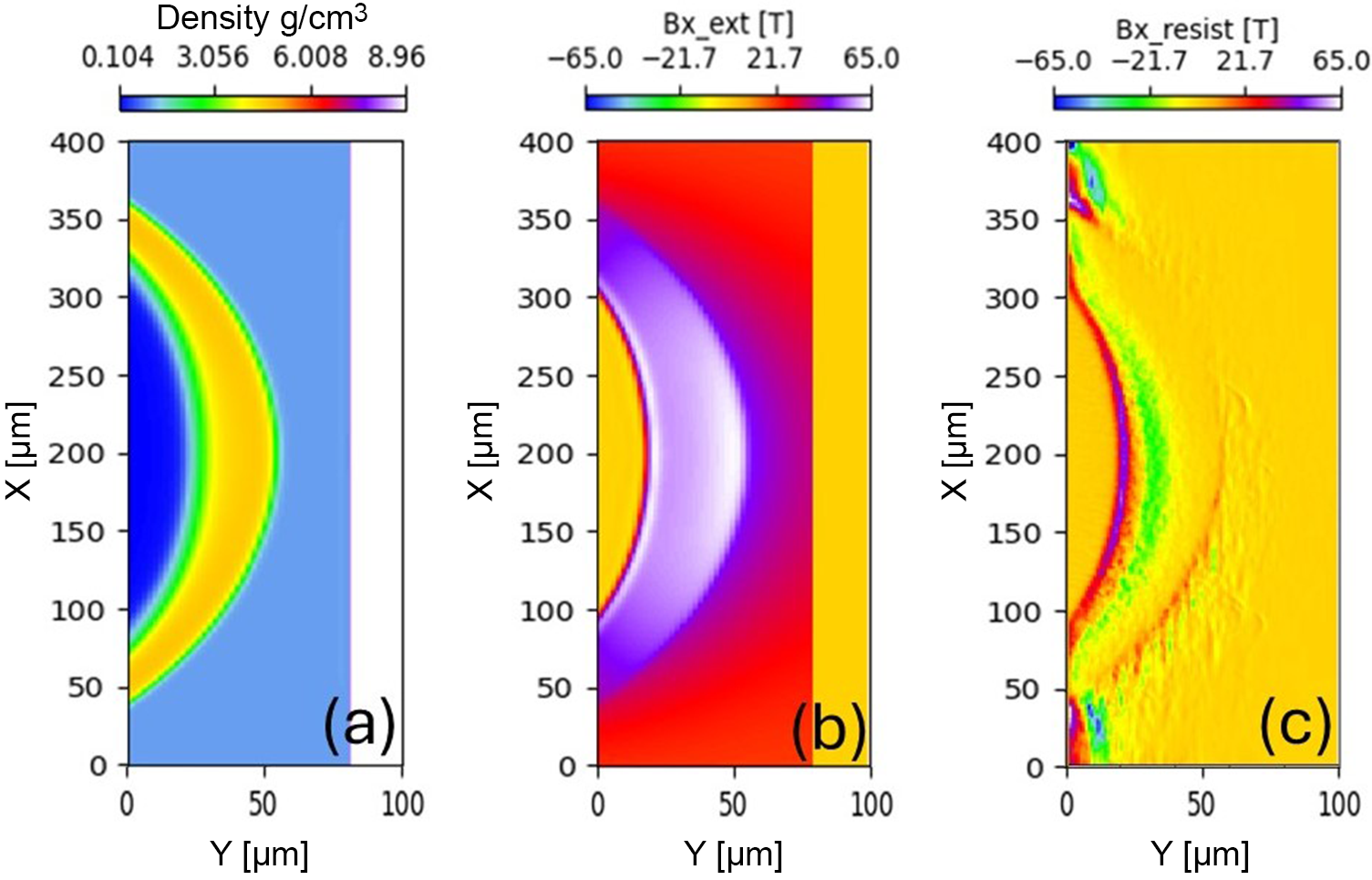


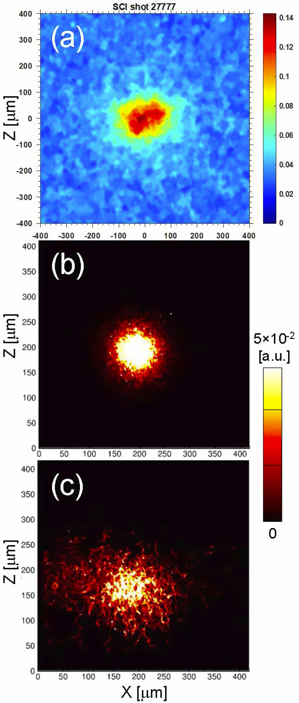


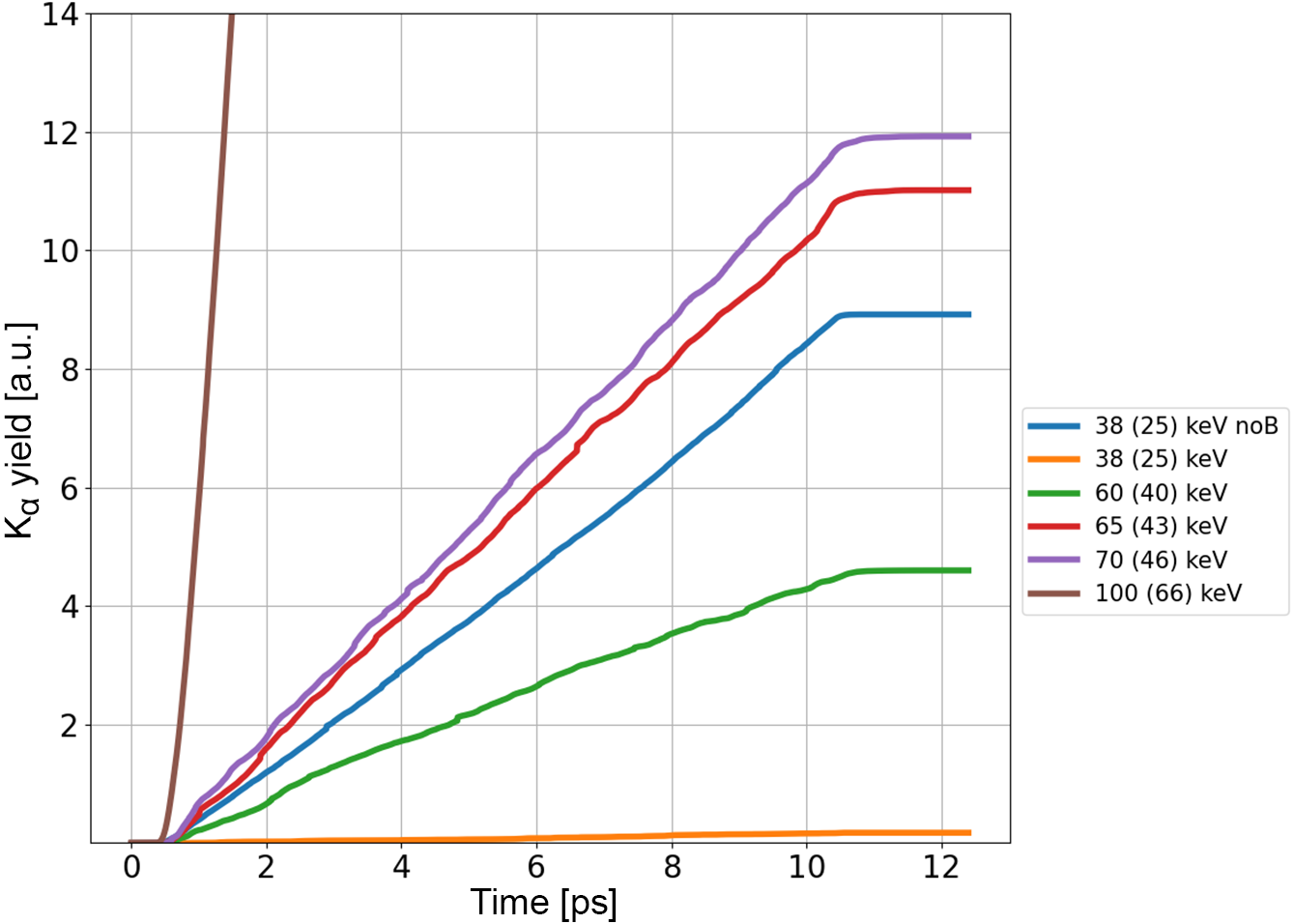


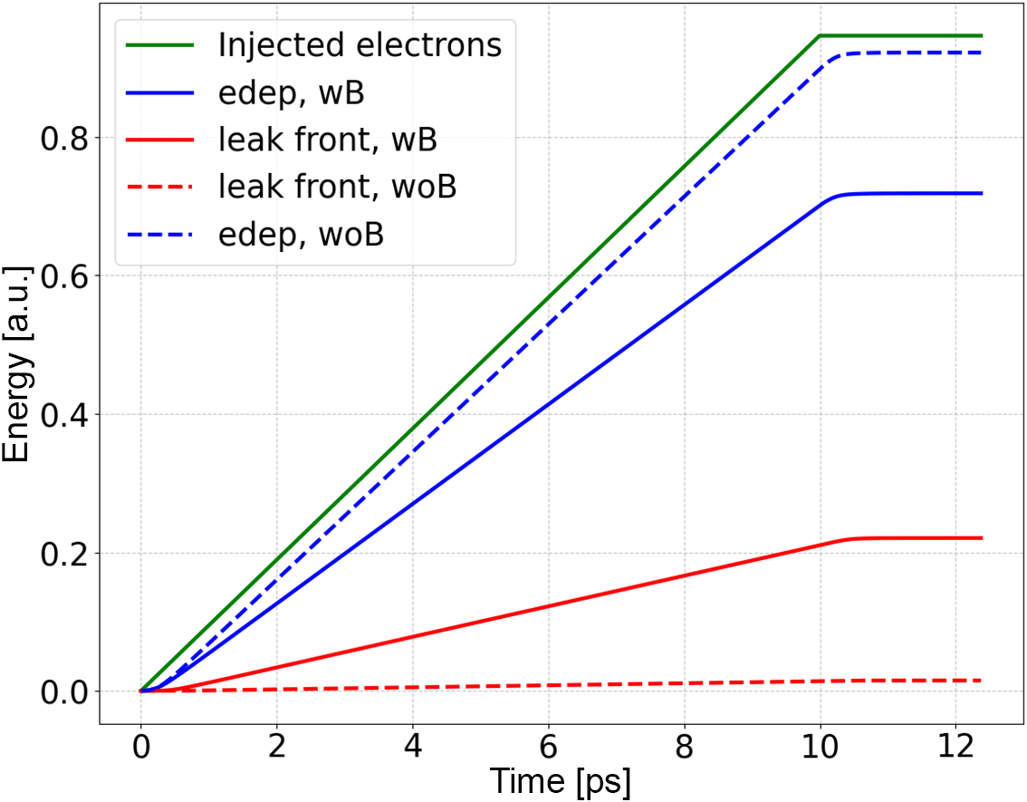


 Open access

