2. Background information

We work in Euclidean space ℝ^d, with scalar product 〈·, ·〉 and induced norm ‖ · ‖. Let B^d denote the unit ball and S^{d −1} its boundary, the unit sphere. A convex body K ⊂ ℝ^d is a nonempty compact convex set, 𝒦^d denotes the space of convex bodies together with the Hausdorff metric. We write $\mathcal{K}^d_0$ for the set of all K ∈ 𝒦^d whose Steiner point is the origin; see [Reference Schneider7] and [Reference Schneider and Weil8, Chapter 14] for further details. On 𝒦^d various geometric functionals are defined. The intrinsic volumes V _j: 𝒦^d → [0, ∞) for j = 0, …, d are positively homogeneous of degree j, motion invariant, continuous, and additive functionals, which can be introduced via the Steiner formula for the volume V _d(K + λB^d) of the parallel body K + λB^d of a convex body K ∈ 𝒦^d for λ ≥ 0. Since additivity (the valuation property) is a fundamental property which is crucial for many relations used in the following, we recall that a functional φ : 𝒦^d → ℝ is additive (a valuation) if

$$\varphi(K\cup M)+\varphi(K\cap M)=\varphi(K)+\varphi(M)$$

for all K, M ∈ 𝒦^d for which K ∪ M ∈ 𝒦^d. Moreover, as usual, we extend the domain of φ by requiring that φ(∅) = 0. The intrinsic volumes can also be viewed as particular examples of mixed volumes of convex bodies. Mixed volumes are continuous functionals V : (𝒦^d)^d → [0, ∞) which arise as coefficients in an expansion

$$V_d\bigg(\sum_{i=1}^m\lambda_iK_i\bigg)= \sum_{i_1,\ldots,i_d=1}^m\lambda_{i_1}\cdots\lambda_{i_d}V(K_{i_1}, \ldots,K_{i_d})$$

for λ _i ≥ 0 and K _i ∈ 𝒦^d, i = 1, …, m. The mixed volume is symmetric in its d arguments and, hence, uniquely determined by this expansion. Therefore, writing briefly V(K[j], M[d− j]) for V(K, …, K, M, …, M) with j copies of K and d − j copies of M, we obtain

$$V_d(K+\lambda M)=\sum_{j=0}^d\lambda^{d-j}\binom{d}{j}V(K[\,j],M[d-j])$$

for λ ≥ 0 and K ∈ 𝒦^d. In the special case j = 1 (and, similarly, for j = d − 1), as pointed out before, we have the integral representation

$$V(K[1],M[d-1])=\frac{1}{d}\int_{S^{d-1}}h(K,u)\, S_{d-1}(M,{\rm d} u),$$

where h(K, ·) is the support function of K (considered as a function on S^{d −1}) and S _d−1(M, ·) is a finite Borel measure on the unit sphere (the top-order area measure of M). Since S _d−1(M, ·) is centred (that is, the centre of the mass distribution is the origin), the integrand is only determined up to a linear function, that is, up to a translate of K. Hence, this translate can be chosen such that the Steiner point is the origin (see (1.6)).

An important result for area measures is Minkowski’s existence and uniqueness theorem (see [Reference Schneider7, Section 8.2]), which states that, for any finite, centred, and nondegenerate (not concentrated on a great subsphere) Borel measure μ on the unit sphere, there is up to a translation a unique convex body B _μ such that μ = S _d−1(B _μ, ·).

It is well known that the area measure S _d−1(K, ·) of a convex body K ∈ 𝒦^d is one member of the family of area measures S _j(K, ·), j = 0, …, d − 1, which are all finite, centred Borel measures on S^{d −1} and can be obtained via a local Steiner formula. In fact, they are all special instances of the mixed area measures (see [Reference Schneider and Weil8, Section 14.3, p. 611]). Here, however, we need another extension of the area measures that has recently been studied more intensively. First, we use the renormalization $\Psi_{d-1}(K,\cdot)\,{:\!=}\,\tfrac{1}{2}S_{d-1}(K,\cdot)$, whose total measure equals V _d−1(K). For k ∈ {1, …, d}, we then consider the flag space

$$F(d,k)\,{:\!=}\,\{(u,U)\in S^{d-1}\times G(d,k)\colon u\in U\}$$

and, on the Borel sets of F(d, j + 1), for j = 0, …, d − 1, the flag measure

(2.1)$$\begin{equation}\label{flag}\psi_j(K,\cdot)\,{:\!=}\,\int_{G(d,j+1)}\int_{S^{d-1}\cap U}\mathbf{1}\{(u,U)\in\cdot\}\, \Psi_j^U(K\mid U,{\rm d} u)\, \nu_{j+1}({\rm d} U),\end{equation}$$

where 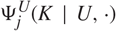$\Psi_j^U(K\mid U,\cdot)$ is the renormalized area measure of the projection of K to U, with respect to the subspace U, and ν _j+1 is the rotation invariant Haar probability measure on G(d, j + 1). In particular, the map K ↦ ψ _j(K, ·) is additive and positively homogeneous of degree j. Moreover, the measure-valued map K ↦ ψ _j(K, ·) is continuous with respect to the Hausdorff metric on 𝒦^d and the weak topology on the space of finite Borel measures on the unit sphere. This follows from (2.1) and the continuity of the area measures (and of the projection map). Observing that $\Psi_j^U(K\mid U,\cdot)=\tfrac{1}{2}S_j^U(K\mid U,\cdot)$ on S^{d −1} ∩ U and combining (4.78), (4.11), and (4.9) from [Reference Schneider7] (in this order), we obtain

(2.2)$$\begin{equation}\label{totalmass} \psi_j(K,F(d,j+1))=\frac{\Gamma({d}/{2})\Gamma({1}/{2})} {\Gamma({(j+1)}/{2})\Gamma({(d-j)}/{2})} \binom{d-1}{j}^{-1} V_j(K). \end{equation}$$

We refer the reader to [Reference Hug, Türk, Weil and Ludwig6] for background information on flag measures of convex bodies (in particular, for different normalizations and isomorphic versions), and to [Reference Hug, Rataj and Weil4] and [Reference Hug, Rataj and Weil5] for integral representations of mixed volumes and mixed functionals with respect to flag measures as needed here and described in the following sections.

In addition to the mixed volumes, we need certain mixed functionals of translative integral geometry and their relation to mixed volumes. The mixed functionals we will make use of are determined by the iterated translative integral formula for the intrinsic volumes. Defining V _j(∅) = 0, we obtain

$$\begin{align*}&\int_{{\rm R}^d}\dots\int_{{\rm R}^d}V_j(K_1\cap (K_2+x_2)\cap\cdots\cap (K_k+x_k))\, \lambda_d({\rm d} x_2)\cdots \lambda_d({\rm d} x_k) \\ & \qquad =\sum_{\substack{m_1,\ldots,m_k=\,j\\m_1+\cdots+m_k=(k-1)d+j}}^{d}V_{m_1,\ldots,m_k}(K_1,\ldots,K_k)\end{align*}$$

for j ∈ {0, …, d}, k ≥ 2, and K ₁, … , K _k ∈ 𝒦^d. Here λ _d denotes the d-dimensional Lebesgue measure. We refer the reader to [Reference Schneider7], [Reference Schneider and Weil8], and [Reference Schulte, Weil, Vedel Jensen and Kiderlen9] for properties of the mixed functionals $V_{{m_1},\ldots,{m_k}}$ and various (local and abstract) extensions. As mentioned in the introduction, mixed volumes and the mixed functionals of translative integral geometry are different objects, but they are closely related for k = 2 and j = 0 where we have

(2.3)$$\begin{equation}\label{eqrel} \binom{d}{m}V(K[m],M[{d-m}])=V_{m,d-m}(K,M^*). \end{equation}$$

The mixed functionals again satisfy translative integral geometric formulae. In the following, the value of a functional which is evaluated at the empty set (in one argument) is defined to be 0. Using this, we have

$$\begin{align*} &\int_{{\mathbb R}^d}V_{m_1,\ldots,m_{k-2},m}(K_1,\ldots,K_{k-2},K_{k-1}\cap (K_k+x))\,\lambda_d({\rm d} x) \\ &\qquad=\sum_{\substack{m_{k-1}\!,m_k=m\\m_{k-1}+m_k=d+m}}^{d} V_{m_1,\ldots,m_{k-2},m_{k-1}\!,m_k}(K_1,\ldots,K_{k-2},K_{k-1},K_k) \end{align*}$$

for k ≥ 3 and m ₁ + · · · + m _k−2 + m = (k − 2)d + j.

These functionals on convex bodies and their additive extensions to polyconvex sets are used in the study of Boolean models. In the introduction a stationary Boolean model Z was defined as the union set of a stationary Poisson particle process X in 𝒦^d. Here we can think of X as a random collection of particles or as a (almost surely simple) random counting measure (we prefer the latter point of view). An alternative description of a Boolean model in terms of an independently marked Poisson point process is given in [Reference Schneider and Weil8] (see also the extensive literature cited therein). Writing 𝔼 for the expectation with respect to an underlying probability measure ℙ, we assume in the following that the intensity measure 𝔼X of X is locally finite and nonzero, and, hence, by stationarity, has the form

$$\mathbb{E} X(\cdot)=\gamma\int_{\mathcal{K}^d_0}\int_{{\rm R}^d}\mathbf{1} \{K+x\in\cdot\}\,\lambda_d({\rm d} x)\,\mathbb{Q}({\rm d} K),$$

where γ ∈ (0, ∞) is the intensity of X and ℚ is a probability measure on the space of convex bodies, concentrated on bodies with Steiner point at the origin. Assuming that the intensity measure 𝔼X is locally finite is equivalent to requiring that

(2.4)$$\begin{equation}\label{locfinBM} \int_{\mathcal{K}^d_0}V_j(K)\, \mathbb{Q}({\rm d} K)<\infty,\qquad j=1,\ldots,d, \end{equation}$$

and ensures that indeed Z is a random closed set. This assumption is always tacitly made. For our analysis, we will need the additional moment assumption

(2.5)$$\begin{equation}\label{moment} \int_{\mathcal{K}^d_0}V_1(K)^{d-2}\, \mathbb{Q}({\rm d} K)<\infty , \end{equation}$$

which implies (2.4) for j = 1, …, d − 2, by a special case of [Reference Schneider and Weil8, Equation (14.31)] and Hölder’s inequality. In particular, all moments with exponent j < d − 2 are finite as well. If φ is a measurable, nonnegative functional on (𝒦^d)^q+r which is translation invariant in each argument, we define the mean values of φ for the particle process X by

$$\begin{align&#x002A;} \overline\varphi(X,\ldots,X,M_1,&\ldots ,M_r) \,{:\!=}\,\gamma^q\int_{(\mathcal{K}^d_0)^{q}}\varphi(K_1,\ldots,K_q,M_1, \ldots, M_r)\, \mathbb{Q}^q({\rm d}(K_1,\ldots,K_q)) \end{align&#x002A;}$$

for M ₁, … , M _r ∈ 𝒦^d. Here we allow r = 0, which defines $\overline\varphi(X,\ldots,X)$. Thus, in particular, the mean values V̅ _j(X), V̅_m(X, …, X), and V̅ _m,d−j(X, …, X, M) from the introduction are defined and finite, as a consequence of (2.4) and the translative integral formula. In addition to scalar-valued mean values, the mean values of support functions and area measures are also required. They are defined in the obvious way by

$$\overline{h}(X,\cdot)\,{:\!=}\,\gamma\int_{\mathcal{K}^d_0} h(K,\cdot)\, \mathbb{Q}({\rm d} K)$$

and

$$\overline{S}_{d-1}(X,\cdot)\,{:\!=}\,\gamma\int_{\mathcal{K}^d_0} S_{d-1}(K,\cdot)\,\mathbb{Q}({\rm d} K).$$

It follows from (2.4) that h̅(X, ·) is a finite function, which is again a support function of a convex body $M(X)\in {\cal K}^d_0$, the mean body of X, and S̅ _d−1(X, ·) is again a finite, centred Borel measure on the unit sphere. If it is nondegenerate then it is the area measure of a convex body $B(X)\in {\cal K}^d_0$, the Blaschke body of X, which is determined by

$$\overline{S}_{d-1}(X,\cdot)=S_{d-1}(B(X),\cdot).$$

It is important to keep in mind that these mean values and B(X) are deterministic objects, and X simply reminds us of the dependence on X, that is, on γ and ℚ, which are uniquely determined by X. Furthermore, (2.2) and (2.4) imply that the mean flag measures of X are finite measures.

The Blaschke body B(X) of X exists, if the measure S̅ _d−1(X, ·) is not supported by a subsphere of S^{d −1}. This means that the distribution ℚ is not concentrated on convex bodies which all lie in parallel hyperplanes. We can and will assume this without loss of generality, since in a Boolean model with particles lying in parallel hyperplanes almost surely no overlaps occur. Thus, in this case the intensity of X can be estimated directly since the Boolean model Z and the particle process X contain the same information. In particular, Theorem 1.1 trivially holds in this case.

Under the given assumptions, the additivity properties of the functionals V _j and V( · [j], K[d − j]) also ensure that the deterministic densities (specific mean values) V̅ _j(Z) and V̅(Z[j], K[d− j]) of the Boolean model Z can be defined. One possibility would be to use the relations to the mean values of X, as they were described in the introduction, relations which are specific for the current setting that is based on an underlying Poisson process. However, such densities can be defined for functionals φ of more general random sets Z, either through a limit for a sequence of growing windows (which requires the additivity of φ) or as a Radon– Nikodym derivative, which is based on local versions of the functionals φ. We refer the reader to [Reference Schneider and Weil8, Chapter 9] for details.

3. The four-dimensional case

We now complete the proof of Theorem 1.1 in the case where d = 4. It motivates the ideas for the general case in the next section, but is simpler and, therefore, shorter due to the structure of the (specific) mixed mean values which occur. We first recall the density formulae for the mixed volumes in four dimensions. They read

(3.1)$$\begin{align} \overline V_4(Z) &=1-{\rm e}^{-\overline V_4(X)},\label{4-4} \end{align} $$

(3.2)$$\begin{align} \overline V(Z[3],K[1]) &={\rm e}^{-\overline V_4(X)}\overline V(X[3],K[1]), \label{4-3} \end{align} $$

(3.3)$$\begin{align} \overline V(Z[2],K[2]) &={\rm e}^{-\overline V_4(X)}\big(\overline V(X[2],K[2]) -\tfrac{1}{12}\overline V_{3,3,2}(X,X,K^&#x002A;)\big),\label{4-2} \end{align}$$

(3.4)$$\begin{align} \overline V(Z[1],K[3]) &={\rm e}^{-\overline V_4(X)}\big(\overline V(X[1],K[3]) -\tfrac{1}{4}\overline V_{2,3,3}(X,X,K^&#x002A;)\nonumber\\ &\qquad +\tfrac{1}{24}\overline V_{3,3,3,3}(X,X,X,K^&#x002A;)\big),\label{4-1} \end{align} $$

(3.5)$$\begin{align}\overline V_0(Z) &={\rm e}^{-\overline V_4(X)}\big( \overline V_0(X) -\overline V_{1,3}(X,X) -\tfrac{1}{2}\overline V_{2,2}(X,X) + \tfrac{1}{2}\overline V_{2,3,3}(X,X,X)\\ & \qquad -\tfrac{1}{24}\overline V_{3,3,3,3}(X,X,X,X)\big).\end{align}$$

This is the corrected version of [Reference Weil11, Equation (20)], both with respect to the missing term V̅ _2,2(X, X) and to erroneous constants. We assume that all five specific mean values on the left-hand sides of (3.1)–(3.5) are known for all K. Clearly, (3.1) determines the factor e^{−V̅ ₄(X)} in all other equations. From (1.6) we thus find that (3.2) determines the mean area measure S̅ ₃(X, ·) and, thus, the Blaschke body B(X). In [Reference Weil11, Proposition 3], it was shown that in all mean values, where the homogeneity index 3 occurs, the corresponding variable X can be replaced by B(X). For example,

$$\overline V_{3,3,2}(X,X,K^&#x002A;) = V_{3,3,2}(B(X),B(X),K^&#x002A;),$$

which is determined since B(X) is known. Thus, (3.3) yields

$$\overline V(X[2],K[2]) = \tfrac{1}{6}\overline V_{2,2}(X,K^&#x002A;)\quad\text{for all $K$. }$$

Using the translative integral formula for the variable K, we obtain the mean mixed functional V̅ _2,3,3(X, K, M) for all convex bodies K and M. In fact, for all convex bodies 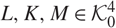$L,K,M\in\mathcal{K}^4_0$ and α, β ≥ 0, we have

$$\begin{align&#x002A;} &\int_{{\mathbb R}^4} V_{2,2}(L,(\alpha K)\cap (\beta M+x))\, \lambda_4({\rm d} x) \\ &\quad =\alpha^2\beta^4 V_{2,2}(L,K)V_4(M)+\alpha^4\beta^2 V_{2,2}(L,M)V_4(K) +\alpha^3\beta^3V_{2,3,3}(L,K,M), \end{align&#x002A;}$$

and, hence,

$$\begin{align&#x002A;} &\int_{{\mathbb R}^4} \overline{V}_{2,2}(X,(\alpha K)\cap (\beta M+x))\, \lambda_4({\rm d} x) \\ &\qquad=\alpha^2\beta^4 \overline{V}_{2,2}(X,K)V_4(M) + \alpha^4\beta^2 \overline{V}_{2,2}(X,M)V_4(K) +\alpha^3\beta^3\overline{V}_{2,3,3}(X,K,M). \end{align&#x002A;}$$

In particular, we obtain the quantities

$$\overline V_{2,3,3}(X,B(X),K^&#x002A;)= \overline V_{2,3,3}(X,X,K^&#x002A;)$$

in (3.4) and

$$\overline V_{2,3,3}(X,B(X),B(X))= V_{2,3,3}(X,X,X)$$

in (3.5). Thus, from (3.4), V̅(X[Reference Alesker1], K[Reference Hug and Rataj3]) is determined for all K. Again by (1.6), this gives ̅h(X, ·) and, hence,

$$\overline V_{1,3}(X,X) = \int_{S^{3}} \overline h(X,-u)\,\overline S_3(X,{\rm d} u) .$$

Therefore, the only summand in (3.5) which remains to be discussed (apart from γ = V̅ ₀(X)) is V̅ _2,2(X, X). As we will show, this mean value is determined by the knowledge of V̅(X[Reference Goodey and Weil2], K[Reference Goodey and Weil2]) for all K, which we have already obtained.

For a continuous function g on the flag space F(4, 3), we consider the continuous functional φ _g: 𝒦^d → ℝ which is defined by

$$\varphi_g (M) = \int_{F(4,3)} g(u,L)\,\psi_2(M,{\rm d} (u,L)),\qquad M\in {\cal K}^d,$$

and its mean value

$$\overline\varphi_g (X) = \gamma\int_{{\cal K}^d_0} \varphi_g (M)\,{\mathbb Q}({\rm d} M) = \int_{F(4,3)} g(u,L)\, \overline\psi_2(X,{\rm d} (u,L)).$$

Obviously, φ _g is an element of ${\bf Val}_2^{(4)}$, the vector space of translation invariant, continuous valuations on ℝ⁴ which are positively homogeneous of degree 2. By Alesker’s result [Reference Alesker1], φ _g can be approximated by linear combinations of special mixed volumes, that is, for each ε > 0, there are n ∈ ℕ, λ ₁, …, λ _n ∈ ℝ, and 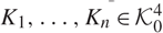$K_1,\ldots,K_n\in\mathcal{K}^4_0$ such that

$$|\varphi_g(M)-\sum_{i=1}^n\lambda_i V(M[2], K_i[2])|\le\varepsilon R(M)^2\le \varepsilon V_1(M)^2$$

for all M ∈ 𝒦^d where R(M) denotes the circumradius of M and where we used the inequalities V ₁(M) ≥ diam(M) ≥ R(M). The latter follows since V ₁ is an increasing functional, homogeneous of degree 1, V ₁(I) = 1 if I is a segment of length 1, and the centre of the circumball of M is contained in M. Hence,

$$|\overline \varphi_g(X)-\sum_{i=1}^n\lambda_i \overline V(X[2], K_i[2])|\le \varepsilon c,$$

with some constant c ≥ 0, due to assumption (2.5) for d = 4. This shows that $\overline \varphi_g(X)$ is determined by V̅(X[Reference Goodey and Weil2], K[Reference Goodey and Weil2]) for all $K\in\mathcal{K}^4_0$. Note that the mean value $\overline \varphi_g(X)$ exists, since (2.2) yields

$$\int_{F(4,3)} |g(u,L)|\,\overline\psi_2(X,{\rm d} (u,L)) \le \|g\| \overline V_2(X)<\infty ,$$

where ‖ g ‖ denotes the maximum norm of g (and the constant in (2.2) is $\smash{\tfrac23}$ for d = 4 and j = 2). Thus, we obtain $\int_{F(4,3)} g(u,L)\,\overline\psi_2(X,{\rm d}(u,L))$ for all continuous functions g, and therefore $\overline\psi_2(X,\cdot)$. But then $\overline\psi_2(X^&#x002A;,\cdot)$ is also determined.

Again let ε > 0 be arbitrary. In [Reference Hug, Rataj and Weil4], an ε-approximation V ^(ε)(M[2], K*[2]) ≥ 0 of the mixed volume V(M[2], K*[2]) for any $M,K\in\mathcal{K}^4_0$ has been introduced such that

$$V^{(\varepsilon)}(M[2],K^&#x002A;[2])\nearrow V (M[2],K^&#x002A;[2]) \quad\text{as $\varepsilon\searrow 0$. }$$

Moreover, it was shown that there exist bounded, measurable functions $f_2^{(\varepsilon)}$ on F(4, 3) × F(4, 3) such that

$$\begin{align&#x002A;} V^{(\varepsilon)}(M[2],K^&#x002A;[2]) =\int_{F(4,3)}\int_{F(4,3)} f_2^{(\varepsilon)} (u,L,u',L')\,\psi_2(K^&#x002A;,{\rm d}(u',L'))\,\psi_2(M,{\rm d}(u,L)). \end{align&#x002A;}$$

Integration against γ ²ℚ² then yields

(3.6)$$\begin{align} &\int_{F(4,3)}\int_{F(4,3)} f_2^{(\varepsilon)} (u,L,u',L')\,\overline\psi_2(X^&#x002A;,{\rm d}(u',L'))\,\overline\psi_2(X,{\rm d}(u,L)) \nonumber \\ &\quad =\gamma^2 \int_{\mathcal{K}^4_0}\int_{\mathcal{K}^4_0}V^{(\varepsilon)}(M[2],K^&#x002A;[2])\, \mathbb{Q}({\rm d} K)\,\mathbb{Q}({\rm d} M)\nonumber \\ &\quad \nearrow \gamma^2 \int_{\mathcal{K}^4_0}\int_{\mathcal{K}^4_0}V (M[2],K^&#x002A;[2])\, \mathbb{Q}({\rm d} K)\, \mathbb{Q}({\rm d} M)\nonumber \\ &\quad =\overline V (X[2],X^&#x002A;[2])\label{intmean} \end{align}$$

as ε ↘ 0. Since $\overline\psi_2(X,\cdot)$ and $\overline\psi_2(X^&#x002A;,\cdot)$ are determined, we finally conclude that 6V̅(X[Reference Goodey and Weil2], X*[Reference Goodey and Weil2]) = V _2,2(X, X) is determined as well. This completes the proof of the four-dimensional case of Theorem 1.1 and replaces the incomplete proof in [Reference Weil11].

4. Proof of the general case

For general dimension d ≥ 5, more complicated mixed functionals and their (specific) mean values occur, which cannot be expressed by the Blaschke body and the mean body anymore. Here, we need the recent extension [Reference Hug, Rataj and Weil5] of the flag formulae. Moreover, the truncation argument which we used already in the previous section is more subtle and will be explained in detail.

To start with the proof of Theorem 1.1, we again use the facts that V̅ _d(Z) and the equation

$$\overline V_d(Z) = 1-{\rm e}^{-\overline V_d(X)}$$

determine the factor

$$q= {\rm e}^{-\overline V_d(X)}$$

in the remaining equations. Thus,

$$\overline V(Z [d-1], K[1]) = q\,\overline V(X [d-1],K [1])$$

determines V̅(X[d – 1], K[1] for all K ∈ 𝒦^d. It follows from (1.6) that this determines the mean area measure S̅ _d−1(X, ·). Up to a constant, this is the mean flag measure $\overline \psi_{d-1}(X,\cdot)$ (if we identify (u, ℝ^d) and u). We now proceed by recursion.

Proposition 4.1

Let j ∈ {1, …, d − 2}, and assume that q and the mean flag measures $\overline\psi_{d-1}(X,\cdot),\dots,\overline\psi_{j+1}(X,\cdot) $ are given. Then the values of the densities V̅(Z[j], K[d − j]) for all K ∈ 𝒦^d determine the mean flag measure $\overline \psi_j(X,\cdot)$.

Proof. We recall (1.4) in the more explicit form

(4.1)$$\begin{align} &\binom{d}{j}\overline V(Z [j], K[d-j] ) \\ &\qquad = q \Biggl(\binom{d}{j}\overline V(X [j], K[d-j] ) \\ &- \sum_{k=2}^{d-j} \frac{(-1)^k}{k!} \sum_{\substack{m_1,\ldots ,m_k=j+1\\ m_1+\cdots + m_k=(k-1)d+j}}^{d-1} \overline V_{m_1,\dots,m_k,d-j}(X,\dots,X, K^&#x002A;)\Biggr).\label{nonisotropic2} \end{align}$$

In [Reference Hug, Rataj and Weil5, Section 6] the formula

(4.2)$$\begin{align}\label{genflagform} &V_{\boldsymbol m}(K_1,\dots ,K_k,K^&#x002A;)\nonumber \\ &\qquad = \int_{F(d,d-j+1)}\int_{F(d,m_k+1)}\cdots \int_{F(d,m_1+1)}f_{\boldsymbol m}(u_1,L_1,\dots ,u_k,L_k,u,L)\nonumber \\ & \times \,\psi_{m_1}(K_1,{\rm d}(u_1,L_1))\cdots \\ &\times\psi_{m_k}(K_k,{\rm d}(u_k,L_k))\,\psi_{d-j}(K^&#x002A;,{\rm d}(u,L)) \end{align}$$

was proved. Here, the index m stands for (m ₁, …, m_k, d − j) and the function f_m is of the form

$$f_{\boldsymbol m}(u_1,L_1,\dots ,u_k,L_k,u,L) = G_{\boldsymbol m}(u_1,\dots ,u_k,u)\cdot \phi_{\boldsymbol m}(u_1,L_1,\dots ,u_k,L_k,u,L).$$

Also, G_m ≥ 0 is measurable, but unbounded, whereas ϕ_m is a signed continuous function. Both functions are given explicitly in [Reference Hug, Rataj and Weil5]. The special case in which k = 1 was treated in [Reference Hug, Rataj and Weil4] and has been used in the previous section for dimension d = 4. In this generality the formula requires that the bodies K ₁, …, K _k, K ^* are in general position. We need not go into details here, since we will use an argument to avoid this condition. Namely, we consider, as in [Reference Hug, Rataj and Weil5], the bounded approximation

$$V_{\boldsymbol m}^{(\varepsilon)}(K_1,\dots ,K_k,K^&#x002A;)\ge 0,\qquad \varepsilon > 0,$$

which can be described similarly as in (4.2), but with a function $f_{\boldsymbol m}^{(\varepsilon)}$ which is obtained by replacing G_m(u ₁, …, u _k, u) by the bounded, measurable, and nonnegative function

$$G_{\boldsymbol m}^{(\varepsilon)}(u_1,\dots ,u_k,u) = G_{\boldsymbol m}(u_1,\dots ,u_k,u){\bf 1}\{\operatorname{dist}(o,\text{conv}\{ u_1,\dots ,u_k,u\})\ge \varepsilon\} ,$$

where conv {u ₁, …, u _k, u} denotes the convex hull of u ₁, …, u _k, u ∈ ℝ^d. Since (by definition) G_m(u ₁, …, u _k, u) = 0 if u ₁, …, u _k, u are linearly dependent, we obtain

$$G_{\boldsymbol m}^{(\varepsilon)} \nearrow G_{\boldsymbol m} \quad\text{as $\varepsilon \searrow 0$.}$$

As was shown in [Reference Hug, Rataj and Weil5, Section 6], this implies that

$$V_{\boldsymbol m}^{(\varepsilon)}(K_1,\dots ,K_k,K^&#x002A;)\nearrow V_{\boldsymbol m}(K_1,\dots ,K_k,K^&#x002A;)$$

for all K ₁, … , K _k, K ∈ 𝒦^d, without an additional condition of general position. The reason is that V_m(K ₁, …, K _k, K ^*) obeys a curvature representation over the normal bundles of the bodies K ₁, …, K _k, K ^* (this was shown in [Reference Hug and Rataj3]), and the truncated functional $V_{\boldsymbol m}^{(\varepsilon)}(K_1,\dots ,K_k,K^&#x002A;)$ has a similar representation (this was shown in [Reference Hug, Rataj and Weil5]).

Now we can proceed with the proof. The definition of the truncated functionals and the monotone convergence transfers to the mean values

$$\begin{align&#x002A;} &\overline V_{\boldsymbol m}^{(\varepsilon)}(X,\dots ,X,K^&#x002A;) \\ &\quad = \int_{F(d,d-j+1)}\int_{F(d,m_k+1)}\cdots \int_{F(d,m_1+1)}f_{\boldsymbol m}^{(\varepsilon)}(u_1,L_1,\dots ,u_k,L_k,u,L)\nonumber \\ & \times \overline\psi_{m_1}(X,{\rm d}(u_1,L_1))\cdots \\ & \times \overline\psi_{m_k}(X,{\rm d}(u_k,L_k))\, \psi_{d-j}(K^&#x002A;,{\rm d}(u,L)) \end{align&#x002A;}$$

and

$$\begin{align&#x002A;}\\[-24pt] \overline V_{\boldsymbol m}^{(\varepsilon)}(X,\dots ,X,K^&#x002A;) & =\gamma^k \int V_{\boldsymbol m}^{(\varepsilon)}(K_1,\dots ,K_k,K^&#x002A;)\, \mathbb{Q}^k({\rm d}(K_1,\ldots,K_k)) \\ & \nearrow \gamma^k \int V_{\boldsymbol m} (K_1,\dots ,K_k,K^&#x002A;)\, \mathbb{Q}^k({\rm d}(K_1,\ldots,K_k)) \\ & =\overline V_{\boldsymbol m}(X,\dots ,X,K^&#x002A;) \end{align&#x002A;}$$

as ε ↘ 0, compare the derivation of (3.6). Due to our assumptions, the mean flag measures $\overline\psi_{m_1}(X,\cdot),\dots,$ $\overline\psi_{m_k}(X,\cdot)$ are determined (recall that m _i ≥ j + 1), and, thus, $\overline V_{\boldsymbol m}^{(\varepsilon)}(X,\dots ,X,K^&#x002A;)$ is determined for all ε > 0, which gives V̅_m(X, …, X, K ^*) for all K. From (4.1), we deduce that V̅(X[j], K[d − j]) is given for all K.

In the remaining part of the proof, we argue as in the four-dimensional case. Let φ _g be a valuation of the form

$$\varphi_g (M) = \int_{F(d,j+1)} g(u,L)\,\psi_j(M,{\rm d}(u,L)),$$

where M ∈ 𝒦^d and g is a continuous function on F(d, j + 1). Any such valuation is translation invariant, continuous, and homogeneous of degree j. From Alesker’s result it follows that, for each ε > 0, there are n ∈ ℕ, λ₁, …, λ_n ∈ ℝ, and K ₁, … , K _n ∈ 𝒦^d such that

$$\bigg|\varphi_g(M)-\sum_{i=1}^n\lambda_i V(M[j],K_i [d-j])\bigg|\le \varepsilon V_1(M)^j \quad\text{for all $M\in\mathcal{K}^d$. }$$

Hence, under the moment assumption (2.5), we conclude that the mean values $\overline\varphi_g (X)$ are determined. The corresponding integrals then determine $\overline\psi_j(X,\cdot )$.

To complete the proof of Theorem 1.1, we note that we already obtained the mean values q = e^{−V̅ _d(X)} and $\overline \psi_{d-1}(X,\cdot)$, the starting point for the recursion. Proposition 4.1 thus shows that all mean flag measures

$$\overline \psi_{d-1}(X,\cdot),\dots , \overline \psi_{1}(X,\cdot)$$

are determined. Using (4.2) again, together with the truncation method explained above, we obtain all mean values

$$\overline V_{m_1,\dots, m_k}(X,\dots,X)$$

with m _i ∈ {1, …, d − 1} and such that m ₁ + · · · + m_k = (k − 1)d.

By (1.5), the intensity γ is determined.

6. Nonstationary Boolean models

In [Reference Weil11] (see also [Reference Schneider and Weil8, Section 11.1]) (1.2)–(1.4) were generalized to certain nonstationary Boolean models Z, namely those for which the underlying Poisson process X has a translation regular intensity measure Θ. This condition means that Θ is absolutely continuous with respect to a translation-invariant, locally finite measure $\tilde\Theta$ on 𝒦^d. Explicitly, we have

(6.1)$$\begin{equation}\label{transregular} \Theta (A) = \int_{{\cal K}^d_0}\int_{{\rm R}^d} {\bf 1}_A(K+x)\eta(K,x)\,\lambda_d({\rm d} x)\,{\mathbb Q}({\rm d} K) \end{equation}$$

for all Borel sets A ⊂ 𝒦^d and with a measurable function η ≥ 0 on ${\cal K}^d_0\times{\rm R}^d$. In order to simplify the following presentation, we make the additional assumption that η is continuous and does not depend on K, that is, η(x) is the spatial intensity of X at x ∈ ℝ^d. We call such a Boolean model regular. Under these conditions, the decomposition (6.1) is unique and the densities of mixed volumes and mixed functionals in the following formulae exist pointwise (not only almost everywhere). The counterpart to (1.2)–(1.4) is given by the system

(6.2)$$\begin{align} \overline V_d(Z;\,z) &= 1-{\rm e}^{-\overline V_d(X;\,z)} ,\label{vol} \end{align} $$

(6.3)$$\begin{align} \overline V(Z [d-1], K[1];\,z) &= {\rm e}^{-\overline V_d(X;\,z)}\overline V(X [d-1],K [1];\,z) ,\label{surf} \end{align}$$

and

(6.4)$$\begin{align}\\[-24pt]\label{nonstationary} &\binom{d}{j}\overline V(Z [j], K[d-j];\,z ) \nonumber \\ &\qquad ={\rm e}^{-\overline V_d(X;z)} \sum_{{\boldsymbol m}\in\operatorname{mix}(j)} \frac{(\!-1)^{{|{\boldsymbol m}|}-1}}{|{\boldsymbol m}|!}\overline V_{{\boldsymbol m},d-j}(X,\dots,X, K^&#x002A;;\,z,\dots ,z), \end{align}$$

for j = 0, …, d − 2, all z ∈ ℝ^d, and all K ∈ 𝒦^d. Here, on the left-hand side of (6.2), the function V̅ _d(Z; ·) is defined as the Radon–Nikodym derivative of the expectation measure 𝔼λ_d(Z, .) (where λ_d(Z, ·) denotes the restriction of the Lebesgue measure λ_d to Z). Similarly, $\binom{d}{j}\overline V(Z [j], K[d-j];\cdot )$ for j = 0, …, d − 1 is defined as the Radon–Nikodym derivative of the expectation measure 𝔼Φ_j,d-j(Z, K*;· ×ℝ^d), where $\Phi_{j,d-j}(Z,K^&#x002A;;\cdot)=\Phi_{j,d-j}^{(0)}(Z,K^&#x002A;;\cdot)$ is the mixed translative measure, the local variant of the mixed functional V _j,d−j(Z, K ^*) (see [Reference Schneider and Weil8, Section 5.2]). Recall here that $\binom{d}{j}V(M[j],K[d-j]) =V_{j,d-j}(M,K^&#x002A;)$. Also, it should be mentioned that Φ_j,d−j(Z(ω), K ^*; · ×ℝ^d) exists by additive extension and is a locally finite signed measure on ℝ^d for all sets Z(ω) in the extended convex ring. Thus, the random variable Φ_j,d−j(Z, K ^*; A × ℝ^d) is defined and finite for every bounded Borel set A ⊂ ℝ^d.

On the right-hand side of (6.4), the mean mixed functionals V̅ _m,d−j(X, …, X, K ^*; ·) for m ∈ mix (j, k) are defined more directly as Radon–Nikodym derivatives of the expectation measures

(6.5)$$\begin{equation}\label{instatexp} \mathbb E\sum_{(M_1,\ldots ,M_k)\in X^k_{\not =}}\Phi_{{\boldsymbol m},d-j}(M_1,\ldots,M_k,K^&#x002A;;\cdot\times{\rm R}^d) \end{equation}$$

with respect to $\lambda_d^k$ (the k-fold product measure of λ_d). The summation here is over all k-tuples (M ₁, … , m_k) ∈ (𝒦^d)^k of pairwise different particles M _i in X, and the mixed measure Φ_m,d−j(M ₁, …, m_k, K ^*; ·) is a finite measure on (ℝ^d)^k+1 and arises from the (iterated) translative integral formula for the local analog of the intrinsic volumes, the curvature measures (see [Reference Weil11, Section 5] and [Reference Schneider and Weil8, Section 6.4]). As was shown in [Reference Weil11, Theorem 5], the measure (6.5) is indeed locally finite and absolutely continuous. Moreover, the derivative satisfies

(6.6)$$\begin{align}\label{derivative} &\overline V_{{\boldsymbol m},d-j}(X,\dots,X, K^&#x002A;;\,z_1,\ldots, z_k) \nonumber \\ &\qquad = \int_{({\cal K}_0^d)^k}\int_{({\mathbb R}^d)^k}\eta(z_1-x_1)\cdots\eta(z_k-x_k)\nonumber \\ & \times\Phi_{{\boldsymbol m},d-j}(M_1,\ldots,M_k,K^&#x002A;;\,{\rm d}(x_1,\ldots ,x_k)\times{{\mathbb R}}^d)\,\mathbb Q^k({\rm d}(M_1,\ldots ,M_k)) . \end{align}$$

Since we require η to be continuous, this integral representation in fact holds for all (z ₁, …, z _k) ∈ (ℝ^d)^k, not only almost everywhere. The explicit form of the density V̅(Z[j], K[d − j];· ×ℝ^d) was determined in [Reference Weil11, Theorem 6] (see also [Reference Schneider and Weil8, Theorem 11.1.2]). Here, in lines 10–13 of the proof [Reference Weil11, p. 54], the differential λ_d(dz ₁) · · · λ_d(dz _k) has to be replaced by λ_d(dz) and, consequently, the variables z ₁, …, z _k in the integrands have to be replaced by one variable z.

Since, for j = 0, the decomposition result, which we used for mixed volumes and mixed functionals, also holds for the mixed measures in (6.6), we obtain from (6.4) the following formula for the density of the Euler characteristic at z ∈ ℝ^d:

(6.7)$$\begin{align}\label{nonstationaryEuler} \overline V_0(Z;\,z ) &={\rm e}^{-\overline V_d(X;\,z)} \sum_{{\boldsymbol m}\in\operatorname{mix}(0)} \frac{(-1)^{{|{\boldsymbol m}|}-1}}{|{\boldsymbol m}|!}\overline V_{{\boldsymbol m}}(X,\dots,X;\,z,\dots ,z). \end{align}$$

In order to discuss the question which information on X can be extracted from the local densities of Z in (6.4), let us start with the simpler equations (6.2) and (6.3). Obviously, (6.2) determines q(z) : = e^{−V̅ _d(X;z)} and, given q(z), (6.3) determines the mean mixed volume V̅(X[d − 1], K[1];z) for all K ∈ 𝒦^d. From (6.6) we obtain

$$\begin{align&#x002A;} d\overline V(X [d-1],K [1];z) = \int_{{\cal K}_0^d}\int_{{\rm R}^d}\eta(z-x)\, \Phi_{d-1,1}(M,K^&#x002A;;\,{\rm d} x\times{{\mathbb R}}^d)\,\mathbb Q({\rm d} M), \end{align&#x002A;}$$

and [Reference Goodey and Weil2, Corollary 3] yields

$$\begin{align&#x002A;} d\overline V(X [d-1],K [1];z) &= \int_{{\cal K}_0^d}\int_{{\rm Nor} (M)} \eta(z-x)h^&#x002A;(K,u)\,\Theta_{d-1}(M;\,{\rm d} (x,u))\,\mathbb Q({\rm d} M) \\ &= \int_{S^{d-1}} h^&#x002A;(K,u)\, \mu_z({\rm d} u) , \end{align&#x002A;}$$

where μ _z is the measure

$$\mu_z (\cdot)\,{:\!=}\, \int_{{\cal K}_0^d}\int_{{\rm Nor} (M)}\eta(z-x){\bf 1} (u\in\cdot)\,\Theta_{d-1}(M,{\rm d} (x,u))\,\mathbb Q({\rm d} M)$$

on S^{d −1} and Θ_d−1(M, ·) is the (d − 1)th support measure (normalized as in [Reference Schneider7]) on the normal bundle Nor (M) of M. If we write ω _d−1 for the spherical Lebesgue measure and center μ _z by

$$\mu_z^&#x002A; (\cdot)\,{:\!=}\, \mu_z(\cdot) - \frac{1}{\kappa_d}\int_{S^{d-1}} {\bf 1}(u\in\cdot)\langle u,c\rangle\,\omega_{d-1}({\rm d} u),$$

with

$$c\,{:\!=}\, \int_{S^{d-1}} u\, \mu_z({\rm d} u),$$

then the collection of densities V̅(X[d − 1], K[1];z), K ∈ 𝒦^d, determines $\mu_z^&#x002A;$ uniquely (see [Reference Goodey and Weil2, Lemma 4]).

This observation already emphasizes a difficulty which arises for nonstationary Z. Namely, mixed volumes are translation invariant in each component. Therefore, they provide information only on the bodies involved which are of ‘centred type’ (surface area measures, flag measures, centred support functions, etc.). Consequently, in the nonstationary case, a centredness property of the Boolean model Z seems necessary. Let us assume, for fixed z ∈ ℝ^d, that Z is centred at z, meaning that c = 0 (that is, μ _z is centred) or, equivalently, $\mu_z^&#x002A; = \mu_z$. A simple sufficient condition which ensures that μ _z is centred is that η is symmetric with respect to z, that is, η(z − x) = η(z + x) for all x ∈ ℝ^d, and that ℚ is symmetric with respect to reflection in the origin, in the sense that $\mathbb{Q}^&#x002A;\,{:\!=}\,\mathbb{Q}(\{M\in\mathcal{K}^d_0\,\colon\, M^&#x002A;\in\cdot\})=\mathbb{Q}$. This follows from

$$\begin{align&#x002A;} &\int_{{\cal K}_0^d}\int_{{\rm Nor} (M)}\eta(z-x)u\,\Theta_{d-1} (M,{\rm d} (x,u))\,\mathbb Q({\rm d} M) \\ &\qquad = \int_{{\cal K}_0^d}\int_{{\rm Nor} (M^&#x002A;)}\eta(z-x)u\,\Theta_{d-1}(M^&#x002A;,{\rm d}(x,u))\,\mathbb Q({\rm d} M) \\ &\qquad = -\int_{{\cal K}_0^d}\int_{{\rm Nor} (M)}\eta(z+x)u\,\Theta_{d-1}(M,{\rm d}(x,u))\,\mathbb Q({\rm d} M), \end{align&#x002A;}$$

where we used the rotation covariance of Θ_d−1(M, ·) for the last equality.

In dimensions 2 and 3, and for a Boolean model Z which is centred at z, we obtain uniqueness theorems similar to our Theorem 1.1. The case in which d = 2 was discussed in [Reference Weil10] (and again in [Reference Goodey and Weil2]) and the case in which d = 3 in [Reference Goodey and Weil2]. It was shown that the local densities V̅(Z[j], K[d − 1];z) for j = 0, …, d and all K ∈ 𝒦^d determine the convoluted intensity function

$$\overline V_0(X;z) \,{:\!=}\, \int_{{\rm R}^d} \eta (z-x)\,\tilde\Phi_0(X,{\rm d} x),$$

where

$$\tilde\Phi_0(X,\cdot)\, \,{:\!=}\, \int_{{\cal K}_0^d} \Phi_0(M,\cdot)\,\mathbb Q({\rm d} M)$$

is the expected (with respect to ℚ ) Gaussian curvature measure of the particles. If Z is stationary then η ≡ γ ; hence, V̅ ₀(X;z) = γ since Φ₀(M, ℝ^d) = V ₀(M) = 1. Note that these results are of local type, they hold for a fixed position z ∈ ℝ^d, and require only the knowledge of the local densities of Z in z. Since in [Reference Goodey and Weil2] and [Reference Weil10] there were some erroneous statements about the centredness of certain functions, we sketch the proofs of these results here. As explained above, we obtain q(z) and $\mu_z^&#x002A;$. Then, for d = 2, only (6.7) remains, reading

$$\begin{align&#x002A;} \overline V_0(Z;\,z ) &=q(z)\big(\overline V_0(X;\,z) - \tfrac{1}{2}\overline V_{1,1}(X,X;z,z)\big). \end{align&#x002A;}$$

As was shown in [Reference Goodey and Weil2] (combine page 332, lines -1 to -3, and Corollary 2),

$$\overline V_{1,1}(X,X;z,z) = \int_{S^1}\int_{S^1} \alpha (u,v) |\det (u,v)|\,\mu_z({\rm d} u)\,\mu_z({\rm d} u),$$

where α(u, v) ∈ [0, π] is the angle between u and v, and | det (u, v)| is the absolute determinant. For centred Z, $\mu_z=\mu_z^&#x002A;$ is known, which gives V̅ _1,1(X, X;z, z) and, thus, V̅ ₀(X;z).

For d = 3, we have two remaining equations,

$$\overline V(Z[1],K[2];z ) =q(z)\tfrac{1}{3}\big(\overline V_{1,2}(X,K^&#x002A;;z) - \tfrac{1}{2}\overline V_{2,2,2}(X,X,K^&#x002A;;z,z)\big)$$

and

$$\overline V_0(Z;z ) =q(z)\big(\overline V_0(X;z) - \overline V_{1,2}(X,X;z,z)+\tfrac{1}{6}\overline V_{2,2,2}(X,X,X;z,z,z)\big).$$

Concerning the first equation, it was shown in [Reference Goodey and Weil2, p. 342] that

$$\begin{align&#x002A;} \overline V_{2,2,2}&(X,X,K^&#x002A;;z,z) = \int_{S^2}\int_{S^2} \int_{S^2}\alpha (u,v,w)|\det (u,v,w)|\,\mu_z({\rm d} u)\,\mu_z({\rm d} v)\,S_2(K^&#x002A;,{\rm d} w), \end{align&#x002A;}$$

where α(u, v, w) is now a spherical angle between u, v, w (the spherical volume of the spherical triangle spanned by these vectors) and | det (u, v, w)| is the absolute determinant. Again, using the fact that Z is centred and, hence, that $\mu_z=\mu_z^&#x002A;$ is known, we obtain V̅ _1,2(X, K ^*;z). Letting K vary, Lemma 5 of [Reference Goodey and Weil2] shows that $h_z^&#x002A;$ is determined for d = 3. Here,

$$h_z(u) \,{:\!=}\, \int_{{\cal K}_0^d}\int_{{\rm R}^d}\eta(z-x)\,\rho(M;u,{\rm d} x)\,\mathbb Q({\rm d} M),\qquad u\in S^{d-1},$$

is the density of the support function of X, defined via the local version of the support function h(M, ·), the support kernel ρ(M;·, dx), and $h_z^&#x002A;$ is the centred version

$$h_z^&#x002A;(\cdot) \,{:\!=}\, h_z(\cdot) - \frac{1}{\kappa_d}\Big\langle\cdot\,, \int_{S^{d-1}} uh_z(u)\,\omega_{d-1}({\rm d} u)\Big\rangle.$$

From [Reference Weil11, p. 343] we get

$$\overline V_{2,2,2}(X,X,X;z,z,z) = \int_{S^2}\int_{S^2} \int_{S^2}\alpha (u,v,w) |\det (u,v,w)|\,\mu_z({\rm d} u)\,\mu_z({\rm d} v)\,\mu_z({\rm d} w).$$

Using [Reference Weil11, p. 344], we obtain

$$\begin{align&#x002A;} \overline V_{1,2}(X,X;z,z) &= \int_{S^2} h_z(\!-u)\,\mu_z({\rm d} u)= \int_{S^2} h_z^&#x002A;(-u)\,\mu_z^&#x002A;({\rm d} v), \end{align&#x002A;}$$

where we used the fact that $\mu_z=\mu_z^&#x002A;$ is centred (by assumption). This finally shows that V ₀(X;z) is determined. We emphasize that the assumption that $h_z=h_z^&#x002A;$ is not necessary for this argument (and also not sufficient, in contrast to a claim in [Reference Goodey and Weil2]).

In these small dimensions 2 and 3, spherical quantities like the measure μ _z and the function h _z, as well as their centred versions are sufficient for integral representations of the mean mixed functionals which occur in (6.4). If we look at the proof of Theorem 1.1 for d ≥ 4 it combines two fundamental steps which would be essential in the nonstationary case also. The first is the use of flag measures to obtain a corresponding integral representation of the mean mixed functionals of X. This step can in fact also be made for the local mixed densities in (6.6), using a local flag representation of the mixed curvature measures Φ_m,d−j(M ₁, …, m_k, K ^*; · ) proved in [Reference Hug, Rataj and Weil5, Theorem 5] (and based on a recent result in [Reference Hug and Rataj3]). Since (6.6) depends on the location z ∈ ℝ^d, a more general flag measure is involved, the flag support measure θ _j(K, ·). The latter is a finite Borel measure on the extended flag space ℝ^d × F(d, j + 1) which, in extension of (2.1), is defined by

$$\theta_j(K,\cdot)=\int_{G(d,j+1)}\int_{S^{d-1}\cap U}\mathbf{1} \{(x,u,U)\in\cdot\}\, \Theta_j^U(K\mid U,{\rm d}(x,u))\, \nu_{j+1}({\rm d} U).$$

Here, 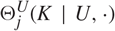$\Theta_j^U(K\mid U,\cdot)$ is the jth support measure of the projection of K onto U, calculated in the subspace U. For properties, different normalizations and isomorphic versions of support measures and their flag versions, we refer the reader to [Reference Hug, Türk, Weil and Ludwig6] and [Reference Schneider7].

The second essential step in the proof of Theorem 1.1 was to proceed from the mean mixed volumes V̅(X[j], K[d − j]) for K ∈ 𝒦^d to the mean flag measure $\overline\psi_j(X,\cdot)$ for the next round of the recursion. This step was based on Alesker’s approximation of translation-invariant, continuous valuations on 𝒦^d by linear combinations of mixed volumes. In the nonstationary case, in each recursion step, we would obtain the local density

$$\begin{align&#x002A;} \overline V(X [j],K [d-j];z) = \int_{{\cal K}_0^d}\int_{{\mathbb R}^d}\eta(z-x)\,\Phi_{j,d-j}(M,K^&#x002A;;\,{\rm d} x\times{{\mathbb R}}^d)\,\mathbb Q({\rm d} M), \end{align&#x002A;}$$

and would need to show that these densities, given for all K ∈ 𝒦^d (and a fixed z ∈ ℝ^d), determine the convoluted mean flag support measure

$$\mu_{z,j}(\cdot)\,{:\!=}\,\int_{{\cal K}^d_0}\int_{{\mathbb R}^d\times F(d,j+1)}\eta(z-x) {\bf 1}((u,L)\in\cdot )\, \theta_j(M,{\rm d}(x,u,L))\,\mathbb Q({\rm d} M),$$

respectively its centred version $ \mu_{z,j}^&#x002A;$. Here, Alesker’s theorem does not seem applicable, since the dependence on z (and, thus, the occurrence of x in the flag measure) does not allow us to define an appropriate valuation which is translation invariant. It is also likely that further centredness conditions like $\mu_{z,j}=\mu_{z,j}^&#x002A;$ are needed for such a step.