

1. Introduction
Lipid bilayer membranes are fascinating systems from multiple scientific perspectives. Biologically (Alberts et al. Reference Alberts, Bray, Lewis, Raff, Roberts and Watson1994; Gennis, Reference Gennis1989; Lodish et al. Reference Lodish, Baltimore, Berk, Zipursky, Matsudaira and Darnell1995), membranes are among the most important and most versatile components of biological cells; biomembranes protect cells from their surroundings, provide a means to compartmentalize subcellular function and act as a scaffolding for countless biochemical reactions involving membrane-associated proteins. Membranes accomplish all this while being sufficiently flexible to allow the cell to grow, move and deform as necessary to allow the cell to perform its duties as part of a larger organism. The use of lipid-bilayer membranes in pharmaceutical and related technological applications is also prevalent and growing (Evans & Wennerstrom, Reference Evans and Wennerstrom1994; Immordino et al. Reference Immordino, Dosio and Cattel2006; Tien & Ottova-Leitmannova, Reference Tien and Ottova-Leitmannova2003).
From the physical perspective, lipid-bilayer membranes are no less fascinating (Lipowsky & Sackmann, Reference Lipowsky and Sackmann1995; Nelson et al. Reference Nelson, Piran and Weinberg2004). Membranes provide a naturally occurring experimental realization for a two-dimensional (2D) (actually, ‘quasi-2D’ (Oppenheimer & Diamant, Reference Oppenheimer and Diamant2009)) fluid. In vivo, biomembranes contain a wide assortment of molecules (multiple lipid species, proteins, cholesterol, etc.), which by elementary thermodynamic considerations (Gibbs phase rule (Callen, Reference Callen1961)) would be expected to produce a rich phase behavior. In fact, even single-component phospholipid bilayers in vitro can exhibit non-trivial and subtle phase behavior (Nagle, Reference Nagle1980), with binary and ternary model systems quickly becoming very complicated and often difficult to interpret unambiguously (McConnel & Vrljic, Reference McConnell and Vrljic2003; Simons & Vaz, Reference Simons and Vaz2004b). Of course, real cell membranes are not equilibrium systems, they are part of a living organism that is constantly expending energy to maintain the processes of life (Boal, Reference Boal2002; Howard, Reference Howard2001; Nelson, Reference Nelson2008). Consequently, cell membranes offer a seemingly limitless opportunity to study non-equilibrium statistical mechanics in the context of naturally occurring biological phenomena. As a single prominent example, the question of whether or not the inhomogeneity observed in the plasma membrane of living animal cells (i.e. ‘lipid rafts’ and/or ‘lipid microdomains’ (Edidin, Reference Edidin2003; Simons & Vaz, Reference Simons and Vaz2004a)) is driven by thermodynamics or active manipulation by the cell remains unanswered (Fan et al. Reference Fan, Sammalkorpi and Haataja2010). Indeed, the lipid raft hypothesis remains one of the more controversial topics in modern-day biology and biophysics.
The purpose of this review is not to speculate on the nature of lipid rafts or to discuss the many biological functions of membranes within the cell. Rather, we consider the possibility of quantitatively simulating experimental model membrane systems with the goal of understanding membrane dynamics in the mesoscopic/macroscopic length and time regimes commonly accessed by optical microscopy. The philosophy here is one of ‘learn to walk before you run’; developing the tools to quantitatively describe dynamics in well-characterized model systems seems a necessary first step on the more ambitious road toward understanding the dynamics of true biomembranes. To this end, we adopt minimalist descriptions for membrane energetics motivated by classical continuum theories (elasticity, binary mixture models, etc.) and evolve the dynamics of such systems using equations of motion that account for hydrodynamic flow and thermal fluctuations. The inclusion of hydrodynamic interactions is critical to a proper modeling of membrane dynamics; this is a primary message of this review and the examples and discussion provided herein are chosen to emphasize this point.
Our conceptual picture of biological membranes as a ‘two-dimensional oriented solution of integral proteins … in the viscous phospholipid bilayer’ (Singer & Nicolson, Reference Singer and Nicolson1972) was popularized by Singer and Nicolson well over 30 years ago. Quantitative physical models for the continuum-level energetics (Canham, Reference Canham1970; Helfrich, Reference Helfrich1973) and dynamics (Brochard & Lennon, Reference Brochard and Lennon1975) associated with shape fluctuations of homogeneous fluid membranes were developed shortly thereafter. And, Saffman and Delbruck (SD) (Saffman & Delbrück, Reference Saffman and Delbrück1975) suggested a hydrodynamic model for flow within and around the bilayer, leading to quantitative predictions for lateral diffusion coefficients of integral membrane proteins that still find widespread use up to this day (Ramadurai et al. Reference Ramadurai, Holt, Krasnikov, van den Bogaart, Killian and Poolman2009; Saxton & Jacobson, Reference Saxton and Jacobson1997). The SD hydrodynamic model has since been revisited and reformulated (Alexander et al. Reference Alexander, Bernoff, Mann, Mann, Wintersmith and Zou2007; Goldstein & Jackson, Reference Goldstein and Jackson1994; Hughes et al. Reference Hughes, Pailthorpe and White1981; Stone & McConnell, Reference Stone and McConnell1995), leading to predictions for the dynamics of lipid domains (translational diffusion and shape fluctuations). The fundamental ideas set forth in these works, particularly with regard to the underlying hydrodynamics, provide the basic theoretical foundation that this entire review rests upon.
Certain aspects of the continuum membrane description, most notably the Canham–Helfrich (Canham, Reference Canham1970; Helfrich, Reference Helfrich1973) curvature-free energy model for membrane shape, have become standard theories in the soft condensed matter community. Many excellent reviews and books (Boal, Reference Boal2002; Brown, Reference Brown2008; Evans & Skalak, Reference Evans and Skalak1980; Lipowsky, Reference Lipowsky1991; Nelson et al. Reference Nelson, Piran and Weinberg2004; Safran, Reference Safran1994) discuss this picture in detail and we will not spend much time justifying these well-known results here. Similarly, we will adopt a standard Landau–Ginzburg model (Chaikin & Lubensky, Reference Chaikin and Lubensky2000; Safran, Reference Safran1994) for the energetics of binary mixtures in our study of ternary lipid systems, again with minimal justification. The question of dynamics in membrane systems appears to have received considerably less attention in the secondary literature and for this reason we direct the bulk of our discussion in this direction.
This review is split across two quite different aspects of membrane dynamics. After discussing the underlying hydrodynamics pertinent to both traditional 3D systems and quasi-2D membrane systems, we discuss the modeling of in-plane flow within the bilayer to model and better understand the formation and dynamics of lipid domains in ternary (saturated lipid, unsaturated lipid and cholesterol (Veatch & Keller, Reference Veatch and Keller2005)) model systems. The later portion of the review then moves on to discuss out-of-plane shape fluctuations of the membrane surface. Here, we assume effective homogeneity of the membrane surface, either through appropriate choice of conditions to avoid liquid–liquid immiscibility of membrane components or through the study of physical properties that are not strongly affected by molecular scale inhomogeneity. The particular examples we present focus on the shape fluctuations of supported membrane junctions and the influence of protein shape on the measured lateral mobility of proteins on the bilayer surface.
Before proceeding to the details, we briefly comment on the underlying practical motivation for continuum level membrane simulations. Fully atomic molecular dynamics and even significantly coarse-grained particle-based simulation models are not suited to the study of many membrane phenomena of biophysical interest. Current computational limitations are to blame. While atomistic simulations of lipid-bilayers have provided insight into the microscopic structure within the membrane sheet (of lipids, cholesterol and water) and have allowed for realistic simulation of transmembrane proteins in their native environment (Berkowitz, Reference Berkowitz2009; Chiu et al. Reference Chiu, Jakobsson, Mashl and Scott2002; Feller, Reference Feller2000; Grossfield et al. Reference Grossfield, Feller and Pitman2006; Marrink et al. Reference Marrink, Berkowitz and Berendsen1993; Pastor, Reference Pastor1994; Pitman et al. Reference Pitman, Grossfield, Suits and Feller2005; Smondyrev & Berkowitz, Reference Smondyrev and Berkowitz1999; Tobias et al. Reference Tobias, Tu and Klein1997), it remains impossible to use these methods to study any phenomena occurring over distances larger than tens of nanometers and/or times longer than tens or perhaps hundreds of nanoseconds. Related to the content of this review, coarse-grained particle-based simulations have been used to study phase separation dynamics in bilayer systems (Laradji & Kumar, Reference Laradji and Kumar2005; McWhirter et al. Reference McWhirter, Ayton and Voth2004; Ramachandran et al. Reference Ramachandran, Komura and Gompper2010) and out-of-plane membrane fluctuations (Brannigan & Brown, Reference Brannigan and Brown2006; Cooke et al. Reference Cooke, Kremer and Deserno2005; Drouffe et al. Reference Drouffe, Maggs and Leibler1991; Goetz et al. Reference Goetz, Gompper and Lipowsky1999; Shkulipa et al. Reference Shkulipa, den Otter and Briels2006), but it is still not possible to directly compare even these coarse-grained simulations to experiments that commonly involve vesicles tens of microns in diameter and observation times that run up to minutes. It seems very unlikely that this situation will change for several decades (Brannigan et al. Reference Brannigan, Lin and Brown2006). Continuum models reduce the resolution of systems under study to the point where simulations on experimentally relevant length and time scales are possible today. While considerable progress has been made with such models at the analytical level, much more general systems can be studied by extending these ideas for use in simulations.
2. Some important results for creeping flow hydrodynamics
The low-Reynolds number conditions present in aqueous solution at cellular length scales (Purcell, Reference Purcell1977) justify a ‘creeping flow’ or ‘Stokes flow’ treatment of fluid dynamics (Doi & Edwards, Reference Doi and Edwards1986; Happel & Brenner, Reference Happel and Brenner1983; Kim & Karrila, Reference Kim and Karrila1991). The creeping flow limit is associated with physical conditions, where viscous terms dominate inertial terms in the Navier–Stokes equations; mathematically, this limit is appealing since the resulting hydrodynamic equations are linear and predict instantaneous response of the fluid to imposed forces.
Let us first consider the case of an infinite homogeneous 3D fluid. The Stokes equations read
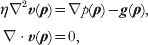
where v(ρ) and p(ρ) are the velocity and pressure of the fluid at the point ρ=(x, y, z) in space, η is the viscosity and g(ρ) is any additional external force (per unit volume) applied to the fluid. The second equation expresses the incompressibility of the fluid and we have assumed a Newtonian stress tensor (Happel & Brenner, Reference Happel and Brenner1983; Kim & Karrila, Reference Kim and Karrila1991)

in writing the first equation. (The symbols ∂i(j) indicate differentiation with respect to the three Cartesian coordinates. That is, ∂i≡∂/ρi, where ρi=x, y or z. This shorthand notation for partial differentiation will be used throughout this review.) Both assumptions (incompressibility and simple Newtonian liquid) are expected to be exceedingly good for the water surrounding the membrane and are commonly adopted approximations used for flow within the membrane itself. We do note that real membranes are compressible and visco-elastic and a more refined treatment may be required for the study of certain problems in the future (see section 5).
In the case of a homogeneous hydrodynamic environment of infinite extent, it is well known that the Stokes equations may be solved to yield the Green's function for velocity driven by point forces (the Oseen tensor) (Doi & Edwards, Reference Doi and Edwards1986). A convenient way to derive this result is via Fourier transformation (Doi & Edwards, Reference Doi and Edwards1986; Kim & Karrila, Reference Kim and Karrila1991). Defining the Fourier transform pair for a generic function f(ρ) as
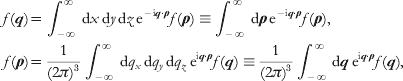
equation (1) is equivalent to


Note that we have adopted the convention of using the same symbol to represent both the real-space function and its Fourier transform – the distinction between the two is implied by the argument. This notation will be convenient for our purposes and is adopted henceforth.
The transformed pressure may be determined by multiplying (i.e. dot product) equation (4) by q and discarding the resulting viscosity term by virtue of the incompressibility condition. This yields p(q)=−iq⋅g(q)/q 2, which may then be inserted into equation (4) to give

The hats indicate vectors of unit length, I is the identity tensor and H(q) is the Fourier transform of the Oseen tensor.
Inverting equation (6) back to real space results in
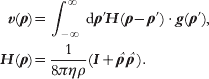
The tensor H(ρ) is the Oseen tensor, specifying the real space velocity response of an infinite fluid to applied forces. The decay of the Oseen tensor with inverse separation between the applied force and induced velocity as well as the particular tensorial character of H are unique to the infinite homogeneous environment that we have assumed. The broader physical content of the Oseen tensor, namely that applied forces instantaneously establish a velocity field everywhere within the fluid and that this field may be expressed as a linear superposition of all applied forces, is a consequence of the creeping flow hydrodynamic limit. The problem of calculating appropriate Green's functions for other hydrodynamic geometries will generally be more difficult than the calculation outlined above. In the remainder of this section, we outline the calculation of some Green's functions relevant to membrane dynamics, which will be referred to later in this review.
2.1 Green's function for in-plane flow within a flat membrane
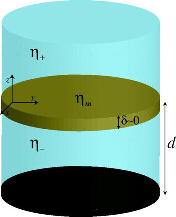
SD (Saffman, Reference Saffman1976; Saffman & Delbrück, Reference Saffman and Delbrück1975) introduced the standard membrane hydrodynamics model for flow parallel to membrane plane. They considered a lipid membrane to be ‘an infinite plane sheet of viscous fluid (lipid) separating infinite regions of less viscous liquid (water)’ (Saffman & Delbrück, Reference Saffman and Delbrück1975). Both the membrane and the bulk fluid surrounding the sheet are treated within the incompressible creeping flow limit, assuming no-slip boundary conditions at the membrane/water interfaces. Although SD was primarily concerned with the diffusion of proteins within the bilayer (translational and rotational), the model itself has far wider applicability. See Fig. 1 for an explanation of the SD geometry.
Our model for flow within the membrane includes a flat membrane surface with vanishing thickness (δ=0) and surface viscosity ηm, with bulk fluids of viscosities η+ and η− lying on either side. The bulk fluids are often assumed to extend infinitely far away from the surface, but in some instances we assume the presence of an impermeable wall a distance d below the membrane. Both the bulk fluids and the membrane are assumed to behave as incompressible Newtonian fluids and are treated within the creeping flow limit. A no-slip boundary condition is assumed between the membrane and surrounding fluids. The membrane is assumed to lie in the x, y-plane. (The traditional SD geometry additionally assumes η+=η−=η and d=∞.)

Hughes, Palitorpe and White (HPW) (Hughes et al. Reference Hughes, Pailthorpe and White1981) extended the original SD analysis to include larger diffusing bodies (e.g. lipid domains). The underlying hydrodynamic model of HPW is identical to that of SD; however, HPW succeeded in relaxing a key approximation in the actual SD calculation of the diffusion coefficient, enabling predictions for bodies of arbitrary size. The SD membrane model has also been applied to understand the dynamics of shape fluctuations in nearly circular lipid domains (Alexander et al. Reference Alexander, Bernoff, Mann, Mann, Wintersmith and Zou2007; Camley et al. Reference Camley, Esposito, Baumgart and Brown2010; Stone & McConnell, Reference Stone and McConnell1995). Perhaps the most practical mathematical formulation of the SD hydrodynamic model is given by the in-plane Green's function for membrane flow, the analog to the Oseen tensor appropriate for membrane geometries and flow within the membrane plane. Introduced by Lubensky and Goldstein (Lubensky & Goldstein, Reference Lubensky and Goldstein1996), the membrane Green's function has been used to reproduce the prior theoretical results for diffusion and domain shape fluctuations (Camley et al. Reference Camley, Esposito, Baumgart and Brown2010; Lubensky & Goldstein, Reference Lubensky and Goldstein1996; Oppenheimer & Diamant, Reference Oppenheimer and Diamant2009) and represents a formulation of the SD hydrodynamic problem that is especially appealing for numerical simulations.
In order to derive the membrane Green's function, we begin with the Stokes equations for flow within the membrane
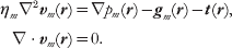
These equations are similar to those of the bulk 3D fluid, but represent 2D flow (we assume that the membrane lies in the x, y-plane as in Fig. 1 so that r=(x, y) and the vector derivatives correspondingly act only in the x and y directions). ηm is thus a surface viscosity with dimensions of viscosity⋅length and the ‘pressure’ p m is actually a force per unit length. The vector quantities gm and t are forces per unit area with gm taken to represent the effect of externally applied forcing and t representing the traction on the membrane surface imposed by the surrounding solvent.
The primary difficulty associated with equation (8) is the traction term. In the absence of this contribution, one could immediately proceed via Fourier transformation as in 3D. In fact, a 2D Fourier basis is still convenient, but we must first solve for influence of the bulk fluid on the velocity field within the membrane. We take advantage of the observation by Stone and McConnell (Stone & McConnell, Reference Stone and McConnell1995) that the bulk pressure (p) is constant in the subfluid above and below a plane with 2D incompressibility, for in-plane forces confined within the membrane sheet. This considerably simplifies the 3D Stokes equations for the subfluids (equation (1)), resulting in loss of the ∇p term and rendering the equation equivalent to the Laplace equation when no body forces are present in the bulk. If we Fourier transform only with respect to the (x, y) variables, we find (we assume η+=η−=η as in the traditional SD picture)

where we have introduced the wavevector k=(k x, k y), which is distinct from q in that it only involves the 2D Fourier variables. Note that our adopted notation convention specifies that, for example, v+(k, z) is the partially Fourier transformed velocity, with transformation only over x and y. Through the no-slip boundary condition, the velocity of the membrane is equal to the bulk fluid velocity immediately above and below the bilayer vm(r)=v+(r, z=0)=v−(r, z=0). Equation (9) is immediately solved to give v±(k, z)=vm±(k, 0)e∓kz and the traction imparted by the subfluids to the membrane follows from the Newtonian stress tensor for the subfluids (equation (2))

We may thus write the transformed version of equation (8)


Proceeding in an analogous fashion to the 3D case, we arrive at

where we have introduced the SD length scale L SD=ηm/2η.
The real-space version of the tensor T involves a complicated collection of special functions and is not particularly illuminating (Oppenheimer & Diamant, Reference Oppenheimer and Diamant2009). However, by looking at equation (13), it is easy to grasp the essential physical content of Green's function. For sufficiently large wavelengths (i.e. k<<L SD−1), the expression looks like ~k −1, which is the 2D transform of 1/r. For large-scale flows, the membrane behaves similar to what would be expected in 3D (see equation (7)); it is the flow in the surrounding fluid that is dominating the hydrodynamics. In the opposite limit (k>>L SD−1) corresponding to short wavelengths, the expression approaches a k −2 behavior, which is characteristic of the logarithmic divergences seen in purely 2D fluids; it is the flow within the membrane itself that dominates the small wavelength behavior of the system.
It is worth emphasizing that the above-sheet and below-sheet tractions contribute to the total traction in additive fashion, so that the ηmL SD−1k=2ηk term appearing in the denominator of T(k) derives from the summed contribution of ηk from the solvent above the membrane sheet and ηk from the solvent below the sheet. A membrane separating two semi-infinite homogeneous fluids with disparate viscosities would thus replace 2ηk with (η++η−)k. Lubensky & Goldstein (Reference Lubensky and Goldstein1996) have also calculated tractions for the case that the subfluids are confined within regions of finite depth d ± (no-slip boundary conditions are assumed on the wall confining the fluid)

It thus becomes possible to specify hydrodynamic kernels associated with in-plane flow on membranes residing in varied fluid environments. For example, a crude model for motion on the surface of a biological cell might call for aqueous solution with the viscosity of water ηw above the membrane (extending to infinity) and higher viscosity ηc cytoplasm confined within a slab of thickness d (the ‘size’ of the cell) beneath the membrane. Such an environment results in

More traditionally, this sort of approach (Fischer, Reference Fischer2004; Oppenheimer & Diamant, Reference Oppenheimer and Diamant2010; Lubensky & Goldstein, Reference Lubensky and Goldstein1996; Stone & Ajdari, Reference Stone and Ajdari1998) allows for the analysis of model membrane systems in common experimental geometries, which often involve subfluids of finite depth.
2.2 Green's function for small amplitude out-of-plane membrane deformations
A completely different aspect of membrane dynamics involves the out-of-plane motion of the membrane itself. For arbitrary membrane geometries, these motions will couple to in-plane flow (Henle & Levine, Reference Henle and Levine2010; Yoon & Deutsch, Reference Yoon and Deutsch1997), resulting in a problem of greater complexity (and generality) than considered in this review. However, if we consider small fluctuations in shape about a flat reference configuration, the out-of-plane dynamics decouple from in-plane flow and a simplified description is possible (Brochard & Lennon, Reference Brochard and Lennon1975; Levine & MacKintosh, Reference Levine and MacKintosh2002).
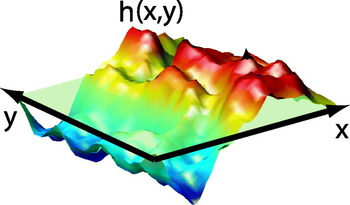
The shape of a thin, nearly flat surface (membrane) is completely determined by specifying the local height h(x, y)=h(r) at which the surface may be found above the reference x, y-plane (see Fig. 2). (The ‘nearly flat’ condition is assumed to guarantee no overhangs of the membrane in the sense that h(r) is single valued. A perfectly flat membrane is specified by the condition h(r)=0.) We invoke the simplifying approximation of substituting the hydrodynamic interaction for the h(r)=0 geometry regardless of the exact membrane shape, ignoring surface corrugation for the purposes of determining hydrodynamic coupling. This approximation is most convincingly justified when the h(r)=0 shape represents the free energy minimum for the sheet; deviations from the flat state then result in restoring forces that contain only linear and higher-order contributions in h (i.e. there is no zeroth-order contribution to the force). A linearized equation of motion for h(r)=0 will therefore necessarily involve only the zeroth-order (h(r)=0) hydrodynamic coupling, since any corrections stemming from non-flat geometry would lead to quadratic and higher-order terms in the dynamics. More generally, when non-linear equations of motion are considered and/or the minimum energy configuration is not perfectly flat (as in some of the cases considered later in this review), the use of the h(r)=0 hydrodynamic kernel should be viewed as a convenient, but ultimately uncontrolled, simplifying approximation.
A nearly flat surface may be described by the local deviation of the surface from a planar fiducial state (pale green). As long as there are no overhangs, the height function h(x, y) is single valued for all points in the xy-plane and provides a complete description of surface shape. The surface is said to be described in the ‘Monge gauge’ or ‘height representation’.

We consider the Stokes equations for the upper and lower subfluids surrounding the membrane in our fiducial h(r)=0 geometry. In contrast to the preceding section, the study of membrane shape dynamics explicitly considers the velocity of the membrane in the direction normal to the surface (i.e. ∂th(r)≡ (r)), and the corresponding flows in the z-direction associated with the bulk fluids v z±(ρ). With motions directed normal to the membrane surface, in-plane membrane incompressibility no longer guarantees a constant pressure within the bulk. However, in the absence of forcing (g=0) equation (1) still considerably simplifies. The analog to equation (9), employing the same partial Fourier transformation in (x, y), but including the effect of non-constant pressure driven by membrane motion in z is

Here, we have restricted focus to the z-component of fluid motion, which provides the necessary information to determine (r). This equation is simply the biharmonic equation ∇4v z±=0, which follows from the condition ∇2p=0 in the absence of forcing and taking the Laplacian of the Stokes equation. This equation has the general solution

where c i's are determined by boundary conditions.
We will use the notation Λ(r) to represent Green's function for z-directed velocity response to z-directed forces at the membrane surface. That is, we write


where F(r) is the force per unit area acting on the membrane, directed normal to the surface. The first equality in each case follows from the no-slip condition at the membrane surface. Force balance between hydrodynamic stress and force on the bilayer implies

and the hydrodynamic kernel is therefore given by

A given set of boundary conditions leads to explicit expressions for v z±(k, z), p(k, z) and, via equation (2), ∏zz±(k). Λ(k) then follows immediately from equation (20).
As a concrete example of the preceding analysis, we calculate Λ(k) for the case of a membrane embedded in an infinite bulk fluid with viscosity η. Since the velocity of the fluid must decay to zero far from the membrane, this immediately confines our search for solutions to the appropriately decaying terms in each half-plane found in equation (17). Furthermore, the symmetry of the environment surrounding the membrane immediately suggests that v+(k, z)=v−(k, −z) and the no-slip condition at the membrane surface (equation (18)) dictates v z+(k, z=0)=v z−(k, z=0)=(k). Taken together, these boundary conditions and a minimal amount of algebra immediately imply



and finally, on substitution into equation (20)

The ‘inf’ superscript simply indicates that this hydrodynamic kernel corresponds to the case of an infinite homogeneous fluid surrounding the membrane. It is worth mentioning that nowhere in this example did we rely on the in-plane incompressibility of the membrane to derive Λinf(k), only the behavior of the surrounding bulk fluid was necessary to derive the result. Knowing this, a much faster derivation is possible, as shown by Granek (Reference Granek1997) . Since the out-of-plane membrane hydrodynamic response was found to be governed solely by the fluid, it should be equivalent to the zz component of the Oseen tensor for separation vectors ρ lying within the xy-plane. In other words, Λinf(k)=H zz(k, z=0). Since H zz(k, z=0) involves only a 2D Fourier transform, we cannot immediately apply equation (6), but must calculate

which evaluates to give equation (24).
As in the preceding section, equation (24) may be generalized to incorporate viscosity contrast between the fluids on either side of the membrane and/or the presence of an impermeable wall near the membrane (Gov et al. Reference Gov, Zilman and Safran2004; Lin & Brown, Reference Lin and Brown2006; Seifert, Reference Seifert1994). In these cases, the algebra involved in satisfying boundary conditions is more tedious and, in the case of the wall, the specific model of the membrane (i.e. in-plane incompressibility) does affect the hydrodynamic kernel. For completeness, we quote a general result here that includes the presence of an impermeable no-slip wall at a distance d beneath the membrane (i.e. v−(k, z=−d)=0) and viscosities of fluid η+ and η− above and below the membrane respectively. The fluid above the membrane is assumed to extend to infinity:

where we have introduced  ,
 and
 to keep the expression as concise as possible. Note that in the limit d→∞, the general result reduces to
 , which is just the result derived earlier in the case of an infinite medium, but incorporating the mean viscosity of the two bounding fluids. The effect of the wall is to slow down the relaxation of the membrane, which will be clearer in the following sections.
2.3 Some comments on practical application of Green's functions
The following sections of this review will focus on the calculation and simulation of membrane dynamics, making use of the hydrodynamic interactions derived above. The observant reader will already have noticed that we have focused the bulk of our attention on deriving the 2D Fourier-transformed Green's functions: T(k) (equations (13) and (15)) and Λ(k) (equations (24) and (26)) and have not been overly concerned with inverting these expressions back to real space. Partially, this is due to convenience; the mathematical expressions are far simpler in k-space than real space. However, a more compelling argument for thinking in terms of the transformed interactions is based on certain unavoidable computational realities. The equations of motion discussed in the following sections will always include contributions such as equations (7) and (18), with some velocity calculated as the convolution between a force field and the relevant Green's function for velocity response. The natural way to evolve these equations is via Fourier transformation, where the convolution is handled as a simple product. The computational expense of fast Fourier Transformation (FFT) (Press et al. Reference Press, Teukolsky, Vetterling and Flannery1994) is far lower than that required to evaluate the convolution directly for all r points in real space. We will also see that the Fourier description provides a natural way to deal with some of the energetics/forces involved in the membrane models themselves.
One small caveat to the above argument is that the Fourier transforms introduced above (equation (3) and its 2D generalization) assume an infinitely large system in the x, y-plane. For our numerics, we will always assume periodic boundary conditions on the membrane so that our wavevectors k are confined to discrete values obeying the condition  with integer valued n and m. We will write the Fourier pair for an arbitrary function f(r) periodic over an
 × box as
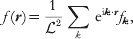

The way such periodic functions will show up in practice is typified by equation (18). Since the membrane is assumed to be periodic, both the membrane height field h(r) and the forces acting on it, F(r) must be periodic. The Green's function for the hydrodynamic response Λ(r) is not periodic and equation (18) reflects contributions to the velocity stemming from all periodic images of the force through space. We calculate  by transforming equation (18) as defined above
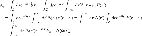
with the understanding that k satisfies the periodicity condition introduced above. It is important to recognize that although this expression has the appearance of the usual convolution rule, the Green's function has been Fourier transformed, whereas the quantity relevant to the current configuration of the membrane is a Fourier series expansion coefficient. This has both physical significance (i.e. the Green's function is not periodic, whereas the membrane is) as well as purely practical implications regarding inversion of the terms back to real space (via equations (3) and (27)) and how to calculate the various pieces. For this reason, we will retain the notation where subscripted Fourier variables represent the elements of a Fourier series, whereas a traditional function notation (e.g. f(k)) will imply Fourier transformation.
As a final comment, we note that the Fourier series defined in equation (27) will always be truncated at some maximal wavevector. In practice, for simulations, we must always consider a short-wavelength cutoff by imposing the restriction −N/2<<m, n⩽N/2, where N is some integer. This choice sets the number of dynamical variables evolved in the simulations at N 2 and defines a minimum length scale ℓ (N=/ℓ) captured in the modeling. Physically, one might expect ℓ to be comparable to the dimensions of a single lipid as the elastic approximation is certain to break down for wavelengths below molecular resolution. In practice, we often take ℓ to be somewhat larger, reflecting ambiguity in experimental results at short wavelengths and/or allowing for less taxing computations. We typically find that our numerical results are not sensitive to the exact cutoff imposed, so long as the observables being studied correspond to sufficiently long wavelengths with the cutoff falling well below any mesoscopic length scales important to the problem at hand (e.g. the interface with between phases). All our simulations ultimately come down to evolving these N 2 variables using numerical schemes that rely heavily on the FFT operation. In some sense, all the reported simulations may be viewed as implementations of the traditional ‘Brownian dynamics with hydrodynamic interactions’ introduced by Ermak & McCammon (Reference Ermak and McCammon1978)
; we are simply evolving overdamped stochastic equations of motion that include hydrodynamic interactions at the creeping flow level.
3. Simulations of phase separation and lipid domain fluctuations in model membrane systems
Ternary mixtures of saturated and unsaturated lipids and cholesterol have become a standard experimental model to study the dynamics of inhomogeneous membranes under controlled laboratory conditions (Berkowitz, Reference Berkowitz2009; Veatch & Keller, Reference Veatch and Keller2005). These dynamics include: diffusion of lipid domains (Cicuta et al. Reference Cicuta, Keller and Veatch2007), ‘flickering’ fluctuations of domain boundaries (Esposito et al. Reference Esposito, Tian, Melamed, Johnson, Tee and Baumgart2007) and phase separation kinetics (Veatch & Keller, Reference Veatch and Keller2003). Analytical calculations for domain diffusion and flickering in certain regimes have helped to illuminate the relevant physics (Hughes et al. Reference Hughes, Pailthorpe and White1981; Stone & McConnell, Reference Stone and McConnell1995), which crucially depends on the hydrodynamic environment of a viscous fluid membrane suspended within bulk solvent (Lubensky & Goldstein, Reference Lubensky and Goldstein1996; Saffman & Delbrück, Reference Saffman and Delbrück1975). Although most experiments to date have concentrated on vesicle morphologies, the analysis presented here presumes a flat membrane surface for mathematical convenience. Comparisons between experiment and theory/simulation under these circumstances should be confined to length scales that are much smaller than both the vesicle size (experiment) and the dimensions of the periodic box (simulation).
3.1 Specification of the physical model
Our focus is on experimentally observable dynamics, not first-principles prediction of detailed thermodynamic properties. Accordingly, we adopt a standard Landau–Ginzburg-free energy functional for binary mixtures (Chaikin & Lubensky, Reference Chaikin and Lubensky2000; Safran, Reference Safran1994):

where ∊, u, γ>0. Equation (30) may be interpreted as a phenomenological description of the observed two-phase coexistence in ternary lipid/cholesterol systems. However, to facilitate comparison with experiment, we assume tight stoichiometric complexation between cholesterol and the saturated lipid (McConnell, Reference McConnell2005) and identify φ(r)≡χ(r)unsaturated−χ(r)complex as the local difference in mole fraction (χ) between lipid species. Although limited to mixtures with a 1:1 stoichiometry between saturated lipids and cholesterol, this picture has the advantage of simplicity: only a single composition field is required and the three parameters appearing in F are readily related to measurable experimental properties (Safran, Reference Safran1994): the line tension between phases,  , interface width
 and equilibrium phase compositions
 .
From the standpoint of system energetics, similar phase-field approaches to the above have been adopted previously (Fan et al. Reference Fan, Sammalkorpi and Haataja2010; Funkhouser et al. Reference Funkhouser, Solis and Thornton2007; Reigada et al. Reference Reigada, Buceta, Gomez, Sagues and Lindenberg2008). Our primary theoretical contribution has been in the development of a phase-field model that properly accounts for the unique quasi-2D membrane hydrodynamic environment and thermal fluctuations. We require the dynamics of φ to conserve lipid concentrations, hydrodynamically couple points on the membrane and include thermal fluctuations. Model H dynamics represents the generic long-wavelength low-frequency picture to incorporate these requirements (Chaikin & Lubensky, Reference Chaikin and Lubensky2000). In the creeping-flow limit, model H reduces to (Bray, Reference Bray1994; Koga & Kawasaki, Reference Koga and Kawasaki1991)


Although typically applied to pure 3D or 2D geometries, we use equation (31) for the quasi-2D fluid membrane geometry introduced in section 2.1. In this case, v=(v x, v y) is the in-plane membrane velocity field, M is a transport coefficient related to the collective diffusion coefficient for lipids within the bilayer (D φ) via M=D φ/2r (Chaikin & Lubensky, Reference Chaikin and Lubensky2000; McWhirter et al. Reference McWhirter, Ayton and Voth2004) and T ij(r) is the Green's function for in-plane velocity response of the membrane to a point force. In what follows, we assume an infinitely large homogeneous embedding fluid surrounding the membrane and use equation (13) for T ij(r). The other hydrodynamic environments discussed in section 2.1 are easily implemented as well, with only trivial modifications to the below considerations. The Gaussian white thermal noise terms, θ(r, t) and ζj(r′, t), are distributed with variances set by the fluctuation–dissipation theorem (Van Kampen, Reference Van Kampen2007) and must be handled within the Stratanovich interpretation (Gardiner, Reference Gardiner1985; Van Kampen, Reference Van Kampen2007). In equation (31) and henceforth, the Einstein summation convention is assumed. Equation (31) has been written over two lines to emphasize the fact that it represents a simple dissipative dynamics for the conserved field φ as viewed from the frame of a particle moving with the fluid. However, the creeping flow limit dictates that the velocity field v is completely specified by the instantaneous configuration of the composition field φ (and the random force ζ). The scalar field φ is the only independent field in the dynamics; v is defined purely as a notational and pedagogical convenience.
Recall from section 2.1 that T(r) displays a crossover in physical behavior from 2D response to 3D-like response, with L sd=ηm/2η governing the approximate crossover point. In typical model membrane systems, ηm ranges from (0·1−10)×10−6 surface poise (poise-cm or grams/s) (Cicuta et al. Reference Cicuta, Keller and Veatch2007; Dimova et al. Reference Dimova, Dietrich, Hadjiisky, Danov and Pouligny1999; Petrov & Schwille, Reference Petrov and Schwille2009), corresponding to L sd~0·1−10 μm. Fluorescence microscopy experiments probe wavelengths comparable to L sd and it is critical to use the full expression in comparison with these experiments.
Koga & Kawasaki (Reference Koga and Kawasaki1991)
suggested the use of FFT as an efficient way to numerically evolve zero-temperature overdamped model H dynamics. We extend their approach with modifications for the quasi-2D hydrodynamic environment and stochastic thermal forces. An × periodic geometry is assumed; the dynamics of the Fourier modes φk follow from equation (31):
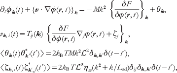
where {f(r)}k is the Fourier transform of f(r). These equations are solved numerically by truncating to N Fourier modes k=(m, n)2π/ with −N/2<<m, n⩽N/2 (corresponding to a real-space discretization size ℓ=/N). {…}k terms are evaluated in a hybrid real-space/Fourier-space fashion, handling real-space derivatives and convolutions in k-space, local real-space operations in r-space and moving between the two representations via the FFT (Camley & Brown, Reference Camley and Brown2010). The time evolution is accomplished via a semi-implicit Stratonovich integrator (Kloeden & Platen, Reference Kloeden and Platen1999; Zhu et al. Reference Zhu, Chen, Shen and Tikare1999). Details of the numerical implementation may be found in the supplementary material to reference (Camley & Brown, Reference Camley and Brown2010).
We emphasize that the equations governing our simulations are non-linear in φ due to both the v⋅∇φ term within equation (31) as well as the quartic nature of our free energy. Although certain consequences of these dynamics may be predicted analytically for specific limiting regimes (see the next two sections), general solution of the equations requires simulations to be performed. These simulations are unique within the continuum-membrane literature due to the incorporation of both the proper quasi-2D membrane hydrodynamic geometry and thermal fluctuations. Although dissipative particle dynamics (DPD) and related particle-based simulation schemes have been used to study composition dynamics in membrane systems previously (Laradji & Kumar, Reference Laradji and Kumar2005; McWhirter et al. Reference McWhirter, Ayton and Voth2004; Ramachandran et al. Reference Ramachandran, Komura and Gompper2010), the approach discussed above has distinct advantages relative to such techniques: experimental length and time scales may be directly simulated, the model is completely specified via direct input of a handful of physically meaningful parameters {σ, ξ, φ0, η, ηm, D φ} and the hydrodynamic environment is easily tuned to reflect an infinite bulk surrounding medium or any one of the other cases discussed in section 2.1. The implicit treatment of the hydrodynamics is especially convenient, since it is not necessary to expend the bulk of computational effort tracking solvent. Of course, DPD methods are inherently more versatile than the phase-field approach discussed here; the same model may be used to study planar, vesicle and other bilayer geometries and it is a simple matter to extend the models to multiple lipid species and other complications. It is important to recognize that both approaches (DPD and continuum models) are complementary in the study of membrane composition dynamics.
3.2 Diffusion of lipid domains
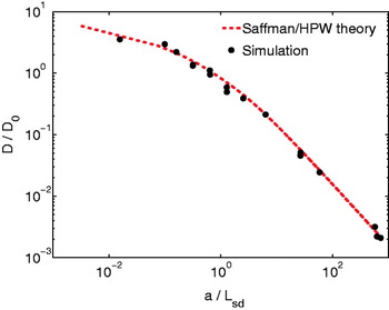
The translational diffusion of circular lipid domains presents an ideal test to confirm the validity of the simulation method. Analytical theory based on the same quasi-2D hydrodynamics outlined above predicts (Hughes et al. Reference Hughes, Pailthorpe and White1981; Saffman & Delbrück, Reference Saffman and Delbrück1975) D a=(k BT/4πηm) (a/L sd) for the diffusion coefficient of a circular body of radius a within a SD membrane. The function represents the solution to an integral equation and is not available in closed form (Hughes et al. Reference Hughes, Pailthorpe and White1981), but it is well approximated by a closed-form empirical fit described in Petrov & Schwille, (Reference Petrov and Schwille2009)
. Experiments tracking the position of lipid domains have confirmed these theoretical results in the context of real lipid-bilayer systems (Cicuta et al. Reference Cicuta, Keller and Veatch2007; Petrov & Schwille, Reference Petrov and Schwille2009; Sakuma et al. Reference Sakuma, Imai, Urakami, Nagao, Komura and Kawakatsu2010) and we expect similar agreement between theory and our simulations. Choosing initial conditions to reflect a single circular domain and thermodynamic parameters that guarantee the domain remains nearly circular (high σ, low T), we track the simulated domain's position over time and infer D a via its mean square displacement. The results collapse onto (a/L sd) (all of a, ηm and η were independently varied) over a wide range of a/L sd ratios, completely spanning the crossover between SD diffusion D a~ln(L sd/a) in the limit of small domains and Stokes–Einstein-like diffusion D a~1/a in the limit of large domains (Fig. 3), which provides a compelling verification of the methodology over a range of length/time scales.
Translational diffusion coefficients obtained by tracking simulated domain motion, compared with Saffman–Delbrück–Hughes–Pailthorpe–White theory (using the interpolation of Petrov & Schwille (Reference Petrov and Schwille2009) ). D 0=k BT/4πηm. Error bars are of the order of marker size. Line tensions and temperatures were chosen to ensure domains remained circular over the course of the simulations; box sizes range from 10 μm to 40 μm (N=256–1024), chosen to eliminate effectsfrom periodic boundary conditions.

3.3 Shape fluctuations of lipid domains
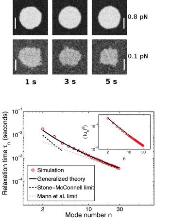
In experimental membrane systems, line tensions are seldom high enough to fully suppress shape fluctuations of lipid domains. Although these fluctuations have minimal impact on translational diffusion, the fluctuations themselves may be analyzed (Esposito et al. Reference Esposito, Tian, Melamed, Johnson, Tee and Baumgart2007) and provide a further test of our simulation methods. Evolving an initially circular domain by equations (32), we found, in agreement with Frolov et al. (Reference Frolov, Chizmadzhev, Cohen and Zimmberg2006), that domains with small line tensions ~0·1−0·2 pN are not thermodynamically stable at temperatures ~20°C and area fractions ~0·03−0·1; the domain radii shrink over time in favor of a more homogeneous distribution through the simulation box (Fig. 4).
Top: simulated evolution of a flickering domain with initial radius R=2·0 μm, ηm=1×10⁻⁶ surface poise, σ=0·8, 0·1 pN and ξ=40 nm. The collective diffusion coefficient  cm2/s. N=512, and the time step Δt is 5 μs. T=21°C, η=0·01 Poise. These are typical values for ternary domains near 20°C, with a viscosity in the middle of the commonly accepted range (see text). The σ=0·1 pN domain shrinks, whereas the σ=0·8 pN domain is stable. The box size for the simulation is 20 μm×20 μm (scale bar: 2 μm). Only the region immediately surrounding the domain is displayed. Bottom: relaxation times for mode n for σ=0·8 pN (see text). The theoretical predictions are summarized in equation (33). Inset: thermal variance in amplitude for mode n. The theoretical prediction (black) is the equipartition result described in the text. There is no fitting involved foreither the main figure or inset. Theoretical predictions follow immediately from the parameters input to the model and demonstrate the robustness of the simulation scheme.

At higher line tensions, domains under similar thermodynamic conditions are stable and we have simulated the dynamic fluctuations of these systems (Fig. 4) We use the image analysis techniques of Esposito et al. (Reference Esposito, Tian, Melamed, Johnson, Tee and Baumgart2007), tracing the boundary of the domain, and expanding it into quasi-circular modes,  . For small deviations u n, the domain shape is expected to behave in accord with an effective Hamiltonian governed by the line tension at the domain boundary
 (L is the domain perimeter). If this effective quadratic Hamiltonian is valid, 〈|u n|〉2=2k BT/σπR 0(n 2−1) is expected via equipartition. Experimentally, this relation is used to determine line tensions (Esposito et al. Reference Esposito, Tian, Melamed, Johnson, Tee and Baumgart2007). We observe that our numerical experiments yield the equipartition result with the expected
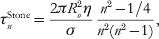
 (Fig. 4, inset). The linear dynamics of these modes depend on the line tension as well as the viscosities of both the membrane and the surrounding fluid; 〈u n(t)u −n(0)〉=〈|u n|2〉et/τn. Stone and McConnell found these relaxation times neglecting the membrane viscosity (valid for length scales R/n>>L sd) and Mann et al. calculated them neglecting the bulk fluid (valid for R/n<<L sd) (Mann et al. Reference Mann, Hénon, Langevin, Meunier and Léger1995; Stone & McConnell, Reference Stone and McConnell1995). In our simulations, we see exponential relaxation over all modes u n(t) with τn plotted in Fig. 4. We note that for large n modes, the Mann theory is appropriate, as expected, but there are deviations from the Stone–McConnell result even at low n since L sd=0·5 μm is comparable to the size of the domain. The simulations are in excellent agreement with a recent generalization to the Stone–McConnell theory (Camley et al. Reference Camley, Esposito, Baumgart and Brown2010) that includes the effects of both ηm and η, providing yet another validation of the simulation model. For reference, we include the three theoretical expressions here:


where J n(x) is a Bessel function of the first kind.
3.4 Phase separation in ternary model systems
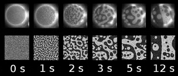
The modeling described in this section displays its true potential when applied to problems that are not readily explained with analytical theory. Using identical methodology to the diffusion and fluctuation studies, but employing a homogeneous initial condition, allows the study of phase separation kinetics in ternary lipid/cholesterol model systems. Our simulations are motivated by the experiments of Veatch and Keller (Veatch and Keller, Reference Veatch and Keller2003) on roughly 1:1:1 mixtures of DOPC/DPPC/Chol. Taking care to choose parameters consistent with the experimental system, we find good agreement between simulation and experiment (Fig. 5). The model uses eight physical parameters (T, σ, ξ, φ0, D φ, η, ηm, ). The temperature T=21°C, box size =30 μm and viscosity of water η=1 cP follow immediately from the experimental conditions. The remaining five parameters specify details of the specific bilayer system under study. Although precise measurements of all these parameters are not available, the numbers are known approximately, either for the specific DOPC/DPPC/Chol system under study or by analogy to other model systems expected to show similar behavior. φ0=0·4 may be determined from the DOPC/DPPC/Chol phase diagram (Cicuta et al. Reference Cicuta, Keller and Veatch2007). The line tension σ=0·1 pN is based on flicker spectroscopy measurements of DOPC/DPPC/Chol mixtures (Esposito et al. Reference Esposito, Tian, Melamed, Johnson, Tee and Baumgart2007), which also sets the correlation length ξ=40 nm via the relation σξ=k BT (Baxter, Reference Baxter1982), a theoretical result for the Ising model, supported by experiments in ternary lipid systems (Honerkamp-Smith et al. Reference Honerkamp-Smith2008). The transport coefficients ηm=5×10⁻⁶ surface Poise and D φ=7×10⁻¹⁰ cm2/s are difficult to precisely measure and are not known experimentally for the exact system studied here. The values chosen are consistent with measurements in related lipid systems (Korlach et al. Reference Korlach, Schwille, Webb and Feigenson1999; Petrov & Schwille, Reference Petrov and Schwille2009) and the requirement that  (Saffman & Delbrück, Reference Saffman and Delbrück1975).
Comparison of experimental (top) and simulated (bottom) phase separation kinetics for 1:1:1 mixtures of DOPC/DPPC/Chol. Experimental figure adapted from Veatch and Keller (vesicle diameter is 30 μm) (Veatch & Keller, Reference Veatch and Keller2003). See text for physical parameters and =30 μm, N=1024 and Δt=20 μs.

The similarity between experiment and theory in Fig. 5 is striking and demonstrates that complex non-linear bilayer dynamics over micron length scales and second time scales may be directly studied numerically. The displayed results depend on both membrane and solvent viscosity; a naive 2D simulation assumes the wrong dissipation for length scales above L sd(~1 μm) and correspondingly incorrect time scales. More interestingly, dynamics of quasi-2D membrane phase separation are qualitatively different from the pure 2D or 3D cases. We observe dynamical scaling with a continuous morphology, with length scale R(t)~t 1/2 for critical mixtures (1:1:1) when R(t)>>L sd (Camley & Brown,Reference Camley and Brownin press). The R(t)~t 1/2 behavior is predicted by simple scaling arguments (as in Bray, Reference Bray1994) and is qualitatively different from coarsening in 2D or 3D. In 2D, dynamical scaling is not observed (Wagner & Yeomans, Reference Wagner and Yeomans1998) and in 3D, one expects R(t)~t (Bray, Reference Bray1994). A simple model for dynamics incorporating only diffusive transport and neglecting advection (i.e. Cahn–Hilliard dynamics (Bray, Reference Bray1994; Chaikin & Lubensky, Reference Chaikin and Lubensky2000)) would predict R(t)~t 1/3 (Bray, Reference Bray1994; Wagner & Yeomans, Reference Wagner and Yeomans1998; Zhu et al. Reference Zhu, Chen, Shen and Tikare1999).
This section (and the immediately preceding example in particular) demonstrates that poorly considered approximations for the hydrodynamic environment can lead to clear qualitative inconsistencies for certain aspects of membrane dynamics. It seems unlikely that there is any way to compensate or otherwise convincingly repair a simulation run within the wrong hydrodynamic environment. In particular, it seems that particle-based solvent-free models (Brannigan et al. Reference Brannigan, Lin and Brown2006) have no hope of reproducing membrane dynamics. More distressingly, it is potentially very dangerous to run explicitly solvated models (either fully atomic or coarse grained) within narrow (small z dimension) simulation boxes. The bulk hydrodynamic flows accompanying motion within the membrane plane do decay with distance from the membrane (see discussion beneath equation (9)); however, these bulk flows fall off only as fast in the z-direction as the wavelength for the in-plane flow. To be assured that one is running a simulation corresponding to an effectively infinite bulk embedding fluid would require a box somewhat larger in the z dimension than in the x, y – such conservative boundary conditions are seldom, if ever, implemented within particle-based simulations. The implicit treatment of bulk solvent flow is one of the primary appealing facets of the continuum approach described here. It is important to recognize the possible hydrodynamic deficiencies associated with particle-based simulations. Even those approaches that would seem on cursory inspection to account for solvent flow, may not have sufficient solvent present to allow for a direct comparison with experiment or theoretical predictions that presume a large homogenous environment around the membrane.
Our dynamic phase-field model is consistent with experimental (Camley et al. Reference Camley, Esposito, Baumgart and Brown2010; Cicuta et al. Reference Cicuta, Keller and Veatch2007; Petrov & Schwille, Reference Petrov and Schwille2009; Sakuma et al. Reference Sakuma, Imai, Urakami, Nagao, Komura and Kawakatsu2010; Veatch & Keller, Reference Veatch and Keller2003) and theoretical results (Camley et al. Reference Camley, Esposito, Baumgart and Brown2010; Mann et al. Reference Mann, Hénon, Langevin, Meunier and Léger1995; Saffman & Delbrück, Reference Saffman and Delbrück1975; Stone & McConnell, Reference Stone and McConnell1995) for a wide variety of length scales and phenomena. More interestingly, our results suggest that the hydrodynamic environment surrounding the membrane must be carefully considered in any simulation methodology; an incorrect hydrodynamic geometry can lead to spurious results. Simulations of the type described here represent an important step toward the modeling of complex biological membranes over length and time scales relevant to cellular biology. Extensions of this picture to out-of-plane membrane undulations, coupling to cytoskeleton and integral membrane proteins are underway (see the following sections) and should prove invaluable for the study of a large class of problems in membrane biology and biophysics.
4. Simulations of membrane shape fluctuations
The previous section assumed a completely flat membrane surface. We now consider the possibility of membrane shape fluctuations within an elastic continuum approach. The elastic description of cell membranes is now a traditional subject in the sense that treatments may be found in review articles and books (Boal, Reference Boal2002; Evans & Skalak, Reference Evans and Skalak1980; Lipowsky, Reference Lipowsky1991; Nelson et al. Reference Nelson, Piran and Weinberg2004; Safran, Reference Safran1994). Historically, the elastic level of description has been useful primarily as an analytical tool, by providing tractable expressions to compare with experiment or to understand the generic long-wavelength physics of the simplest model systems. Among the many biophysical problems studied with such an approach are the shape (Canham, Reference Canham1970; Deuling & Helfrich, Reference Deuling and Helfrich1976; Helfrich, Reference Helfrich1973; Lim et al. Reference Lim, Wortis and Mukhopadhyay2002; Mukhopadhyay et al. Reference Mukhopadhyay, Lim and Wortis2002) and fluctuation dynamics (Brochard & Lennon, Reference Brochard and Lennon1975; Fournier et al. Reference Fournier, Lacoste and Raphael2004; Gov et al. Reference Gov, Zilman and Safran2003) of human red blood cells (RBC), the shape transformations of vesicles (Lipowsky, Reference Lipowsky1991; Miao et al. Reference Miao, Fourcade, Rao, Wortis and Zia1991, Reference Miao, Seifert, Wortis and Döbereiner1994; Seifert & Lipowsky, Reference Seifert, Lipowsky, Lipowsky and Sackmann1995; Seifert et al. Reference Seifert, Berndl and Lipowsky1991), the influence of membrane elasticity on integral membrane protein stability (Fattal & Ben-Shaul, Reference Fattal and Ben-Shaul1993; Helfrich & Jakobsson, Reference Helfrich and Jakobsson1990; Huang, Reference Huang1986; Nielsen et al. Reference Nielsen, Goulian and Andersen1998; Partenski & Jordan, Reference Partenskii and Jordan2002), the ‘lipid mediated’ (Marčelja, Reference Marčelja1976) interactions between multiple membrane proteins (Goulian et al. Reference Goulian, Bruinsma and Pincus1993; Kim et al. Reference Kim, Neu and Oster1998), the dynamics of ‘active’ vesicles under the influence of energy-consuming proteins (Gov, Reference Gov2004; Lin et al. Reference Lin and Brown2006; Prost & Bruinsma, Reference Prost and Bruinsma1996; Prost et al. Reference Prost, Manneville and Bruinsma1998), the entropically driven inter-membrane repulsions in lamellar membrane stacks (Helfrich, Reference Helfrich1978; Lipowsky, Reference Lipowsky1991) and the softening of elastic moduli with the size of the membrane system (Helfrich, Reference Helfrich1985; Peliti & Leibler, Reference Peliti and Leibler1985). Although certainly not inclusive of all studies in the literature, the above list hopefully conveys a sense of the diversity of biophysical problems well suited to the elastic level of membrane modeling with analytical calculation.
Surprisingly, relatively little work has been done extending elastic membrane models into the simulation regime. While numerical minimization of elastic membranes in various geometries and under the influence of external stresses is quite common (Discher et al. Reference Discher, Boal and Boey1998; Fygenson et al. Reference Fygenson, Marko and Libchaber1997; Laradji, Reference Laradji2002; Lim et al. Reference Lim, Wortis and Mukhopadhyay2002), the use of actual simulations to determine thermal fluctuation effects and dynamics of membrane systems is less prevalent. There has been some use of Monte Carlo simulation in the study of membranes interacting with one another (Gouliaev & Nagle, Reference Gouliaev and Nagle1998a,b; Lipowsky & Zielenska, Reference Lipowsky and Zielenska1989), with patterned surfaces (Weikl & Lipowsky, Reference Weikl and Lipowsky2000) and with grafted polymers (Laradji, Reference Laradji2004). ‘Dynamic’ simulations have also been carried out in the context of several different biophysical problems (Atilgan et al. Reference Atilgan, Wirtz and Sun2006; Krobath et al. Reference Krobath, Schutz, Lipowsky and Weikl2007; Laradji, Reference Laradji1999; McWhirter et al. Reference McWhirter, Ayton and Voth2004; Qi et al. Reference Qi, Groves and Chakraborty2001); however, such simulations do not typically employ a realistic dynamics that faithfully captures the hydrodynamic flow of the fluids involved (membrane and surrounding environment). Instead, such models assume an empirical spatially local drag on all points of the membrane surface, with a compensating local random force to insure a correct sampling of the equilibrium ensemble. It is known that hydrodynamic flow causes behavior at odds with such approximations (Brochard & Lennon, Reference Brochard and Lennon1975; Granek, Reference Granek1997; Koga & Kawasaki, Reference Koga and Kawasaki1991; Shinozaki & Oono, Reference Shinozaki and Oono1993; Saffman & Delbrück, Reference Saffman and Delbrück1975;Wu et al. Reference Wu, Alexander, Lookman and Chen1995), and so any dynamical information inferred from such schemes should be viewed with skepticism.
Our own work in the field of elastic membrane modeling has largely focused on the development and application of dynamic simulation methodologies that properly account for hydrodynamic flow in the environment surrounding the membrane (Brown, Reference Brown2003, Reference Brown2008; Lin & Brown, Reference Lin and Brown2004a,Reference Lin and Brownb, Reference Lin and Brown2005, Reference Lin and Brown2006; Lin et al. Reference Brannigan, Lin and Brown2006; Naji & Brown, Reference Naji and Brown2007; Naji et al. Reference Naji, Atzberger and Brown2009; Zhang & Brown, Reference Zhang and Brown2008). Recently, other workers have begun to adopt this approach as well (Leitenberger et al. Reference Leitenberger, Reister-Gottfried and Seifert2008; Reister & Seifert, Reference Reister and Seifert2005; Reister-Gottfried et al. Reference Reister-Gottfried, Leitenberger and Seifert2007, Reference Reister-Gottfried, Leitenberger and Seifert2010; Zhu & Asaro, Reference Zhu and Asaro2008; Zhu et al. Reference Zhu, Vera, Asaro, Sche and Sung2007). In the following section, we introduce the underlying theoretical ideas necessary to describe the out-of-plane dynamics of a fluid membrane sheet immersed in a hydrodynamic medium. The subsequent two sections examine two specific applications relevant to dynamics in model systems.
4.1 Specification of the physical model
The starting point for our mathematical description of lipid-bilayer membranes is the celebrated Canham–Helfrich (C–H) Hamiltonian for the curvature (free) energetics of a thin homogeneous fluid sheet (Canham, Reference Canham1970; Helfrich, Reference Helfrich1973; Kamien, Reference Kamien2002; Safran, Reference Safran1994). A general formulation of C–H energetics reads

Here, R 1 and R 2 are the local principal radii of curvature of the surface (the dependence of both quantities on position over the surface, S, has been suppressed for notational brevity) (Kamien, Reference Kamien2002; Safran, Reference Safran1994). k c, k g and c 0 are material properties (constants) of the physical surface under consideration: the bending modulus, saddle-splay modulus and spontaneous curvature, respectively. k c reflects the energetic expense associated with driving the mean curvature of the membrane, (R 1−1+R 2−1)/2, away from its preferred value, c 0. k g reflects the cost of imposing Gaussian curvature, 1/R 1R 2, on the surface. The integral sums all local contributions over the surface into a single energy. The second term reflects the possible contribution of ‘surface tension’ Σ to the total energetics. Note that while Σ is written thermodynamically conjugate to total sheet area, typical bilayer systems will rupture under area dilations of just a few percent (Boal, Reference Boal2002) when held at constant lipid number. The readily observable area fluctuations in membrane systems are thus typically due to lipid number fluctuations, either from exchange with monomeric lipids in solution or from a reservoir of bilayer lipids outside the region under observation. Σ then should more properly be associated with a lipid chemical potential (Brochard et al. Reference Brochard, de Gennes and Pfeuty1976; Farago & Pincus, Reference Farago and Pincus2003; Fourner et al. Reference Fourner, Ajdari and Peliti2001); however, we yield to convention in adopting the above nomenclature and notation.
Equation (34) is far more general than required for our purposes. For nearly flat surfaces represented in the Monge gauge (see section 2.2), the C–H Hamiltonian may be truncated to second order in h(r). The resulting expression reads

with the gradient and Laplacian understood to act only in 2D (x, y) space. Readers familiar with the formalism will note that some of the expected terms involving k g and c 0 are missing in the above expression. The simplification occurs because we have anticipated the periodic geometry to be employed in subsequent sections. We have assumed that the surface spans a square box with sides of length in both x and y directions and periodic boundary conditions for the surface spanning this box. Under these conditions, the term containing c 0∇2h(r) vanishes as does the contribution due to Gaussian curvature. Verification of this simplification is easily carried out in Fourier space. The disappearance of the term linear in h(r) may be viewed as a consequence of periodicity; expansion of the surface in a Fourier basis shows that any allowed surface shape can be viewed as a superposition of sine/cosine waves. Each of these modes consists of regions of positive and negative curvature that exactly cancel one another. The vanishing of the Gaussian curvature contribution is somewhat deeper and reflects a more general geometric phenomenon. It can be shown (Kamien, Reference Kamien2002) that the contribution of Gaussian curvature to equation (34) is a simple constant for any closed surface. As long as you do not alter the topology of your homogeneous surface, Gaussian curvature will not affect the energy. Since the Gaussian curvature for a completely flat sheet is everywhere zero, we do not expect k g to appear in the energy for any intact periodic surface spanning the box. It is easy to verify this to second order as indicated above, but the result holds even when employing the full expression 34. Finally, we comment that the surface tension Σ has been renormalized to reflect a contribution due to spontaneous curvature of the surface. We note that if the elastic properties of the membrane are inhomogeneous, then k g terms will enter the Hamiltonian (see section 4.3).
Equation (35) is further simplified by introducing the Fourier representation for the surface. Using equation (27), we may rewrite equation (35) as

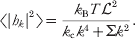
with the thermal average of the individual Fourier amplitudes immediately following from the equipartition of energy (McQuarrie, Reference McQuarrie1976; Safran, Reference Safran1994)
Assuming that height fluctuations away from h(r)=0 are small, the expression for membrane velocity is (see section 2.2)

where F(r, t)=−δH free/δh(r, t) is the force per area on the membrane resulting from the Hamiltonian H and Λ(r−r′) is the hydrodynamic kernel discussed in section 2.2. This equation follows immediately from our prior hydrodynamic analysis, if we assume that only conservative forces derived from the bending Hamiltonian and thermal random forces obeying the fluctuation–dissipation theorem (Doi & Edwards, Reference Doi and Edwards1986; Van Kampen, Reference Van Kampen2007), ζ(r′, t), act on the membrane surface.
The statistical behavior of the random force is simplest In Fourier space, where it is diagonal and obeys (Granek, Reference Granek1997)


The benefit of introducing the amplitudes h k as dynamical variables is clearly significant when using the simple Hamiltonian of equation (35), as all the modes conveniently decouple, and equation (38) simplifies to

with the wavevector-dependent relaxation frequencies

These equations describe an Ornstein–Uhlenbeck process (Van Kampen, Reference Van Kampen2007) for each mode h kwhose known analytical solutions lead to the time correlation functions


In general, more complex Hamiltonians than equation (35) will be of interest (see below). A Fourier space description is still useful in such cases for removing the real space convolution of the hydrodynamic kernel (equation (38)). The equation of motion for the h k modes can always be written

The force F k represents the transform of F(r)=−δH/δh(r, t) and is a functional of the height field h(r, t). For general Hamiltonians, F k depends on the entire set of amplitudes {h k}. i.e. Hamiltonians more complicated than equation (35) will typically lead to equations of motion that couple all of the h k modes together.
4.2 Additional harmonic forces on the membrane: application to intermembrane junctions
To this point we have focused on the case of an unperturbed membrane in solution, where analytical solution is possible. The assumption of a freely fluctuating homogeneous membrane insures a translational symmetry to the problem and leads to a Fourier decomposition as the natural normal modes for system dynamics. In principle, any Hamiltonian that is quadratic in h(r) can be solved in terms of a normal mode expansion. In practice, the number of problems that suggest an analytically tractable normal mode decomposition are somewhat limited (Fournier et al. Reference Fournier, Lacoste and Raphael2004; Granek & Klafter, Reference Granek and Klafter2001; Gov et al. Reference Gov, Zilman and Safran2004). We have suggested a numerical diagonalization procedure as a means to efficiently treat general situations involving fluid membranes coupled to harmonic perturbations (Lin & Brown, Reference Lin and Brown2004b, Reference Lin and Brown2006; Lin et al. Reference Lin and Brown2006), which has also been adopted by other workers (Merath & Seifert, Reference Merath and Seifert2006).
The technical details of the diagonalization procedure are somewhat lengthy and have been documented elsewhere (Lin & Brown, Reference Lin and Brown2004b, Reference Lin and Brown2006); they will not be repeated in detail here. The essential physical idea is, however, identical to the familiar identification of normal modes in polyatomic molecules (Atkins, Reference Atkins1990) or crystals (Aschcroft & Mermin, Reference Ashcroft and Mermin1976). Equation (35) is readily (if formally) generalized to include harmonic perturbations acting on the membrane

where the notation  ad[h(r)] is meant to convey that the additional interaction is a functional of the shape of the membrane. At present, we assume that this functional is not higher than quadratic order in h(r) (the following section deals with more general forms).

The constant C is irrelevant to the dynamics of the membrane as it only redefines the energy scale and will be dropped in what follows. In Fourier amplitudes, this is written
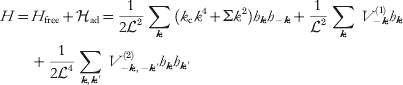
and the transformed force density, F k in equation (44) is

It should be qualitatively clear that the set of equations implied by equations (47), (48) and (44) can be solved by the introduction of a suitable linear transformation. The energy terms linear in h k (constant force terms) may be removed by completing the square and the resulting quadratic expression diagonalized through further transformation. It should also be clear that in general this transformation will need to be carried out numerically. What is perhaps not so clear is that, since h(r) is real valued and hence h k=h*−k and also that we truncate our Fourier expansion at a finite number of modes, a few additional steps (Lin & Brown, Reference Lin and Brown2004b, Reference Lin and Brown2006) must be undertaken analytically before handing these equations to the computer. As mentioned above, we will not delve into these details here, but simply reiterate that it is possible to identify a set of real-valued independent normal modes, d j, such that  and
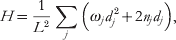

Both the n j's and v j(r)'s are given by the diagonalizing transformation. The quantities s j(t) are related to the original random forces in equation (39) and obey the fluctuation–dissipation relations


The above equations define a set of independent Ornstein–Uhlenbeck processes (Van Kampen, Reference Van Kampen2007) for the evolution of the harmonically perturbed membrane surface. As such, it is a simple matter to simulate the stochastic behavior of the membrane by drawing random numbers from suitable Gaussian distributions (Lin & Brown, Reference Lin and Brown2004b). Additionally, averages and time correlations for the eigenmodes d j can be calculated analytically in a way similar to the case of the non-interacting membrane once diagonalization has been carried out numerically. The results are


where  and h cm is the center of mass mode (k=0) for the membrane, which we have assumed stationary (Lin & Brown, Reference Lin and Brown2004b; Lin et al. Reference Lin and Brown2006) and is not included in the sum over j.
While harmonic potentials are certainly not inclusive of all interesting physical situations, they do provide us with the ability to influence membrane shape via pinning or tethering the surface to various points in 3D space. In order to constrain the membrane to pass through the point (x i, y i, z i)=(Ri, z i) we introduce the potentials


with γ a large-enough positive constant to insure the localization is enforced. Given our definitions, these choices introduce the additional potential to the free membrane
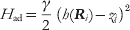

which has the effect of constraining the membrane to height z i above the position Ri in the base plane. A series of such pinning potentials can be used to mimic the geometries of experimental systems (Lin & Brown, Reference Lin and Brown2004b; Lin et al. Reference Lin and Brown2006).
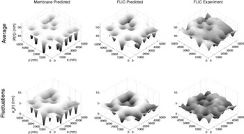
As an example of the use of harmonic pinning potentials in our modeling, we consider the case of thermal fluctuations in ‘Type-2’ (Kaizuka & Groves, Reference Kaizuka and Groves2004) intermembrane junctions (Lin et al. Reference Brannigan, Lin and Brown2006). An example of a Type-2 junction can be seen in Fig. 6. Such junctions occur experimentally when a large unilamellar vesicle is ruptured over a preexisting substrate-supported planar bilayer. The bilayer material from the vesicle adheres to the supported bilayer at a series of well-defined and immobile sites (presumably defined by defects in the underlying support matrix). This leads to an intermembrane junction with average spacing between bilayers of approximately 30–60 nm and tight adhesion at the randomly and sparsely distributed adhesion sites. The designation of ‘Type-2’ is used to differentiate such junctions from the uniformly adhered Type-1 junctions that can also occur under certain conditions (Kaizuka & Groves, Reference Kaizuka and Groves2004).
Top row: Average bilayer shape for a representative configuration of pinning sites in a Type 2 intermembrane junction. The left panel displays the predicted average membrane shape 〈h(r)〉. The middle panel displays the predicted average FLIC image 〈h m(r)〉 corresponding to the same simulation. The right panel contains the experimental FLIC data (Kaizuka & Groves, Reference Kaizuka and Groves2004). The triangle in the left image marks the location considered for dynamics as displayed in Fig. 7. Bottom row: Analogous cases to the top row, but displaying fluctuations around the average  . In all panels, the z-axis is expanded relative to x, y to emphasize detail.

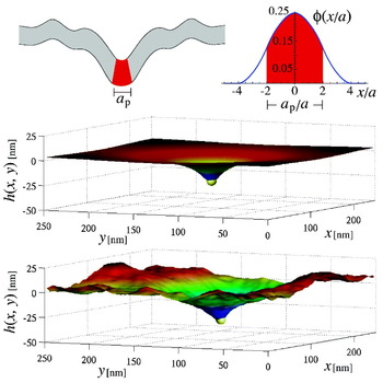
We model the upper membrane in a Type-2 junction as a C-H sheet with adhesion to the underlying bilayer provided by a series of harmonic tethering interactions. The specification of the physical pinning interaction for each adhesion site is provided by a cluster of numerical tethers (of the form of equation (56)) around the experimental defect at position R. The central tether is localized to harmonically constrain h(R)=0 (we assume that the flat supporting bilayer is found at z=0) with neighboring points in (x, y) space to this site tethered to identical heights s above the surface. The net effect of this series of tethers is to enforce an initially conical shape coming up from the substrate. It is necessary to employ such a scheme, in effect specifying the slope of the adhesion site at contact as well as the pinning depth, because the microscopic details of adhesion in Type-2 junctions are unknown; using s as a fitting parameter allows versatility in reproducing the true pinning geometry to compare with experimental results.
High-resolution time-resolved experimental data of Type-2 intermembrane junctions have been reported by Kaizuka & Groves, (Reference Kaizuka and Groves2004, Reference Kaizuka and Groves2006) using the technique of fluorescence interference contrast microscopy (FLIC). It is these data reproduced in the experimental portions of Fig. 6. The geometries inherent to a specific Type-2 junction are imposed by identifying the location of the clearly apparent adhesion sites in the experimental data and imposing numerical pins in the C-H sheet as specified in the preceding paragraph. The bilayer bending rigidity, temperature, solvent viscosity and average membrane height in the recorded region are all known experimentally. To compare with experiment, an (unnatural) periodic geometry is assumed surrounding the measured region and trial values for s and Σ are adopted. A short-wavelength cutoff in the Fourier modes is imposed at approximately 2π/85 nm−1, corresponding to the precision of the experimental data. Given the ~5·4 μm length scale of the experimental data, this leaves 64×64=4096 Fourier modes and our numerical analysis comes down to diagonalizing the 4096×4096 matrices implied by equations (47), (48) and (44). Using equations (52) evaluated at t=0 the average membrane shape and variance around this shape are immediately calculated for a chosen (s, Σ) pair. The procedure is repeated for different combinations of s and Σ to identify the best fit to experiment; the best fit results are shown in the leftmost panes of Fig. 6. (In fact, the procedure is slightly more complicated due to the diffraction limited (x, y) resolution of the experiment. The point spread function of the microscope may be taken into account to yield the middle panes of the figure (Lin et al. Reference Lin and Brown2006); it is these images compared directly to experiment).
The calculation of dynamic information requires specification of the hydrodynamic kernel. The geometry of Type-2 junctions requires that we consider a semi-infinite region of water above the membrane and a thin volume of water confined between the upper membrane and lower supported bilayer. The form of the hydrodynamic kernel is obtained by assuming identical viscosities for the fluids above and below the bilayer (i.e.  , ζ±=1 and Δ=0) in equation (26)

where d=h cm is the average height of the membrane. Note that the above expression limits to zero for k=0. This reflects the fact that the volume of water sandwiched between the two membranes is conserved; this volume is the same as h k=0=d 2. A typical time correlation function as calculated from equation (52) is displayed in Fig. 7. Again, instrument resolution makes a perceptible, though slight, modification of the physics observed in experiment.
A plot of a typical time correlation function 〈δh(r, t)δh(r, 0)〉, where δh(r, t)≡h(r, t)−〈h(r)〉, without accounting for instrumental resolution (dashed line) or δh(r, t)≡h m(r, t)−〈h m(r)〉, with the diffraction limit of light explicitly accounted for (solid line). This particular decay reflects measurement at the point indicated by the triangle in the upper-left plot in Fig. 6.

The startling thing about figure 7 is the time scale for fluctuations – approximately a tenth of a second. This number is in good agreement with experiment (Lin et al. Reference Lin and Brown2006), but is several orders of magnitude slower than would be achieved if one naively used the infinite hydrodynamic kernel of equation (24). The water in the non-confined environment above the membrane flows over distances comparable to (1/k) for each wavevector (see equation (21)); however, the water sandwiched between membrane and support is confined to the region between the two. This confinement traps the fluid and severely slows the relaxation of the membrane to which it is coupled. This case study provides a detailed comparison between experiment and elastic/hydrodynamic modeling in a complex geometry unsuited to analytical work. The influence of hydrodynamics is seen to be exceedingly strong here, influencing experimentally accessible time scales by orders of magnitude and highlighting the necessity to properly include hydrodynamic flow within simulations of membrane dynamics.
4.3 Anharmonic forces on the membrane: application to diffusion of proteins with intrinsic curvature
The methodology of the preceding section is powerful in its ability to provide a numerical (as opposed to simulation) solution to membrane dynamics. A simple matrix diagonalization provides average membrane shapes, fluctuations about this average and time correlation functions. The technique is, however, limited to problems that can be treated within a purely harmonic framework. In cases where ad[h(r)] involves arbitrary functional dependence on h(r), a genuine simulation scheme is necessary.
We have proposed a Fourier Space Brownian Dynamics (FSBD) method (Brown, Reference Brown2008; Lin & Brown, Reference Lin and Brown2004a, Reference Lin and Brown2005) for evolving membrane surfaces based on Brownian dynamics with hydrodynamic interactions (Ermak & McCammon, Reference Ermak and McCammon1978). FSBD treats the amplitudes h k as the primary dynamic variables to be stepped forward in time, much in the same way that the composition variables φk were handled in section 3. Brownian dynamics simulations are based on a discretized version of the position Langevin equation (Allen & Tildesley, Reference Allen and Tildesley1996; Ermak & McCammon, Reference Ermak and McCammon1978; Schulten & Kosztin, Reference Schulten and Kosztin2000) and FSBD is no different in this regard. In order to derive the finite-time-step version of equation (44) we simply integrate from t to t+Δt for small Δt to get


The random variable Гk(Δt), being a time integral over a Gaussian white noise, is a simple Gaussian random variable (Van Kampen, Reference Van Kampen2007). The real and imaginary parts of Гk(Δt) are both drawn from a normal distribution of mean zero and variance k BT 2Λ(k)dt at each time step. With the random numbers in hand, the amplitude of each mode is stepped forward in time by Δt by the application of equation (58). The force, F k is the Fourier transform of the real-space functional derivative of the Hamiltonian. For general cases, the force will be a complicated function in real space that is numerically transformed via FFT to k-space. The technical details have been reviewed previously (Brown, Reference Brown2008), and are discussed at length in Lin & Brown (Reference Lin and Brown2004a, Reference Lin and Brown2005, Reference Lin and Brown2006). Readers are referred to these sources for a detailed discussion.
The question of protein diffusion on curved membrane surfaces has become a subject of some interest in recent years (see Halle & Gustafsson, Reference Halle and Gustafsson1997; Naji & Brown, Reference Naji and Brown2007; Reister-Gottfried et al. Reference Reister-Gottfried, Leitenberger and Seifert2007 and references within). One well-studied consequence of membrane shape fluctuations is that a protein must travel a longer distance between two points in 3D space if the paths connecting these points are constrained to lie on a rough surface as opposed to a flat plane. This purely geometric effect is expected to have practical experimental implications; measurements that capture a 2D projection of the true motion over the membrane surface will infer diffusion coefficients of diminished magnitude relative to the intrinsic lateral diffusion locally tangent to the bilayer surface (Gov, Reference Gov2006; Halle & Gustafsson, Reference Halle and Gustafsson1997; Naji & Brown, Reference Naji and Brown2007; Reister & Seifert, Reference Reister and Seifert2005; Reister-Gottfried et al. Reference Reister-Gottfried, Leitenberger and Seifert2007). Beyond this generic effect, which should apply to anything moving on the membrane surface in relatively passive fashion (lipids, proteins, cholesterol, etc.), certain membrane-associated proteins effect shape changes in the bilayer. Specific examples include the SERC1a calcium pump (Toyoshima & Nomura, Reference Toyoshima and Nomura2002; Toyoshima et al. Reference Toyoshima, Nakasako, Nomura and Ogawa2000) and BAR (Bin, Amphiphysin, Rvs) domain dimmers (Peter et al. Reference Peter, Kent, Mills, Vallis, Butler, Evans and McMahon2004). Direct structural evidence from X-ray crystallography (Toyoshima & Nomura, Reference Toyoshima and Nomura2002; Toyoshima et al. Reference Toyoshima, Nakasako, Nomura and Ogawa2000; Peter et al. Reference Peter, Kent, Mills, Vallis, Butler, Evans and McMahon2004), experimental studies of vesicle topology at the micron scale (Girard et al. Reference Girard, Prost and Bassereau2005; Peter et al. Reference Peter, Kent, Mills, Vallis, Butler, Evans and McMahon2004) and atomically detailed simulations (Blood & Voth, Reference Blood and Voth2006) all indicate the ability of these proteins to drive membrane curvature (see Fig. 8).
An appropriately shaped protein will tend to distort the local shape of the bilayer into a bent configuration. In our simulations, the protein's effective size is defined via the envelope function in equation (62) (displayed next to the cartoon, top). The distortion is most readily seen by minimizing for the composite protein-bilayer system (middle); however, the protein's influence is strong enough to maintain visibly apparent perturbations, even in the presence of thermal fluctuations (bottom). See Table 1 for parameters.

To properly model the diffusion of curved membrane proteins requires a physical model and associated simulation algorithm capable of capturing both the passive coupling between protein diffusion and membrane shape (i.e. the geometric effect described in the preceding paragraph) as well as the direct influence of the protein on the membrane in its proximity. Our starting point is the tension-free Monge-gauge Helfrich Hamiltonian (equation (35))

where h(x)≡h(x, y) describes the local membrane displacement from a flat reference plane at z=0 (see Fig. 8). Here,  (h)=(∂xxh∂yyh−∂xyh∂xyh) is the Gaussian curvature and k c and k g are the bilayer bending modulus and saddle-splay modulus, respectively. Note that 0 is technically equivalent to H free from the last section (with ∑=0), since the apparently new Gaussian curvature term appearing in 0 actually integrates to zero. The expression has been written in this way to clearly indicate the influence of the membrane protein on the otherwise homogeneous bilayer (see equation (60)). A protein centered within the bilayer at position (R(t), h(R(t)))≡(x(t), y(t), h(x(t), y(t))) locally distorts the membrane elastic properties in the vicinity of R(t) and we assume that the total membrane Hamiltonian may be written as =0+ad with

 and
 are the protein bending and saddle-splay moduli and C p is the spontaneous curvature associated with protein shape. The protein shape function G p(r−R(t)) describes the envelope of protein influence over bilayer elastic properties. The specific function chosen has important implications for the simulations and will be discussed in detail below. For the time being, we simply comment that the function should approach a value of one at R(t) (to reflect perfect ‘protein-like’ elasticity) and should decay to zero with increasing distance from R(t) (to reflect a return to the elasticity of the homogeneous membrane sheet.
The membrane's dynamics are evolved via equation (44), with the usual truncation to N 2 modes within a periodic × box (setting the real-space mesh size at a=/N). This motion is coupled to the protein's position R(t), which may similarly be described in terms of a Langevin equation that implicitly enforces protein localization to the membrane surface (Naji & Brown, Reference Naji and Brown2007; Reister-Gottfried et al. Reference Reister-Gottfried, Leitenberger and Seifert2007). The two independent variables describing this motion are the components of R(t) (with i, j=1, 2 and summation convention assumed)

Here (g −1)ij=δij−∂ih∂jh/g is the inverse metric tensor, g=1+(∇h)2 is the determinant of the metric g ij=δij+∂ih∂jh and we have defined ∂i≡∂/∂x i. Equation (61) introduces geometric factors including v i=−[(g −1)jk∂j∂kh]∂ih/g and  (i.e. the square-root of the inverse metric tensor (g −1)ij=τikτjk). The Gaussian white-noise ηi(t) with 〈ηi(t)〉=0 and 〈ηi(t)ηj(t′)〉=δijδ(t−t′) guarantees that a tracer particle (defined by ad=0) undergoes a curvilinear random walk over the membrane surface with diffusion coefficient D 0. The last term in equation (61) reflects the effect of the interaction-induced force f i=−∂ad/∂x i.
Default parameter values used in the simulations. The protein area is chosen as Ap=(4a)2 (giving a protein diameter of ap~10 nm), the D 0 value qualitatively reflects the motion of band 3 protein dimers on the surface of human RBC (Lin & Brown, Reference Lin and Brown2004a, Reference Lin and Brown2005; Brown, Reference Brown2008), and ηw stands for the viscosity of water. For simplicity we assume that both bilayer and protein saddle-splay moduli are equal in magnitude but opposite in sign to the corresponding bending moduli

The interaction between a fully continuous variable describing protein position r(t) and a discrete representation of the membrane height field {h(xα, t)} poses certain challenges. A minor issue is that equation (61) requires the shape of the membrane surface over the entire x, y-plane and not just at the lattice sites {xα}. This problem is readily handled via linear interpolation to obtain h(x, t) and the required derivatives at arbitrary x from the corresponding neighboring lattice values (Reister-Gottfried et al. Reference Reister-Gottfried, Leitenberger and Seifert2007). A more complex problem involves the dynamics of the h k(t)'s in equation (58). The forces in this equation include contributions due to the coupling between protein and bilayer from equation (60). The envelope function G p(x) reflects protein size and is quite localized in real space; the natural way to deal with equation (60) (and the related force expressions) is to approximate the integral by simple quadrature, i.e.  for arbitrary function . To define a numerical scheme that is both efficient and accurate, the specific functional form chosen for G p is critical. Naive continuous choices like 2D Gaussians (Brown, Reference Brown2008; Leitenberger et al. Reference Leitenberger, Reister-Gottfried and Seifert2008; Lin & Brown, Reference Lin and Brown2004a, Reference Lin and Brown2005), for example, lead to an effective normalization (as computed by quadrature) that varies with the offset between the envelope center and the discrete lattice. Piecewise linear forms for G p can be defined that suffer no such normalization issue, but such functions lead to discontinuous derivatives as the protein–lattice offset changes.
From a numerical perspective, the ‘correct’ choice for the functional form of G p(x), which avoids these difficulties, has been identified previously (Peskin, Reference Peskin2002) and we adopt this choice here (Naji et al. Reference Naji, Atzberger and Brown2009). We take G p(x)=(A p/a 2)φ(x/a)φ (y/a) with (Peskin, Reference Peskin2002) (see Fig. 8 for a plot)
and zero for all other u values. A p defines an effective protein area and the envelope function is non-vanishing over a total of 64 lattice sites. Choices involving a significantly smaller support region are possible (e.g. 16 lattice sites); equation (62) insures fully converged results for all of the cases considered in this work. In order to simulate the dynamics of the system, we evolve equations (58) and (61) in time via the Euler–Maruyuma method (Kloeden & Platen, Reference Kloeden and Platen1992). Adopting the envelope function defined in equation (62) allows a seamless melding of the approaches introduced (Brown, Reference Brown2008; Lin & Brown, Reference Lin and Brown2004a, Reference Lin and Brown2005; Naji & Brown, Reference Naji and Brown2007; Reister-Gottfried et al. Reference Reister-Gottfried, Leitenberger and Seifert2007). In the simulations, we use =250 nm and N=100 giving a=2·5 nm, which is compaarble to bilayer thickness. The protein area is chosen as A p=(4a)2=100 nm2 giving a size (diameter) of a p~10 nm. Membrane bending rigidity is set to k c/(k BT)=5, temperature to T=300 K and the bare diffusion coefficient for the protein to D 0=5·0 μm2/s, qualitatively reflecting the motion of band 3 protein dimers on the surface of human RBC (Brown, Reference Brown2008; Lin & Brown, Reference Lin and Brown2004a, Reference Lin and Brown2005). We allowed the viscosity of the medium, the protein bending modulus and the protein spontaneous curvature to vary over the ranges η=0·001 (water) to 0·006 Pa⋅s (RBC cytoplasm),  to 8 and C p=0·025 nm−1 to 0·15 nm−1, respectively. For simplicity, it was assumed that both bilayer and protein saddle-splay moduli were equal in magnitude but opposite in sign to the corresponding curvature moduli, i.e. K′m(p)=−K m(p). The projected diffusion coefficient, D, is calculated as
 . The simulations run for ~5×10⁷ time steps of size ~0·01 ns, ensuring both numerical accuracy and statistically reliable results.
The protein's influence on the membrane is most easily seen in the absence of thermal shape fluctuations of the membrane, but for sufficiently large C p and values the effect of the protein remains clearly visible despite thermal fluctuations of the membrane surface (see Fig. 8). The average distortion of the membrane surrounding the protein is sufficient to significantly slow protein motion in all cases we have studied (see Fig. 9). This slowing derives from two effects. First, the protein tends to trap itself in the deformation created by its own perturbation to the bilayer. The energy-minimized configuration displayed in Fig. 8 places the protein at the bottom of a curved valley; attempted diffusion up the walls of this valley is hindered by the interaction-induced force in equation (61). Second, x, y translation of the protein is accompanied by translation of the membrane deformation surrounding this protein. The hydrodynamic effects included in equation (58) dictate that the translation of such a deformation is resisted by the viscous drag of the medium surrounding the bilayer. This drag acts in addition to the usual quasi-2D drag incorporated within D 0 and slows protein motion. These effects are most pronounced when shape fluctuations of the bilayer are neglected by setting T=0 in equation (58). Increasing the local deformation around the protein or the solvent viscosity both decrease D. In Fig. 9, we display three means to control this effect. Increasing C p drives large deformations from a flat plane for any finite . Larger values of will tend to increase this effect up until the point where the rigidity of the protein becomes effectively infinite and the response to the protein saturates. The hydrodynamic drag in our model is controlled via η; increases in η reduce D as effectively as do perturbations to membrane shape.
Projected diffusion coefficients for protein motion over an elastic membrane. In each panel, one of the three parameters (protein bending modulus), C p (protein spontaneous curvature) and η (medium viscosity) is varied as indicated while holding the remaining physical properties at the default values indicated in Table 1. Circles indicate the results of full simulations including thermal motion of both the bilayer and the protein. The triangles indicate results obtained by turning off all bilayer shape fluctuations (i.e. setting T=0 for membrane undulations modes) and the solid squares indicate the results of the adiabatic theory discussed in the text. Insets show simulation results obtained within the asymmetric coupling approximation. Error bars are approximately the size of the symbols. Diffusion coefficients are calculated as  . The simulations run for ~5×10⁷ time steps of size Δt~0·01 ns, ensuring both numerical accuracy and statistically reliable results. The protein's root-mean-square displacements over the course of the simulations are approximately 100 nm (i.e. 20 times the protein's radius).

Within the asymmetric coupling approximation, which ignores the influence of the protein on membrane shape, it is predicted that bilayer shape fluctuations will enhance curved protein mobility (Leitenberger et al. Reference Leitenberger, Reister-Gottfried and Seifert2008; Reister & Seifert, Reference Reister and Seifert2005) (i.e. D>D 0, insets in Fig. 9). Although this effect can be seen in our simulations, the enhancement in diffusivity due to thermal fluctuations is slight (relative to the similar effect within the aforementioned approximation scheme) and cannot overcome the dominant slowing caused by the protein's distortion of the bilayer (compare open circles and triangles, Fig. 9). We find D<D 0 for all cases studied.
In order to demonstrate the role of hydrodynamics more clearly in these results, we can interpret the observed trends with a simplified analytical model. We have argued above that the drag associated with the protein-induced membrane deformation will act to slow protein motion. If we assume that this deformation is (at least on average) well approximated by the energy-minimized membrane distortion seen in the middle panel of Fig. 8, we can readily predict its effect on D. We denote this minimized shape profile as  (x, t) and assume that the profile instantaneously adjusts to the position of the protein. It then follows that

for a protein moving at constant lateral velocity v. The power dissipated by viscous losses in the medium may be calculated from  , where F k(t) follows from equation (44) as
 . Therefore, the power loss may be written as
 with μdef being the effective mobility of the deformation. The effective protein diffusion coefficient follows from D def=μdefk BT and D −1=(D 0−1+D def−1) to give

This expression depends only on the minimized deformation profile of the membrane at fixed protein position, which is readily calculated numerically. The results of equation (64) are shown alongside the simulation results in Fig. 9. Although the approximation is imperfect due to the neglect of membrane shape fluctuations and the self-trapping effect discussed above, the results serve as a reliable estimator of the observed trends for the full simulation. Further, since equation (64) results from the estimation of hydrodynamic drag on the protein-induced membrane deformation without any other considerations, it seems clear that hydrodynamic effects dominate the slowing seen in the simulations.
Unlike the previous examples considered in this review, the results of this section have not been tested experimentally (at least not to our knowledge); however, it would seem rather straightforward to do so. We do note that recent experiments (Gambin et al. Reference Gambin, Lopez-Esparza, Reffay, Sierecki, Gov, Genest, Hodges and Urbach2006, Reference Gambin, Reffay, Sierecki, Homble, Hodges, Gov, Taulier and Urbach2010; Ramadurai et al. Reference Ramadurai, Holt, Schafer, Krasnikov, Rijkers, Marrink, Killian and Poolman2010a, Reference Ramadurai, Duurkens, Krasnikov and Poolmanb) have called into question the traditional SD results (Saffman & Delbrück, Reference Saffman and Delbrück1975) for membrane-protein diffusion (however, some of these results are controversial (Ramadurai et al. Reference Ramadurai, Holt, Krasnikov, van den Bogaart, Killian and Poolman2009)). It seems that the measurement of membrane-protein diffusivities is becoming more popular and we are optimistic that careful experimental studies of D for curved proteins may soon become available. A particularly striking prediction of this work is the strong dependence of D on the viscosity of the bulk fluid (in contrast to the weak logarithmic dependence predicted for flat proteins (Saffman & Delbrück, Reference Saffman and Delbrück1975)), which could perhaps be observed experimentally.
5. Conclusion
The continuum picture of fluid membrane sheets as embodied by the Canham–Helfrich (Canham, Reference Canham1970; Helfrich, Reference Helfrich1973) model for membrane shape energetics, and the hydrodynamic models of Brochard & Lennon (Reference Brochard and Lennon1975) and Saffman & Delbrück (Reference Saffman and Delbrück1975) for out-of-plane and in-plane membrane dynamics, respectively, were developed close to 40 years ago. The fact that these models are still widely applied today represents a true testament to the vision of these workers and the power of their theories. The work reviewed above represents a collection of tools and applications related to the use of these theories in a simulation setting.
The successes described above are gratifying to see and illustrate that it is possible to make direct connection between biophysical experiment and theory, even when experimental observations are restricted to the micron/second scales accessible to optical microscopy. Continuum models do have fundamental limitations however. The physical parameters appearing as inputs to these theories must be obtained elsewhere, either from experiment or from more detailed simulations. And the continuum models themselves will break down if applied to length and time regimes outside their regimes of validity. Continuum models and more detailed particle-based approaches are complementary to one another, with particle-based approaches resolving molecular scale detail and continuum approaches explaining the collective behavior of large assemblies of these molecules.
Before concluding, it is worth mentioning some of the many possible extensions to the work discussed above. Some of these extensions are under active development within our group and others will be considered shortly. All of these extensions are related to extending the applicability of the continuum approach to a broader class of experiments and phenomena in membrane biophysics.
An obvious extension to the simulations discussed above would be the melding of the models introduced in sections 3 and 4 to allow the study of composition dynamics over non-flat geometries and the incorporation of protein motion and inhomogeneous lipid environments within the same model. Phase segregation and membrane shape can be strongly coupled for appropriately chosen lipids (Webb et al. Reference Webb, Barak, Tank and Wu1981) and the interaction between proteins and lipid phases may have important implications for the behavior of lipid rafts. The decoupling between in-plane and out-of-plane dynamics (for sufficiently small deviations from flatness) (Levine & MacKintosh, Reference Levine and MacKintosh2002) makes such an extension quite straightforward. The primary difficulty here lies in obtaining the additional physical parameters necessary to completely specify such a generalized model; we are currently working in this direction.
Experimentally, bilayer systems are commonly studied as vesicles. Our modeling in terms of a flat sheet is appropriate only for studying the behavior of such systems at length scales significantly smaller than the vesicle diameter. It is possible to extend our numerical techniques beyond the Monge gauge, to the study of quasi-spherical geometries by expanding the bilayer shape in spherical harmonics as opposed to Fourier modes (Milner & Safran, Reference Milner and Safran1987). In fact, we have already conducted preliminary simulations of this sort, but the numerics are not as efficient as for the plane. The existence of highly optimized and well-established FFT software packages (http://wwww.fftw.org) is key to the success of our prior modeling efforts; extending our codes to spherical geometries, while retaining similar numerical efficiency to the planar case, represents a practical challenge we are currently working to overcome.
Our treatment of dynamics has assumed that the dominant source of drag acting against membrane undulations is the flow of solvent outside the bilayer. In fact, it has been suggested theoretically (Seifert & Langer, Reference Seifert and Langer1993) and recently confirmed via simulation (Shkulipa et al. Reference Shkulipa, den Otter and Briels2006) and experiment (Lee et al. Reference Lee, Choi, Doe, Faraone, Pincus and Kline2010; Watson & Brown, Reference Watson and Brown2010) that bulk solvent viscosity is less important than inter-monolayer friction and monolayer surface viscosity for determining membrane shape dynamics at small (tens of nanometers and less) length scales. The applications discussed in this review are largely insensitive to the dynamics at these wavelengths and our current level of modeling should be appropriate. More generally, to properly model short-wavelength behavior (though still long enough to justify a continuum approach) it is necessary to adopt a more refined picture of the membrane accounting for the coupling between monolayers. It is possible to include the leaflet structure of the membrane with minimal changes to the approach discussed in section 4; however, an additional field is needed to track the local lipid density mismatch between the two leaflets (the sheets are compressible within the standard model for these effects (Seifert & Langer, Reference Seifert and Langer1993)). Such an approach could certainly be pursued, but we mention that the continuum-level energetics of membranes become increasingly complicated when short wavelength and the dual-leaflet structure are explicitly considered (Brannigan & Brown, Reference Brannigan and Brown2006, Reference Brannigan and Brown2007; West et al. Reference West, Brown and Schmid2009). It is not yet clear as to what level of detail must be employed in the energetics of these systems to obtain a robust model for membrane dynamics at resolutions finer than those considered in this work. This is certainly a topic worthy of further study, especially considering the recent measurement of experimental membrane dynamics down to wavelengths comparable to bilayer thickness (Nagao, Reference Nagao2009).
Finally, although the focus of this review was on hydrodynamic effects at the membrane surface, the assumed Newtonian behavior of both the bulk solvent and the membrane may need to be relaxed for certain applications. Even model membrane systems can exhibit signatures of viscoelasticity (Crawford & Earnshaw, Reference Crawford and Earnshaw1987; Harland et al. Reference Harland, Bradley and Parthasarathy2010) and cellular cytoplasm with cytoskeletal structure and all manner of complex molecules crowded within it cannot be expected to behave as a simple fluid. The standard linear constitutive laws for viscoelasticity (Ferry, Reference Ferry1980; Levine & MacKintosh, Reference Levine and MacKintosh2002; Squires & Mason, Reference Squires and Mason2010; Xu & Klapper, Reference Xu and Klapper2007) could be incorporated within the models discussed here (albeit with additional computational expense), but it is very unclear that real biological systems could be treated within such a framework. It may be necessary to introduce such models in the simulation of model membrane systems, but it remains to be seen to what extent viscoelasticity affects the dynamics of lipid bilayers experimentally.
Of course, the above technical issues would be of little interest without clearly defined biological and/or biophysical motivating questions to answer. The extensions briefly discussed above should enable the study of many questions involving the interaction between membrane surfaces and other cellular structures. Problems related to cellular motility (Theriot & Mitchison, Reference Theriot and Mitchison1991; Howard, Reference Howard2001), lipid raft structure and dynamics (Simons & Vaz, Reference Simons and Vaz2004b; Fan et al. Reference Fan, Sammalkorpi and Haataja2010) and the formation of biologically relevant intermembrane junctions (Grakoui et al. Reference Grakoui, Bromley, Sumen, Davis, Shaw, Allen and Dustin1999) all seem amenable to such an approach. Although the theory for continuum membranes is decades old, we have just begun to scratch the surface for application of these ideas to the more complex systems relevant to biology and amenable to simulation studies.
6. Acknowledgements
I thank Paul Atzberger, Brian Camley, Lawrence Lin, Ali Naji and Max Watson for their contributions to the work discussed herein, which has been supported by the National Science Foundation (grant nos. CHE-0349196, CHE-0321368 and CHE-0848809) and the US–Israel binational science foundation (grant no. 2006285). The author is a Camille Dreyfus Teacher-Scholar and was an Alfred P. Sloan Research Fellow when much of this work was originally carried out.