





1. Introduction
Let Hk be the set of normalized primitive holomorphic cusp forms of even integral weight k for the full modular group  $SL(2,\mathbb{Z})$, which are eigenfunctions of all the Hecke operators Tn. Then
 $f(z) \in H_{k}$ has a Fourier expansion at the cusp infinity
 \begin{equation*}
f(z)=\sum\limits_{n=1}^{\infty}\lambda_{f}(n)
n^{\frac{k-1}{2}}e(nz) \quad (\Im z \gt 0),
\end{equation*}
where we normalize f(z) so that  $\lambda_{f}(1)=1$. From the theory of Hecke operators, the coefficient
 $\lambda_{f}(n)$ is real and satisfies the multiplicative property
 \begin{equation}
\lambda_{f}(m)\lambda_{f}(n)=\sum_{d|(m,n)}\lambda_{f}\left(\frac{mn}{d^{2}}\right),
\end{equation}
where  $m\geqslant 1$ and
 $n \geqslant 1$ are any integers. In 1974, Deligne [Reference Deligne2] proved the Ramanujan–Petersson conjecture: for all integers
 $n\geqslant 1$,
 \begin{equation*}
|\lambda_{f}(n)|\leqslant d(n),
\nonumber
\end{equation*}
where d(n) is the number of positive divisors of n.
The Hecke L-function attached to f is given by
 \begin{equation*}
L(s, f)=\sum_{n=1}^{\infty} \frac{\lambda_{f}(n)}{n^{s}}= \prod_{p}\left(1-\frac{\alpha_{f}(p)}{p^{s}}\right)^{-1}\left(1-\frac{\beta_{f}(p)}{p^{s}}\right)^{-1},
\nonumber
\end{equation*}
which converges absolutely for  $\Re(s) \gt 1$. The local parameters
 $\alpha_{f}(p)$ and
 $\beta_{f}(p)$ satisfy
 \begin{equation}
\alpha_{f}(p)+ \beta_{f}(p) =\lambda _f (p)\quad \text{and}\quad
\alpha_{f}(p) \beta_{f}(p)=|\alpha_{f}(p)|=| \beta_{f}(p)| = 1.
\end{equation}
Associated to  $f(z) \in H_{k}$, the jth symmetric power L-function is defined as
 \begin{align}
L(s,\mathrm{sym}^{j}f)&=\prod_{p} \prod_{m=0}^{j}\left(1-\alpha_{f}(p)^{j-m} \beta_{f}(p)^{m} p^{-s}\right)^{-1}\nonumber\\
&:=\sum_{n=1}^{\infty} \frac{\lambda_{\mathrm{sym}^{j} f}(n)}{n^{s}},
\qquad for ~\ \Re(s) \gt 1,
\end{align}
where  $\lambda_{\mathrm{sym}^{j}f}(n)$ is a real multiplicative function and
 $ L\left(s,\mathrm{sym}^{0}f\right)=\zeta(s)$.
According to the Langlands program, the most general L-function should be a product of L-functions of automorphic cuspidal representations of  $GL_{m}/\mathbb{Q}$. Therefore these automorphic L-functions do deserve deep investigation. The symmetric square L-function is an important automorphic L-function. As a result, the average behavior of the Fourier coefficients of
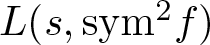
 $L(s,\mathrm{sym}^{2} f)$ is an important subject in analytic number theory and it has received much attention. Let
 \begin{equation*}
M_{j}(x):=\sum\limits_{n\le x} \lambda _{\mathrm{sym}^{2}f}^{j}(n) , \qquad j\in \mathbb{N}^{+}.
\nonumber
\end{equation*}
Fomenko [Reference Fomenko3] first studied the sum of  $\lambda _{\mathrm{sym}^{2}f}(n)$ and established that
 \begin{equation*}
M_{1}(x)\ll x^{1/2}\log ^{2}x.
\nonumber
\end{equation*}
After that, there have been extensive study of this sum (see Ichihara [Reference Ichihara8], Jiang–Lü [Reference Jiang and Lü11], Lü [Reference Lü12], Lü-Tang [Reference Lü and Tang13], Sankaranarayanan [Reference Sankaranarayanan24], Tang [Reference Tang27]). The best current known bound, proved by Tang–Wu [Reference Tang and Jie25], is
 \begin{equation*}
M_{1}(x)\ll x^{1/2}(\log x)
^{-(1-\frac{3\sqrt{3}}{2\pi})}
.
\nonumber
\end{equation*}
Then, the higher moment of the Fourier coefficients of  $L(s,\mathrm{sym}^{2} f)$ has been researched by many scholars. Fomenko [Reference Fomenko4] showed that
 \begin{equation*}
M_{2}(x)=c_{2}x+O(x^{\gamma}),
\nonumber
\end{equation*}
where  $c_{2} \gt 0$ is a suitable constant depending on f and γ < 1 is a constant. Later, Tang [Reference Tang26] improved the error term to
 $O(x^{10/13}\log ^{9}x)$. Lao [Reference Lao14] studied the fourth moment of coefficients of symmetric square L-function and proved that
 \begin{align*}
M_{4}(x) = x P_{4}( \log x ) + O( x^{79/
81+\epsilon}),
\end{align*}
where  $P_{4}(t)$ is a polynomial in t of degree 2. Afterwards, He [Reference Xiaoguang28] improved the error term of the above results with
 $j=2,4$ and studied the result with j = 3 by demonstrating that
 \begin{align*}
M_{j}(x) = xP_{j}(\log x) + O(x^{\delta_{j}+\epsilon}), \qquad \text{for }j= 2,3,4,
\end{align*}
where  $P_{j}(t)$ is a polynomial in t with
 $\operatorname{deg} P_{2}(t)=\operatorname{deg} P_{3}(t)=0$,
 $\operatorname{deg} P_{4}(t)=2$, and
 $\delta_{2}=13/17$,
 $\delta_{3}= 248/
269 $,
 $\delta_{4}=3223/3307$.
Recently, the result of Newton–Thorne [Reference Newton and Thorne22] implies that  $\mathrm{sym}^{j}f$ (
 $j\in \mathbb{N}^{+}$) is an automorphic cuspidal representation of
 $GL(j+1)$. Applying this property, Luo-Lao-Zou [Reference Luo, Lao and Zou21] considered more general cases for
 $3\leqslant j \leqslant 8$ and improved the previous average formula on error term. In [Reference Liu20], giving new decompositions for the Dirichlet series, using the new subconvexity result for the symmetric square L-function and shifting the contour of the integration to a different line from [Reference Luo, Lao and Zou21], Liu further improved the results of Luo-Lao-Zou by showing that
 \begin{equation*}
M_{j}(x)=xP_{j}(\log x)+O\left(x^{\theta _{j}+\varepsilon}\right),\qquad j=3,4,5,6,7,8,
\nonumber
\end{equation*}
where  $P_{j}(t)$ is a polynomial in t with
 $\operatorname{deg} P_{3}(t)=0$,
 $\operatorname{deg} P_{4}(t)=2$,
 $\operatorname{deg} P_{5}(t)=5$,
 $\operatorname{deg} P_{6}(t)=14$,
 $\operatorname{deg} P_{7}(t)=35$ and
 $\operatorname{deg} P_{8}(t)=90$, with
 \begin{align*}
\theta_{3}&=\frac{1367}{1487},\qquad \theta_{4}=\frac{1483}{1523},\qquad \theta_{5}=\frac{459}{463},\\
\theta_{6}&=\frac{12237}{12272},\qquad \theta_{7}=\frac{74069}{74139},\qquad \theta_{8}=\frac{335197}{335302}.
\end{align*}
In this paper, we consider the sum  $M_{j}(x)$ for
 $j\geqslant 3$, and get some new results which improve the previous results. We have the following results.
Theorem 1. Let  $f \in H_{k}$ and
 $\lambda_{\mathrm{sym}^{2}f}(n)$ be the
 $\mathrm{Fourier}$ coefficient of
 $L(s,\mathrm{sym}^{2}f)$. Then for any ɛ > 0, we have
 \begin{equation*}
M_{3}(x)=cx+O\left(x^{\frac{2933}{3193}+\varepsilon}\right),
\nonumber
\end{equation*}
where c > 0 is a constant depending on f.
Theorem 2. Let  $f \in H_{k}$ and
 $\lambda_{\mathrm{sym}^{2}f}(n)$ be the
 $\mathrm{Fourier}$ coefficient of
 $L(s,\mathrm{sym}^{2}f)$. Then for any ɛ > 0, we have
 \begin{equation*}
M_{j}(x)=xP_{j}(\log x)+O\left(x^{1-\theta _{j}+\varepsilon}\right),\qquad j=4,5,6,7,8,
\nonumber
\end{equation*}
where  $P_{j}(t)$ is a polynomial in t with
 $\operatorname{deg} P_{4}(t)=2$,
 $\operatorname{deg} P_{5}(t)=5$,
 $\operatorname{deg} P_{6}(t)=14$,
 $\operatorname{deg} P_{7}(t)=35$ and
 $\operatorname{deg} P_{8}(t)=90$, with
 \begin{align*}
\theta_{4}&=\frac{105}{3946},\qquad
\theta_{5}=\frac{63}{8\sqrt{30}+7182},\qquad
\theta_{6}=\frac{1155}{200\sqrt{66}+399861},\nonumber\\
\theta_{7}&=\frac{455}{160\sqrt{65}+476931},\qquad
\theta_{8}=\frac{315}{520\sqrt{14}+997101}.\nonumber
\end{align*}
Theorem 3. Let  $f \in H_{k}$ and
 $\lambda_{\mathrm{sym}^{2}f}(n)$ be the
 $\mathrm{Fourier}$ coefficient of
 $L(s,\mathrm{sym}^{2}f)$. Then for any ɛ > 0, we have
 \begin{equation*}
M_{j}(x)=
xP_{j}(\log x) +O\left(x^{1-\theta_{j}+\epsilon}\right)
,\qquad j\geqslant 9,
\nonumber
\end{equation*}
where  $P_{j}(t)$ is a polynomial in t with
 \begin{align*}
\operatorname{deg} P_{j}(t)=\sum\limits_{k=0}^{j}(-1)^{j-k}
C_{k}
\left(\begin{matrix}
j\\k
\end{matrix}\right)
-1.
\end{align*}
and
 \begin{equation*}\theta_{j}=1/k_{j},\end{equation*}
with
 \begin{align*}
k_{j}=&
\frac{8}{63}\sqrt{\frac{15}{2j-1}}
\left(
\sum\limits_{k=0}^{j}(-1)^{j-k}C_{k}
\left(\begin{matrix}
j\\k
\end{matrix}\right)
\right)
+\frac{6}{5}
\left( \sum\limits_{k=1}^{j}(-1)^{j-k}
\left(\begin{matrix}
j\\k
\end{matrix}\right)
\left(
\left(\begin{matrix}
2k\\k-1
\end{matrix}\right)
-
\left(\begin{matrix}
2k\\k-2
\end{matrix}\right)
\right)\right)
\nonumber\\
&
+\sum_{t=2}^{j}
\left(
\sum\limits_{k=t}^{j}(-1)^{j-k}
\left(\begin{matrix}
j\\k
\end{matrix}\right)
\left(
\left(\begin{matrix}
2k\\k-t
\end{matrix}\right)
-
\left(\begin{matrix}
2k\\k-t-1
\end{matrix}\right)
\right) \right)
\frac{2t+1}{2}.
\end{align*}
For a random variable X defined on a countable sample space  $\mathbb{V}$, we define E(X) and
 $\text{Var}(X)$ as the mathematical expectation and variance of X, respectively. Applying Theorem 1, Theorem 2, Theorem 3 and the variance formula [Reference Chung and AitSahlia1, Theorem 3]
 \begin{equation}
\text{Var}(X)=E(X^{2})-E^{2}(X),
\end{equation}
as in [Reference Luo, Lao and Zou21, p.255], we can obtain the asymptotic formula of the variances of  $\lambda _{\mathrm{sym}^{2}f}^{j}(n)$ for
 $1 \leqslant n \leqslant x$, denoted by
 \begin{equation*}
\text{Var}
\left ( \lambda _{\mathrm{sym}^{2}f}^{j}(n)\right)_{1\leqslant n\leqslant x}
,
\end{equation*}
in the following corollary.
Corollary 1. Under previous notations, we have for  $j\geqslant 3$
 \begin{equation*} \text{Var}
\left ( \lambda _{\mathrm{sym}^{2}f}^{j}(n)\right)_{1\leqslant n\leqslant x}={Q}_{2j}(\log x)+O\left(x^{-\theta _{2j}+\varepsilon}\right),\end{equation*}
where  $Q_{2j}(t)$ is a polynomial in t with
 \begin{align*}
\operatorname{deg} Q_{2j}(t)=\sum\limits_{k=0}^{2j}(-1)^{2j-k} C_{k}
\left(\begin{matrix}
2 j\\k
\end{matrix}\right)
-1,
\end{align*}

Automorphic form is one of the central topics in the field of analytic number theory. It is of interest to investigate the Fourier coefficients of the holomorphic cusp form. Motivated by He’s work [Reference Xiaoguang28], we consider the sum
 \begin{equation*}
S_{l}(x):=\sum\limits_{n\le x} \lambda _{f}^{l}(n^{2}),\nonumber
\end{equation*}
where  $\lambda _{f}(n)$ is the nth normalized Fourier coefficient of holomorphic Hecke eigenform
 $f(z)\in H_{k}$. This problem is an interesting subject in number theory, as we observe that the average behaviour of
 $S_{l}(x)$ closely resembles that of
 $M_{j}(x)$.
For l = 2, the estimate of  $S_{2}(x)$ began with Lao–Sankaranarayanan [Reference Lao and Sankaranarayanan16] and continued with Lao–Sankaranarayanan [Reference Lao and Sankaranarayanan17], Lao-Mckee-Ye [Reference Lao, McKee and Yangbo15] and He [Reference Xiaoguang28].
For l = 3, He [Reference Xiaoguang28] proved that
 \begin{equation*}
S_{3}(x)=\tilde{c}x+O\left(x^{\frac{248}{269}+\varepsilon}\right),
\nonumber
\end{equation*}
where  $ \tilde{c} \gt 0$ are some constants depending on f.
For l = 4, the first result was proved by Lao [Reference Lao14], and the up-to-date result is due to He [Reference Xiaoguang28] by showing that
 \begin{equation*}
S_{4}(x)=x\tilde{P}(\log x)+O\left(x^{\frac{3223}{3307}+\varepsilon}\right),
\nonumber
\end{equation*}
where  $\tilde{P}(t)$ is a polynomial in t of degree 2.
In this paper, we also investigate the sum  $S_{l}(x)$ for more general cases
 $l\geqslant 3$ and get some new results which improve the previous error term estimate. We have the following results.
Theorem 4. Let  $f \in H_{k}$ and
 $\lambda_{f}(n)$ be the
 $\mathrm{Fourier}$ coefficient of
 $\textstyle f(z)$. Then for any ɛ > 0, we have
 \begin{equation*}
\sum\limits_{n\le x} \lambda _{f}^{l}(n^{2})=x\tilde{P}_{l}(\log x)+O\left(x^{1-\tilde{\theta} _{l}+\varepsilon}\right),\qquad l=3,4,5,6,7,8,
\nonumber
\end{equation*}
where  $\tilde{P}_{j}(t)$ is a polynomial in t with
 $\operatorname{deg} \tilde{P}_{3}(t)=0$,
 $\operatorname{deg} \tilde{P}_{4}(t)=2$,
 $\operatorname{deg} \tilde{P}_{5}(t)=5$,
 $\operatorname{deg} \tilde{P}_{6}(t)=14$,
 $\operatorname{deg} \tilde{P}_{7}(t)=35$ and
 $\operatorname{deg} \tilde{P}_{8}(t)=90$, with
 \begin{align*}
\tilde{\theta}_{3}&=\frac{260}{3193},\qquad
\tilde{\theta}_{4}=\frac{105}{3946},\qquad
\tilde{\theta}_{5}=\frac{63}{8\sqrt{30}+7182},\qquad
\tilde{\theta}_{6}=\frac{1155}{200\sqrt{66}+399861},\nonumber\\
\tilde{\theta}_{7}&=\frac{455}{160\sqrt{65}+476931},\qquad
\tilde{\theta}_{8}=\frac{315}{520\sqrt{14}+997101}.\nonumber
\end{align*}
Theorem 5. Let  $f \in H_{k}$ and
 $\lambda_{f}(n)$ be the
 $\mathrm{Fourier}$ coefficient of
 $\textstyle f(z)$. Then for any ɛ > 0, we have
 \begin{equation*}
\sum\limits_{n\le x} \lambda _{f}^{l}(n^{2})=x\tilde{P}_{l}(\log x)+O\left(x^{1-1/ \tilde{k} _{l}+\varepsilon}\right),\qquad l\geqslant 9,
\nonumber
\end{equation*}
where  $\tilde{P}_{l}(t)$ is a polynomial in t with
 \begin{align*}
\operatorname{deg} \tilde{P}_{l}(t)=\sum\limits_{k=0}^{l}(-1)^{l-k} C_{k}
\left(\begin{matrix}
l\\k
\end{matrix}\right)
-1.
\end{align*}
and
 \begin{align*}
\tilde{k}_{l}& =
\frac{8}{63}\sqrt{\frac{15}{2l-1}}
\left(
\sum\limits_{k=0}^{l}(-1)^{l-k} C_{k}
\left(\begin{matrix}
l\\
k
\end{matrix}\right)
\right)
+\frac{6}{5}
\left( \sum\limits_{k=1}^{l}(-1)^{l-k}
\left(\begin{matrix}
l\\
k
\end{matrix}\right)
\left(
\left(\begin{matrix}
2k\\
k-1
\end{matrix}\right)
-
\left(\begin{matrix}
2k\\
k-2
\end{matrix}\right)
\right)\right)
\nonumber\\
& \quad
+\sum_{t=2}^{l}
\left(
\sum\limits_{k=t}^{l}(-1)^{l-k}
\left(\begin{matrix}
l\\
k
\end{matrix}\right)
\left(
\left(\begin{matrix}
2k\\
k-t
\end{matrix}\right)
-
\left(\begin{matrix}
2k\\
k-t-1
\end{matrix}\right)
\right) \right)
\frac{2t+1}{2}.
\nonumber
\end{align*}
Remark 1. Comparing Lemma 1-Lemma 5, we find that the proof of Theorem 4 and Theorem 5 are similar to those of Theorem 1, Theorem 2 and Theorem 3, so we omit them here.
Remark 2. For our results, the improvement is based on the new results on the individual and averaged subconvexity bounds for  $\zeta(s)$ and the symmetric power L-function
 $L(s,\mathrm{sym}^{j} f)$. A different shift of the line of the corresponding integration to [Reference Xiaoguang28] [Reference Liu20] and applying optimal choices of Hölder inequalities also play important roles in the improvement. Last but not least, we propose a new decomposition of
 $L_{j}(s)$ and
 $G_{j}(s)$ for
 $j\geqslant 9$ (see Lemma 3 and Lemma 5), which is central to the proof of Theorem 3 and Theorem 5.
In Sect.2, we give some preliminary lemmas. In Sect.3 - Sect.6, we complete the proofs of Theorem 1 - Theorem 3, Corollary 1, respectively. And, throughout the paper, we denote by ϵ a sufficiently small positive constant, whose value may not be necessarily the same in all occurrences. The symbol  $\left(\begin{matrix}
a\\b
\end{matrix}\right)$ is the binomial coefficient with the convention that
 $\left(\begin{matrix}
0\\0
\end{matrix}\right)=1$ and
 $\left(\begin{matrix}
a\\b
\end{matrix}\right)=0$ if b < 0. The symbol Ck is the Catalan number, which is equal to
 $\left(\begin{matrix}
2k\\k
\end{matrix}\right)-
\left(\begin{matrix}
2k\\k-1
\end{matrix}\right).$
2. Preliminaries and some lemmas
In this section, we will recall or establish some lemmas to prove our theorems.
Lemma 1. Let  $f \in H_{k}$ and
 $\lambda_{\mathrm{sym}^{2}f}(n)$ denote the Fourier coefficient of the symmetric square
 $L$-function. Set
 \begin{equation*}
L_{3}(s)=\sum_{n=1}^{\infty}\frac{\lambda^{
3
}_{ \mathrm{sym}^{2}f }(n)}{n^{s}}, \qquad \text{for }\Re (s) \gt 1. \nonumber
\end{equation*}
Then, we have
 \begin{equation*}
{L}_{3}(s)= \zeta(s) L^{3}(s,\mathrm{sym}^{2}f) L^{2}(s,\mathrm{sym}^{4}f) L(s,\mathrm{sym}^{6}f)U_{3}(s),
\nonumber
\end{equation*}
where  $U_{3}(s)$ converges uniformly and absolutely in the half-plane
 $\Re(s) \geqslant $
 $1 / 2+\varepsilon$ for any ɛ > 0, and is defined as Lemma 2.1 in [Reference Luo, Lao and Zou21].
Proof. See [Reference Luo, Lao and Zou21, Lemma 2.1] .
Lemma 2. Let  $f \in H_{k}$ and
 $\lambda_{\mathrm{sym}^{2}f}(n)$ denote the Fourier coefficient of the symmetric square
 $L$-function. For
 $j=4,5,6,7,8$, let
 \begin{equation*}
L_{j}(s)=\sum_{n=1}^{\infty}\frac{\lambda^{j}_{ \mathrm{sym}^{2}f }(n)}{n^{s}}, \qquad \text{for }\Re (s) \gt 1.
\nonumber
\end{equation*}
Then, we have
 \begin{equation*}
L_{j}(s):=L_{j,1}(s)L_{j,2}(s)U_{j}(s),
\nonumber
\end{equation*}
where
 \begin{align*}
{L}_{4,1}(s)=& \zeta^{3}(s) L^{6}(s, \mathrm{sym}^{2}f) L^{3}(s,\mathrm{sym}^{6}f) L(s,\mathrm{sym}^{8}f) , \nonumber\\
{L}_{5,1}(s)=& \zeta^{6}(s) L^{15}(s,\mathrm{sym}^{2}f) L^{15}(s,\mathrm{sym}^{4}f) L^{10}(s, \mathrm{sym}^{6}f) L(s,\mathrm{sym}^{10}f ), \nonumber\\
{L}_{6,1}(s)=& \zeta^{15}(s) L^{36}(s, \mathrm{sym}^{2}f) L^{40}(s, \mathrm{sym}^{4}f) L^{29}(s,\mathrm{sym}^{6}f) L^{5}(s, \mathrm{sym}^{10}f )\nonumber\\
&\times L(s,\mathrm{sym}^{12}f) , \nonumber\\
{L}_{7,1}(s)=& \zeta^{36}(s) L^{91}(s, \mathrm{sym}^{2}f) L^{105}(s,\mathrm{sym}^{4}f) L^{84}(s,\mathrm{sym}^{6}f) L^{49}(s,\mathrm{sym}^{8}f) \nonumber\\
& \times L^{21}(s,\mathrm{sym}^{10}f )
L(s,\mathrm{sym}^{14}f ) ,\nonumber\\
{L}_{8,1}(s)=& \zeta^{91}(s) L^{232}(s,\mathrm{sym}^{2}f) L^{280}(s,\mathrm{sym}^{4}f) L^{238}(s,\mathrm{sym}^{6}f)L^{154}(s,\mathrm{sym}^{8}f) \nonumber \\
& \times
L^{76}(s,\mathrm{sym}^{10}f)
L^{28}(s,\mathrm{sym}^{12}f)
L(s, \mathrm{sym}^{16}f),
\nonumber \\
{L}_{4,2}(s)=& L^{6}(s,\mathrm{sym}^{4}f),\quad
{L}_{5,2}(s)=L^{4}(s,\mathrm{sym}^{8}f),\quad
{L}_{6,2}(s)=L^{15}(s,\mathrm{sym}^{8}f) ,\nonumber\\
{L}_{7,2}(s)=& L^{6}(s,\mathrm{sym}^{12}f ),\quad
{L}_{8,2}(s)= L^{7}(s,\mathrm{sym}^{14}f),\nonumber
\end{align*}
and  $U_{j}(s)$ converges uniformly and absolutely in the half-plane
 $\Re(s) \geqslant $
 $1 / 2+\varepsilon$ for any ɛ > 0, and is defined in [Reference Liu20] [Reference Luo, Lao and Zou21].
Proof. See [Reference Liu20, Lemma 2.1] and [Reference Luo, Lao and Zou21, Lemma 2.1].
Lemma 3. Let  $f \in H_{k}$ and
 $\lambda_{\mathrm{sym}^{2}f}(n)$ denote the Fourier coefficient of the symmetric square
 $L$-function. For
 $j\geqslant 9$, let
 \begin{equation*}
L_{j}(s)=\sum_{n=1}^{\infty}\frac{\lambda^{j}_{ \mathrm{sym}^{2}f }(n)}{n^{s}}, \qquad \text{for }\Re (s) \gt 1.\nonumber
\end{equation*}
Then, we have
 \begin{equation*}
L_{j}(s):=H_{j}(s)
U_{j}(s),\nonumber
\end{equation*}
where
 \begin{align*}
H_{j}(s)=
\prod_{k=0}^{j}\prod_{n=0}^{k} L(s,\mathrm{sym}^{2k-2n}f)^{
(-1)^{j-k}
\left( \begin{matrix}
j\\k
\end{matrix}
\right)
\left(
\left( \begin{matrix}
2k\\n
\end{matrix}
\right)-\left( \begin{matrix}
2k\\n-1
\end{matrix}
\right)
\right) },
\end{align*}
and  $U_{j}(s)$ converges uniformly and absolutely in the half-plane
 $\Re(s) \geqslant $
 $1 / 2+\varepsilon$ for any ɛ > 0.
Proof. By (1.3), we get
 \begin{equation*}
\lambda_{\mathrm{sym}^{l}f}(p)=\sum_{m=0}^{l} \alpha_{f}(p)^{l-m} \beta_{f}(p)^{m}.\nonumber
\end{equation*}
In particular, when l = 2 and using (1.2), we have
 \begin{equation}
\lambda_{\mathrm{sym}^{2}f}(p)=
\sum_{m=0}^{2} \alpha_{f}(p)^{2-m}\beta_{f}(p)^{m} =\alpha_{f}(p)^{2}+1+\beta_{f}(p)^{2}=(\alpha_{f}(p)+\beta_{f}(p))^{2}-1.
\end{equation}
From binomial theorem, we obtain
 \begin{align*}
\lambda^{j}_{\mathrm{sym}^{2}f}(p)
& =\left(
\left(\alpha_{f}(p)+\beta_{f}(p)\right)^{2}-1
\right)^{j}
= \sum_{k=0}^{j}
\left( \begin{matrix}
j\\k
\end{matrix}
\right)
\left(\alpha_{f}(p)+\beta_{f}(p)\right)^{2k}(-1)^{j-k}.
\end{align*}
Rearranging term with the help of [Reference Lau, Lü and Wu18, (2.2)] in the second equality, we deduce that
 \begin{align*}
\left( \alpha_{f}(p)+\beta_{f}(p) \right)^{2k}=&
\sum_{n=0}^{2k}
\left( \begin{matrix}
2k\\
\end{matrix}
\right)
\alpha_{f}(p)^{n}\beta_{f}(p)^{2k-n}\nonumber\\
=
& \sum_{n=0}^{k}\left(
\left( \begin{matrix}
2k\\
n
\end{matrix}
\right)-\left( \begin{matrix}
2k\\
n-1
\end{matrix}
\right)
\right)\left(\sum_{t=0}^{2k-2n}
\alpha_{f}(p)^{t}\beta_{f}(p)^{2k-t}
\right)\nonumber\\
=& \sum_{n=0}^{k}\left(
\left( \begin{matrix}
2k\\
n
\end{matrix}
\right)-\left( \begin{matrix}
2k\\
n-1
\end{matrix}
\right)
\right) \lambda_{\mathrm{sym}^{2k-2n}f}(p).
\nonumber
\end{align*}
Thus,
 \begin{align*}
\lambda^{j}_{\mathrm{sym}^{2}f}(p)&
=\sum_{k=0}^{j}
\sum_{n=0}^{k}
\left( \begin{matrix}
j\\
k
\end{matrix}
\right)
\left(
\left( \begin{matrix}
2k\\
n
\end{matrix}
\right)-\left( \begin{matrix}
2k\\
n-1
\end{matrix}
\right)
\right) \lambda_{\mathrm{sym}^{2k-2n}f}(p)
(-1)^{j-k}
\nonumber \\
&
:=b(p). \nonumber
\end{align*}
For  $\Re(s) \gt 1$, we can take
 \begin{equation*}
H_{j}(s):=
\prod_{k=0}^{j}\prod_{n=0}^{k} L(s,\mathrm{sym}^{2k-2n}f)^{
(-1)^{j-k}
\left( \begin{matrix}
j\\k
\end{matrix}
\right)
\left(
\left( \begin{matrix}
2k\\n
\end{matrix}
\right)-\left( \begin{matrix}
2k\\n-1
\end{matrix}
\right)
\right) }
,
\end{equation*}
as an Euler product of the form
 \begin{equation*}
\prod_{p} \left(1+\frac{b(p)}{p^{s}}+\frac{b(p^{2})}{p^{2s}}
+\cdots \right).
\end{equation*}
Then, we derive that
 \begin{align*}
L_{j}(s)=
&
\prod_{k=0}^{j}\prod_{n=0}^{k} L(s,\mathrm{sym}^{2k-2n}f)^{(-1)^{j-k}
\left( \begin{matrix}
j\\
k
\end{matrix}
\right)
\left(
\left( \begin{matrix}
2k\\
n
\end{matrix}
\right)-\left( \begin{matrix}
2k\\
n-1
\end{matrix}
\right)
\right) }\\& \times
\prod_{p} \left(1+\frac{
\lambda^{j}_{\mathrm{sym}^{2}f}(p^{2})-
b(p^{2})}{p^{2s}}
+\cdots \right)
\nonumber\\
:=
&
H_{j}(s)U_{j}(s),
\end{align*}
where  $U_{j}(s)$ admits a Dirichlet series convergent absolutely in
 $\Re(s) \geqslant $
 $1 / 2+\varepsilon$ for any ɛ > 0.
Lemma 4. Let  $f \in H_{k}$ and
 $\lambda_{f}(n)$ denote the Fourier coefficient of
 $L$-function
 $L(s,f)$. For
 $j=3,4,5,6,7,8$, set
 \begin{equation*}
G_{j}(s)=\sum_{n=1}^{\infty}\frac{\lambda^{j}_{ f }(n^{2})}{n^{s}},\qquad \text{for } \Re (s) \gt 1.
\nonumber
\end{equation*}
Then, we have
 \begin{equation*}
G_{3}(s)= \zeta(s) L^{3}(s,\mathrm{sym}^{2}f) L^{2}(s,\mathrm{sym}^{4}f) L(s,\mathrm{sym}^{6}f)\widetilde{U}_{3}(s),
\nonumber
\end{equation*}
 \begin{equation*}
G_{j}(s)={L}_{j,1}(s){L}_{j,2}(s)\widetilde{U}_{j}(s), \text{
for } j=4,5,6,7,8,
\nonumber
\end{equation*}
where  ${L}_{j,1}(s),{L}_{j,2}(s)$ is defined by Lemma 2 and
 $\widetilde{U}_{j}(s)$ converges uniformly and absolutely in the half-plane
 $\Re(s) \geqslant $
 $1 / 2+\varepsilon$ for any ɛ > 0.
Proof. See Lemma 1, Lemma 2 and [Reference Lao14, Lemma 2.1, 2.2].
Lemma 5. Let  $f \in H_{k}$ and
 $\lambda_{f}(n)$ denote the Fourier coefficient of
 $L$-function
 $L(s,f)$. For
 $j\geqslant 9$, set
 \begin{equation*}
G_{j}(s)=\sum_{n=1}^{\infty}\frac{\lambda^{j}_{ f }(n^{2})}{n^{s}},\qquad \text{for } \Re (s) \gt 1.
\nonumber
\end{equation*}
Then, we have
 \begin{equation*}
G_{j}(s)=
\prod_{k=0}^{j}\prod_{n=0}^{k} L(s,\mathrm{sym}^{2k-2n}f)^{
(-1)^{j-k}
\left( \begin{matrix}
j\\k
\end{matrix}
\right)
\left(
\left( \begin{matrix}
2k\\n
\end{matrix}
\right)-\left( \begin{matrix}
2k\\n-1
\end{matrix}
\right)
\right) }
\widetilde{U}_{j}(s),
\nonumber
\end{equation*}
where  $\widetilde{U}_{j}(s)$ converges uniformly and absolutely in the half-plane
 $\Re(s) \geqslant $
 $1 / 2+\varepsilon$ for any ɛ > 0.
Proof. From the theory of Hecke operators (1.1), it is easy to show that
 \begin{equation*}
\lambda_{f}(p^{2})=\lambda_{f}(p)^{2}-1,
\end{equation*}
 \begin{equation*}
\lambda_{f}(p^{2})=(\alpha_{f}(p)+\beta_{f}(p))^{2}-1=\lambda_{\mathrm{sym}^{2}f}(p),
\end{equation*}
The rest of proof is similar to that of Lemma 3, where
 \begin{equation*}
\widetilde{U}_{j}(s)=\prod_{p} \left(1+\frac{
\lambda^{j}_{f}(p^{4})-
b(p^{2})}{p^{2s}}
+\cdots \right).
\end{equation*}
In [Reference Perelli23], Perelli defined the general L-functions by the following axioms :
• Euler product and Dirichlet series. Let
 $\mathcal{A}=\{a_{n}\}$ be a sequence of complex numbers, not all of which are zero. Then, we define the general L-function
$L(s,\mathcal{A})$ of degree d can be expressed as
\begin{equation*}
L(s,\mathcal{A})=\sum_{n=1}^{\infty}\frac{a_{n}}{n^{s}}=\prod_{p}\prod_{j=1}^{d}\left(1-\frac{\alpha_{j}(p)}{p^{s}}
\right)^{-1},
\end{equation*}
where the Dirichlet series and Euler product are absolutely convergent for
$\Re (s) \gt 1$. The
$\alpha _{j}(p)$,
$1\leqslant j \leqslant d$, are called the local parameters of
$L(s,\mathcal{A})$ at p, and they satisfy
$|\alpha_{j}(p)| \lt p$ for all primes p.• Analytic continuation. There exists an integer
$m=m(\mathcal{A})$ such that the function
$L(s,\mathcal{A})$ can be analytically continued over the whole complex plane
$\mathbb{C}$, except possibly for a pole of order m at s = 1.• Growth. There exists some δ > 0 such that
$L(s,\mathcal{A}) \ll \text{exp}(\text{exp}(\epsilon|t|))$ for any ϵ > 0, as
$|t| \rightarrow \infty$, uniformly in
$-\delta \lt \sigma \lt 1+\delta$.• Functional equation. We define the Gamma factor
$\bigtriangleup (s)$ as follows:
\begin{equation*}
\bigtriangleup (s)=\pi ^{-ds/2} \prod _{j=1}^{d}\Gamma\left(\frac{s+ \kappa_{j}}{2}\right),
\end{equation*}where κj is an arbitrary complex number with
$\Re ( \kappa_{j}) \gt -1$ for each
$1 \leqslant j\leqslant d$. The complete L-function
\begin{equation*}
\Lambda(s,\mathcal{A}):=
q_{\mathcal{A}}^{s/2}
\bigtriangleup (s)
L(s,\mathcal{A}),
\end{equation*}satisfies the functional equation
\begin{equation*}
\Lambda(s,\mathcal{A})=\omega_{\mathcal{A}}
\overline{ \Lambda(1-\bar{s},\mathcal{A})},
\end{equation*}where the conductor
$q_{\mathcal{A}}$ is a positive integer, and the root number
$\omega_{\mathcal{A}}$ is a complex number with
$|\omega_{\mathcal{A}}|=1$.


The result of Newton–Thorne [Reference Newton and Thorne22] implies that  $\mathrm{sym}^{j}f$,
 $j\in \mathbb{N}^{+}$ is an automorphic cuspidal representation of
 $GL(j+1)$. This means that
 $L(s, \mathrm{sym}^{j}f )$ has an analytic continuation as an entire function in the whole complex plane
 $\mathbb{C}$ and satisfies a certain functional equation of Riemann zeta-type of degree j + 1. Thus for
 $j\in \mathbb{N}^{+}$,
 $L(s, \mathrm{sym}^{j}f )$ are also general L-functions. For general L-functions, we have the following result.
Lemma 6. Suppose that  $L(s,\mathcal{A} )$ is a general
 $L$-function of degree
 $m$. Then, for any ϵ > 0, we have
 \begin{equation*}
L(\sigma+it,\mathcal{A} )
\ll (1+|t|)^{\max\{
\frac{m(1-\sigma)}{2},0\}
+\epsilon},
\nonumber
\end{equation*}
uniformly for  $1/2 \leqslant \sigma \leqslant 1+\epsilon$ and
 $|t| \geqslant 1$. And
 \begin{equation*}
\int_{1}^{T}\left| L(\sigma+it,\mathcal{A} )\right|^{2}d t
\ll T^{\max\{m(1-\sigma),1\}+\varepsilon},
\nonumber
\end{equation*}
uniformly for  $\frac{1}{2} \leqslant \sigma \leqslant 2$ and
 $T \geqslant 1$.
Proof. See [Reference Perelli23].
Lemma 7. For any ϵ > 0, we have
 \begin{equation*}
L( \sigma+i t, \mathrm{sym}^{2}f) \ll (1+|t|)^{\max \{\frac{6}{5}(1-\sigma), 0\}+\epsilon},
\nonumber
\end{equation*}
uniformly for  $\frac{1}{2} \leqslant \sigma \leqslant 2$ and
 $|t| \geqslant 1$.
Proof. See [Reference Lin, Nunes and Zhi19, Corollary 1.2].
Lemma 8. Let  $s=\sigma +it$ and
 $1/2 \lt \sigma \lt 1$ be fixed. Let
 $m(\sigma)\geqslant 2$ be the supremum of all numbers
 $m\geqslant 2$ such that
 \begin{equation*}
\int_{1}^{T}|L(s,\mathrm{sym}^{j}f)|^{m}dt \ll T^{1+\epsilon}.
\nonumber
\end{equation*}
Then for each  $1-\frac{1}{j+1} \lt \sigma \lt 1$ with
 $j+1\geqslant 4$, we have
 \begin{equation*}
m(\sigma) \geqslant \frac{2}{(j+1)(1-\sigma)}.
\nonumber
\end{equation*}
Proof. See [Reference Huang7, Theorem 1.1].
For the Riemann Zeta funnction  $\zeta(s)$, we have the following estimates.
Lemma 9. Let  $q \geqslant 1$ be an integer,
 $Q=2^{q}$, and
 $\sigma(q)=1-(q+2)/(4Q-2)$. If
 $|t|\geqslant 3$, then
 \begin{equation*}
\zeta(\sigma(q)+it)
\ll |t|^{1/(4Q-2)} \log |t|.
\nonumber
\end{equation*}
Proof. The formula is proved by Graham-Kolesnik [Reference Graham and Kolesnik5, Theorem 2.12].
Lemma 10. For any ϵ > 0 and  $|t|\geqslant 3$, we have
 \begin{align}
\zeta(5/6+it)&\ll |t|^{1/30+\epsilon}\qquad \text{and}
\qquad
\zeta(28/31+it)\ll |t|^{1/62+\epsilon}.
\end{align}


Lemma 11. Suppose  $ 1/2 \leqslant \sigma_{1} \lt \sigma_{2}\leqslant 1$ are two real numbers such that
 \begin{equation*}
\zeta(\sigma_{j}+it)\ll_{\epsilon} |t|^{c(\sigma_{j})+\epsilon} \quad (j=1,2),
\nonumber
\end{equation*}
then for  $\sigma_{1}\leqslant \sigma\leqslant \sigma_{2}$, we have
 \begin{equation*}
\zeta(\sigma+it)\ll_{\epsilon}|t|^{c(\sigma_{1})\frac{\sigma_{2}-\sigma}{\sigma_{2}-\sigma_{1}}+c(\sigma_{2})\frac{\sigma-\sigma_{1}}{\sigma_{2}-\sigma_{1}}+\epsilon}.
\nonumber
\end{equation*}
Proof. The result is proved by Ivić-Zhai [Reference Ivić and Zhai9, Lemma 2.5].
Lemma 12. For any ϵ > 0, we have
 \begin{equation}
\zeta(\sigma+it)\ll |t|^{\max\{\frac{47}{260}(1-\sigma),0\}+\epsilon},
\end{equation}
uniformly for  $15/17\leqslant \sigma\leqslant 2$ and
 $|t| \geqslant 3 $.
Proof. According to  $5/6 \lt 15/17 \lt 28/31$, Lemma 10 and Lemma 11, we obtain the result
 \begin{equation*}
\zeta\left(\frac{15}{17}+it\right)\ll |t|^{\frac{47}{2210}+\epsilon},
\nonumber
\end{equation*}
for  $|t| \geqslant 3$. Following from the well-known Phragmen-Lindelof principle, we obtain the result
 ${10l1}$
Lemma 13. Let  $k=\frac{8}{63}\sqrt{15}=0.4918\cdots$. Then for any ϵ > 0, we have
 \begin{equation*}
\zeta(\sigma + it) \ll |t|^{k(1-\sigma)^{3/2}+\epsilon}, \nonumber
\end{equation*}
uniformly for  $|t| \geqslant 1$ and
 $1/2 \leqslant \sigma \leqslant 1$.
Proof. The bound is proved by Heath-Brown in [Reference Heath-Brown6, Theorem 5].
Lemma 14. Let  $j \geqslant 9$ be any integer and
 $\sigma_{j}=1-\frac{1}{2j-1}$. For any ϵ > 0, we have
 \begin{equation}
\zeta(\sigma+it)\ll |t| ^{\max\{\frac{8}{63}\sqrt{\frac{15}{2j-1}}(1-\sigma),0\}+\epsilon},
\end{equation}
uniformly for  $ \sigma_{j} \leqslant \sigma\leqslant 2$ and
 $|t| \geqslant 1$.


3. Proof of Theorem 1
In this section, we will prove Theorem 1. Recalling Lemma 1, we have
 \begin{align*}
L_{3}(s)
=& \zeta(s) L^{3}(s,\mathrm{sym}^{2}f) L^{2}(s,\mathrm{sym}^{4}f) L(s,\mathrm{sym}^{6}f)U_{3}(s)\nonumber\\
:=&H_{3}(s)U_{3}(s),
\nonumber
\end{align*}
where  $U_{3}(s)$ converges uniformly and absolutely in the half-plane
 $\Re(s) \geqslant $
 $1 / 2+\varepsilon$ for any ɛ > 0. Applying Perron’s formula (see [Reference Iwaniec and Kowalski10, Proposition 5.54]), we have
 \begin{equation*}
M_{3}(x)=\frac{1}{2\pi i} \int\limits_{b-i T}^{b+i T} L_{3}(s)\frac{x^{s}}{s}d s +O\left( \frac{x^{1+\epsilon}}{T}\right),
\nonumber
\end{equation*}
where  $s = \sigma+it$,
 $b = 1+\epsilon$ and
 $3\leqslant T \leqslant x$ is a parameter to be chosen later.
Then, we move the line of integration to the parallel segment with  $\Re (s) =15/17$. By Cauchy’s residue theorem, we obtain
 \begin{align}
M_{3}(x)= &\underset{s=1}{\text{Res}}
\left\{L_{3}(s)\frac{x^{s}}{s}\right\}+
\frac{1}{2\pi i}\int\limits_{\mathfrak{L}}
L_{3}(s)\frac{x^{s}}{s}ds+O\left( \frac{x^{1+\epsilon}}{T}\right),
\end{align}
where  $\mathfrak{L}$ is the contour joining
 $1 +\epsilon-iT$,
 $15/17 - iT$,
 $15/17+iT$,
 $1+ \epsilon + iT$ with straight lines. In fact, the residue of the integrand is coming from the pole at s = 1 which derived from the factor
 $\zeta(s)$. The residue at s = 1 is equal to cx. We also have
 $U_{3}(s)\ll_{f,\epsilon} 1$, since the absolutely convergence of
 $U_{3}(s)$ for
 $\Re(s) \geqslant 1/2
+\epsilon$. As a consequence, the above formula (3.1) can be written as
 \begin{equation}
M_{3}(x)= cx +O\left(\mathcal{H}_{3}^{h}+\mathcal{H}_{3}^{v}+\frac{x^{1+\epsilon}}{T}\right),
\end{equation}
where
 \begin{equation*}
\mathcal{H}_{3}^{h}:=\frac{1}{T}\int\limits_{15/17}^{1+\epsilon}|H_{3}(\sigma+iT)|x^{\sigma}d\sigma
\ll \sup_{15/17\leqslant \sigma \leqslant 1+\epsilon}x^{\sigma}
T^{-1}|H_{3}(\sigma+iT)|,
\nonumber
\end{equation*}
and
 \begin{equation*}
\mathcal{H}_{3}^{v}:=x^{15/17+\epsilon } \int\limits_{1}^{T}|H_{3}(15/17+it)|\frac{dt}{t}\ll x^{15/17+\epsilon} \sup_{3\leqslant T_{1}\leqslant T}T_{1}^{-1}\int\limits_{T_{1}}^{2T_{1}}|H_{3}(15/17+it)|dt.
\nonumber
\end{equation*}
According to Lemma 6, Lemma 7 and Lemma 12, we obtain
 \begin{equation*}
|H_{3}(\sigma+iT)| \ll T^{(\frac{47}{260}+
3\times \frac{6}{5}+2\times \frac{5}{2}+\frac{7}{2})(1-\sigma)+\epsilon} \ll
T^{\frac{3193}{260}(1-\sigma)+\epsilon}.
\nonumber
\end{equation*}
Consequently,
 \begin{align}
\mathcal{H}_{3}^{h}
\ll \sup_{
\frac{15}{17}\leqslant \sigma\leqslant b }\left(\frac{x}{T^{\frac{3193}{260}}}
\right)^{\sigma}T^{\frac{3193}{260}-1+\epsilon}\ll\frac{x^{1+\epsilon}}{T}+x^{15/17+\epsilon}T^{\frac{983}{2210}}.
\end{align}
By Hölder’s inequality, we get
 \begin{equation*}
\mathcal{H}_{3}^{v} \ll x^{15/17+\epsilon} \sup_{3\leqslant T_{1}\leqslant T} I_{3,1}(T_{1}) I_{3,2}(T_{1})^{10/17} I_{3,3}(T_{1})^{7/17}T_{1}^{-1},
\nonumber
\end{equation*}
where
 \begin{align*}
I_{3,1}(T_{1})&= \max_{T_{1}\leqslant t \leqslant 2T_{1}}\zeta\left( 15/17+it\right)
L^{3}\left( 15/17+it,\mathrm{sym}^{2}f\right),
\\
I_{3,2}(T_{1}) &= \int\limits_{T_{1}}^{2T_{1}}
\left|L\left(15/17+it, \mathrm{sym}^{4}f\right)\right|^{17/5}dt,\qquad
I_{3,3}(T_{1}) = \int\limits_{T_{1}}^{2T_{1}}
\left|L\left(15/17+it, \mathrm{sym}^{6}f\right)\right|
^{17/7}dt.
\end{align*}
Applying Lemma 7, Lemma 8 and Lemma 12, we have
 \begin{equation*}
I_{3,1}(T_{1})\ll T_{1}^{\frac{47}{2210}+3\times\frac{6}{5}\times\frac{2}{17}+\epsilon}=T_{1}^{\frac{983}{2210}+\epsilon},
\nonumber
\end{equation*}
 \begin{equation*}
I_{3,2}(T_{1})\ll T_{1}^{1+\epsilon}\qquad\text{ and }\qquad I_{3,3}(T_{1})\ll T_{1}^{1+\epsilon}.
\nonumber
\end{equation*}
Hence, we obtain
 \begin{equation}
\mathcal{H}_{3}^{v}\ll x^{\frac{15}{17}+\epsilon} T^{\frac{983}{2210}+\epsilon}.
\end{equation}
Inserting (3.3) and (3.4) into (3.2) and taking  $T=x^{\frac{260}{3193}}$, we obtain
 \begin{equation*}
M_{3}(x)= cx +O(x^{\frac{2933}{3193}+\epsilon}).
\nonumber
\end{equation*}
This completes the proof of Theorem 1.
4. Proof of Theorem 2
In this section, we will prove Theorem 2 for  $j=4, 5,6,7,8$. In the process of proving, we move the line of integration to the parallel segment with
 $\Re (s) =\sigma_{j}$, where σj must satisfies
 \begin{equation*}
I_{j,2}(T_{1})= \int\limits_{T_{1}}^{2T_{1}}
\left|L_{j,2}(\sigma_{j}+it)\right|dt\ll T_{1}^{1+\epsilon}.
\nonumber
\end{equation*}
We shall only prove the case of j = 4 as the others follow in the same way.
Recalling Lemma 2, we have
 \begin{equation*}
L_{4}(s)=L_{4,1}(s)L_{4,2}(s)U_{4}(s),
\nonumber
\end{equation*}
where  $U_{4}(s)$ converges uniformly and absolutely in the half-plane
 $\Re(s) \geqslant $
 $1 / 2+\varepsilon$ for any ɛ > 0. Applying Perron’s formula (see [Reference Iwaniec and Kowalski10, Proposition 5.54]), we have
 \begin{equation*}
M_{4}(x)=\frac{1}{2\pi i} \int\limits_{b-i T}^{b+i T} L_{4}(s)\frac{x^{s}}{s}d s +O\left( \frac{x^{1+\epsilon}}{T}\right),
\nonumber
\end{equation*}
where  $s = \sigma+it$,
 $b = 1+\epsilon$ and
 $1\leqslant T \leqslant x$ is a parameter to be chosen later.
Then, we move the line of integration to the parallel segment with  $\Re (s) =\sigma_{4}:=\frac{14}{15}$. By Cauchy’s residue theorem, we can obtain
 \begin{align}
M_{4}(x)= &\underset{s=1}{\text{Res}}
\left\{L_{4}(s)\frac{x^{s}}{s}\right\}+
\frac{1}{2\pi i}\int\limits_{\mathfrak{L}}
L_{4}(s)\frac{x^{s}}{s}ds+O\left( \frac{x^{1+\epsilon}}{T}\right),
\end{align}
where  $\mathfrak{L}$ is the contour joining
 $1 +\epsilon-iT$,
 $14/15 - iT$,
 $14/15+iT$,
 $1+ \epsilon + iT$ with straight lines. In fact, the residue of the integrand is coming from the pole at s = 1 which derived from the factor
 $\zeta(s)$. The residue at s = 1 is equal to
 $xP_{4}(\log x)$, where
 $P_{4}(t) $ is a polynomial in t with
 $\operatorname{deg} P_{4}(t)=2$. We also have
 $U_{4}(s)\ll_{f,\epsilon} 1$, since the absolutely convergence of
 $U_{4}(s)$ for
 $\Re(s) \geqslant 1/2
+\epsilon$. As a consequence, the above formula (4.1) can be written as
 \begin{equation}
M_{4}(x)= xP_{4}(\log x) +O\left(\mathcal{H}_{4}^{h}+\mathcal{H}_{4}^{v}+\frac{x^{1+\epsilon}}{T}\right),
\end{equation}
where
 \begin{equation*}
\mathcal{H}_{4}^{h}:=\frac{1}{T}\int\limits_{14/15}^{1+\epsilon}|H_{4}(\sigma+iT)|x^{\sigma}d\sigma
\ll \sup_{14/15\leqslant \sigma \leqslant 1+\epsilon}x^{\sigma}
T^{-1}|H_{4}(\sigma+iT)|,
\nonumber
\end{equation*}
and
 \begin{equation*}
\mathcal{H}_{4}^{v}:=x^{14/15+\epsilon } \int\limits_{1}^{T}|H_{4}(14/15+it)|\frac{dt}{t}\ll x^{14/15+\epsilon} \sup_{1\leqslant T_{1}\leqslant T}T_{1}^{-1}\int\limits_{T_{1}}^{2T_{1}}|H_{4}(14/15+it)|dt.
\nonumber
\end{equation*}
From Lemma 6, Lemma 7 and Lemma 13, we get
 \begin{align*}
|L_{4,1}(\sigma+iT)L_{4,2}
(\sigma+iT)|\ll T^{\frac{8\sqrt{15}}{21}\times(1-\sigma)^{3/2}+\frac{186}{5}(1-\sigma)+\epsilon}\ll T^{\frac{8\sqrt{15}}{21}\times(1-\sigma)^{3/2}+\frac{186}{5}(1-\sigma)+\epsilon}.\nonumber
\end{align*}
As a result,
 \begin{align}
\mathcal{H}_{4}^{h}& \ll
\sup_{
\frac{14}{15}\leqslant \sigma\leqslant b }x^{\sigma}T^{\frac{8\sqrt{15}}{21}\times(1-\sigma)^{3/2}+\frac{186}{5}(1-\sigma)+\epsilon}T^{-1}\nonumber\\
&\ll\frac{x^{1+\epsilon}}{T}+ x^{14/15+\epsilon} T^{2371/1575 }.
\end{align}
Next, we handle  $\mathcal{H}_{4}^{v}$
 \begin{align*}
\mathcal{H}_{4}^{v}
&\ll x^{14/15+\epsilon} \sup_{1 \leqslant T_{1}\leqslant T} I_{4,1}(T_{1}) I_{4,2}(T_{1})T_{1}^{-1},
\nonumber
\end{align*}
where
 \begin{equation*}
I_{4,1}(T_{1})= \max_{T_{1}\leqslant t \leqslant 2T_{1}} L_{4,1}(14/15+it),
\nonumber
\end{equation*}
and
 \begin{equation*}
I_{4,2}(T_{1}) = \int\limits_{T_{1}}^{2T_{1}}
\left|L_{4,2}(14/15+it)\right|dt=
\int\limits_{T_{1}}^{2T_{1}}
\left|L^{6}(14/15+it,\mathrm{sym}^{4}f)\right|dt
. \nonumber
\end{equation*}
Applying Lemma 6, Lemma 7, Lemma 8 and Lemma 13 yields
 \begin{equation*}
I_{4,1}(T_{1})\ll T_{1}^{3\times \frac{8\sqrt{15}}{63}\times \frac{1}{15^{3/2}}+6\times\frac{6}{5}\times\frac{1}{15}+3\times\frac{7}{2}\times\frac{1}{15}+\frac{9}{2}\times\frac{1}{15}+\epsilon}=T_{1}^{2371/1575 +\epsilon},
\nonumber
\end{equation*}
and
 \begin{equation*}
I_{4,2}(T_{1})\ll T_{1}^{1+\epsilon}.
\nonumber
\end{equation*}
Hence, we obtain
 \begin{equation}
\mathcal{H}_{4}^{v}\ll x^{14/15+\epsilon} T^{2371/1575 }.
\end{equation}
Combining (4.2), (4.3) and (4.4), and taking  $T=x^{\frac{105}{3946}}$, we obtain
 \begin{equation*}
M_{4}(x)= xP_{4}(\log x) +O(x^{\frac{3841}{3946}+\epsilon}).
\nonumber
\end{equation*}
This completes the proof of Theorem 2 .
Remark 3. In the process of proving, we move the line of integration to the parallel segment with  $\Re (s) =\sigma_{j}$, where
 \begin{align*}
\sigma_{4}&=14/15,\qquad \sigma_{5}=17/18,\qquad \sigma_{6}=133/135, \nonumber \\
\sigma_{7}&=38/39,\qquad \sigma_{8}=103/105.
\nonumber
\end{align*}
5. Proof of Theorem 3
In this section, we will prove Theorem 3 for  $j\geqslant 9$. By Lemma 3
 \begin{equation*}
L_{j}(s)=H_{j}(s)U_{j}(s),
\nonumber
\end{equation*}
where
 \begin{align*}
H_{j}(s)=
&
\prod_{k=0}^{j}\prod_{n=0}^{k} L(s,\mathrm{sym}^{2k-2n}f)^{
(-1)^{j-k}
\left( \begin{matrix}
j\\k
\end{matrix}
\right)
\left(
\left( \begin{matrix}
2k\\n
\end{matrix}
\right)-\left( \begin{matrix}
2k\\n-1
\end{matrix}
\right)
\right) }
\nonumber\\
=&
\prod_{t=0}^{j}
L(s,\mathrm{sym}^{2t}f)^{
\sum\limits_{k=t}^{j}(-1)^{j-k}
\left(\begin{matrix}
j\\k
\end{matrix}\right)
\left(
\left(\begin{matrix}
2k\\k-t
\end{matrix}\right)
-
\left(\begin{matrix}
2k\\k-t-1
\end{matrix}\right)
\right)
}
\nonumber\\
=
&
\zeta(s)^{
\sum\limits_{k=0}^{j}(-1)^{j-k} C_{k}
\left(\begin{matrix}
j\\k
\end{matrix}\right)
}
L(s,\mathrm{sym}^{2}f)
^{
\sum\limits_{k=1}^{j}(-1)^{j-k}
\left(\begin{matrix}
j\\k
\end{matrix}\right)
\left(
\left(\begin{matrix}
2k\\k-1
\end{matrix}\right)
-
\left(\begin{matrix}
2k\\k-2
\end{matrix}\right)
\right)
}
\nonumber\\
&\times\cdots \times
L(s,\mathrm{sym}^{2j-2}f)^{j-1}
L(s,\mathrm{sym}^{2j}f).
\end{align*}
Applying Perron’s formula (see [Reference Iwaniec and Kowalski10, Proposition 5.54]), we have
 \begin{equation*}
M_{j}(x)=\frac{1}{2\pi i} \int\limits_{b-i T}^{b+i T} L_{j}(s)\frac{x^{s}}{s}d s +O\left( \frac{x^{1+\epsilon}}{T}\right),
\nonumber
\end{equation*}
where  $s = \sigma+it$,
 $b = 1+\epsilon$ and
 $1\leqslant T \leqslant x$ is a parameter to be chosen later.
Then, we move the line of integration to the parallel segment with  $\Re (s) =\sigma_{j}:=1-\frac{1}{2j-1}$. By Cauchy’s residue theorem, we can obtain
 \begin{align}
M_{j}(x)= &
\underset{s=1}{\text{Res}}
\left\{L_{j}(s)\frac{x^{s}}{s}\right\}+
\frac{1}{2\pi i}\int\limits_{\mathfrak{L}}
L_{j}(s)\frac{x^{s}}{s}ds+O\left( \frac{x^{1+\epsilon}}{T}\right),
\end{align}
where  $\mathfrak{L}$ is the contour joining
 $1 +\epsilon-iT$,
 $\sigma_{j} - iT$,
 $\sigma_{j}+iT$,
 $1+ \epsilon + iT$ with straight lines. In fact, the residue of the integrand is coming from the pole at s = 1 which derived from the factor
 $\zeta(s)$. The residue at s = 1 is equal to
 $xP_{j}(\log x)$, where
 $P_{j}(t) $ is a polynomial in t with
 \begin{align*}
\operatorname{deg} P_{j}(t)=\sum\limits_{k=0}^{j}(-1)^{j-k}
C_{k}
\left(\begin{matrix}
j\\k
\end{matrix}\right)
-1.
\end{align*}
We also have  $U_{j}(s)\ll 1$, since the absolutely convergence of
 $U_{j}(s)$ for
 $\Re(s) \geqslant 1/2
+\epsilon$. As a consequence, the above formula (5.1) can be written as
 \begin{equation}
M_{j}(x)= xP_{j}(\log x) +O\left(\mathcal{H}_{j}^{h}+\mathcal{H}_{j}^{v}+\frac{x^{1+\epsilon}}{T}\right),
\end{equation}
where
 \begin{align*}
\mathcal{H}_{j}^{h}:=
&
\frac{1}{T}\int\limits_{\sigma_{j}}^{1+\epsilon}|H_{j}
(\sigma+iT)|x^{\sigma} d\sigma
\ll \sup_{\sigma_{j} \leqslant \sigma \leqslant 1+\epsilon}x^{\sigma}
T^{-1}|H_{j}(\sigma+iT)|, \nonumber
\end{align*}
and
 \begin{align*}
\mathcal{H}_{j}^{v}
&:=x^{\sigma_{j}}\int\limits_{1}^{T}|H_{j}( \sigma_{j}+it)|\frac{dt}{t}
\ll x^{\sigma_{j}+\epsilon} \sup_{1\leqslant T_{1}\leqslant T}T_{1}^{-1}\int\limits_{T_{1}}^{2T_{1}}|H_{j} (\sigma_{j}+it)|dt. \nonumber
\end{align*}
According to Lemma 6, Lemma 7 and Lemma 14, we obtain for  $\sigma_{j}\leqslant \sigma \leqslant 1+\epsilon$
 \begin{align*}
|H_{j}(\sigma+iT)|\ll
T^{k_{j}(1-\sigma)+\epsilon},
\nonumber
\end{align*}
where
 \begin{equation}
\begin{aligned}
k_{j} &= \frac{8}{63} \sqrt{\frac{15}{2j-1}} \left(\sum\limits_{k=0}^{j} (-1)^{j-k} C_{k} (\begin{matrix} j \\ k \end{matrix})\right) +\frac{6}{5} \left(\sum\limits_{k=1}^{j} (-1)^{j-k} (\begin{matrix} j \\ k \end{matrix}) \left(\left(\begin{matrix} 2k\\k-1 \end{matrix}\right) - \left(\begin{matrix} 2k\\k-2 \end{matrix}\right)\right)\right)\\ &\quad +\sum_{t=2}^{j} \left( \sum\limits_{k=t}^{j} (-1)^{j-k} \left(\begin{matrix} j \\ k \end{matrix}\right) \left(\left(\begin{matrix} 2k\\ k-t \end{matrix} \right) -\left(\begin{matrix} 2k\\k-t-1 \end{matrix} \right) \right) \right) \frac{2t+1}{2}.
\end{aligned}
\end{equation}
As a result,
 \begin{align}
\mathcal{H}_{j}^{h}
& \ll
\sup_{ \sigma_{j}\leqslant \sigma \leqslant b }
x^{\sigma }T^{
k_{j}(1-\sigma)-1
} =
T^{k_{j}-1}
\sup_{ \sigma_{j}\leqslant \sigma \leqslant b }
\left(\frac{x}{T^{k_{j}}}\right)
^{\sigma }
\ll\frac{x^{1+\epsilon}}{T}+ x^{\sigma_{j}+\epsilon} T^{
k_{j}(1-\sigma_{j})-1 }.
\end{align}
Next, we estimate  $\mathcal{H}_{j}^{v}$
 \begin{align*}
\mathcal{H}_{j}^{v}
&
\ll x^{\sigma_{j}+\epsilon} \sup_{1\leqslant T_{1}\leqslant T} I_{j,1}(T_{1}) I_{j,2}(T_{1})T_{1}^{-1},
\nonumber
\end{align*}
where
 \begin{align*}
I_{j,1}(T_{1}) =
\int\limits_{T_{1}}^{2T_{1}}
\left|L(\sigma_{j}+it,\mathrm{sym}^{2j-2}f)\right|^{2}dt,\qquad
I_{j,2}(T_{1})= \max_{T_{1}\leqslant t \leqslant 2T_{1}}
L^{*}_{j}(\sigma_{j}+it)
,
\end{align*}
 \begin{align*}
L^{*}_{j}(s)=\prod_{t=0}^{j-2}
L(s,\mathrm{sym}^{2t}f)^{
\sum\limits_{k=t}^{j}(-1)^{j-k}
\left(\begin{matrix}
j\\k
\end{matrix}\right)
\left(
\left(\begin{matrix}
2k\\k-t
\end{matrix}\right)
-
\left(\begin{matrix}
2k\\k-t-1
\end{matrix}\right)
\right)
}
L(s,\mathrm{sym}^{2j-2}f)^{j-3}
L(s,\mathrm{sym}^{2j}f)
.
\end{align*}
Applying Lemma 6, Lemma 7 and Lemma 14 yields
 \begin{equation*}
I_{j,1}(T_{1})\ll T_{1}^{1+\epsilon}
\qquad
\text{and}\qquad
I_{j,2}(T_{1})\ll T_{1}^
{k^{*}_{j}(1-\sigma_{j})},
\nonumber
\end{equation*}
where
 \begin{align*}
k^{*}_{j}=
&
\frac{8}{63}\sqrt{\frac{15}{2j-1}}
\left(
\sum\limits_{k=0}^{j}(-1)^{j-k} C_{k}
\left(\begin{matrix}
j\\k
\end{matrix}\right)
\right)
+\frac{6}{5}
\left( \sum\limits_{k=1}^{j}(-1)^{j-k}
\left(\begin{matrix}
j\\k
\end{matrix}\right)
\left(
\left(\begin{matrix}
2k\\k-1
\end{matrix}\right)
-
\left(\begin{matrix}
2k\\k-2
\end{matrix}\right)
\right)\right)
\nonumber\\
&
+\sum_{t=2}^{j-2}
\left(
\sum\limits_{k=t}^{j}(-1)^{j-k}
\left(\begin{matrix}
j\\k
\end{matrix}\right)
\left(
\left(\begin{matrix}
2k\\k-t
\end{matrix}\right)
-
\left(\begin{matrix}
2k\\k-t-1
\end{matrix}\right)
\right) \right)
\frac{2t+1}{2}
+\frac{(j-3)(2j-1)}{2}+\frac{2j+1}{2}.
\end{align*}
Hence, we obtain
 \begin{equation}
\mathcal{H}_{j}^{v}\ll
x^{\sigma_{j}+\epsilon} T^{
k_{j}(1-\sigma_{j})-1 },
\end{equation}
where kj is defined in (5.3).
Combining (5.2), (5.4) and (5.5), and taking  $T=x^{1/k_{j}}$, we obtain
 \begin{equation*}
M_{j}(x)= xP_{j}(\log x) +O(x^{1-1/k_{j}+\epsilon}).
\nonumber
\end{equation*}
This completes the proof of Theorem 3.
6. Proof of Corollary 1
In this section, we will prove Corollary 1 for  $j\geqslant 3$. For a random variable X depending on n, we write for simplicity
 \begin{equation*}\widetilde{E}(X):=E(X)_{1\leqslant n\leqslant x}, \qquad
\widetilde{\text{Var}}(X):=\text{Var}(X)_{1\leqslant n\leqslant x}.
\end{equation*}
From Theorem 1, Theorem 2 and Theorem 3, we have
 \begin{equation*}
\widetilde{E}(\lambda _{\mathrm{sym}^{2}f}^{j}(n))=
P_{j}(\log x)+O\left(x^{-\theta _{j}+\varepsilon}\right).
\end{equation*}
Then by (1.4), we deduce that
 \begin{align*}
\widetilde{\text{Var}}\left(\lambda _{\mathrm{sym}^{2}f}^{j}(n)\right)&
=
\widetilde{E}\left(\lambda _{\mathrm{sym}^{2}f}^{2j}(n)\right)-\widetilde{E}\left(\lambda _{\mathrm{sym}^{2}f}^{j}(n)\right)^{2}\\
&=P_{2j}(\log x)+O\left(x^{-\theta _{2j}+\varepsilon}\right)-\left(
P_{j}(\log x)+O\left(x^{-\theta _{j}+\varepsilon}\right)
\right)^{2}\\
&
=P_{2j}(\log x)-P_{j}(\log x)^{2}
+O\left(x^{-\theta _{2j}+\varepsilon}
+x^{-\theta _{j}+\epsilon}+x^{-2\theta _{j}+\epsilon}
\right)\\
&=Q_{2j}(\log x)+O\left(x^{-\theta _{2j}+\varepsilon}\right),
\end{align*}
where  $Q_{2j}(t)$ is a polynomial in t of the same degree as
 $P_{2j}(t)$.
Acknowledgements
The author would like to thank the referees for detailed suggestions and valuable comments.


