

1. INTRODUCTION
The issue of aggregation has been of considerable interest in the econometric literature. Many macroeconomic theories are based on the behavior of individual agents, households, or firms, but often only aggregate data are available to test the theories. The question then arises of how well the aggregate relationship approximates the properties of the individual components. Conversely, the data may be given at a disaggregated level. The micro relationships can then be summarized in many ways, the simple aggregation of the components being one of the possibilities.
When the variables in the economic system are integrated, an important observation is that the cointegration on the micro level does not automatically imply cointegration on the macro level (see, e.g., Pesaran and Smith, 1995). If cointegration does not carry through the aggregation process, the macro estimates are not consistent, rendering the information provided by macro summary meaningless. It was long thought that satisfying the representative agent assumption is the only way to preserve cointegration. Gonzalo (1993) shows that this conjecture is not correct and that the agents need not be homogeneous. When the micro cointegrating vectors are heterogeneous across units, the cointegration can still be preserved if there is a sufficient degree of cointegration among the variables in the economic system, i.e., if the series are driven by a sufficiently low number of common stochastic trends.
Granger (1993) considers a case in which only few common stochastic trends are shared across virtually all of the original series of the model. The remaining trends are shared by only small groups of the series. In such a case, the coefficients of the shared common trends in the aggregate regression are larger than the coefficients for the idiosyncratic common trends by an order of magnitude. Removing the large trends from the aggregate regression leaves only “small” I(1) elements in the residuals that may not be found by standard tests applied to relatively small samples. In this case, the system is described adequately by a small number of dominant components and the aggregate relationship “approximately cointegrates.”
In this paper we intend to bring further insights into the aggregation conditions for nonstationary heterogeneous panels. Our standpoint is that in real economic systems the tight set of aggregation conditions is indeed unlikely to be satisfied. We believe, however, that the aggregate relationship does not become entirely meaningless when the conditions are mildly violated, in that, though the panel equation might not satisfy the formal condition for cointegration, the aggregate data may only have small nonstationary components and this makes the (strictly speaking spurious) macro relationship observationally equivalent to a cointegration equation. We argue that when the aggregate relationship “approximately cointegrates,” in the sense stated previously, then it should be treated as if it were actually a cointegrating relationship. In this paper, we derive a measure of the degree of noncointegration of the aggregate estimate, and we explore its asymptotic properties.
The remainder of the paper is organized as follows. The theoretical framework is presented in Section 2, where we set up a model of a heterogeneous panel. In Section 3, we discern the factors determining the behavior of the aggregate estimate, and we derive an asymptotic measure of the distance from the case of perfect cointegration. Section 4 concludes.
2. THE MODEL
Let us consider a simple system of n cointegrated micro relationships each with one explanatory variable,

where the explanatory variables are I(1) processes that share k common trends,

with

where zj0 = 0. In matrix form the system can be rewritten as


where yt = (y1t,…, ynt)′ with xt, zt defined similarly, B = diag(β1,…, βn), A = (α1′,…, αn′)′, and αi = (αi1,…, αik) and where ut, vt, wt are vectors of unobservable disturbances. The matrix A has rank k so that xt is driven by no less than k stochastic trends. We define the vector of disturbances εt = (ut′,vt′,wt′)′ and the vector of partial sums

with S0 = 0.
We assume that εt is a stationary invertible process satisfying the following assumptions.
Assumptions. The conditions (a)–(e) hold:
(a) Eεt = 0 ∀t;
(b) supj,t E|εjt|ζ+γ < ∞ for some ζ > 2 and γ > 0;
(c) Σ = limT→∞ T−1E(ST ST′) exists;
(d) the sequence {εt}t=1∞ is strong mixing with mixing numbers αm satisfying

;
(e) the components of wt are independent of each other and of (ut′,vt′)′, and the trends zt have unit long-run variance so that the lower diagonal k × k block of the matrix Σ is an identity matrix, LRV(zt) = limT→∞ T−1E(zt zt′) = Ik.
Conditions (a)–(d) are necessary for the validity of the functional central limit theorem. The assumption of orthonormality (e) ensures that the behavior of the system is fully described by the coefficients βi and αi, so that the trends zit are neutral.
When we aggregate the regressors across the units, we obtain

where

, a = (a1,…, ak)′,

, and

. We assume that there is at least one j for which aj ≠ 0, so that xt is I(1). For the dependent variable we have

so the aggregate variable is of the following form:

where

, b = (b1,…, bk)′,

, and

. We assume that there is at least one j for which bj ≠ 0, so that yt contains a unit root.
In this model each unit cointegrates. Our main interest is to examine conditions under which the aggregate relationship cointegrates also. For this purpose, let us consider the linear regression yt = βxt + et. This equation can either be a cointegration relationship or a spurious regression. We consider the restriction

where

. Now let

be the long-run variance of Δyt and indicate with LRV(Δxt) and LRV(Δet) the long-run variances of Δxt and Δet, respectively. Then we have

Let us examine the behavior of the least-squares estimator

of β. The following theorem characterizes the limiting behavior of

when n is finite.
THEOREM 1. If yt and xt are generated by (3)–(5) where the innovation sequence {εt}t=1∞ satisfies Assumptions (a)–(e), then in the OLS regression of yt on xt, as T → ∞
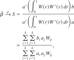
where W = (W1,…,Wk)′ is a k-dimensional vector of independent standard Brownian processes, where

and where

denotes convergence in distribution of the associated probability measures as T → ∞.
Proof. See Park and Phillips (1988, 1989).
Theorem 1 states that when the number of cross-sectional units n is finite, the aggregate relationship may not cointegrate. When n → ∞, this is no longer the case. Under cross-sectional independence, the aggregate relationship cointegrates. Moreover, the asymptotic behavior of the OLS estimator considered here,

, has the same probability limit as the pooled OLS estimator

in Phillips and Moon (1999), defined as

This is stated in the following proposition.
PROPOSITION 1. Assume that

and let

. Then, under cross-sectional independence, when T → ∞ and n → ∞,

and

Proof. See the Appendix.
Note that, following the conclusions of Phillips and Moon (1999), and Sun (2004) under milder conditions, when (n,T) → ∞ sequentially or jointly, we have that

at the rate n if cointegration between yt and xt holds and at the rate

if cointegration between yt and xt fails to hold. Thus,

converges to the average slope coefficient of the individual relationships, irrespective of whether yt and xt cointegrate.
3. PERFECT COINTEGRATION VERSUS SPURIOUS REGRESSION
Theorem 1 describes the properties of the estimator

in the presence of one or more common stochastic trends. If the xit's are driven by a single stochastic trend, k = 1, the limiting distribution of

is

In the presence of a single trend, therefore, the aggregate relationship cointegrates. The OLS estimator

converges to a weighted average of βi coefficients where weights are given by the αi1 coefficients. This finding is consistent with the analysis of Gonzalo (1993). Hall, Lazarová, and Urga (1999) highlight this case when providing a counterexample to the general statement of Pesaran and Smith (1995) that the aggregate relationship does not cointegrate even if all individual units do cointegrate.
When there is more than one common stochastic trend among the right-hand-side variables, k > 1, the aggregate regression is generally spurious, and the estimator

converges in distribution to a nondegenerate random variable. The form of the limiting random variable S in Theorem 1 implies that cointegration occurs only if there exists a constant c such that aj(bi − cai) = 0 for every i and j. This condition is satisfied if and only if either

or

If (9) holds, the aggregate series xt does not have a unit root. We exclude this situation by assumption. If (10) holds, either βi's must be homogeneous, βj = c for all j, or, letting ι = (1,…,1) be an n-dimensional vector of ones, the vector τ − cι, where τ = (β1,β2,…, βn)′, needs to be orthogonal to each of the columns of the matrix A. Formally, this could be represented as

This can occur only if the vector τ − cι lies in the space spanned by the columns of matrix A. Although this is true when k = 1, it does not necessarily hold when k > 1.
Condition (11), characterizing the cases under which the aggregate system cointegrates, has been derived from the limiting distribution of S in Theorem 1. One could also arrive at this condition from population regression. This alternative derivation of equation (11) is reported in the Appendix.
If there is more than one trend driving the regressors and neither of conditions (9) and (10) is satisfied, the aggregate relationship does not cointegrate. This qualifies the regression as spurious. However, the dispersion of the limiting variable depends on the parameters of the underlying processes; therefore for some values of parameters the distribution can be nearly degenerate. In such a case, the estimator

, though inconsistent, may not be entirely worthless. It is therefore of some interest to analyze factors on which the variance of the limiting distribution depends.
Theorem 1 indicates that when k > 1, the limiting distribution of

is S = (∫WaWb)/(∫Wa2), where the scalars Wa and Wb are Brownian processes defined as a′W and b′W, where W is a standard Brownian process. The process Wb can be decomposed as

where Wc is a Brownian process independent of Wa. The variance of Wc is var Wc(r) = (b′b − (a′b)2/a′a)r. It follows that

where

stands for equality in distribution,

and B1, B2 are independent standard Brownian processes. The first two moments of S are

and

If cointegration occurs, S degenerates to a constant value of a′b/a′a. When cointegration fails to occur, the dispersion of S around a′b/a′a is nonzero. The variance of S can thus be used as a measure of the distance from the case of aggregate cointegration.1
We thank an anonymous referee for suggesting this decomposition of the limiting distribution of S.
Now let

Given that equations (6) and (7) are cointegration relationships, it is straightforward to see that LRV(Δyt) = b′b and LRV(Δxt) = a′a. Therefore, from (13) we obtain

where sin(a,b) denotes the sine of the angle between vectors a and b. Decomposition (14) motivates the construction of a measure of the departure from cointegration. To obtain a scale-invariant statistic, we normalize the variance of S and define

Further,

where cos(a,b) and tan(a,b) denote the cosine and tangent of the angle between vectors a and b, respectively.
It is evident that d only depends on the angle between the two vectors a and b. The smaller the angle between the two vectors, the closer we are to the case of aggregate cointegration, which occurs when d = 0.
The definition (15) is based on the variance of the random variable S and the notion of superconsistency when cointegration is present. Alternatively, d may be derived as a measure of the degree of noncointegration directly from equation (11). This latter derivation, suggested by a referee, is reported in the Appendix.
In general, the parameters a, b are unknown. A feasible version

of the statistic d can be computed using estimates

and

of a and b as

We now explore the asymptotic properties of the estimator

. When the aggregate relationship cointegrates, var S = 0, and equation (13) implies that (a′b)2 = (a′a)(b′b). By the Schwarz inequality, the last equality holds if and only if there exists a constant C such that b = Ca. Because a′b/a′a = C, the aggregate relationship cointegrates if and only if b = (a′b/a′a)a. To model the system under no aggregate cointegration, we consider local departures from cointegration of the form

where δT′ a = 0 and TδT → δ as T → ∞. In this formulation, when δ = 0, the aggregate regression cointegrates, whereas when δ ≠ 0, aggregate cointegration fails to occur. The following theorem characterizes the rate of convergence of

.
THEOREM 2. Let

and

be superconsistent estimators of a and b, i.e.,

and

. Under the local departure from cointegration (16) with δ = 0 (cointegration) or δ ≠ 0 (no cointegration),

Proof. See the Appendix.
The rate of convergence of

is of order T−2. When the stochastic trends zt's are observable, consistent estimators of a and b can be obtained via ordinary least squares (OLS) by regressing xt and yt on zt, respectively. Such estimates are superconsistent because, irrespective of the existence of a cointegration relationship between xt and yt, xt and yt always cointegrate with zt by assumption. When zt's are unobservable, superconsistent estimators of a and b can be obtained by estimating OLS regressions of xt and yt on estimated trends

, as long as

's estimate zt's consistently. A procedure for estimating zt has been proposed by Kao, Trapani, and Urga (2005).
The following theorem gives the limiting distribution of

when the zt's are observable.
THEOREM 3. Let

where dB(r) = (a′b/a′a)dWu(r) − dWv(r) and Wu and Wv are Brownian processes associated with the partial sums of processes ut and vt in (7) and (6) respectively. Under the local departure from cointegration (16) with δ = 0 (cointegration) or δ ≠ 0 (no cointegration),

Proof. See the Appendix.
Equation (18) shows that the limiting distribution of

is the sum of three terms: the positive constant ∥a∥2∥δ∥2(a′b)−2, the nonzero mean random variable D, and the zero-mean random variable 2∥a∥2(a′b)−2δ′(∫WW′)−1∫WdB. Under no cointegration, when δ = 0, the statistic

has a different asymptotic distribution than under cointegration. This indicates that the statistic

would be a suitable basis to test for the null of aggregate cointegration against local alternatives of aggregate noncointegration.
4. CONCLUSIONS
In nonstationary heterogeneous panels where each unit cointegrates, the aggregate relationship does not cointegrate unless the coefficients describing micro relationships satisfy a set of conditions. In reality these conditions are in general not satisfied, and aggregate cointegration does not hold. Our paper takes a closer look at the conditions for cointegration at the macro level to hold when the conditions for perfect aggregation are violated. The question then is whether the macro relationship is observationally equivalent to a cointegrating equation. We propose a framework for the case of finite n and large T. Our results can be viewed as complementary to those of Phillips and Moon (1999) where the analysis is carried out for the case n → ∞.
We derive an asymptotic measure, d, of the distance from the case of aggregate cointegration. We also propose an estimator

that converges to d at a rate of Op(T−2). We prove that the departure from cointegration depends on the angle between vectors a and b that describe the heterogeneity of the response of yt to xt.
Our paper gives support to the view that even if the conditions for perfect aggregation are violated, the aggregate regression is still useful in characterising the macro relationship.
APPENDIX
Derivation of Equation (11) Using Population Regression.
An alternative way to derive condition (11) is from the population equations. Aggregating at the micro level the data generating process for each yit, namely,

one obtains

for some constant c. Because

is weakly dependent, yt and xt are cointegrated if we assume that the remainder of the error term in equation (A.1),

, cancels out. This will occur if and only if

for all j's. This is the scalar form of equation (11).
Alternative Measure of Departure from Cointegration.
Condition (11) provides an alternative way to understand when perfect cointegration holds. Given that this occurs if and only if

one possible measure of the degree of noncointegration could be obtained by considering the following quantity:

The solution to this minimization problem is given by

and the minimum value attained by the objective function is equal to

Hence, a possible measure of the departure from aggregate cointegration is given by sin2(a,b). This measure is equivalent to definition (15) and has an appealing interpretation. When the βi's are homogeneous across all i's, it is equal to zero by definition; i.e., aggregate cointegration always holds. This holds also under more general conditions, namely, when the vectors a and b are parallel.
Proof of Proposition 1. Consider the OLS estimator

As T → ∞ and n → ∞, we have

proving that

.
As far as the pooled OLS estimator,

, is concerned, we have
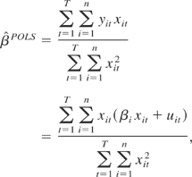
and as T → ∞ and n → ∞, it holds that

proving

. This proves the equivalence of the probability limits of

and

. █
Proof of Theorem 2. Recall that C = a′b/a′a and thus the orthogonal projection of vector b on vector a is (a′b/a′a)a = Ca. In this notation, δT = b − Ca, a′b = C∥a∥2, and ∥b∥2 = C2∥a∥2 + ∥δT∥2 so that ∥b∥ = |C|∥a∥ + O(T−1).
LEMMA 1. Under the local departures from aggregate cointegration,

where sgn(C) is the sign of C and
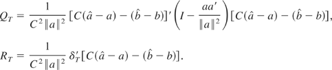
Proof. We have

Superconsistency of

and

implies that

. The Taylor expansion gives us

where

. Similarly for

we have

and

where

. Therefore the denominator of (A.2) is equal to ∥a∥2∥b∥2 + Op(T−2) = C2∥a∥4 + Op(T−2). As far as the numerator of (A.2) is concerned, simple algebra yields

Because εa, εb, and δT are Op(T−1), the last display is equal to

This implies that

Lemma 1 implies that, under the local departures from aggregate cointegration,

. Because

and cos(a,b) = sgn(C)(1 + Op(T−2)), we have

This implies that

because tan2(a,b) = Op(T−2) and QT − 2RT = Op(T−2). █
Proof of Theorem 3. Recall that, by definition, the OLS estimators for a and b in equations (6) and (7) are given by

Therefore

Because both equations (6) and (7) are cointegration relationships, the OLS estimators

and

are superconsistent; i.e., it holds that εa = Op(T−1) and εb = Op(T−1). Let Wv(r) and Wu(r) be the Brownian motions associated with the partial sums of vt and ut, respectively. Then the central limit theorem for functional spaces, implied by Assumptions (a)–(e), ensures that


Under the local departure from cointegration (16) with δ = 0 (cointegration) or δ ≠ 0 (no cointegration) we have that, from equation (A.3),

and because

we have that

Also, as T → ∞

Last, we have that

Combining (A.7), (A.8), and (A.9) we finally get equation (18). █


