1. Introduction
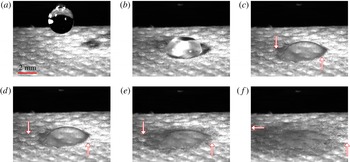
Wetting of permeable substrates by liquids is an important phenomenon in natural and industrial processes such as filtration, printing, textile manufacturing, flow near rocks and dirt and absorption of raindrops by plants (Clarke et al. Reference Clarke, Blake, Carruthers and Woodward2002; Anderson Reference Anderson2005; Arora et al. Reference Arora, Deshpande and Chakravarthy2006; Kumar & Deshpande Reference Kumar and Deshpande2006). The presence of physical or chemical heterogeneities on the substrate may significantly alter liquid spreading and the shape of the liquid interface. This in turn may alter the imbibition of the liquid into the substrate. An example of the influence of surface roughness is shown in figure 1, where a water droplet spreads on a permeable fibre mat. The droplet contact line pins to the surface of the fibre mat, and the droplet elongates toward the lower left corner of the images.
Images of a
 $11.13~{\rm\mu}\text{l}$
water droplet spreading on a 0.214 mm thick polybutylene terephthalate fibre mat at
 $t=0$
s (a),
 $t=0.104$
s (b),
 $t=0.212$
s (c),
 $t=0.312$
s (d),
 $t=0.412$
s (e),
 $t=0.812$
s (f). The arrows indicate the approximate position of the wetting front in the fibre mat.

A common approach to describing the spreading of droplets on permeable substrates is to assume that the droplet–air interface maintains a spherical-cap or parabolic shape (Denesuk et al. Reference Denesuk, Smith, Zelinski, Kreidl and Uhlmann1993; Davis & Hocking Reference Davis and Hocking2000; Clarke et al. Reference Clarke, Blake, Carruthers and Woodward2002; Starov et al. Reference Starov, Kostvintsev, Sobolev, Velarde and Zhdanov2002a ,Reference Starov, Kosvintsev, Sobolev, Velarde and Zhdanov b ; Anderson Reference Anderson2005). While this description works well in some cases for horizontal substrates (Starov et al. Reference Starov, Kostvintsev, Sobolev, Velarde and Zhdanov2002a ; Kumar & Deshpande Reference Kumar and Deshpande2006), it is not appropriate when factors such as substrate inclination, external shear due to an airflow and substrate heterogeneities cause the droplet–air interface to adopt different shapes.
A more versatile approach is to apply lubrication theory to derive an evolution equation for the droplet–air interface. Such models often incorporate a precursor film to model the behaviour of the contact-line region (Alleborn & Raszillier Reference Alleborn and Raszillier2004; Zadražil, Stepanek & Matar Reference Zadražil, Stepanek and Matar2006). However, to prevent the precursor film from being absorbed into the substrate, the substrate permeability is modified in an ad hoc manner by requiring it to be a function of the droplet thickness.
Although spherical-cap and lubrication-theory-based approaches can successfully describe some experimental observations of droplets spreading on horizontal permeable substrates, there are other phenomena they have not been able to explain to date. Kumar & Deshpande (Reference Kumar and Deshpande2006) conducted experiments involving the spreading of silicone oil (SO) and polyvinyl alcohol (PVA)/water solutions on substrates made of glass fibres. Whereas the data for the SO droplets agreed well with predictions of the spherical-cap and lubrication-theory-based approaches, the data for the PVA/water droplets exhibited qualitatively different behaviour. The radius of the PVA/water droplets remained constant for a significant fraction of the total imbibition time, and then decreased rapidly toward the end of the imbibition process. In contrast, the radius of the SO droplets increased initially and then gradually decreased. A regime of constant droplet radius has also been observed in experiments involving the suction of water/glycerol drops through porous membranes (Bacri & Brochard-Wyart Reference Bacri and Brochard-Wyart2000).
The surface tension of PVA/water is more than twice that of SO, which may make it more prone to contact-line pinning when surface roughness is present (Berg Reference Berg2009). However, the spherical-cap and lubrication-theory-based approaches described above do not account for surface roughness, and this may be the reason why they are unable to reproduce the constant-droplet-radius regime.
The objective of the present paper is develop a new lubrication-theory-based model for the spreading of droplets on permeable substrates. Two key features distinguish this new model from those developed previously. First, the new model incorporates surface roughness and so is able to reproduce the constant-droplet-radius regime observed in the experiments of Kumar & Deshpande (Reference Kumar and Deshpande2006). Second, the new model uses a modified boundary condition for liquid imbibition that removes the need to introduce an ad hoc thickness-dependent permeability. The model can be compared against experimental data to extract parameter values such as the effective substrate permeability. Because the model does not assume a fixed interface shape (e.g. spherical cap), it can be used to make predictions of droplet spreading in situations where the interface adopts more complex shapes.
Section 2 of the paper presents the governing equations and the modified boundary condition for liquid imbibition. Section 3 describes how numerical solutions to the model are obtained, as well as important features of these solutions. Comparisons between model predictions and experimental data in the absence of contact-line pinning are presented in § 4. In § 5, surface roughness is incorporated and comparisons are made between the model predictions and the experiments of Kumar & Deshpande (Reference Kumar and Deshpande2006), where contact-line pinning is present. Concluding remarks are offered in § 6.
2. Mathematical model
2.1. Governing equations
We consider an axisymmetric droplet spreading over a horizontal permeable substrate (figure 2
a). The droplet flows with velocity
 $(u,w)$
, which denote the radial
 $(r)$
and vertical
 $(z)$
components of the velocity vector, respectively. The substrate is located at
 $z=0$
, and the
 $z$
-axis coincides with the droplet symmetry axis. The droplet is assumed to be thin, so that its characteristic height
 $h^{\ast }$
and radius
 $l^{\ast }$
satisfy
 ${\it\varepsilon}=h^{\ast }/l^{\ast }\ll 1$
, allowing us to apply lubrication theory.
(a) Schematic of an axisymmetric droplet on a permeable substrate. The diameter of the pores has been greatly exaggerated for illustrative purposes. (b) Cross section of the droplet. This schematic shows a precursor film of height
 $b^{\ast }$
and the pores saturated with liquid.

The characteristic spreading speed of the droplet is
 $u^{\ast }={\it\varepsilon}^{3}{\it\sigma}/3{\it\mu}$
, where
 ${\it\sigma}$
is the surface tension of the liquid and
 ${\it\mu}$
its viscosity. The time scale is defined by
 $t^{\ast }=l^{\ast }/u^{\ast }$
, the pressure scale by
 $p^{\ast }=h^{\ast }{\it\sigma}/{l^{\ast }}^{2}$
and the disjoining-pressure scale by
 $\mathscr{A}^{\ast }=p^{\ast }$
. With these scales we define the following dimensionless variables (denoted with primes):
 $$\begin{eqnarray}\left.\begin{array}{@{}c@{}}\displaystyle r=l^{\ast }r^{\prime },\quad z=h^{\ast }z^{\prime },\quad u=u^{\ast }u^{\prime },\quad w={\it\varepsilon}u^{\ast }w^{\prime }\\ t={\displaystyle \frac{l^{\ast }}{u^{\ast }}}t^{\prime },\quad p=p^{\ast }p^{\prime },\quad {\it\Pi}=\mathscr{A}^{\ast }{\it\Pi}^{\prime },\end{array}\right\}\end{eqnarray}$$
where
 ${\it\Pi}$
is the disjoining pressure.
At leading order, the equations governing momentum and mass conservation are
 $$\begin{eqnarray}\displaystyle & \displaystyle 0=-3p_{r^{\prime }}^{\prime }+u_{z^{\prime }z^{\prime }}^{\prime }, & \displaystyle\end{eqnarray}$$
 $$\begin{eqnarray}\displaystyle & \displaystyle 0=-p_{z^{\prime }}^{\prime }-B, & \displaystyle\end{eqnarray}$$
 $$\begin{eqnarray}\displaystyle & \displaystyle w_{z^{\prime }}^{\prime }+\frac{1}{r^{\prime }}\frac{\partial }{\partial r^{\prime }}(r^{\prime }u^{\prime })=0, & \displaystyle\end{eqnarray}$$
 $B={l^{\ast }}^{2}{\it\rho}g/{\it\sigma}$
is the Bond number,
 ${\it\rho}$
is the density of the liquid and
 $g$
is the magnitude of the gravitational acceleration. The droplet–air interface is defined by
 $z^{\prime }=h^{\prime }(r^{\prime },t^{\prime })$
, and the kinematic condition there is
 $$\begin{eqnarray}h_{t^{\prime }}^{\prime }=w^{\prime }-u^{\prime }h_{r^{\prime }}^{\prime }.\end{eqnarray}$$
The normal and tangential components of the interfacial stress balance are, at leading order,
 $$\begin{eqnarray}\displaystyle & \displaystyle p^{\prime }=-\left(h_{r^{\prime }r^{\prime }}^{\prime }+\frac{1}{r^{\prime }}h_{r^{\prime }}^{\prime }\right)-{\it\Pi}^{\prime }, & \displaystyle\end{eqnarray}$$
 $$\begin{eqnarray}\displaystyle & \displaystyle u_{z^{\prime }}^{\prime }=0. & \displaystyle\end{eqnarray}$$
Although the concepts of precursor film and disjoining pressure were originally developed in the context of isothermal liquid spreading on flat impermeable substrates (Schwartz Reference Schwartz1998; Schwartz & Eley Reference Schwartz and Eley1998), they are also helpful in describing more complex situations such as spreading on heated substrates (see Sodtke, Ajaev & Stephan (Reference Sodtke, Ajaev and Stephan2008) and Espín & Kumar (Reference Espín and Kumar2014) and references therein), spreading on substrates with topography (Savva & Kalliadasis Reference Savva and Kalliadasis2011) and spreading on permeable substrates (Alleborn & Raszillier Reference Alleborn and Raszillier2004; Zadražil et al.
Reference Zadražil, Stepanek and Matar2006). To model the behaviour of the droplet contact-line region, we use a precursor film of thickness
 $b^{\ast }=h^{\ast }b^{\prime }$
, and a two-term disjoining pressure
 ${\it\Pi}^{\prime }$
of the form
 $$\begin{eqnarray}{\it\Pi}^{\prime }=\mathscr{A}\left[\left(\frac{b^{\prime }}{h^{\prime }}\right)^{n}-\left(\frac{b^{\prime }}{h^{\prime }}\right)^{m}\right],\end{eqnarray}$$
with the parameter
 $\mathscr{A}\geqslant 0$
and constants
 $n>m>1$
. As previous studies do (Alleborn & Raszillier Reference Alleborn and Raszillier2004; Zadražil et al.
Reference Zadražil, Stepanek and Matar2006), we choose the powers
 $n=3$
and
 $m=2$
because they provide an adequate description of the behaviour of the contact-line region at a reasonable computational cost.
The interaction of the repulsive (first) and attractive (second) terms of (2.8) determine the value of the equilibrium contact angle
 ${\it\theta}_{e}$
(Schwartz Reference Schwartz1998; Schwartz & Eley Reference Schwartz and Eley1998). In addition, we can define an apparent contact angle,
 ${\it\theta}_{a}$
, as the angle between the substrate and the tangent to the point on the interface having the largest slope (Schwartz Reference Schwartz1998; Schwartz & Eley Reference Schwartz and Eley1998). If
 ${\it\theta}_{a}>{\it\theta}_{e}$
, the droplet will spread until
 ${\it\theta}_{a}={\it\theta}_{e}$
. If
 ${\it\theta}_{a}<{\it\theta}_{e}$
, the droplet will retract until
 ${\it\theta}_{a}={\it\theta}_{e}$
. The parameter
 $\mathscr{A}$
and constants
 $n$
and
 $m$
characterize the intermolecular interactions of a given liquid–substrate system (Ruckenstein & Jain Reference Ruckenstein and Jain1974; de Gennes Reference de Gennes1985; Teletzke, Davis & Scriven Reference Teletzke, Davis and Scriven1987; Savva & Kalliadasis Reference Savva and Kalliadasis2011). In addition,
 $\mathscr{A}$
can be related to the value of
 ${\it\theta}_{e}$
(Schwartz Reference Schwartz1998; Schwartz & Eley Reference Schwartz and Eley1998),
 $$\begin{eqnarray}{\it\theta}_{e}\approx {\it\varepsilon}\sqrt{\frac{2(n-m)b\mathscr{A}}{(n-1)(m-1)}}.\end{eqnarray}$$
2.2. Liquid imbibition
Our description of liquid imbibition involves a slight but important modification of the boundary condition used by Davis & Hocking (Reference Davis and Hocking1999). Davis & Hocking (Reference Davis and Hocking1999) consider a substrate with unconnected vertical pores (figure 2 b). Poiseuille flow in each pore driven by excess liquid pressure above the substrate is assumed, with entrance and exit effects neglected. These assumptions give rise to the following boundary condition at the liquid–substrate interface:
 $$\begin{eqnarray}w(r,z=0,t)=-\frac{\hat{{\it\kappa}}}{{\it\mu}}p(r,z=0,t),\end{eqnarray}$$
where
 $\hat{{\it\kappa}}$
is a proportionality constant with units of length. In the case of a substrate with unconnected vertical pores,
 $\hat{{\it\kappa}}$
can be expressed in terms of the pore diameter, number of pores per unit area and substrate thickness (Davis & Hocking Reference Davis and Hocking1999).
Davis & Hocking (Reference Davis and Hocking1999) considered imbibition of a droplet with a fixed contact angle on a permeable substrate. A no-slip condition is used, but it does not give rise to a stress singularity at the contact line since liquid can enter the substrate. As a consequence, the droplet can retract as liquid enters the substrate. However, since there is no contact-line slip or precursor film, the use of the no-slip condition means that the droplet is unable to spread.
Although the no-slip condition could be relaxed by applying a slip law, numerical solutions of the resulting equations are considerably more difficult to obtain than those for a precursor-film model because the contact-line location must be determined along with the droplet height (Savva & Kalliadasis Reference Savva and Kalliadasis2009). For this reason, we are motivated to develop a model that uses a precursor film to describe the contact-line region. However, application of boundary condition (2.10) would cause the precursor film to become absorbed when gravity is present, and the amount of absorption would depend on the relative values of
 $\mathscr{A}$
and
 $B$
. Since comparisons between different values of
 $B$
and
 $\mathscr{A}$
(or
 ${\it\theta}_{e}$
) at fixed precursor-film thickness are desired, such absorption complicates interpretation of the results.
To overcome this limitation, we alter (2.10) so that the thickness of the substrate
 $d^{\ast }$
and the presence of a precursor film above the substrate are taken into account:
 $$\begin{eqnarray}w(r,z=0,t)=-\frac{{\it\kappa}^{\ast }}{{\it\mu}d^{\ast }}p(r,z=b^{\ast },t).\end{eqnarray}$$
The modified condition (2.11) assumes that the flow entering the permeable substrate is driven by the excess liquid pressure above the precursor film (figure 2(b)). The modified boundary condition (2.11) decouples the dynamics of liquid on the substrate from that of liquid in the substrate, and assumes that liquid absorption can be characterized with the coefficient
 ${\it\kappa}^{\ast }$
, which is the effective permeability of the substrate (typically
 $b^{\ast }\ll d^{\ast }$
, so
 $p(r,z=b^{\ast },t)/d^{\ast }$
approximates the pressure gradient across the substrate). This modified condition is appropriate for situations where
 ${\it\rho}gb^{\ast }$
is much less than the pressure in the air, which is usually the case in practice (Popescu et al.
Reference Popescu, Oshanin, Dietrich and Cazabat2012), and it removes the need to introduce a thickness-dependent permeability (Alleborn & Raszillier Reference Alleborn and Raszillier2004; Zadražil et al.
Reference Zadražil, Stepanek and Matar2006).
The simple form of boundary condition (2.10) assumes that the region of the substrate where the condition is applied is completely saturated with liquid (Davis & Hocking Reference Davis and Hocking1999). Experimental studies show that this assumption can readily be met. It has been observed that when droplets are deposited on thin permeable membranes, the spreading and retraction of the droplets occur over regions of the substrate already saturated with liquid, after a brief initial stage where inertial effects are important (Starov et al. Reference Starov, Kostvintsev, Sobolev, Velarde and Zhdanov2002a ; Arora et al. Reference Arora, Deshpande and Chakravarthy2006). This happens because during this initial inertial stage, a wetting front forms in the substrate and immediately below the droplet, and this front quickly spreads ahead of the droplet contact line. This behaviour has been measured experimentally (Starov et al. Reference Starov, Kostvintsev, Sobolev, Velarde and Zhdanov2002a ; Arora et al. Reference Arora, Deshpande and Chakravarthy2006), and is also evident in the images of figure 1, where arrows indicate the approximate position of the wetting front. We note that, in principle, the model developed here could be coupled to a model for the imbibition front in the permeable substrate, similar to previous work (Starov et al. Reference Starov, Kostvintsev, Sobolev, Velarde and Zhdanov2002a ; Alleborn & Raszillier Reference Alleborn and Raszillier2004; Zadražil et al. Reference Zadražil, Stepanek and Matar2006).
To close the system of equations and boundary conditions we follow previous related studies (Davis & Hocking Reference Davis and Hocking1999; Alleborn & Raszillier Reference Alleborn and Raszillier2004; Zadražil et al. Reference Zadražil, Stepanek and Matar2006; Spannuth et al. Reference Spannuth, Neufeld, Wettlaufer and Worster2009) and apply a no-slip condition at the substrate,
 $$\begin{eqnarray}u(r,z=0,t)=0.\end{eqnarray}$$
Although we apply a no-slip condition here, we note that a slip boundary condition for permeable substrates may be needed in some cases (Beavers & Joseph Reference Beavers and Joseph1967; Spannuth et al. Reference Spannuth, Neufeld, Wettlaufer and Worster2009; Talbott et al. Reference Talbott, Xu, Anderson and Seshaiyer2015).
3. Evolution equation
3.1. Solution method
A single evolution equation for the droplet height is obtained by integrating equations (2.2)–(2.4) with respect to
 $z$
, and using boundary conditions (2.5)–(2.7) as well as the dimensionless version of conditions (2.11)–(2.12). The evolution equation is (primes dropped):
 $$\begin{eqnarray}h_{t}=\frac{1}{r}\partial _{r}\left\{rh^{3}\partial _{r}\left(Bh-\mathscr{A}{\it\Pi}-h_{rr}-\frac{1}{r}h_{r}\right)\right\}-{\it\kappa}\left(B(h-b)-\mathscr{A}{\it\Pi}-h_{rr}-\frac{1}{r}h_{r}\right),\end{eqnarray}$$
where the dimensionless imbibition coefficient is
 ${\it\kappa}=3{\it\kappa}^{\ast }{l^{\ast }}^{2}/d^{\ast }{h^{\ast }}^{3}$
.
Equation (3.1) is solved numerically on the domain
 $0\leqslant r\leqslant L$
subject to the boundary conditions
 $$\begin{eqnarray}\left.\begin{array}{@{}c@{}}h_{r}(0,t)=0,\quad h(L,t)=b,\\ h_{rrr}(0,t)=0,\quad h_{r}(L,t)=0.\end{array}\right\}\end{eqnarray}$$
The initial condition is given by a fourth-order polynomial that satisfies conditions (3.2) imposed at
 $r=r_{0}<L$
, and the condition that the volume between
 $r=0$
and
 $r=r_{0}$
is
 $V_{0}+{\rm\pi}b$
, where
 $V_{0}$
is the dimensionless initial droplet volume. The correction
 ${\rm\pi}b$
is the dimensionless volume of the precursor film on a circular region with radius
 $l^{\ast }$
. When making comparisons to experimental data, values of the initial volume and radius are determined from the data and used to set the values of
 $V_{0}$
and
 $r_{0}$
in the calculations. For calculations where we do not compare with experimental data, we set
 $r_{0}=1$
and
 $V_{0}=2$
. Typical values of
 $L$
range from 2 to 5 and typical discretization sizes vary between 500 and 1000 points per unit length.
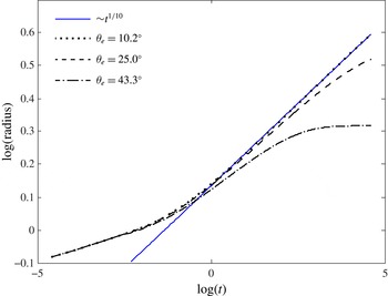
Calculations of droplet radius as a function of time for increasing values of the equilibrium contact angle. The parameters used in these calculations are
 $V_{0}=2$
,
 $L=5$
,
 ${\it\kappa}=0$
,
 $B=0$
and
 $b=10^{-3}$
. The values
 $\mathscr{A}=40,250$
and 1000 correspond to increasing values of
 ${\it\theta}_{e}$
. The solid straight blue line has a slope of
 $1/10$
.

Numerical solutions of (3.1) and (3.2) are obtained with a fully implicit finite-difference scheme. All spatial derivatives are approximated with second-order centred differences and time integration is performed with the DDASPK iterative solver (Brown et al.
Reference Brown, Hindmarsh and Petzold1994). The value of the apparent contact angle is obtained by finding the maximum slope of the interface (Schwartz Reference Schwartz1998; Schwartz & Eley Reference Schwartz and Eley1998) and the position of the apparent contact line is found by extrapolation of the corresponding tangent to the substrate. The radius of the droplet is defined as the distance from the apparent contact line to the
 $z$
-axis. Because the horizontal and vertical coordinates are scaled differently, the value of the apparent contact angle is larger than the value that would be obtained if dimensional values of the coordinates are used. The latter angle can be obtained by multiplying the former angle by
 ${\it\varepsilon}$
.
3.2. Solution features
We now discuss some important features of the numerical solutions to the evolution equation. The case
 ${\it\kappa}=\mathscr{A}=0$
corresponds to a droplet of a perfectly wetting liquid spreading over an impermeable substrate. Lubrication theory predicts that the droplet contact line spreads with speed
 ${\sim}t^{1/10}$
and its height decreases as
 ${\sim}t^{-1/5}$
(Tanner Reference Tanner1979; Oron et al.
Reference Oron, Davis and Bankoff1997). Numerical solutions of (3.1) and (3.2) reproduce this behaviour (comparisons not shown for brevity).
Spreading droplets of partially wetting liquids follow the same power laws as those for perfectly wetting liquids, except when the apparent contact angle approaches the equilibrium angle
 ${\it\theta}_{e}$
(Zosel Reference Zosel1993; Schwartz & Eley Reference Schwartz and Eley1998). This behaviour can be observed in figure 3, where we show the time evolution of the radius of droplets with different values of
 ${\it\theta}_{e}$
. These values of
 ${\it\theta}_{e}$
are not calculated from the approximate formula (2.9); they are the apparent contact angles obtained from calculations for much longer times than those shown in figure 3, when the drop is close to reaching equilibrium.
For small values of
 ${\it\theta}_{e}$
, the curves in figure 3 fall onto the straight blue line with slope
 $1/10$
during the time interval shown. However, as
 ${\it\theta}_{e}$
increases, a deviation from the power-law behaviour is clearly visible. For
 ${\it\theta}_{e}=43.3^{\circ }$
, spreading slows toward the end of the calculation as the droplet approaches an equilibrium state. Figure 3 also shows that the equilibrium state is approached more quickly as
 ${\it\theta}_{e}$
increases.
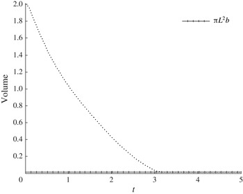
When the effective permeability
 ${\it\kappa}$
is positive, liquid imbibition leads to a continuous decrease in droplet volume (mass), as illustrated in figure 4. Before the droplet disappears, the volume of the droplet decreases monotonically until the volume reaches that of a uniform disk of height
 $b$
and radius
 $L$
, where
 $L$
is the size of the computational domain. At this point the solution has reduced to a precursor film,
 $h(r,t)=b$
, and it will remain unchanged for the rest of the calculation (figure 4). Thus, we define the imbibition time
 $t_{d}$
as the time when the volume of the computed solution equals
 ${\rm\pi}L^{2}b$
, and we also use this definition as a stopping criterion for the calculations. This observation also suggests that the exact solution of (3.1)–(3.2),
 $h(r,t)\equiv b$
, is a stable solution.
Calculation of droplet volume as a function of time for the case
 $V_{0}=2$
,
 $L=5$
,
 ${\it\kappa}=0.1$
,
 $B=0$
,
 $b=10^{-3}$
and
 ${\it\theta}_{e}=43.3^{\circ }$
(
 $\mathscr{A}=1000$
). The line marked with crosses indicates the volume of a uniform disk of height
 $b=10^{-3}$
and radius
 $L=5$
.

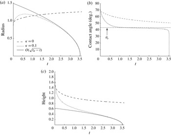
In figure 5 we show the evolution of the radius, apparent contact angle and height corresponding to the calculation of figure 4 and for the case of an impermeable substrate. Initially, the droplet on the permeable substrate spreads until a maximum radius is reached (figure 5
a). Since liquid is continuously imbibed by the substrate, the contact line then starts to retract until the droplet disappears at time
 $t_{d}=3.53$
. The maximum radius is reached as the apparent contact angle approaches its equilibrium value (figure 5
b). During contact-line retraction, and just before the droplet is completely imbibed, the apparent contact angle stays close to the equilibrium angle, decreasing in value slightly and slowly. This indicates that during retraction, the shape of the droplet–air interface near the contact line varies little as well.
Evolution of the (a) droplet radius, (b) apparent contact angle and (c) droplet height at
 $r=0$
for the case
 $V_{0}=2$
,
 $L=5$
,
 $B=0$
,
 $b=10^{-3}$
and
 ${\it\theta}_{e}=43.3^{\circ }$
(
 $\mathscr{A}=1000$
) for a droplet spreading on permeable (
 ${\it\kappa}=0.1$
) and impermeable (
 ${\it\kappa}=0$
) substrates. Dotted and dashed lines indicate the numerical solutions, and the solid lines in (a) and (c) are obtained from the self-similar solution described in appendix A (the solution is valid close to the end of imbibition). In (b), the dashed-dot line indicates the equilibrium contact angle.

For the impermeable substrate, the droplet spreads until an equilibrium state is reached and no retraction occurs. Figure 5(b) shows that the apparent contact angle for a droplet on a permeable substrate approaches the equilibrium value much faster compared to a droplet on an impermeable substrate. Figure 5(c) shows that the height at the droplet centre decreases more rapidly for the permeable substrate, which is consistent with the faster approach to the equilibrium contact angle.
For times close to the end of imbibition, a self-similar solution to (3.1) can be obtained (see appendix A). This solution predicts that both the droplet radius and height
 ${\sim}\sqrt{t_{d}-t}$
, and the numerical solution shown in figure 5(a,c) is in good agreement with this prediction.
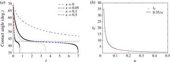
In figure 6(a), we show the time evolution of the apparent contact angle for different values of
 ${\it\kappa}$
. As
 ${\it\kappa}$
increases, the imbibition time decreases. As a consequence, the contact angle decreases more rapidly and stays closer to its equilibrium value for a shorter time. Figure 6(b) shows that the imbibition time is proportional to
 $1/{\it\kappa}$
.
(a) Evolution of the apparent contact angle for droplets spreading on substrates with different effective permeability values
 ${\it\kappa}$
. (b) Imbibition time
 $t_{d}$
as function of
 ${\it\kappa}$
. The crosses represent calculated values and the continuous line indicates that
 $t_{d}\sim 1/{\it\kappa}$
. Values of the other parameters are
 $V_{0}=2$
,
 $L=5$
,
 $B=0$
,
 $b=10^{-3}$
and
 ${\it\theta}_{e}=43.3^{\circ }$
(
 $\mathscr{A}=1000$
).

Finally, we summarize the results of several parametric studies we have performed. Decreasing the equilibrium contact angle results in a larger maximum spreading radius, a longer plateau in the apparent contact angle and a longer imbibition time. The longer imbibition time results because the interfacial curvature drives the imbibition, and this curvature decreases as the equilibrium contact angle does. Increasing the initial volume of the droplet has the same effect as decreasing the equilibrium contact angle. Increasing the Bond number shortens the imbibition time and the plateau length in the apparent contact angle due to the stronger driving force for imbibition. The maximum spreading radius does not change significantly for an
 $O(1)$
change in
 $B$
.
4. Comparison of model predictions with experimental data in absence of contact-line pinning
In this section, we make comparisons between the model predictions and previously published experimental data in cases where contact-line pinning is absent. To do so, we use experimental values of the maximum radius as the characteristic radius
 $l^{\ast }$
, and the corresponding droplet height as the characteristic height
 $h^{\ast }$
. If measurements of the droplet height are not given, we use measurements of the volume or apparent contact angle and a spherical-cap approximation to obtain a characteristic height. Since the maximum radius is attained when the apparent contact angle approaches its equilibrium value (figure 5), these choices of characteristic length scales correspond to the height and radius when the apparent contact angle is close to its equilibrium value. For the solution of (3.1)–(3.2), we use
 $L=2$
.
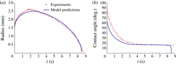
In figure 7, we show comparisons for the radius and apparent contact angle of a SO droplet spreading on a glass fibre mat (Kumar & Deshpande Reference Kumar and Deshpande2006). The model predictions match well the retraction of the contact line and the corresponding evolution of the contact angle. The agreement is not as good for
 $t\lesssim 2$
s, because no effort was made to have a more accurate initial condition. Indeed, the initial measured contact angle is close to
 $90^{\circ }$
, which means that the initial shape of the droplet in the experiment is close to a hemisphere, and so does not satisfy the small-slope restriction of lubrication theory.
Experimental measurements (symbols) and model predictions (lines) of the (a) radius and (b) apparent contact angle for a SO droplet spreading on a 1.12 mm thick glass fibre mat (case corresponding to figure 3 of Kumar & Deshpande Reference Kumar and Deshpande2006). Parameters obtained from the experimental data are
 $V_{0}^{\ast }=9.18~{\rm\mu}\text{l}$
,
 $l^{\ast }=2.61$
mm,
 $h^{\ast }=0.72$
mm and
 $B=3.31$
. Parameters that give the best fit of the model predictions to the experimental data are
 $\mathscr{A}=1.44/b$
(
 ${\it\theta}_{e}=16.7^{\circ }$
),
 $b=10^{-3}$
and
 ${\it\kappa}^{\ast }=5.33\times 10^{-4}~\text{cm}^{2}$
.

The parameters used to match the model predictions to the experimental data are the effective permeability
 ${\it\kappa}$
, which is obtained by matching the imbibition time to
 $t_{d}$
, and the disjoining-pressure parameter
 $\mathscr{A}$
, which is obtained by matching the apparent contact angle during droplet retraction (in doing this, we account for the different values of the angle that are obtained when using our scaled variables versus dimensional variables (§ 3.1)). Typically,
 ${\it\kappa}$
is varied first to match
 $t_{d}$
, then the values of
 ${\it\kappa}$
and
 $\mathscr{A}$
are varied together until good agreement is found.
In general, the value of the precursor-film thickness
 $b$
would be obtained by matching the model predictions to the experimental spreading speed. However, spreading occurs over a relatively short time period due to liquid absorption, and we found that matching
 $b$
was typically not necessary because good agreement was often obtained with
 $b=10^{-3}$
. This value was initially chosen for its consistency with the values
 $b=5\times 10^{-3}$
and
 $b=5\times 10^{-4}$
used by Schwartz & Eley (Reference Schwartz and Eley1998), which produce good agreement for water droplets spreading on (impermeable) glass (Teletzke et al.
Reference Teletzke, Davis and Scriven1987; Schwartz & Eley Reference Schwartz and Eley1998). A similar observation regarding the value of
 $b$
was reported also by Alleborn & Raszillier (Reference Alleborn and Raszillier2004) in their study of liquid spreading on permeable substrates.
The dimensional thickness of the precursor film is
 ${\sim}720$
nm, which is within the range of values that have been reported in the literature (
 ${\sim}10$
nm to
 ${\sim}1~{\rm\mu}\text{m}$
(Popescu et al.
Reference Popescu, Oshanin, Dietrich and Cazabat2012)). The value of the disjoining-pressure parameter that we obtain following the procedure described above is
 $\mathscr{A}=1.44/b$
, which is consistent with the values used in other computational studies that use a two-term disjoining pressure model (
 $\mathscr{A}=4/b$
, for example Schwartz, Roux & Cooper-White (Reference Schwartz, Roux and Cooper-White2005)).
We note that making a meaningful comparison between experimentally measured values of the effective permeability and model predictions is difficult due to the model’s simplified description of the pore structure in the permeable substrate (Spannuth et al.
Reference Spannuth, Neufeld, Wettlaufer and Worster2009). In addition, measured values of the effective permeability can vary by several orders of magnitude depending on the liquid/substrate system. For example, Bacri & Brochard-Wyart (Reference Bacri and Brochard-Wyart2000) report permeability values of
 ${\sim}10^{-11}~\text{cm}^{2}$
(water/glycerol through membranes), and Spannuth et al. (Reference Spannuth, Neufeld, Wettlaufer and Worster2009) report permeability values of
 ${\sim}10^{-3}~\text{cm}^{2}$
(syrup through a bed of vertically oriented drinking straws). For the calculations shown in figure 7, we obtain an effective permeability of
 ${\it\kappa}^{\ast }=5.33\times 10^{-4}~\text{cm}^{2}$
, which falls within this range. Measurements of the effective permeability were not reported in Kumar & Deshpande (Reference Kumar and Deshpande2006).
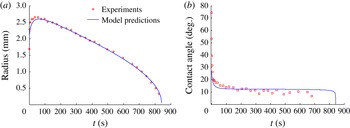
As a further test of the model, we show in figure 8 a comparison between model predictions and experimental data extracted from Starov et al. (Reference Starov, Kostvintsev, Sobolev, Velarde and Zhdanov2002a
) for a SO droplet spreading on a cellulose nitrate membrane filter. The imbibition process here is much slower than that presented in figure 7, and as in that case, the model predictions agree well with the experimental data after a brief initial period because of the large values of the apparent contact angle at the start of the experiment. As before, the value of
 $\mathscr{A}$
used here is consistent with that used in prior models, and the value of
 ${\it\kappa}^{\ast }$
obtained from the model is consistent with prior experimental measurements (measurements of the effective permeability were not reported in Starov et al. (Reference Starov, Kostvintsev, Sobolev, Velarde and Zhdanov2002a
)).
Experimental measurements (symbols) and model predictions (lines) of the (a) radius and (b) apparent contact angle for a SO droplet spreading on a 0.13 mm thick cellulose nitrate membrane filter (case corresponding to SO500 oil and membrane with pore size 3
 ${\rm\mu}\text{m}$
in figures 6 and 7 of Starov et al. (Reference Starov, Kostvintsev, Sobolev, Velarde and Zhdanov2002a
)). Parameters obtained from the experimental data are
 $V_{0}^{\ast }=6.85~{\rm\mu}\text{l}$
,
 $l^{\ast }=2.66$
mm,
 $h^{\ast }=0.37$
mm and
 $B=3.18$
. Parameters that give the best fit of the model predictions to the experimental data are
 $\mathscr{A}=2.9/b$
(
 ${\it\theta}_{e}=12.3^{\circ }$
),
 $b=10^{-3}$
and
 ${\it\kappa}^{\ast }=4.55\times 10^{-8}~\text{cm}^{2}$
.

The results of this section show that the model predictions agree well with experimental data for droplets spreading on horizontal permeable substrates in the absence of contact-line pinning. The values of the model parameters (
 ${\it\kappa}^{\ast }$
,
 $\mathscr{A}$
,
 $b^{\ast }$
) used for these comparisons are consistent with those in other experimental and theoretical studies. These parameters are essentially material parameters and would not be expected to change significantly in other flow configurations. Thus, the model may also give good predictions if it is modified to account for more complicated situations such as droplets sliding down inclined planes or droplets subject to an external air flow, which are beyond the reach of spherical-cap models.
5. Surface roughness and contact-line pinning
In this section, we discuss how the model described above can be modified to describe contact-line pinning due to surface roughness. As we will see, this modification enables the model to describe experimental observations that cannot be captured by spherical-cap models.
5.1. Evolution equation
To describe surface roughness we introduce a shape function,
 $z={\it\eta}(r)$
, which gives the position of the substrate–liquid interface. To be consistent with lubrication theory, and in order to be able to properly define a contact angle,
 ${\it\eta}$
is required to be smooth and to satisfy
 ${\it\eta}_{r}=O(1)$
(Savva & Kalliadasis Reference Savva and Kalliadasis2009). (Note that since
 ${\it\eta}$
and
 $r$
have been made dimensionless using different scales,
 ${\it\eta}_{r}=O(1)$
corresponds to
 ${\it\eta}_{r^{\ast }}^{\ast }=O({\it\epsilon})$
, where the quantities with the star superscript are dimensional.) For computational reasons, we also require
 ${\it\eta}$
to vary on length scales larger than the precursor-film thickness
 $b$
. Under the assumption of
 ${\it\eta}$
being axisymmetric, we can express the position of the droplet–air interface by
 $$\begin{eqnarray}z=H(r,t)\equiv h(r,t)+{\it\eta}(r).\end{eqnarray}$$
The equations of mass and momentum conservation (2.2)–(2.4) are not affected by the inclusion of the shape function
 ${\it\eta}$
. However, the kinematic condition and interfacial stress balances (2.5)–(2.7) are now applied at
 $z=H(r,t)$
. At the substrate
 $z={\it\eta}$
, we impose the no-slip condition (2.12) and the vertical flow condition (2.11), with the pressure evaluated at
 $z=b+{\it\eta}$
instead of
 $z=b$
(Savva & Kalliadasis Reference Savva and Kalliadasis2009). Following the derivation described in § 3.1 we arrive at the updated evolution equation
 $$\begin{eqnarray}\displaystyle h_{t} & = & \displaystyle \frac{1}{r}\partial _{r}\left\{rh^{3}\partial _{r}\left(B(h+{\it\eta})-(h+{\it\eta})_{rr}-\frac{1}{r}(h+{\it\eta})_{r}-\mathscr{A}{\it\Pi}\right)\right\}\nonumber\\ \displaystyle & & \displaystyle -\,{\it\kappa}\left(B(h-b)-\mathscr{A}{\it\Pi}-(h+{\it\eta})_{rr}-\frac{1}{r}(h+{\it\eta})_{r}\right).\end{eqnarray}$$
The expression for
 ${\it\Pi}$
is the same as (2.8), with
 $h$
now representing the film thickness rather than the film height.
We solve (5.2), subject to conditions (3.2), with the same numerical scheme described in § 3.1. For the shape function, we restrict ourselves to substrates that are flat everywhere except for a defect that takes the form of a Gaussian depression,
 ${\it\eta}(r)=-a\exp (-(r-r_{obs})^{2}/2s_{d}^{2})$
, located at
 $r_{obs}$
with standard deviation
 $s_{d}\sim 10b$
and a comparable height
 $a\sim 10b$
. For simplicity, we also require the shape function
 ${\it\eta}$
to satisfy the conditions
 ${\it\eta}={\it\eta}_{r}=0$
at the edge of the computational domain
 $r=L$
, which is easily satisfied by making
 $L$
large enough (for the calculations here,
 $L=2$
is sufficient). The initial condition is the same as that described in § 3.1.
For substrates that are not flat, the definitions of apparent contact line and apparent contact angle given in § 3.1 have to be modified to account for substrate curvature. This can be done by considering the mesoscopic angle
 ${\it\theta}_{m}$
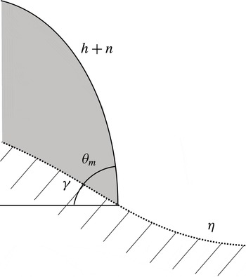
(Savva & Kalliadasis Reference Savva and Kalliadasis2009), which we define as the angle that the droplet–air interface makes with respect to the substrate. Since the droplet and the substrate are axisymmetric, the mesoscopic angle can be determined from the expression (see appendix B for derivation)
 $$\begin{eqnarray}\tan ({\it\theta}_{m})=\frac{h_{r}}{1+(h_{r}+{\it\eta}_{r}){\it\eta}_{r}},\end{eqnarray}$$
and the apparent contact angle
 ${\it\theta}_{a}$
is now obtained by choosing the maximum value of
 ${\it\theta}_{m}$
along the interface. Since the substrate is no longer flat, the position of the apparent contact line
 $r_{cl}$
is found by extrapolating the line tangent to the droplet having slope
 ${\it\theta}_{a}$
onto the substrate. Examples of
 ${\it\theta}_{a}$
,
 ${\it\theta}_{m}$
and the apparent contact line calculated according to these definitions are discussed in § 5.2.
All of the results described in previous sections are recovered when
 ${\it\eta}=0$
or when the defect is located away from the maximum spreading radius of the droplet. We also note that
 $h(r,t)=b$
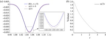
is no longer an exact solution of (5.2) if the substrate is not completely flat, as can easily be checked by substitution. Nevertheless, for non-planar permeable substrates, (5.2) admits a steady-state solution illustrated in figure 9.
(a) Droplet height
 $H(r,t)$
at time
 $t=5$
, near the substrate defect. The defect is located at
 $r_{obs}=1.05$
, and other parameters are
 $V_{0}=2$
,
 $L=2$
,
 ${\it\kappa}=0.1$
,
 $B=0$
,
 $b=10^{-3}$
and
 ${\it\theta}_{e}=43.3^{\circ }$
(
 $\mathscr{A}=1/b$
). The inset shows a magnification of the bottom of the defect, and the crosses mark the curve
 ${\it\eta}(r)+b$
. (b) Time evolution of the droplet volume. The line marked with crosses indicates the volume of a uniform disk of height
 $b=10^{-3}$
and radius
 $L=2$
.

Figure 9(a) shows the droplet–air interface near the defect at a time when the interface height is no longer changing (away from the defect the substrate is flat and
 $h=b$
). Figure 9(b) shows the time evolution of the droplet volume, and after imbibition is completed at time
 $t_{d}=3.18$
, the final height and the volume of the droplet no longer vary. The line marked by crosses in figure 9(b) indicates the volume of a uniform film of thickness
 $b$
. As can be seen in the inset of figure 9(a), the steady-state solution is not quite equal to this; the uniform film has a volume that is approximately 0.999 times the volume of the steady-state solution.
5.2. Contact-line pinning
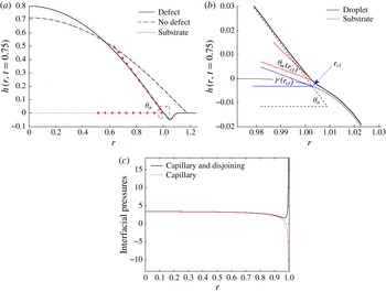
In figure 10(a) we compare the height of a droplet spreading on a permeable substrate that has a defect with the height of an identical droplet spreading on a completely flat substrate. As shown in the figure, the contact line pins to the defect, altering the shape of the interface and increasing the value of the apparent contact angle. We note that this pinning should be interpreted as an apparent pinning since the contact line may still move very slowly.
(a) Interface height
 $h(r,t=0.75)+{\it\eta}(r)$
of droplets spreading on a permeable substrate with (continuous line) and without (
 ${\it\eta}\equiv 0$
, dash-dot line) a defect when
 $V_{0}=2$
,
 $L=2$
,
 ${\it\kappa}=0.1$
,
 $B=0$
,
 $b=10^{-3}$
and
 ${\it\theta}_{e}=43.3^{\circ }$
(
 $\mathscr{A}=1/b$
). The shape of the substrate with the defect (located at
 $r_{obs}=1.05$
) is shown with a dotted line. The square markers show the apparent contact angle
 ${\it\theta}_{a}=54.3^{\circ }$
for the droplet on the defective substrate. (b) Detail of the rectangular region surrounded with a dashed line in (a), showing superimposed plots of the apparent contact angle
 ${\it\theta}_{a}=54.3^{\circ }$
, the mesoscopic angle at the apparent contact line
 ${\it\theta}_{m}(r_{cl})=24.2^{\circ }$
and the substrate angle
 ${\it\gamma}(r_{cl})$
. (c) Total interfacial pressure and contribution from capillary pressure.

The mechanism for the contact-line pinning can be understood by considering the behaviour of the mesoscopic angle
 ${\it\theta}_{m}$
. A magnification of the contact-line region, marked with a dashed rectangle in figure 10(a), is shown in figure 10(b). Although the apparent contact angle
 ${\it\theta}_{a}=54.3^{\circ }$
is larger than the equilibrium contact angle
 ${\it\theta}_{e}=43.3^{\circ }$
, the mesoscopic contact angle near the contact-line region is smaller than the equilibrium angle (for example,
 ${\it\theta}_{m}(r_{cl})=24.2^{\circ }$
). This generates a large contribution of the disjoining pressure to the velocity field there, opposing the spreading and resulting in the pinning of the contact line.
To illustrate this, figure 10(c) shows the total pressure (capillary and disjoining) at the droplet–air interface in the contact-line region. Also shown is the contribution of the capillary pressure, which has been extracted from the total pressure. If the capillary pressure alone is considered, there is a pressure gradient that drives liquid from the droplet centre toward the edges and causes spreading. However, the presence of disjoining pressure in the contact-line region creates a large pressure gradient there in the opposite direction. As a consequence, spreading is halted and the contact line remains pinned until liquid imbibition by the substrate causes the contact line to retract. We note that for a droplet spreading on an impermeable defect-free substrate, one would see the same behaviour of the total pressure when the equilibrium contact angle is reached and spreading has stopped.
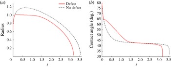
In figure 11, we show the entire time evolution of the radius and apparent contact angle corresponding to the calculations of figure 10. Droplet spreading on a defective substrate behaves identically to droplet spreading on a flat substrate until time
 $t\sim 0.1$
, when the apparent contact line reaches the substrate defect (located at
 $r_{obs}=1.05$
). Afterward, the contact line pins to the side of the defect until time
 $t\lesssim 1.5$
(figure 11
a). While the contact line is pinned, loss of liquid due to imbibition causes the droplet height to decrease, causing the decrease in the apparent angle observed in figure 11(b). (Both the apparent angle and height (not shown) decrease less rapidly when the defect is present.) When the contact angle becomes small enough, approaching the value of the equilibrium angle at time
 $t\sim 1.5$
, the contact line unpins and starts to retract, as shown in figure 11(a). (If the substrate is impermeable, the contact line will remain pinned and the contact angle will remain constant.) Note that during retraction, and right before the end of the imbibition process, the contact angle varies little. This behaviour is qualitatively identical to reported experimental behaviour (Bacri & Brochard-Wyart Reference Bacri and Brochard-Wyart2000; Kumar & Deshpande Reference Kumar and Deshpande2006).
Comparisons of the evolution of the (a) radius and (b) apparent contact angle of droplets spreading on substrates with and without defects. Problem parameters are the same as in figure 10.

Finally, we note that the results of figure 11 indicate that contact-line pinning results in faster liquid imbibition. As seen in figure 10(a), pinning caused by the defect creates a larger curvature of the droplet. This larger curvature generates a higher capillary pressure, increasing the driving force for imbibition. As a consequence, during the time the droplet is pinned, it loses liquid at a faster rate compared to the droplet on the defect-free substrate (which remains unpinned and has a lower curvature (figure 10 a)).
5.3. Comparison with experiments
We now compare predictions of the model with experimental data of PVA/water droplets spreading on permeable substrates (Kumar & Deshpande Reference Kumar and Deshpande2006). In Kumar & Deshpande (Reference Kumar and Deshpande2006), the droplet radius was rescaled with the maximum droplet radius
 $r_{m}$
, and time with the the total imbibition time
 $t_{d}$
. We do the same with the model predictions, and also rescale the apparent contact angle with the initial apparent angle
 ${\it\theta}_{0}$
.
To describe the contact-line pinning observed in the experiments of Kumar & Deshpande (Reference Kumar and Deshpande2006), we collocate a defect just ahead of the initial radius of the droplet. We use the Gaussian depression described in § 5.1 with
 $a=0.35$
,
 $s_{d}=0.06$
and
 $r_{obs}=1.06$
. Since we would like to describe the qualitative features in the experiments of Kumar & Deshpande (Reference Kumar and Deshpande2006) and do not have information about the detailed surface topography in those experiments, the Gaussian defect serves as a convenient (albeit arbitrary) means to account for the influence of surface topography.
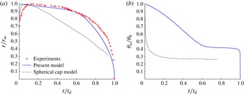
The presence of a defect causes the contact line to rapidly pin to the side of the defect. The results of such a calculation are shown in figure 12 for the case of a PVA/water droplet spreading on a glass fibre mat (this is the same substrate used in the experiment described in figure 7) (Kumar & Deshpande Reference Kumar and Deshpande2006). Also shown are predictions from the spherical-cap model of Starov et al. (Reference Starov, Kostvintsev, Sobolev, Velarde and Zhdanov2002a ).
(a) Experimental measurements (symbols) and model predictions (lines) of the rescaled radius for a PVA/water droplet spreading on a 1.12 mm thick glass fibre mat (case corresponding to UDMAT membrane in figure 11 of Kumar & Deshpande (Reference Kumar and Deshpande2006). The solid line corresponds to the present model with
 $V_{0}=2.7$
,
 ${\it\kappa}=5.6\times 10^{-3}$
,
 $B=0.68$
,
 $b=5\times 10^{-4}$
and
 $\mathscr{A}=0.44/b$
(
 ${\it\theta}_{e}=31.0^{\circ }$
). The dashed line corresponds to predictions of the spherical-cap model shown in figures 7 and 8 of Starov et al. (Reference Starov, Kostvintsev, Sobolev, Velarde and Zhdanov2002a
). (b) Rescaled apparent contact angles corresponding to the calculations shown in (a).

Our model (5.2) is able to reproduce the contact-line pinning observed in the experiments, whereas the spherical-cap model cannot (figure 12
a). We note that corresponding measurements of the contact angle were not reported in Kumar & Deshpande (Reference Kumar and Deshpande2006) and so cannot be compared to the model predictions (figure 12
b), nor were measurements of the effective permeability given. A rough estimate of the dimensional permeability based on our calculations and inferences of the droplet dimensions is
 ${\sim}10^{-7}$
cm
 $^{2}$
, which is within the range of values reported in the literature (§ 4). However, there is considerable uncertainty regarding this value since raw values of the droplet height and contact angle were not reported for the experiments shown in figure 12(a).
Because of the relatively slow rate of imbibition, the contact line remains pinned to the substrate defect for a large fraction of the droplet lifespan. The contact line then retracts relatively rapidly during the last part of the imbibition process. As pointed out by Kumar & Deshpande (Reference Kumar and Deshpande2006), the models of Starov et al. (Reference Starov, Kostvintsev, Sobolev, Velarde and Zhdanov2002a ) and Alleborn & Raszillier (Reference Alleborn and Raszillier2004) could not reproduce this behaviour. Since our model can, we conclude that incorporation of surface roughness is needed to explain the contact-line pinning observed in the experiments of Kumar & Deshpande (Reference Kumar and Deshpande2006).
Our model also provides insight into why poorly wetting liquids pin more easily to rough substrates. Poorly wetting liquids are characterized by larger equilibrium contact angles than strongly wetting liquids. As a consequence, a smaller decrease in the mesoscopic contact angle from some given value would be needed to pin the contact line (recall from figure 10 that pinning occurs when
 ${\it\theta}_{m}$
near the contact-line region is less than
 ${\it\theta}_{e}$
). This observation explains the differences in the behaviour between droplets of high-surface-tension liquids and low-surface-tension liquids that have been reported in the experimental literature. Whereas SO droplets (
 ${\it\sigma}\sim 21~\text{mN}~\text{m}^{-1}$
) do not pin to the substrate and show only an unlocked contact-line behaviour (figures 7 and 8), PVA/water droplets show a locked contact-line behaviour (figure 12,
 ${\it\sigma}\sim 46~\text{mN}~\text{m}^{-1}$
), as do water/glycerol droplets (
 ${\sim}60.2\leqslant {\it\sigma}\leqslant \sim 72.8~\text{mN}~\text{m}^{-1}$
) (Bacri & Brochard-Wyart Reference Bacri and Brochard-Wyart2000) (suction was present in the experiments of Bacri & Brochard-Wyart (Reference Bacri and Brochard-Wyart2000) but is not included in our model).
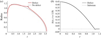
To further illustrate the above observation, we repeat the simulation shown in figure 10 but with a shallower defect (by a factor of five). The shallower defect has a smaller curvature, which does not cause a large enough reduction of the mesoscopic angle near the contact-line region to produce strong pinning, as seen in figure 13. As a consequence, the trajectory of the droplet radius remains close to the trajectory of an identical droplet spreading on a defect-free substrate (figure 13 a). The largest deviation between the trajectory of the two droplets, marked with a cross over the continuous curve, occurs because of the interaction of the contact line with the defect during retraction (figure 13 b). Similarly, other calculations we have performed indicate that if the equilibrium contact angle is made sufficiently large at a fixed defect amplitude, contact-line pinning will occur.
(a) Radius of droplets spreading on a permeable substrate with (continuous line) and without (dash-dot line) a defect when
 $V_{0}=2$
,
 $L=2$
,
 ${\it\kappa}=0.1$
,
 $B=0$
,
 $b=10^{-3}$
and
 ${\it\theta}_{e}=43.3^{\circ }$
(
 $\mathscr{A}=1/b$
). (b) Droplet height at
 $t=1.9$
, marked with a cross in panel (a).

It can also be observed in figure 13 that the imbibition time is slightly longer in the presence of a defect, in contrast to what is observed in figure 11. For the calculations shown in figure 13, the contact-line pinning is not as severe, so the changes to the droplet curvature are more modest. Indeed, for the calculations shown in figure 13, the curvature actually decreases slightly in the presence of the defect, leading to a slightly longer imbibition time.
Finally, we note that if a droplet is spreading on a rough substrate and contact-line pinning occurs, the pinning is likely to be heterogeneous since the substrate topography is. As a consequence, the droplet shape may become non-axisymmetric. An example of this is seen in figure 1, where the droplet spreading on the fibre mat elongates toward the bottom left-hand corner of the images. As a consequence, predictions from an axisymmetric model would not be expected to be in quantitative agreement with data from every (or even most) experiments. Nevertheless, as we have shown above, an axisymmetric model can sometimes still be used to reproduce the contact-line pinning at a maximum radius that is observed in experiments.
6. Conclusions
We have shown that by incorporating surface roughness, lubrication-theory-based models can be used to explain the regime of constant droplet radius that has been observed in experiments of PVA/water droplets spreading on glass fibre mats (Kumar & Deshpande Reference Kumar and Deshpande2006). Our model also uses a modified boundary condition for liquid imbibition that eliminates the need for the ad hoc thickness-dependent permeability employed in previous work. The model can be parametrized by comparing its predictions to experiments on horizontal substrates, and then be applied to other situations where the droplet shape may be far from spherical (e.g. flow down an inclined plane or in the presence of an external airflow).
Although we have considered axisymmetric droplets and isolated defects, our model can readily be extended to account for non-axisymmetric shapes and more complicated surface topography. In this case, it would be of considerable interest to know how substrate permeability modifies the complicated droplet dynamics that have been predicted for droplets on rough impermeable substrates (Savva et al. Reference Savva, Kalliadasis and Pavliotis2010; Savva & Kalliadasis Reference Savva and Kalliadasis2012, Reference Savva and Kalliadasis2013). Another important extension would be to determine whether the approach used here can reproduce the contact-line pinning observed in evaporating droplets, where spherical-cap models are often used. It would also be of considerable interest to couple the model developed here to a model for the imbibition front in the permeable substrate (Starov et al. Reference Starov, Kostvintsev, Sobolev, Velarde and Zhdanov2002a ; Alleborn & Raszillier Reference Alleborn and Raszillier2004; Zadražil et al. Reference Zadražil, Stepanek and Matar2006). Finally, we note that more systematic experiments of droplet spreading on rough permeable substrates are needed, along with measurements of the effective permeability. We are currently conducting such experiments using melt-blown fibre mats like that shown in figure 1 and will report the results in a separate publication.
Acknowledgements
We thank Cummins Filtration for their support of this work. We also thank Dr Z. Wang for providing the images shown in figure 1.
Appendix A. Self-similar solution valid near end of imbibition
As with the model of Davis & Hocking (Reference Davis and Hocking1999), a self-similar solution close to the end of the imbibition process can be obtained for (3.1). For
 $t_{d}-t\ll 1$
, we define
 $$\begin{eqnarray}{\it\tau}=\sqrt{t_{d}-t},\quad h=b+{\it\tau}bf({\it\xi}),\quad {\it\xi}=\frac{r}{{\it\tau}}.\end{eqnarray}$$
An important difference with respect to the approximation described in Davis & Hocking (Reference Davis and Hocking1999) is that the presence of a precursor film of height
 $b$
in our model has to be included in the expansion of
 $h$
.
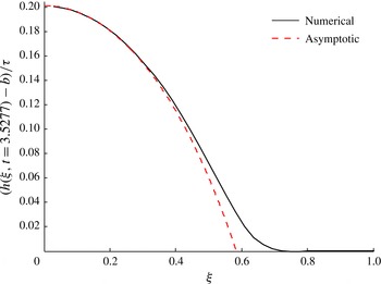
Droplet interface for the case
 $V_{0}=2$
,
 $L=2$
,
 ${\it\kappa}=0.1$
,
 $B=0$
,
 $b=10^{-3}$
, and
 ${\it\theta}_{e}=43.3^{\circ }$
(
 $\mathscr{A}=1/b$
) transformed according to the definitions of (A 1). The dashed curve shows the solution of (A 4), rescaled according to (A 3). For this computation
 $t_{d}=3.529$
.

By replacing the variables defined in (A 1) into (3.1), we find that at leading order in
 ${\it\tau}$
,
 $f$
satisfies
 $$\begin{eqnarray}{\it\kappa}\frac{\text{d}^{2}f}{\text{d}{\it\xi}^{2}}+\left(\frac{{\it\kappa}}{{\it\xi}}-\frac{{\it\xi}}{2}\right)\frac{\text{d}f}{\text{d}{\it\xi}}+\frac{1}{2}f=0,\end{eqnarray}$$
if the extra assumption that
 $b^{3}\ll (t_{d}-t)$
is also satisfied. However, since the value of
 $b$
is typically small, this restriction is mild. By using the change of variables
 $$\begin{eqnarray}x=\frac{{\it\xi}^{2}}{4{\it\kappa}},\end{eqnarray}$$
we can reduce (A 2) to the confluent hypergeometric equation
 $$\begin{eqnarray}x\frac{\text{d}^{2}f}{\text{d}x^{2}}+\left(\frac{1}{2}-x\right)\frac{\text{d}f}{\text{d}x}+\frac{1}{2}f=0,\end{eqnarray}$$
with parameters
 $-1/2$
and
 $1/2$
.
Equation (A 4) has two linearly independent solutions which can be evaluated numerically with the MATLAB commands kummerU and hypergeom. Because of the transformation (A 3), the symmetry condition
 $f^{\prime }({\it\xi}=0)=0$
is satisfied automatically as long as
 $f^{\prime }(x=0)$
is bounded. Thus, we can use the two degrees of freedom to require (A 4) to satisfy
 $$\begin{eqnarray}f(c_{1})=0,\quad f(0)=c_{2},\end{eqnarray}$$
where the constant
 $c_{1}$
is found numerically, and
 $c_{2}$
is used to match
 $h(r=0,t)$
. In figure 14 we show
 $h(r,t)$
transformed according to the definitions of (A 1), at a time close to
 $t_{d}$
, together with the solution of (A 4), shown with a dashed line and rescaled according to (A 3). As seen in figure 14, the agreement between both solutions worsens closer to the contact-line region. This is to be expected since the balance of terms in (A 2), obtained by using the assumption that
 $b^{3}\ll (t_{d}-t)$
, implies ignoring the capillary terms of (3.1).
Appendix B. Computing the mesoscopic angle
The mesoscopic angle, illustrated in figure 15, can be computed using the formula for the tangent of the sum of two angles
 $$\begin{eqnarray}\tan ({\it\theta}_{m}+{\it\gamma})=\frac{\tan ({\it\theta}_{m})+\tan ({\it\gamma})}{1-\tan ({\it\theta}_{m})\tan ({\it\gamma})}.\end{eqnarray}$$
Since
 $\tan ({\it\theta}_{m}+{\it\gamma})=\partial _{r}H=\partial _{r}(h+{\it\eta})$
and
 $\tan ({\it\gamma})={\it\eta}_{r}$
, (5.3) follows.
Schematic illustrating the contact-line region of a droplet on a non-planar substrate. The function
 ${\it\eta}(r)$
describes the substrate height, and the location of the droplet–air interface is given by
 $h(r,t)+{\it\eta}(r)$
.