1. Introduction

Denis Walsh (Reference Walsh2010) has offered the latest in a series of papers advancing a noncausal analysis of evolutionary population genetics (Matthen and Ariew Reference Matthen and Ariew2002; Walsh, Lewens, and Ariew Reference Walsh, Lewens and Ariew2002; Walsh Reference Walsh2007). These previous papers have claimed various virtues for the alternative “statistical” approach, but his current paper does not have much of a positive argument. Rather, Walsh argues, using one of geneticist John Gillespie's equations for fitness (Gillespie Reference Gillespie1974, Reference Gillespie1975, Reference Gillespie1977) and Judea Pearl's works on causality (Pearl Reference Pearl2000), that the causal interpretation of fitness results in a reductio.

Walsh's argument consists of two steps. First, he claims Gillespie's model can generate a Simpson's paradox in fitness distribution; that is, the same genotype can be both fitter in all subpopulations making up a partition of a larger population and, at the same time, less fit in the whole population than the other genotype. Because Simpson's paradox can arise for genuine cases of causation, Walsh needs to invoke an additional reason for rejecting the causal interpretation of fitness.Footnote ¹ For this purpose, his second step invokes Pearl's Sure-Thing Principle (STP; Pearl Reference Pearl2000), which Walsh takes to be a necessary condition for any causal relationship. As, he argues, the fitness distributions generated by Gillespie's model may fail to satisfy this principle, so it follows that fitness cannot be a causal element.

In this reply, we will show that both of these steps contain incorrect assumptions and serious misunderstandings. First, it will be shown that Gillespie's model, correctly understood, does not generate a Simpson's paradox as Walsh suggests. Regarding the second step, we argue that Walsh's application of the STP is based on a misinterpretation of the principle. In the proper reading, there is no violation of the STP and hence no reductio. We conclude that Walsh's argument against a causal interpretation of fitness is unsound.

2. The SS Simpson and the SS Gillespie: Ships Passing in the Night

The first step of Walsh's argument against the causal interpretation of fitness is based on his claim that, under Gillespie's selection model, which explicitly parameterizes population size, alternative descriptions of a given biological population produce fitness distributions that can, in turn, generate a pernicious instance of Simpson's paradox.Footnote ² Before delving into the details, we would like to note that using Gillespie's fitness equations as representative of fitness models is highly idiosyncratic. The fitness measures and models used in the overwhelming majority of population genetics do not include the population size parameter, n, which is essential to Walsh's argument. In fact, Steven Frank and Montgomery Slatkin (Reference Frank and Slatkin1990) have developed a general model that has Gillespie's model as a special case, which does not use the parameter for population size. But setting this aside for the sake of argument, let us examine his case against the causal interpretation of fitness.

Gillespie's equation shows that when there is within-generation variance in reproductive output (i.e., individuals with the same genotype differing in their number of offspring), the fitness of each genotype is measured by the following equation:

where μ and σ² are mean and variance of the number of offspring, respectively; n is population size; and subscript i signifies the ith genotype. Under Gillespie's model, it can be seen that the fitness measure is a decreasing function of n, which means that the genotype, G₁, which is fitter than a competing genotype, G₂, in a larger population, may be less fit in a smaller population. Walsh illustrates this by an example involving two hypothetical genotypes having the following parameters:

He has us imagine, further, a situation involving 14 six-member subpopulations containing both genotypes. Finally, these 14 subpopulations constitute a whole population. Now, according to Gillespie's equation, within each subpopulation j the fitness of G₁ exceeds that of G₂:

where signifies a fitness measure of ith genotype in the jth subpopulation, while, with respect to the population as a whole, G₁ is less fit than G₂;

where the dot subscript means average over subpopulations. Because of this reversal, Walsh concludes that this situation produces a Simpson's paradox: the genotype that is fitter in every subpopulation is nevertheless less fit in the population overall.

There is a serious flaw, however, in the above inference. Walsh's argument presupposes that the means by which we define and partition a biological population is nothing more than a matter of our descriptive interests. He writes, “It is legitimate for biologists to investigate the dynamics of whole populations and their subpopulations; howsoever the latter are demarcated” (Reference Walsh2010, 165; our italics). So how are we to interpret this latter clause? Suppose we have a pregnant female. As the set of all pregnant females (A) is clearly a proper subset of the set of all females (B), this woman is a member of A and, at the same time, of B. In this case, whether we describe this woman as a member of A or of B is completely a matter of our descriptive interest. In a similar vein, Walsh presupposes that insofar as the subpopulation is a proper subset of the whole population, one can describe an organism as belonging to either, and as a consequence, one can calculate, with Gillespie's equation, two different fitnesses for a single organism with respect to the two populations of different sizes.

However, such an assumption ignores what the population size, n, stands for in Gillespie's model. As is explicit in Gillespie's original paper (Reference Gillespie1974, 602), n in his equation is held constant by a density-regulating process, which determines how many juveniles survive and reproduce. The strength of the density-regulating process usually depends on environmental factors, such as habitat condition, abundance and quality of foods, number of predators, and so on. Clearly, then, what determines population size n is not our subjective interest but an objective property of the environment surrounding organisms. The fact that it refers to the objective and concrete parameters, as opposed to our abstract conception of population, is precisely the reason why n matters to fitness, as shown in Gillespie's model. In other words, if the fitness measure of an individual living in a population size of 100 is different from that of an individual in a population size of 500, it is precisely because they are under different density-regulating processes, arising from different sets of environmental factors. This explains why it is meaningless in the above example to calculate two different fitness measures—one for use in a given arbitrary subpopulation and another for use in the whole population—for the same individual. If the subpopulation constitutes the proper environment for the individual, then the proper fitness measure of G₁ is and not , which means, of course, that no fitness reversal arises. Therefore, correctly understood, Gillespie's model does not produce a Simpson's paradox.Footnote ³

As we have shown above, what produced the illusory paradox regarding Gillespie's model was Walsh's illegitimate assumption that biological populations can be demarcated arbitrarily. However, more generally and apart from considerations of Gillespie's model, Walsh's assumption about the arbitrary demarcation of populations is contradicted by the fact that one of the fundamental questions in evolutionary biology is to estimate the effective population size, N_e. A value of N_e reflects crucial aspects of the environment surrounding an organism, which in turn has a particular implication for evolutionary dynamics. Nunney (Reference Nunney1999) has outlined the importance of effective population size and factors involved in measuring it in a variety of contexts. The mere fact that it requires measurement and estimation suggests that it has a real underpinning and that it is not something a biologist can set arbitrarily. Careful estimation of the true effective population size is essential because a significant deviation in the estimation renders the application of a theoretical model to a real biological population completely meaningless. In fact, this point has been the central issue in the famous controversy inaugurated by Ronald Fisher and Sewall Wright and revived recently (Coyne, Barton, and Turelli Reference Coyne, Barton and Turelli1997, Reference Coyne, Barton and Turelli2000; Wade and Goodnight Reference Wade and Goodnight1998; Goodnight and Wade Reference Goodnight and Wade2000)—the dispute over whether evolution takes place in a large panmictic population or small/structured demes. Were Walsh's assumption true and the (effective) population size dependent on nothing more than our descriptive interests, such controversy would lose its entire meaning—an outcome that we suspect Walsh would embrace but that would not do justice to the biologists’ dispute.

Familiarity with Walsh's work provides the means by which to understand why such a confusion about populations and the relationship between alternative descriptions of a population could arise in the first place. A second (and related) difficulty in Walsh's argument concerns causation, specifically with respect to the questionable causal commitments he attempts to burden proponents of the causal interpretation with in Walsh (Reference Walsh2007). More precisely, Walsh makes what he admits is a “substantive assumption” about causation: “Causal relations are description-independent. By this I mean that if x causes y, then this relation holds no matter how x and y are described” (292–93). In order to make his case against the causal interpretation of fitness, Walsh (Reference Walsh2007) describes two interesting simulation experiments that prefigure the Simpson's reversal introduced by Walsh (Reference Walsh2010). The simulations in the 2007 paper involve what he calls a rank order effect (the reversal of rank order given different descriptions of a population). We will briefly describe one such simulation.

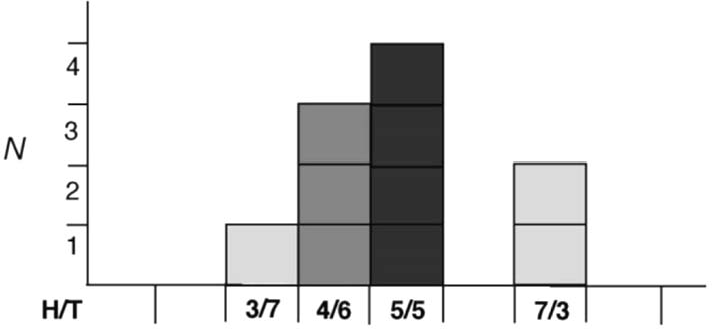
The first simulation, meant to simulate drift, involves tossing two fair coins 50 times each, with 10 experimenters tossing one of the two coins 10 times for a grand total of n = 100 tosses. There are three important analogues here that need to be made explicit in this simulation: the analogue of fitness (of two alleles at a given locus, say) in this simulation is, of course, the probability of a given coin to land either heads or tails; further, the analogue of population size is n, the number of coin tosses; and, finally, the analogue of drift is sampling error, the deviation from expectation. There are, Walsh argues, three equally legitimate ways to describe this simulation and no way to prioritize any of the descriptions over any of the others. What is most interesting about this scenario is that under each of the distinct descriptions, readers are led to draw different (and incompatible) conclusions about the role of drift in the outcome of the simulation. The first alternative is nothing more than a description of the simulation as a single series of 100 tosses of a fair coin, with an outcome of 49 heads and 51 tails. The second alternative is one in which the simulation is described as two (independent) series of a (different) fair coin being tossed 50 times, where the results are 20 heads and 30 tails and 29 heads and 21 tails, respectively. The final alternative is one in which the simulation is described in terms of the experimenters’ tossing of the coins, namely, as a collection of 10 series of 10 coin tosses. It is easiest to describe the results of this last outcome graphically (fig. 1).

Figure 1

Results of coin tossing for 10 series of 10 tosses of a fair coin (Walsh Reference Walsh2007, fig. 1).

Looking back at the three descriptions, recall that Walsh stresses that error, the analogue of drift, varies according to the description of the simulation. With regard to the first alternative, there does not seem to be much deviation from our expectations of the outcome, given that the coins are fair (49 heads and 51 tails vs. the expected 50/50 distribution). Yet, in looking at the second and third alternative descriptions of the simulations, we get quite different stories insofar as we see an increasing trend away from our expectations, with the second alternative of 20 heads and 30 tails and 31 heads and 19 tails versus the expected 25/25 split and with the third alternative deviating from our expectations in 60% of the trials.

At this point, Walsh attempts to drive his point home by drawing attention to the fact that if drift is interpreted causally (e.g., as a means of explaining the deviation from expectation), then it seems that the causal power of drift varies drastically in each of the three cases; in the first instance, there is only a small deviation from expectation, and hence drift is only interacting weakly to produce the outcome, yet, in the third instance, where 60% of the trials deviate from expectation, drift seems to be causally interacting very strongly to produce the outcome. The problem is, of course, that these are not distinct populations being compared but alternative descriptions of the same population. So Walsh seems to present the causal interpretation with a dilemma: either accept the contradiction that drift-the-cause is both strong and weak in the same population or abandon the causal interpretation of drift.

The simulation of selection runs along very similar lines with only a few alterations to the basic setup described above. Here, the probability of a coin landing either heads or tails is the analogue of selection, only this time these probabilities are not equal (the coins are therefore biased, with, e.g., coin 1 having a .6 probability of landing heads and coin 2 having a probability of .4), and, further, the coins to be tossed 10 times by the 10 experimenters are chosen at random. Now, by using the third of the three alternative descriptions discussed above, Walsh is able to produce an outcome identical to the one for drift; namely, that under one such description, the causal power of selection seems to be very strong, and yet, under another, selection does not seem to be playing any role whatsoever in the outcome. Hence, as before, the reader is presented with a dilemma: either embrace a contradiction or abandon the causal interpretation of selection.

The simulations are meant to show that neither drift nor selection are causal on grounds that an alternative description of the situation produces a rank-order reversal in both cases. Walsh's point is a simple one: depending on the particular way that a population is described, it will sometimes appear as if drift has played a significant causal role in the deviation from expectation and, paradoxically, that drift has played little if any role in the same experiment given a different and equally legitimate description of the population. Therefore, the role and strength of drift (and selection) varies in each description, a problematic outcome given that the alternative descriptions are all descriptions of the same population.Footnote ⁴

Looking at the progression of Walsh's work, we see an interesting argument emerging, wherein the proponents of the causal interpretation of fitness are described as being committed to a particular conception of causation, one that entails that causal processes are necessarily description independent. At that point, Walsh produces a series of examples that produce these seemingly counterintuitive and interesting reversals between variables, rank-order reversals in Walsh (Reference Walsh2007) and Simpson's reversals in Walsh (Reference Walsh2010), that makes explicit an apparent tension in the causal interpretation of fitness. The conclusion, then, is that given the apparent correctness of the mathematical operations that produce such a reversal, the only rational thing to do is to abandon the causal interpretation of fitness since the reversals are only paradoxical insofar as we assume that the processes responsible for producing them are causal processes. However, the purpose of this first section was to show that, in fact, there is something wrong with Walsh's interpretation of the mathematical operations involved in producing these reversals, namely, his faulty interpretation of the population-size parameter, n, and his failure to take account of the fact that n is intended to describe the real population in a fixed environment and not any arbitrarily designated population of individuals. With respect to Gillespie's equation, the population of individuals described by n is not, in an important respect, anything at all like the populations of coins Walsh (Reference Walsh2007) describes.Footnote ⁵ Therefore, whereas it is perfectly legitimate to arbitrarily subdivide a population of independent coin tosses, the same cannot be said of a group of individual organisms that make up one biological population in a given environment, precisely because it is that situation and no other which determines the fitness measures for those individuals. In short, one cannot slice up and redescribe a biological population willy-nilly the way one can when describing a coin-tossing experiment since doing so potentially removes a portion of that subpopulation from its all-important ecological context.

However, for the sake of argument, let's grant the possibility of fitness reversals in evolutionary biology and see what, if any, consequences follow for the causal interpretation of fitness. In fact, there are significant instances of fitness reversal occurring within evolutionary biology, a phenomenon that is neither mysterious nor reason enough to reject a causal interpretation of fitness. It is to this topic that we now turn.

3. Simpson Docks with Price (and, by Proxy, Group Selection)

As we have just shown, Gillespie's model does not really produce a case of Simpson's paradox. But there are plenty of cases in evolutionary biology that do seem to produce a fitness reversal; whenever there are multiple levels of selection in operation, there is always a possibility to observe an instance of fitness reversal (Sober Reference Sober1993, 98–102; see also Northcott Reference Northcott2010). As Price (Reference Price1972) showed, in a subdivided population the overall change in a mean trait value, Δz, can be decomposed into (1) the (weighted) average fitness within each subpopulation and (2) the among-populations fitness, as follows:Footnote ⁶

where z is a trait value, w is a reproductive value (e.g., the number of offspring), subscript ij signifies the jth individual in the ith subgroup, dot subscript signifies average, E is average, and Cov is covariance. What this equation tells us is that a trait that has lower fitness in each group (a negative within-group covariance: Cov_j(w_ij / w _i•, z_ij)) may increase in the population as a whole (i.e., Δz > 0), due to high among-group fitness (a positive among-group covariance: Cov_i(w _i• / w _••, z _i•)). This, of course, is the situation that obtains with an examination of altruism, which provides an excellent example. Altruistic individuals are selected against within each group (therefore, these individuals are less fit than selfish individuals) but are favored by group selection, as groups with more altruistic individuals grow faster than those composed of selfish ones. If we denote by w _i,alt, w _i,self the fitness of altruistic and selfish individuals in the ith subpopulation, respectively, and by w _•,alt, w _•,self their overall fitnesses, in the above case we expect

for all subpopulations i, and

for the overall metapopulation, which yields a Simpson's paradox.

So does this conclusion spell disaster for the causal interpretation of fitness? We think not. In fact, on the face of it, what a Simpson's paradox suggests is not that we should deny the causal processes driving selection but rather that there are multiple levels of selection at work. The fitness reversal in group selection is a mathematical fact and is itself neutral to either the causal or the noncausal interpretations of fitness. As we have indicated above, to achieve a reductio of the causal interpretation of fitness from Simpson's paradox, Walsh had to resort to the second step of his argument, the one using Pearl's STP. In what follows, we will examine his argument and explain why, contrary to Walsh's claim, fitness reversals present no threat to the causal interpretation of fitness.

4. Walsh Flirts with Pearl

Walsh's concern for the Simpson's paradox is rooted in his belief that the Simpson's reversal of fitness between two different levels of description (e.g., between a subpopulation and the whole population) entails a violation of Pearl's STP (Pearl Reference Pearl2000, 181), which states:

Walsh construes this principle as a fundamental condition to be satisfied by any causal relationship. According to Walsh, there are some instances of Simpson's paradox that violate this principle, which indicates that the probabilities involved cannot be interpreted causally. A Simpson's reversal of fitness between two different levels of description, in his eyes, falls into the malignant category, and thus he concludes that fitness is indeed not causal at all. As we demonstrated in the first section, Walsh's example fails to produce a Simpson's paradox, yet, as we also showed in the previous section, this kind of reversal does in fact arise in evolutionary biology. Does this mean that fitness is noncausal after all, as Walsh suggests?

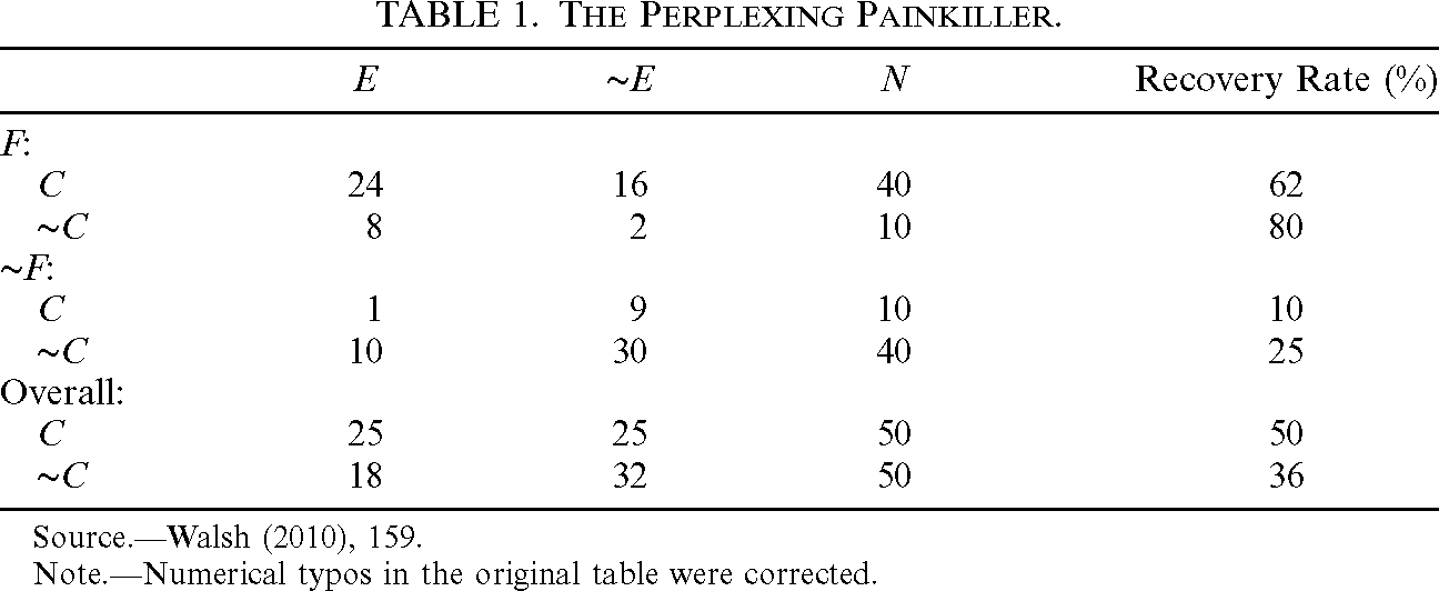
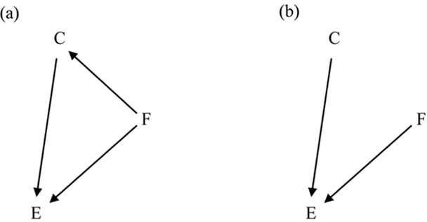
The answer is no. But before jumping to the conclusion, let us recapitulate Walsh's argument. To explain what he means by a violation of the STP, he introduces the example of the Perplexing Painkiller, where administration of a new painkiller drug (C) increases the rate of recovery (E) in both female (F) and male (∼F) subgroups, but the overall data marginalized by gender show that the drug in fact decreases the recovery rate (table 1 of Walsh [Reference Walsh2010], reproduced here as table 1). This is clearly a case of Simpson's paradox since C and E are positively correlated in every subgroup (F and ∼F) while they show negative correlation in the population as a whole. Now, in this case, suppose that the paradox was caused due to F being a confounding factor; that is, males were more prone to take a drug (which indeed is harmful) but were by nature more likely to recover than females. Thus, the gender (F) was indeed the cause of both the drug administration (C) and the recovery (E), and this double-edged effect was the source of the apparent paradox (fig. 2 of Walsh [Reference Walsh2010], reproduced here as fig. 2a). Walsh argues that the Perplexing Painkiller example violates STP, given that “an action, C (administering the drug), that increases the probability of nonrecovery, ∼E, in each subpopulation decreases it overall,” while the same action does not change the distribution of the subpopulation—that is, taking a drug does not affect the gender (F). From this “violation,” he concludes that this example presents “an incoherent set of causal beliefs” (Reference Walsh2010, 162).

Table 1The Perplexing Painkiller.

	E	∼E	N	Recovery Rate (%)
F:
C	24	16	40	62
∼C	8	2	10	80
∼F:
C	1	9	10	10
∼C	10	30	40	25
Overall:
C	25	25	50	50
∼C	18	32	50	36

Source Walsh (Reference Walsh2010), 159.

Note Numerical typos in the original table were corrected.

Figure 2

Causal relations of the Perplexing Painkiller example before (a) and after (b) intervention on treatment, C.

But is there really a violation? What is crucial in Pearl's STP, but completely ignored in Walsh's discussion, is that Pearl's motivation and use of this theorem is concerned with causal calculation (his do calculus) and not with ordinary probabilistic calculation. For example, “An action C increases the probability of an event E” translates to P(E|do(C)) in Pearl's notation, which is different from the mere conditional probability P(E|C). Pearl's do calculus concerns the possible or counterfactual probabilistic distribution induced from a particular manipulation of the causal model, not the actual frequency observed in the data. Regarding our example, what is at issue is not the conditional probability that a person recovers given that we observe she or he took a drug but the probability of her or his recovery that would be obtained if we intervene and make the person take the drug. With this distinction in mind, Pearl's STP reads as follows:

Sure-Thing Principle (STP).

To examine whether the Perplexing Painkiller example really violates this principle, we need to specify the value for each term in the above formula. The probability distribution induced by an intervention is obtained with the aid of a directed acyclic graph (DAG) that represents the causal relationship after the intervention. The DAG resulting from the intervention on drug administration (C) is shown in our figure 2b. The new probability distribution is obtained by multiplying the observed conditional probabilities of each node given its parents in the new DAG (Pearl Reference Pearl2000, 72). Applying Pearl's do calculus to Walsh's probability distribution in table 1 and causal structure in figure 2b yields in each gender

and the overall distribution (marginalized by gender)

Therefore, the example shows no violation of STP; that is, the administration of the drug (C) decreases the probability of recovery (F) both in each subpopulation and in the population as a whole.

We have just shown that there is no violation in the Perplexing Painkiller example. But this result can be generalized: there is no such thing as “violation” of the STP. After a little thought, this is obvious. Pearl's do calculation works only when a definite causal model is given as one of its inputs; as such, the result of the calculation cannot be inconsistent with its premises (unless, of course, the calculation itself is defective). This means that from the STP alone we cannot judge whether our causal beliefs are true, let alone whether they are causal or noncausal.Footnote ⁷ The alleged violation of the STP results only from the equivocal interpretation of the probability term appearing in the principle, taking the proviso as a statement about do calculus and interpreting the inner conditional as being about ordinary probability. Once the STP is interpreted correctly and coherently in terms of causality (i.e., Pearl's do calculus), there will be no violation whatsoever, and, as a consequence, Walsh's attempt to construct a reductio of any sort—either with his Perplexing Painkiller example or with the causal interpretation of fitness—is doomed to fail.

As we have seen above, Pearl's STP is to be read entirely in terms of his do calculus, that is, causal probability. Meanwhile, we can also read the STP in an entirely probabilistic way, yielding the following “ordinary” probability version:

Taken as such, this proposition simply reveals a necessary condition for the Simpson's paradox, namely, that it arises only if C and F_i's are dependent. Again, this brings no incoherence to our example above, as clearly the proviso (independence of drug administration, C, and gender, F) is not met. Both of Walsh's examples show biased sampling and thus correlation between C and F.

It is also interesting to note that PSTP is consistent with our case of group selection, wherein the proviso is tantamount to saying that the distribution of the trait in question is independent of its grouping. This will make the among-group variance and hence among-group covariance (Cov_i(w _i• / w _••, z _i•)) zero. Then from the rest of the equation, we clearly see that at least one of the within-group covariance values must have the same sign as the total covariance. In the case of altruism, if every subpopulation contains the same proportion of altruists and individualists, the subpopulations do not differ in their “group trait,” and thus no group selection occurs. The total change in frequency in this case should reflect only within-group fitness; that is, altruists should decrease both in the subpopulations and the whole population—this would produce no Simpson's paradox and thus no violation of PSTP.

5. Conclusion

Walsh argues that causation conforms to the STP and that fitness distributions do not; therefore, fitness distributions are not causal. If there were causal processes occurring within natural selection, then those processes ought to be description independent; that is, the outcome of any description of an evolutionary process ought to remain the same, irrespective of how we describe that process, according to Walsh. For instance, in Walsh's coin example, we would infer that, given the three alternative descriptions of the population described above, selection (or drift) either did or did not play a substantive role in the production of the (simulated) outcome since, under one description, it seems as if selection (or drift) played a predominant role in the outcome, while, given another (equally legitimate) description, it seems as if selection (or drift) played almost no causal role in the outcome described. Walsh's point is that in the event that alternative descriptions alter either the presence or the strength of the alleged causal properties/processes, then there are no actual causal properties/processes doing any real work within that system.

However, regardless of the occurrence of reversals in (re)descriptions of coin-sampling experiments, we showed that Gillespie's model of selection does not generate a Simpson's reversal, much less a paradox of any kind. This is because Gillespie's population size, n, is not a mere statistical/descriptive summary that is dependent on our interests at the time but has a real biological meaning and significance, one that cannot be divorced from the notion without serious harm being done to the interpretation of the model.

Further, we showed that the Price equation is capable of describing the conditions under which a Simpson's paradox really does seem to arise in the context of evolutionary biology. Nevertheless, even this occurrence fails to produce the result that Walsh intended, namely, a violation of Pearl's STP. In fact, such a violation is an illusory result due to the misapplication and misinterpretation of the principle. If Pearl's principle is understood consistently, as we have outlined above, then no such violation arises, regardless of whether STP is interpreted causally or purely probabilistically.

In closing, then, while it is left an open question as to whether fitness ought to be interpreted in a causal manner, Walsh's arguments for rejecting the causal interpretation of fitness founder on the shoals. As we have shown, his arguments against the causal interpretation depend too heavily on a defective interpretation of biological population, one that misinforms his reading of Gillespie's model of selection. Furthermore, Walsh has failed to produce the claimed Simpson's paradox and violation of the STP, which constitute the core of his criticism of the causalists’ position.