





Nomenclature
- a
-
Airframe-instance index (component label) in a GSE-airframe pairing ((g,a)). Also, the argument of the per-class thickness prior (t(a)).
- BA
-
Bland-Altman analysis/plot used to characterise pixel-level depth agreement and bias.
- CI
-
Confidence interval.
- CNN
-
Convolutional neural network.
- d_{xy}(g,a)
-
Minimum boundary-to-boundary ground-plane (XY) distance between a GSE instance (g) and an airframe instance (a).
- DA-V2
-
DepthAnything-V2 depth-estimation model.
- f_x, f_y
-
Camera focal lengths in pixel units (intrinsics) used in the projection model.
- GSE
-
Ground Support Equipment.
- H(u,v)
-
Estimated height above ground at pixel ((u,v)), computed as (H=H_c - Z(u,v)).
- H_c
-
Calibrated camera height above the ground plane.
- IoU
-
Intersection over Union (mask overlap metric).
- ISP
-
Image signal processor/image signal processing.
- K
-
Number of clusters used for GSE in-mask height envelope estimation.
- MAE
-
Mean absolute error (depth), in metres.
- MRO
-
Maintenance, Repair and Overhaul.
- Q_{95}
-
95th percentile operator (used for robust ``top’’ height extraction).
- RMSE
-
Root mean square error (depth), in metres.
- t(a)
-
Per-class vertical-extent (thickness) prior for airframe instance (a), used to estimate underside height.
- SfM
-
Structure from Motion
- SLAM
-
Simultaneous Localisation and Mapping
- UWB
-
Ultra-wideband positioning.
- Z(u,v)
-
Metric depth at pixel ((u,v)), in metres.
- Z-gate
-
Vertical plausibility test that checks overlap between GSE top-envelope heights and airframe underside height.
- YOLO
-
You Only Look Once (real-time detection/segmentation family) NN model for object detection and instance segmentation.
Greek symbol definition
- δ
-
(i)
 $\delta $
-threshold depth accuracy criterion using
$r={\max}(\hat{z}/z, z/\hat{z})$
with
$\delta \lt 1.25,{1.25^2},{1.25^3}$
; (ii)
${\delta _z}$
is the slack margin used in the Z-gate.
- κ
-
Cohen’s kappa for annotation agreement (reported as
$\kappa \gt 0.9$
).




1.0 Introduction
Ground handling incidents involving aircraft and ground support equipment (GSE) remain a major operational and financial burden in aviation maintenance, repair and overhaul (MRO). The International Air Transport Association estimates the combined direct and indirect cost of ground-based incidents at approximately $5.5B in 2022, with projections approaching $9.7B by 2035 without further preventative measures [1]. Beyond repair cost, these events create substantial disruption, as damaged aircraft can remain unavailable for multiple days [Reference Cook2–Reference Kromphardt4]. Safety reporting also indicates that human factors dominate; NASA ASRS attributes over two-thirds of such occurrences to human performance errors [5], and the International Business Aviation Council reports that 71% of aircraft damage arises from collisions with ground equipment or static objects, with 57% occurring while aircraft are parked under ground handling activities [6].
This has accelerated interest in sensor-enabled ground operations and, in particular, unpiloted or minimally supervised GSE [Reference Zhang, Zhang and Zhu7]. Such platforms typically rely on multi-sensor perception (e.g. cameras, LiDAR, radar) with learned object recognition for environment understanding and safe motion planning [Reference Dyer and Thesis8, Reference Casey9]. Hangar environments present a distinct constraint set compared with open-ramp operations: GNSS and ground radar coverage may be degraded, aircraft structures create tight clearances (notably around the nacelle and empennage) and the operational scene contains numerous heterogeneous assets that are frequently repositioned. Practical collision-risk monitoring therefore requires (i) reliable recognition of aircraft components and nearby equipment and (ii) a means of estimating clearance in real time to support operator warnings and provide a machine-readable risk state, e.g. ‘clear/warning/alert’ that could be integrated into future vehicle or facility safety interlocks. Among available sensing options, monocular red-green-blue (RGB) cameras are attractive for scalable hangar deployment: they are low-cost and lightweight, and they provide rich semantic information for recognising aircraft features and maintenance-centric GSE when paired with appropriate optics and illumination [Reference Mallik10].
The central technical challenge is that monocular imagery does not directly measure range. This study, therefore, investigates whether a monocular workflow can be made viable for hangar collision-risk monitoring by combining (i) instance segmentation of aircraft components and GSE and (ii) learned metric depth inference, integrated with explicit geometric decision logic. To achieve this, (iii) the construction of a domain-specific dataset (Fig. 1) is implemented for hangar viewpoints and ontology, combining synthetic renders with matched miniature-testbed imagery to enable training and evaluation in an MRO-relevant setting.
Overview of MRO hangar environment.

The study is structured around three research questions: (RQ1) whether a synthetic workflow, parameterised with camera intrinsics matching the physical miniature-testbed setup, can train monocular segmentation and depth models for a top-down MRO viewpoint; (RQ2) whether known 3D-printed calibration objects can provide a defensible proxy evaluation of testbed-image depth-structure behaviour when dense real-depth ground truth is unavailable; and (RQ3) whether learned masks and depth can be converted into interpretable geometric quantities suitable for collision-risk warning logic.
The contribution is therefore not a claim of certified autonomous collision avoidance. Rather, the study presents a traceable perception-to-geometry framework, together with a physically executed miniature-testbed validation step that defines what the monocular approach can and cannot currently support. In particular, the miniature-testbed depth results provide structural/ordinal rather than clearance-grade absolute metric validation.
The remainder of this study is organised as follows: Section 2 reviews existing hangar collision-prevention practices and summarises the sensing and perception literature most relevant to monocular clearance reasoning. Section 3 details the proposed framework, including camera configuration, dataset construction using paired simulated-environment renders and miniature-testbed imagery, training and evaluation of the segmentation and metric-depth models and the deterministic collision-inference logic. Section 4 reports quantitative results for depth and segmentation, together with end-to-end clearance and alert outputs demonstrating traceability of the inferred risk state. Section 5 concludes with key findings and recommendations for scaling validation and calibrating safety thresholds for representative MRO deployment.
2.0 Background
2.1 Existing collision prevention practices and systems
Operational mitigation has historically been procedural, with safety management systems and standard operating practices designed to reduce GSE–aircraft contact events [6]. While such measures reduce risk, incidents persist even under supervised moves and controlled procedures [Reference Smith11]. In parallel, technology aids have been introduced to provide proximity awareness and automatic warning/slowdown functionality. Examples include vehicle-mounted radar proximity sensing integrated by some manufacturers [12] and multi-sensor warning products such as WingGuard, which uses multiple sensors and an operator display to indicate proximity hazards [Reference Smith11]. At the hangar level, collision prevention has also been explored through infrastructure-heavy monitoring and multi-sensor fusion. A representative example is the Smart Hangar concept, which fuses cameras, 3D LiDAR and ultra-wideband (UWB) sensing to maintain a real-time digital twin, track assets and personnel and issue collision-prediction alerts [Reference Casey9]. These approaches demonstrate what is achievable with abundant sensing, but they also introduce significant integration complexity and cost (multiple modalities, calibration, fusion, maintenance), which can be a barrier to broad deployment across diverse MRO facilities.
2.2 Sensor modalities for object detection in ground operations
Cameras provide strong semantic capability for object recognition and classification and are attractive for widespread deployment due to cost and form factor [Reference Wei, Ding and Li13]. Their limitation is the absence of direct range measurement in the monocular case and their sensitivity to lighting artefacts, such as glare and shadows [Reference Liu, Wu and Wang14, Reference Dubois15]. Active ranging modalities address this: LiDAR provides accurate geometric point clouds and works independently of ambient illumination [Reference Dubois15], offering clear benefits for clearance measurement in tight manoeuvres [Reference Liu, Wu and Wang14], but it remains comparatively expensive and can be sparse depending on the configuration. Radar is robust to adverse visibility and lighting and provides reliable coarse ranging [Reference Guan, Madani, Jog, Gupta and Hassanieh16], but it generally lacks the spatial detail required to resolve fine clearances around complex aircraft geometry [Reference Marchetti17, Reference Jiang, Guo, Luo, Yao and Cui18]. Positioning approaches (e.g. RFID/UWB) can provide asset locations in a tracked environment [Reference Wang, Che, Zhao and Lim19, Reference Al-Okby, Junginger, Roddelkopf and Thurow20] and have been used within fused digital-twin concepts [Reference Casey9], but their accuracy is typically insufficient alone for near-contact clearance checking, and they are commonly used as one component of a broader system.
As a result, many high-reliability solutions adopt sensor fusion (e.g. vision for semantics in addition to radar/LiDAR for range) [Reference Liu, Wu and Wang14]. However, each added sensor increases cost and integration burden. This motivates investigating whether a single-sensor approach, using vision in particular, can be extended to support both recognition and clearance estimation sufficiently for hangar collision-risk monitoring.
Table 1 summarises the main sensor-modality trade-offs for aircraft-hangar collision-risk monitoring. The comparison does not treat monocular vision as inherently superior to active ranging. Instead, it clarifies the deployment trade space: LiDAR and radar provide direct ranging or strong environmental robustness but introduce cost, integration, spatial-resolution or semantic-interpretation trade-offs; positioning systems support asset localisation but do not directly resolve surface-to-surface aircraft clearances [Reference Casey9, Reference Guan, Madani, Jog, Gupta and Hassanieh16, Reference Al-Okby, Junginger, Roddelkopf and Thurow20–Reference Masoumian, Rashwan, Cristiano, Asif and Puig22]. This motivates the present monocular-RGB camera-first framework as a low-infrastructure proof-of-concept for jointly estimating aircraft/GSE semantics and clearance-relevant depth, while preserving the limitation that operational safety deployment may require uncertainty-aware thresholds or sensor fusion.
Qualitative comparison of sensing modalities for hangar collision-risk monitoring

Table 1. Long description
Table with four columns and multiple rows comparing different sensor modalities for aircraft hangar collision risk monitoring. Columns include Clearance-Resolution, Spatial Resolution and Lighting/Environmental Relevance, Modality Cost/Integration Burden, and Semantics Robustness. Each row details a specific sensor modality such as Monocular RGB camera, Stereo or RGB-D camera, LiDAR, Millimetre-wave radar, RFID/UWB positioning, and Fused digital-twin sensing system. Each modality is evaluated across the four columns with detailed descriptions of their characteristics and implications for the study.
2.3 Vision-based object recognition and collision avoidance
Vision-based perception has been widely explored for airport and ground-operation tasks, as it can be deployed with minimal infrastructure and can provide detailed scene interpretation. Monocular vision is especially appealing due to its simplicity; reliable depth inference from a single view, however, remains challenging [Reference Wei, Ding and Li13]. Early airport-domain work often targeted narrow problems, such as docking alignment, and relied on carefully engineered vision pipelines, limiting generalisability across operating conditions [Reference Perez, Mendiolagoitia, Blanco and Alvarez41, Reference Casado Merino and Bermejo42]. More recent work uses deep learning detectors (e.g. YOLO-family networks) for recognising ground vehicles and obstacles, including work targeting unpiloted GSE where real-time detection is essential for preventing collisions [Reference Zhang, Zhang and Zhu7]. While detection addresses ‘what is present’, collision avoidance requires ‘how far’, and many systems introduce an additional ranging sensor once an object is identified, thereby reducing the attractiveness of a strictly monocular solution.
Depth estimation from monocular imagery has been approached via multi-view geometry (SfM/visual SLAM) [Reference Wei, Ding and Li13], and these methods are often computationally heavy for real-time operation on high-resolution streams [Reference Xiang, Chen and Ji43] and typically yield sparse reconstructions that may be inadequate for clearance monitoring across an entire scene [Reference Matsuki, Scona, Czarnowski and Davison44]. Deep learning has enabled single-image dense depth prediction [Reference Yang, Kang, Huang, Xu, Feng and Zhao45], including self-supervised approaches such as Monodepth2 [Reference Godard, Mac Aodha, Firman and Brostow46], and has demonstrated utility in mobile robotic settings [Reference Almagro47]. Several authors argue that low-cost RGB cameras can support obstacle avoidance through learned depth inference, reducing reliance on relatively expensive active sensors [Reference Florea, Miclea and Nedevschi48, Reference Filho, Cabral, Givigi and Nascimento49]. However, hangar environments differ materially from the dominant training distributions of many well-known datasets used for vision models (lighting, reflections, large smooth airframe surfaces, extreme scale differences between GSE and aircraft), and collision-risk monitoring additionally imposes strict latency constraints for timely warning or intervention.
2.4 Limitations of previous work and key contributions
The literature indicates a trade space: multi-sensor and infrastructure-heavy systems can achieve comprehensive awareness (e.g. Smart Hangar fusion of cameras, LiDAR and UWB) [Reference Casey9], but at a relatively high complexity and cost; vision-only systems have often been either task-specific (e.g. docking sub-problems) or insufficiently validated for safety-critical hangar operation at scale [Reference Zhang, Zhang and Zhu7]. More broadly, limitations in tracking precision and automation remain recognised challenges in airport ground safety contexts [Reference Wang, Che, Zhao and Lim19]. Consequently, despite recent progress in monocular perception, there remains a practical gap: a demonstrated, aircraft hangar-tailored monocular framework that jointly (i) recognises both aircraft components and repair-MRO-relevant GSE and (ii) provides clearance-relevant depth characterisation with real-time feasibility. This study targets that gap through a monocular depth-segmentation pipeline and a dedicated dataset designed around hangar viewpoints and ontology.
3.0 Methodology
3.1 Framework and scope
This work demonstrates a monocular vision pipeline for collision-risk monitoring during hangar-based MRO operations, where equipment manoeuvres occur under tight clearances and infrastructure-heavy sensing (e.g. LiDAR networks, UWB tagging) can be impractical to deploy or maintain at scale. The methodology proceeds from (i) requirements definition, to (ii) camera configuration and placement for hangar viewpoints, to (iii) novel dataset construction combining synthetic and physical miniature imagery, to (iv) training and evaluation of segmentation and metric depth models and finally to (v) integration into a clearance-checking and alerting pipeline. The system has two core functions:
-
1. Perception: recognise and segment aircraft components and GSE in overhead monocular imagery and infer metric depth.
-
2. Decision: convert perception outputs into clearance estimates and collision-risk alerts using explicit geometric logic.
The current implementation targets two high-risk GSE classes (forklift, scissor lift) and two maintenance-critical aircraft regions (nacelle, empennage), selected to represent high-value structures and frequent maintenance proximity operations.
3.1.1 Requirements analysis
A preliminary hazard analysis identified aircraft-GSE contact as a dominant risk during towing and line-maintenance activities. Interviews with MRO engineers and safety officers were complemented by incident log reviews [50], yielding four core functional requirements:
-
• Continuous perception of GSE within close vicinity of the airframe
-
• Metric clearance estimation within a reasonable operational radius about the airframe
-
• Low latency suitable for real-time warning
-
• Modular deployment tolerant of heterogeneous hangar layouts, with minimal wiring and unobtrusive installation
Risk quantification employed a severity-frequency matrix in which each GSE class (tug, scissor lift, high-loader, forklift, maintenance stand) was ranked according to historical incident rates and potential damage costs. These rankings motivated the initial focus on forklifts and scissor lifts and the use of nacelle and empennage viewpoints as representative high-consequence MRO collision contexts.
3.1.2 System overview
The proposed monocular vision collision avoidance (MVCA) system comprises three coupled subsystems:
-
• Perception layer: ceiling-mounted RGB cameras provide image streams to an on-premises edge server (nominally 30 fps).
-
• Inference layer: a dual-head architecture produces (i) instance masks and class labels, and (ii) a dense metric depth map.
-
• Decision layer: post-processing combines and converts depth-segmentation tuples produced by the two separate models into metric clearances and collision-risk states (clear/warning/alert) using explicit geometric checks.
Rationale for modular separation: the design isolates learning-enabled perception from deterministic decision logic to reduce the re-certification burden when models are updated [Reference Gleirscher and Kugele51]. This aligns with modular safety arguments for learning-enabled components [Reference Heidemann, Kurzidem, Monnet, Roscher and Günnemann52] and mitigates operational disruption from dataset drift or lighting changes that may require periodic re-training [Reference Ferreira, Guérin, Delmas, Guiochet and Waeselynck53].
Camera ISP constraint: the pipeline avoids reliance on tightly tuned integrated ISPs, as common ISP optimisation targets may not track CNN performance [Reference Hansen54], model features can entangle with ISP parameterisation [Reference Molloy55], and tuning variation can induce false negatives, which are unfavourable in safety-critical perception [Reference Molloy55]. Explicit intermediate outputs (masks and depth maps) improve debug traceability [Reference Heidemann, Kurzidem, Monnet, Roscher and Günnemann52] and support structured artificial intelligence safety-case arguments [Reference Habli56].
3.2 Methodology details
3.2.1 Sensor suite design
A survey of stereo, structured-light and LiDAR options was conducted. A monocular industrial RGB configuration (Basler camera and lens combination) was selected to prioritise deployability and scalability in an MRO hangar setting. Each unit was paired with a lens selected to minimise distortion across the usable image height (as verified by image height vs. distortion plots for the chosen sensor/lens pair). Minimising distortion was treated as a control variable since the same intrinsics/extrinsics are mirrored in the synthetic rendering pipeline, improving synthetic-to-miniature-testbed correspondence.
The selected configuration yields a ∼33° horizontal field-of-view. For a representative hangar ceiling height of 28 m, the ground footprint is approximately 16.6 m horizontally (and ∼12.4 m vertically at the corresponding vertical field of view (FOV)), sufficient to cover the intended maintenance-critical zones (nacelle and empennage) while avoiding excessive perspective compression (Fig. 2).
Field of view obtained in the current methodology’s camera outputs.

3.2.2 Sensor placement optimisation for dataset creation
Camera locations were selected to represent collision-relevant viewpoints while avoiding systematic visual artefacts that inflate false collision risk. Positioning directly above the fuselage centreline produced perspective-induced occlusions in which GSE silhouettes merged with the fuselage in the 2D image plane despite physical separation. This artefact increased segmentation error and generated false-positive collision detections in the downstream decision logic. Cameras were therefore offset laterally from the centreline such that the viewing frustum cleared the wing/fuselage intersection while preserving coverage of the nacelle and empennage. The required offset is computed once the aircraft type and target maintenance zones are known.
3.2.3 Controlled validation testbed and calibration objects
Prior to full-scale deployment, a scaled physical mock-up (miniature testbed) was constructed to validate end-to-end feasibility under controlled yet realistic imaging conditions. A fixed twin-engine, twin-aisle transport-aircraft scale model, matched to the airframe geometry used in the synthetic BlenderProc2 scenes, was positioned alongside 3D-printed forklifts and scissor lifts (Fig. 4). Cameras matching the production configuration were mounted at scaled heights to emulate ceiling installation. Adjustable LED lighting replicated representative hangar illumination to test robustness against shadowing and highlight variations. The aircraft-geometry assumptions and underside priors are therefore specific to this test geometry and are not claimed to be aircraft-type invariant.
Since the target deployment in the miniature testbed employs RGB cameras exclusively, the methodology validates metric depth behaviour via controlled geometric structures. During inference, predicted depth over each structure’s planar faces is assessed for (i) planarity, (ii) consistency with expected distance/height and (iii) stability across pose/lighting perturbations. This provides an operationally relevant metric-depth sanity check when direct pixel-level ground-truth depth is unavailable in real imagery.
3.2.4 Depth-calibration objects
To operationalise monocular depth-cue testing in a top-down hangar-like viewpoint, a set of structures was designed to (i) emulate six DepthCues probes (elevation, light/shadow, occlusion, perspective, size, texture gradient) [Reference Danier, Aygün, Li, Bilen and Mac Aodha57], and (ii) remain fully visible under the selected camera FOV and mounting geometry. The same nominal structures are represented in the Blender scenes and 3D-printed for the miniature testbed, allowing real-camera validation to evaluate surfaces whose nominal geometry is known. As listed in Table 2 and shown in Fig. 3, the calibration-object set comprises the horizontal half-cylinder (c), the same object rotated so that its flat surface faces the camera, referred to as the vertical half-cylinder (c90), the step-cube objects (d, s) and the ‘truck’ composite (t). The testbed-image metric-depth validation uses C90 as a planar/elevation sanity check and uses step-cube object D and step-cube object S as structured height-discontinuity probes.
For the miniature-testbed images, manual polygon labelling is required since the cameras supply RGB imagery rather than dense measured depth. The labels define where each known calibration-object surface appears in the image, allowing the inferred depth to be sampled from the correct physical patch and compared with the corresponding nominal surface height. Each polygon is drawn inside a single surface patch to avoid boundary pixels, shadows and occlusions as far as practicable; visibility flags are retained for quality control and primary metrics are calculated from clear regions (Fig. 10, top left). The nominal geometry of each labelled surface is expressed relative to a local floor datum. The model-output convention and conversion from miniature dimensions to model-domain metres are specified with the metric-depth evaluation procedure in Section 3.2.7, where these labels are used to form the proxy error metrics for real RGB imagery.
Structural depth-calibration models description

Table 2. Long description
Panel A: Diagram of a horizontal half-cylinder with a curved side up, showing a continuous depth gradient. Panel B: Diagram of a vertical half-cylinder with its axis orthogonal to the horizontal half-cylinder, demonstrating a controlled test of apparent height versus distance. Panel C: Diagram of a step-cube object with a 40 by 20 mm base and eight extrusions at 15-20 mm increments, creating known depth discontinuities and self-occlusions. Panel D: Diagram of a truck composite object, which is a half-cylinder fused to a rectangular cuboid, challenging the model to reconcile conflicting depth cues within a single object.
Depth-calibration models: (a) dimensional example of a step-cube object (mm) and (b) the 4 calibration object types.

3.2.5 Dataset acquisition and generation
This work contributes a domain-specific dataset for monocular hangar perception, referred to here as the Hangar dataset, constructed to support:
-
• MRO-relevant object ontology (airframe subcomponents + GSE classes)
-
• top-down ceiling viewpoints
-
• paired synthetic RGB-depth mask exports
-
• matched real miniature imagery for domain shift evaluation
Campaigns captured images containing aircraft components, GSE and (for the purpose of metric depth inference evaluation) calibration objects. A stratified protocol ensured representation across (i) the two target GSE classes and (ii) the two aircraft viewpoint zones (nacelle/empennage).
Miniature-testbed images. (a) Left: camera hardware mounted on testbed hangar structure; (b) Right: resulting top-down RGB capture of forklift and scissor lift relative to aircraft fuselage model. The setup replicated production camera intrinsics, lens distortion and ceiling lighting.

Synthetic data generation: a simulated-environment pipeline, BlenderProc2 [Reference Denninger58], was used to generate 2,800 physically plausible scenes with randomised object poses while enforcing collision constraints (Figs 1 and 2). Camera intrinsics/extrinsics mirrored the physical miniature-testbed setup and used the same fixed twin-engine transport aircraft and GSE geometries in the physical testbed. For each synthetic image, the pipeline exports pixel-aligned metric depth, normals and instance labels automatically. The synthetic evaluation split is scene-disjoint from training: the retained depth-training script reads paired samples from separate train and validation samples, while the reported synthetic depth and collision evaluations use held-out scene dataset samples that were not used for fitting.
3.2.6 Instance segmentation
Instance segmentation is evaluated for the top-down aircraft-hangar scene in which each image contains one airframe component of interest and one or two GSE objects (forklift(s) and/or scissor lift(s)). Inference uses a six-class ontology (background excluded): elevator, forklift, fuselage-wing, nacelle, rudder, scissor lift.
Ground-truth instance masks are implemented and defined as polygon annotations and rasterised to dense masks (background = 0). Polygon quality is controlled via a two-pass consensus workflow. Inter-annotator agreement is enforced at Cohen’s κ
 $\gt$
0.9, and disputed regions were resolved during the second pass before final rasterisation.
YOLOv8 segmentation variants (nano, small, large, xlarge) [Reference Jocher, Chaurasia and Qiu59] are trained using 400 images in total: 300 simulated environment renders (from two virtual camera locations) and 100 miniature testbed images captured from the GSE-containing miniature setup (no 3D calibration objects present in this segmentation subset). Predicted instance masks are composited into a per-pixel class-ID map for evaluation.
Performance is reported using two complementary non-background Intersection over Union (IoU) summaries. Aggregate micro-IoU is computed as the sum of foreground-class intersections divided by the sum of foreground-class unions across the evaluated split. Mean IoU and the associated 95% confidence intervals in Tables 4–7 are computed over per-image IoU values using 10,000 bootstrap resamples. Compute Unified Device Architecture (CUDA)-synchronised inference timing is reported as median interquartile range (IQR) to reduce sensitivity to first-call warm-up effects.
Qualitative outputs (Figs 15–18) include:
-
• error maps (correct, false positive, false negative, misclassification)
-
• boundary overlays comparing predicted vs. ground-truth contours
3.2.7 Metric depth
Metric depth is evaluated through two complementary evidence streams based on whether inference is implemented on real or simulated synthetic scenarios. The first stream uses labelled calibration-object surfaces in the miniature-testbed RGB images to provide a testbed-image proxy validation, since the physical RGB cameras do not provide dense measured depth. This real-image stream is interpreted as ordinal/structural transfer evidence only; it is not treated as absolute metric-depth validation for clearance-threshold decisions. The second stream uses dense synthetic ground truth from the camera-matched BlenderProc2 scenes to quantify pixel-wise depth accuracy under controlled conditions. Both streams use the same model-output convention: the monocular depth head estimates camera-axis metric depth, which is converted to height above the local floor datum before clearance reasoning is applied.
-
a) Miniature calibration subset (testbed imagery): The RGB-image proxy validation uses the labelled calibration-object surfaces introduced in Section 3.2.4. For each labelled polygon, the inferred camera-axis depth is converted to height above the local floor datum and reduced to a robust median over conservative interior pixels. This predicted height is compared with the nominal surface height after converting the miniature-object dimensions from millimetres to model-domain metres using the 100x scale convention. The resulting signed and absolute patch errors are reported diagnostically, while the study-level inference from real imagery is limited to whether the model preserves the known ordering and relative structure of the stepped surfaces. Step-cube objects are therefore additionally evaluated using pairwise step differences and monotonic step-order accuracy, which tests ordinal/structural transfer rather than clearance-ready absolute metric accuracy.
-
b) Synthetic dataset (BlenderProc2): Depth ground truth is inherited directly from the BlenderProc2 pipeline outputs. These are stored as HDF5 files containing aligned RGB and metric depth. The synthetic evaluation stream is therefore structured around three linked subcomponents: the evaluation split and valid-pixel mask; the matched comparison between the custom and public pre-trained DepthAnything-V2 models; and the metric/diagnostic reporting used to quantify accuracy, uncertainty, bias, range sensitivity and failure cases.
Evaluation split and validity mask: Quantitative model evaluation is conducted on the synthetic test split. The depth maps are spatially aligned to RGB at native resolution. Only valid pixels are evaluated. A pixel is considered valid only if its depth measurement is strictly greater than zero and is a finite real-valued number, meaning it is neither missing/undefined nor represented as ‘not-a-number’ or positive/negative infinity.
Two DepthAnything-V2 models with identical architectures are compared:
-
• A custom model (trained and validated using the synthetic dataset)
-
• The public model weights trained on the NYU Depth Dataset V2 [Reference Silberman, Hoiem, Kohli and Fergus60]
Both models are instantiated with the same encoder configuration and the same maximum depth setting, 28 m, corresponding to the virtual ceiling-mounted sensor height to ground.
For a matched evaluation protocol, RGB inputs are resized to 518 × 518 using bilinear interpolation, normalised using ImageNet mean/std and forwarded through the model. Predicted depth is then resized back to the original resolution for pixel-wise comparison. Inference is run on the configured device.
Metrics and uncertainty reporting: For each image, the following are computed over the valid-pixel set
 $V$
:
 \begin{align} MAE\, (m) \, :\, \frac{1}{{\mid V\mid }}\mathop \sum \nolimits_V \mid \hat z - z\mid \end{align}
 \begin{align}RMSE\, (m) \, :\, \sqrt {\frac{1}{{\mid V\mid }}\mathop \sum \nolimits_V {{(\hat z - z)}^2}} \end{align}
 \begin{align}AbsRel \, :\, \frac{1}{{\mid V\mid }}\mathop \sum \nolimits_V \frac{{\mid \hat z - z\mid }}{z}\end{align}
 \begin{align}SqRel \, :\, \frac{1}{{\mid V\mid }}\mathop \sum \nolimits_V \frac{{{{(\hat z - z)}^2}}}{z}\end{align}
Additionally,
 $\delta $
-threshold accuracies are computed using
 $ = {\max}\!\left({\hat z/z,\,z/\hat z} \right)$
:
 $\delta \lt 1.25$
,
 $\delta \lt {1.25^2}$
,
 $\delta \lt {1.25^3}$
.
Per-image metrics are aggregated across the test set. Ninety-five per cent confidence intervals are computed via bootstrap resampling over images (B = 500). Mean ± std inference time (s) is also reported.
Diagnostics, bias characterisation and range sensitivity: To characterise distributional behaviour and bias, the following diagnostics are generated:
-
1. Overlaid empirical cumulative distribution functions (CDFs) of per-image mean absolute error (MAE) and root mean square error (RMSE) (custom vs. pre-trained).
-
2. A pixel-level Bland–Altman plot (with pixel subsampling) showing
$\left( {\frac{{\hat z + z}}{2},\,\hat z - z} \right)$
, including mean bias and
$ \pm 1.96\sigma $
limits. -
3. Range sensitivity: For each test image, the mean ground truth (GT) depth over valid pixels is paired with the per-image MAE. A least-squares fit (MAE vs. mean GT depth) is computed and plotted with regression overlays.
-
4. Failure exposure: Images are ranked by per-image MAE to produce qualitative panels (RGB, GT depth and
$\mid \hat z - z\mid $
) for both models.


3.2.8 Collision inference pipeline
At inference time, a single RGB frame
 $\boldsymbol{I}$
is processed by two heads: a segmentation head and a monocular depth head. The segmentation head (YOLOv8-seg at 640 px) returns instance masks
 $\left\{ {{M_k}} \right\}$
with class names, and the depth head (DA-V2, evaluated at
 $518 \times 518$
) returns a per-pixel depth map
 $Z\left( {u,v} \right)$
. Depth is converted to height above ground as:
 \begin{align}H\left( {u,v} \right) = {H_c} - Z\left( {u,v} \right)\end{align}
where
 ${H_c}\;$
is the calibrated camera height.
Inputs/outputs to the above formula:
-
• Inputs:
$I$
,
$\left\{ {{M_k}} \right\}$
,
$Z\left( {u,v} \right)$
,
${H_c}$
-
• Derived:
$H\left( {u,v} \right)$
, typed instances (GSE vs. airframe) -
• Output per pair: clear/warning/alert


Instances are typed as GSE (e.g. forklift, scissor lift) or airframe (e.g. fuselage-wing, rudder). For each GSE-airframe pair in the frame, the method checks for whether:
-
• their vertical envelopes overlap or are close to the set warning distance (Z-gate).
-
• their boundary-to-boundary ground-plane distance is below a clearance threshold, producing the outputs per pair shown above.
3.2.8.1 Per-instance height envelopes
Two envelope models exist (one for each entity type):
-
1. GSE ‘top’ via in-mask clustering: For each GSE mask
${M_g}$
, pixels are clustered in image coordinates using K-means (
$K = 10$
given the GSE types and two protruding forks per forklift). Let the
$j$
-th cluster be
${C_{g,j}}$
. Heights
$H\left( {u,v} \right)$
are sampled within each cluster, and a robust cluster top is defined as the 95th percentile:(6)
\begin{align}h_{g, \,j}^{{\rm{top}}} = {{\rm{Q}}_{95}}\left( {H\left( {u,v} \right)\mid \left( {u,v} \right) \in {C_{gj}}} \right).\end{align}
Per-mask GSE height is represented by the vector
$\{ h_{g,j}^{top}\} _{j = 1}^K$
. This representation preserves multiple local maxima (e.g. forks on forklift vs. chassis on forklift) rather than forcing a single global height estimate.


-
2. Airframe ‘underside’ via a per-class vertical-extent prior: For each airframe mask
${M_a}$
, a robust top height is computed:(7)
\begin{align}h_a^{{\rm{top\;}}} = {{\rm{Q}}_{95}}\left( {H\left( {u,v} \right)\mid \left( {u,v} \right) \in {M_a}} \right)\end{align}
This is converted to an underside height using a per-class prior
$t\left( a \right)$
(metres):(8)
\begin{align}h_a^{{\rm{min}}} = {\rm{max}}\left( {0,h_a^{{\rm{top}}} - t\left( a \right)} \right)\end{align}
The special case
$t\left( a \right) = {\rm{max}}$
denotes a conservative assumption that the component extends to the floor, which yields
$h_a^{min} = 0$
. Example values used: elevator: 0.1, fuselage-wing: 5.7, rudder: 9.0 (units: metres), with the nacelle using the special-case floor-reaching underside convention
$t\left( a \right) = {\rm{max}}$
.


-
3. Z-gate (vertical overlap test, uses 1 & 2): This step uses the height envelopes to produce a binary pass/fail flag for each GSE–airframe pair, indicating whether a vertical interaction is physically plausible (i.e. whether the GSE height reaches the estimated airframe underside height within a small slack margin). A GSE-airframe pair
$\left( {g,a} \right)$
passes the Z-gate if any GSE cluster top reaches the airframe underside within a slack margin
${\delta _z}$
(e.g. 0.05 m):(9)
\begin{align}\exists j{\rm{\;s}}{\rm{.t}}{\rm{.\;}}h_{g,j}^{{\rm{top\;}}} \geqslant h_a^{{\rm{min\;}}} - {\delta _z}.\end{align}
This gate prevents lateral-distance checks from triggering collision logic when a vertical collision is not plausible.


3.2.8.2 Boundary-only skin-to-skin distance in the ground plane
This stage complements the per-instance height-envelope calculation by computing the boundary-to-boundary ground-plane clearance,
 ${d_{xy}}\left( {g,a} \right)$
, for each GSE-airframe pair.
-
1. Contour sampling: For each mask, the external contour is extracted. The contour may be uniformly decimated to cap point count. Only boundary pixels are retained (no interior sampling).
-
2. Depth-aware projection to ground plane
$\left( {X,Y} \right)$
: Each contour pixel
$\left( {u,v} \right)$
is projected using its local depth
$Z\left( {u,v} \right)$
and camera intrinsics:(10)
\begin{align}X = \left( {u - {c_x}} \right)\frac{{Z\left( {u,v} \right)}}{{{f_x}}},Y = \left( {v - {c_y}} \right)\frac{{Z\left( {u,v} \right)}}{{{f_y}}}.\end{align}
This produces two boundary point sets
$A = \left\{ {\left( {{X_i},{Y_i}} \right)} \right\}$
and
$B = \left\{ {\left( {X_j^{\rm{'}},Y_j^{\rm{'}}} \right)} \right\}$
for the GSE and airframe, respectively.


-
3. Exact nearest points (KD-tree): The minimum Euclidean distance is computed as:
(11)using a KD-tree. The corresponding pixel endpoints are retained for visualisation. This replaces coarse ‘pick-then-refine’ heuristics and avoids the suboptimal links often seen with local searches.
\begin{align}{d_{xy}}\left( {g,a} \right) = \mathop {\min \parallel {A_i} - {B_j}{\parallel _2}.}\limits_{i,j} \end{align}

3.2.8.3 Decision logic and logged outputs
This final stage converts the geometric outputs of the preceding modules into an operational collision-risk state. For each GSE–airframe pair
 $\left( {g,a} \right)$
, the decision uses:
-
• the Z-gate outcome (vertical plausibility), obtained from Section 3.2.8.1.3
-
• the minimum boundary-to-boundary ground-plane distance
${d_{xy}}\left( {g,a} \right)$
, obtained from Section 3.2.8.2.3

The output is a three-level status: ‘clear’/‘warning’/‘alert’. The decision rule is:
-
• if Z-gate is true and
${d_{xy}}\left( {g,a} \right) \lt {\tau _{alert}}$
(e.g. 0.30 m), assign ‘alert’ -
• else if Z-gate is true and
${d_{xy}}\left( {g,a} \right) \lt {\tau _{warn}}$
(e.g. 0.50 m), assign ‘warning’ -
• else, assign ‘clear’


For visual clarity, only the two shortest GSE-to-airframe links per GSE instance are rendered in the collision-output figures (Figs 19–20), while the full set of evaluated GSE-airframe
 $\left( {g,a} \right)$
pairs is retained in the logged outputs.
For each processed HDF5 frame, the pipeline saves:
-
1. Depth overlay (for clearance interpretation): silhouettes with the two rendered links coloured by status (cyan = clear, orange = warning, red = alert) and annotated with
${d_{xy}}$
. -
2. Cluster-XY overlay on RGB (for vertical plausibility interpretation):
-
∘ airframe contours (cyan) and GSE contours (yellow)
-
∘ the
$K = 10$
GSE clusters shown as point clouds, each annotated as ‘
${c_j} \, : \,h_{g,j}^{top}$
m’ -
∘ for each related airframe, a tag displaying ‘underside =
$h_a^{min}$
m’
-


These artefacts provide traceability from the final status back to the underlying geometric evidence (vertical plausibility via Z-gate and lateral proximity via
 ${d_{xy}}$
).
3.2.9 Implementation and reproducibility details
The testbed-image calibration workflow is registry-controlled. An image manifest defines the evaluated image set, scene, folder code, pose, object type and geometry; additional object and surface registries define nominal surface IDs and heights; and a JSON file provided by the labelling software (Label Studio) provides one polygon per labelled surface patch. This structure allows each reported metric to be traced back to a specific image, surface definition, visibility status and nominal datum.
Model inference for the testbed-image calibration subset was performed on a workstation used for the depth experiments with Python 3.9.19, PyTorch 2.5.1+cu121, CUDA on an NVIDIA RTX A4000, a DepthAnything-V2 ViT-B encoder, with a defined maximum depth of 28.0 m and 518 × 518 network input dimensions. The resulting model-domain depth maps were retained with their image identifiers so that annotation-based metrics and figures could be reproduced from the same prediction files.
For reproducibility, the workflow records the model-output convention, unit conversions, floor-reference source, visibility flag and metric branch used for each scored surface. These fields allow the step-order profiles and pairwise residual heatmaps to be traced back to image, surface and datum definitions.
YOLOv8-seg reproducibility is documented by the following training configuration: pretrained YOLOv8 segmentation weights, 640 px image size, batch size 16, maximum 300 epochs, early-stopping patience 100, deterministic seed 0, AMP, validation during training, Ultralytics automatic optimiser selection, lr0 = 0.01, lrf = 0.01, momentum 0.937, weight decay 0.0005, three warm-up epochs, segmentation loss weights box = 7.5, cls = 0.5, dfl = 1.5, overlapping masks, mask ratio 4 and the augmentation policy described in Section 3.2.6.
DepthAnything-V2 fine-tuning used the ViT-B metric-depth model with maximum depth 28.0 m, pretrained DepthAnything-V2 ViT-B encoder weights and 518 × 518 lower-bound resizing with ImageNet normalisation. The retained training script used paired RGB/depth h5 samples from separate train and validation folders, horizontal flipping, colour jitter and Gaussian-noise augmentation, SiLogLoss, AdamW with encoder learning rate 5e-6 and decoder/non-pretrained learning rate 5e-5, weight decay 0.01, batch size 4, mixed precision fp16, seed 42 and cosine scheduling with a 0.5-epoch warm-up. Validation interpolated predictions back to the target depth resolution before computing d1, AbsRel, RMSE, MAE and SiLog metrics. The archived script sets num_epochs = 10 and loops over range (1, num_epochs), which corresponds to nine training epochs in the retained configuration.
The synthetic hangar dataset generated for this study is available through Cranfield Online Research Data (CORD) at https://doi.org/10.57996/cran.ceres-2857. The CORD record provides the dataset landing page and access/licence details for the released synthetic render data and associated files. Users should cite the DOI when reusing the dataset.
4.0 Results
4.1 Hangar dataset
The dataset created spans two complementary domains: (1) a synthetic hangar rendering domain, generated with BlenderProc2, exporting RGB with pixel-aligned metric depth and labels under controlled scene randomisation and collision constraints; and (2) a miniature-testbed domain, using 3D-printed airframe/GSE structures and the target camera geometry to assess domain shift and to verify that the downstream inference artefacts (masks, depth-derived height tags and ground-plane clearances) remain interpretable on physical testbed imagery.
4.2 Metric depth-estimation performance in the synthetic domain
The Blender/synthetic test split provides dense pixel-aligned metric depth from the rendering pipeline and is therefore used for conventional pixel-wise depth metrics. The miniature testbed uses real RGB images and does not provide dense depth ground truth; its results are therefore reported separately in Section 4.3 as a calibration-object proxy validation rather than merged with the synthetic depth metrics.
4.2.1 Quantitative accuracy and runtime
The custom-trained DepthAnything-V2 [Reference Yang61] model achieves low absolute and relative errors on this controlled test set (MAE = 0.135 m, RMSE = 0.387 m, AbsRel = 0.0065, SqRel = 0.0085). In contrast, the public pre-trained model performs substantially worse under this domain and geometry (MAE = 8.39 m, RMSE = 8.712 m, AbsRel = 0.342, SqRel = 3.217) (Appendix. Table A1). Importantly, inference time remains in the same order for both models, indicating that the performance gain is not achieved through significant additional runtime cost.
Within the synthetic hangar distribution used for testing, the custom model produces depth maps that are accurate at the decimetre level to support downstream geometric checks (height envelopes and ground-plane distances), which is a minimum requirement for an MRO proximity-monitoring pipeline.
4.2.2 Bias and distributional behaviour
Pixel-level Bland-Altman plots show small mean biases for the custom model in both evaluated locations (≍ +0.02–0.03 m), with limits of agreement reflecting tighter spread in the nacelle case and wider spread in the empennage case: the nacelle BA plot shows a mean difference of approximately +0.026 m with ±1.96σ around 0.481 m (Fig. 5), whereas the empennage BA plot shows a mean difference of approximately +0.019 m with ±1.96σ around 0.963 m (Fig. 6).
The alert and warning thresholds used in this study are demonstration thresholds for traceable clearance reasoning rather than deployment-calibrated safety limits. The all-test GSE Bland-Altman limits of agreement have maximum absolute magnitudes of 0.507 m for the nacelle subset and 0.982 m for the empennage subset, exceeding the 0.30 m alert threshold and approaching or exceeding the 0.50 m warning threshold. Operational deployment would therefore require uncertainty-aware threshold inflation, conservative safety margins, temporal filtering across frames and validation against independently labelled near-contact and non-contact scenarios.
Bland-Altman plot for the nacelle location.

Bland-Altman plot for the empennage location.

The GSE-only MAE distributions (Fig. 7), computed with calibration objects omitted from the evaluated dataset, further illustrate the separation between models: the custom model’s error mass is concentrated near the low end of the axis (sub-metre), whereas the pre-trained model’s MAE is shifted substantially higher (multi-metre regime), consistent with Appendix Table A1.
Mean absolute error CDF.

4.2.3 Range sensitivity and failure modes (synthetic)
Range-sensitivity plots (Fig. 8) relate per-image MAE to mean ground-truth depth. In the presented synthetic evaluation, mean depth values lie close to the upper end of the configured range (approximately mid-20 m, consistent with a ceiling-mounted sensor geometry). Within this regime, the custom model remains consistently low-error across images (e.g. the nacelle scene case clustering around ∼0.08–0.11 m MAE and the empennage case around ∼0.15–0.18 m MAE in the plotted examples).
Qualitative ‘worst-case’ panels (Fig. 9) show that the remaining error in the custom model is dominated by localised artefacts, typically around boundaries, thin structures and high-gradient depth transitions, which are precisely the regions expected to challenge monocular depth. This is relevant for MRO deployment since those artefacts are what inform where conservative safety thresholds would be required when converting pixel depth into actionable clearance decisions.
Per image MAE plots. (a) Left: tail/empennage scene (b) Right: nacelle scene.

Worst-case results by MAE in metric depth estimations in the synthetic dataset environment.

4.3 Miniature-testbed proxy depth validation
The testbed-image calibration-object evaluation is implemented on RGB images acquired on the miniature testbed. The analysed set covers nacelle and tail scenes and three calibration objects from Table 2: C90, step-cube object D and step-cube object S. The two step-cube objects have known ordered surface levels, which provide a direct probe of whether the monocular model preserves testbed-image depth structure after transfer from simulation to the physical testbed.
As shown in Fig. 10, each labelled polygon corresponds to a physically meaningful surface patch. Primary scoring uses only pixels inside eroded polygons marked as clearly visible, reducing boundary contamination from neighbouring surfaces. The nominal physical heights of the calibration surfaces, recorded in millimetres, are converted to model-domain metres using a 100 × miniature-to-model scale convention before comparison. Thus, a 15 mm physical testbed height is evaluated as 1.5 m in the model domain. Floor-calibrated and uncalibrated branches were computed separately; the study-level interpretation uses the floor-calibrated branch as it removes per-image floor-datum offsets while preserving the relative step structure. Two complementary metrics are reported for the step-cube objects. The step-order profiles compare predicted and nominal height level by level, while the pairwise step-structure residuals test whether the model preserves the differences between labelled surface levels. Absolute patch errors are therefore reported as diagnostic evidence of metric compression, while the defensible real-image claim is ordinal/structural transfer rather than clearance-grade metric-depth accuracy.
For step-cube object D, the floor-calibrated pairwise step-structure residuals used 60 valid pairwise comparisons, with a mean signed residual of −2.338 m and a mean absolute residual of 2.483 m. For step-cube object S, 33 valid pairwise comparisons produced a mean signed residual of −3.394 m and a mean absolute residual of 4.149 m. The negative mean signed residuals indicate systematic compression of the nominal inter-step spacing. This compression is stronger for step-cube object S, indicating greater sensitivity to the convex stepped configuration and the available camera poses.
Calibration-object annotation and miniature-testbed proxy-validation workflow. Top-left: RGB image with manually labelled polygons defining physical surface patches; labels identify the surface or level IDs linked to the surface registry. Primary scoring uses eroded interior pixels from clearly visible regions, while non-clear regions (e.g. step 01_02) are retained for quality control. Top-right: Model-predicted camera-axis depth in model-domain metres, with lower values indicating surfaces closer to the camera. Bottom-left: Predicted depth converted to height above the local floor reference, with larger values indicating greater elevation. Bottom-right: Signed differences between floor-calibrated predicted and nominal surface heights after applying the 100× scale convention; red indicates overestimation and blue indicates underestimation.

The step-order profiles in Figs 11 and 12 show the nominal target heights, the floor-calibrated prediction from each labelled testbed image and a descriptive per-step median prediction. The lower panel in each figure reports signed height error, defined as predicted height minus nominal target height, in model-domain metres with a physical-equivalent millimetre scale. For step-cube object D, 28 clearly labelled regions across six images produced an MAE of 1.75 m in the model domain, equivalent to 17.5 mm in the physical testbed scale. For step-cube object S, 15 clear labelled regions across three images produced an MAE of 2.76 m, equivalent to 27.6 mm physical scale. These profiles show that the model often retains the broad stepped structure, but absolute height recovery remains compressed, especially at the lowest and highest levels. The miniature-testbed depth result is therefore used as structural proxy evidence only and is not yet adequate for direct clearance-decision thresholds on real imagery.
Floor-calibrated miniature-testbed step-height profile for step-cube object D, the concave stepped-flat calibration object. Each coloured profile represents one labelled image. Points are median-predicted heights within clear eroded surface polygons. The black dashed profile gives the nominal target heights from the surface registry. The lower panel reports signed height error, defined as predicted height minus target height, in model-domain metres and physical-equivalent millimetres.

Floor-calibrated miniature-testbed step-height profile for step-cube object S, the convex stepped-flat calibration object. Plotting conventions are identical to Fig. 11.

The heatmaps in Figs 13 and 14 report level-wise pairwise residuals after duplicate same-height faces within each image are collapsed using the median prediction. Each residual is defined as the predicted inter-level height difference minus the nominal inter-level height difference, in model-domain metres. Blue-negative cells indicate compressed predicted spacing, while red-positive cells indicate over-expanded spacing. Each cell also reports the number of image-level pair observations contributing to the mean. The concentration of negative cells, especially for larger level separations, shows that the model preserves part of the stepped ordering but systematically underestimates the full inter-level spacing. Since the same nominal calibration-object geometries are present in the simulated training domain and in the physical miniature-testbed domain, this experiment should be interpreted as a domain-transfer proxy rather than as an independent object-family validation. It probes whether the simulation-trained model preserves known geometric structure under testbed RGB imaging, lighting variation, 3D-printing artefacts, physical placement and manual annotation uncertainty. The results support the workflow as an interpretable testbed-image proxy for depth-structure validation, while also showing that physical threshold calibration must account for systematic compression of metric height differences.
4.4 Instance segmentation accuracy
4.4.1 Model-level performance and domain gap
Instance segmentation results are reported as confidence-bounded per-image mean IoU and aggregate foreground micro-IoU over non-background pixels. Table 3 summarises the computational profile of the custom YOLO-seg variants, while Tables 4–7 report scene/domain-specific segmentation accuracy with bootstrap 95% confidence intervals. On simulated-environment evaluation, all custom-trained variants remain in a high micro-IoU regime, whereas the off-the-shelf YOLOv8x-seg baseline performs poorly or near zero on the MRO ontology discussed in Section 3.2.6.
When evaluated on the miniature-testbed domain, performance remains high and closely tracks the simulated-environment results. Across custom YOLOv8-seg variants, mean IoU is 0.8836–0.8894 for the synthetic/simulated empennage split, 0.9086–0.9198 for the simulated nacelle split, 0.8777–0.8817 for the miniature-testbed empennage split and 0.9063–0.9202 for the miniature-testbed nacelle split (Tables 4–7). Differences between YOLO model scales are small and not strictly monotonic under domain shift: the large model is strongest for synthetic and testbed nacelle, while xlarge is marginally strongest for synthetic and testbed empennage. The practical conclusion is therefore a performance-latency trade-off rather than a simpler, larger-is-better trend.
Floor-calibrated pairwise level-spacing residuals for step-cube object D, the concave stepped-flat calibration object. Residuals are computed as predicted inter-level height difference minus nominal inter-level height difference after duplicate same-height faces are collapsed within each image. Values are mean residuals in model-domain metres; n gives the number of image-level pair observations contributing to each cell. Blue indicates compressed spacing and red indicates over-expanded spacing.

For Tables 4–7, segmentation performance was computed at the per-image level. For each image and model, non-background IoU were recorded and used to compute per-image IoU. The reported confidence intervals are 95% bootstrap intervals over per-image IoU values using 10,000 resamples. Aggregate micro-IoU is retained as a foreground-pixel-weighted summary, computed as the sum of non-background intersections divided by the sum of non-background unions across the evaluated split.
The segmentation results support the intended pipeline hierarchy: high-quality segmentation is achievable in the synthetic hangar domain and transfers strongly to the miniature-testbed domain. The off-the-shelf baseline performs near-zero on the miniature-testbed splits and on the simulated nacelle split, confirming that task-specific training is necessary for this aircraft/GSE six-class ontology. The miniature-testbed splits contain only five images each, so the bootstrap intervals should be interpreted as empirical intervals over the evaluated images rather than as a substitute for broader external validation.
Floor-calibrated pairwise level-spacing residuals for step-cube object S, the convex stepped-flat calibration object. The stronger concentration of negative residuals indicates greater compression of inter-level spacing for the convex stepped configuration.

Computational profile and aggregate micro-IoU for each custom-trained YOLO-seg variant

Table 3 Long description
The table presents the computational profile and aggregate micro-IoU for each custom-trained YOLO-seg variant. It includes five rows and five columns. The columns are labeled Model, Precision, Recall, MAP50, and MAP50-95. The rows are labeled Nano, Small, Large, and XLarge. Row 1: Model, Nano; Precision, 0.99843; Recall, 0.93602; MAP50, 0.98335; MAP50-95, 0.92308. Row 2: Model, Small; Precision, 0.95669; Recall, 0.99892; MAP50, 0.99208; MAP50-95, 0.95801. Row 3: Model, Large; Precision, 0.95704; Recall, 0.99892; MAP50, 0.9898; MAP50-95, 0.95842. Row 4: Model, XLarge; Precision, 0.95215; Recall, 0.9956; MAP50, 0.9897; MAP50-95, 0.94813.
Empennage scene segmentation model performance – synthetic dataset

Table 4 Long description
A table comparing model performance on a synthetic dataset. The table has five columns: Model, n Images, Mean IoU [95% CI], Agg. Micro-IoU, and Inference Time, Median [IQR] (s). It includes data for five models: Pretrained (xlarge), nano, small, large, and xlarge. Each row lists the model name, number of images, mean IoU with 95% confidence intervals, aggregate micro-IoU, and median inference time with interquartile range. Notable trends include higher mean IoU and aggregate micro-IoU for models other than Pretrained (xlarge), with varying inference times.
Nacelle scene segmentation model performance – synthetic dataset

Table 5 Long description
The table presents the performance of various models on a synthetic dataset for nacelle scene segmentation. It includes five rows and five columns. The columns are labeled as Model, n Images, Mean IoU [95% CI], Agg. Micro-IoU, and Inference Time, Median [IQR] (s). The models listed are Pretrained (xlarge), nano, small, large, and xlarge. Each row provides the number of images, mean Intersection over Union (IoU) with 95% confidence intervals, aggregate Micro-IoU, and median inference time with interquartile range (IQR) in seconds. Notable trends include the Pretrained (xlarge) model showing a mean IoU of 0.0000 and the highest inference time, while the large model shows the highest mean IoU of 0.9198 and a moderate inference time.
Empennage scene segmentation model performance – testbed dataset

Table 6 Long description
The table presents data on the performance of various models for scene segmentation on a testbed dataset. It includes five rows and five columns. The columns are labeled Model, n Images, Mean IoU [95% CI], Agg. Micro-IoU, and Inference Time, Median [IQR] (s). The rows list different models: Pretrained (xlarge), nano, small, large, and xlarge. Each row provides values for the number of images, mean Intersection over Union (IoU) with 95% confidence intervals, aggregate Micro-IoU, and median inference time with interquartile range (IQR) in seconds. Notable trends include varying performance metrics across different models, with the Pretrained (xlarge) model showing the lowest mean IoU and Micro-IoU values.
Nacelle scene segmentation model performance – testbed dataset

Table 7 Long description
A table with five rows and five columns comparing the performance of different model sizes. The columns are labeled Model, n Images, Mean IoU [95% CI], Agg. Micro-IoU, and Inference Time, Median [IQR] (s). The rows list different model sizes: Pretrained (xlarge), nano, small, large, and xlarge. Each row provides values for the number of images, mean IoU with 95% confidence intervals, aggregate micro-IoU, and median inference time with interquartile range. Notable trends include higher mean IoU and aggregate micro-IoU values for smaller models like nano and small compared to the pretrained model, with varying inference times.
4.4.2 Qualitative segmentation behaviour
The qualitative boundary comparison Figs 15–18 (GT vs. custom model outputs vs. baseline) reinforce the quantitative trend: custom model instances yield a high-overlap segmentation (e.g. annotated IoU ≍ 0.9091 in the miniature-testbed nacelle example), while the baseline fails to produce a usable segmentation for the target class in all frames. This is consistent with the near-zero micro-IoU entries for the baseline in the miniature-testbed tables and supports the claim that the proposed dataset and training are necessary enablers for the MRO-specific ontology. In Figs 15–18, the top row shows, from left to right, the RGB input, the ground-truth class mask, the predicted mask from Custom Model 1 (trained on both synthetic and testbed labelled images), the predicted mask from Custom Model 2 (trained on only synthetic labelled images) and the off-the-shelf YOLOv8x-seg baseline. Mask colours identify semantic classes as listed in each legend. The bottom row reports the corresponding pixel-level error maps, where black denotes correctly classified pixels, red denotes false-positive foreground prediction, blue denotes missed ground-truth foreground and yellow denotes foreground-class misclassification. The text panels report per-image non-background IoU for the displayed predictions.
Instance segmentation model inference comparison and error maps – synthetic (nacelle) scene.

Instance segmentation model inference comparison and error maps – synthetic (empennage) scene.

Instance segmentation model inference comparison and error maps – testbed (nacelle) scene.

Instance segmentation model inference comparison and error maps – testbed (empennage) scene.

4.5 Collision detection and avoidance evaluation
This subsection reports the pipeline outputs that an MRO operator would ultimately consume: (i) per-instance height envelope descriptors (GSE cluster tops and airframe underside tags), (ii) per-pair Z-gate outcomes (whether vertical overlap makes collision plausible) and (iii) boundary-only ground-plane skin-to-skin distances d_xy and clear/warning/alert states using the thresholds defined in the Methodology. The examples are organised by domain: first the Blender/synthetic domain, where dense scene geometry is available, and then the miniature-testbed domain, where the same output format is demonstrated on RGB testbed imagery. The 0.30 m alert and 0.50 m warning thresholds are used to demonstrate the clearance-reasoning mechanism and should not be interpreted as deployment-calibrated safety limits. The depth-error envelope can be comparable to or larger than these thresholds in some views; operational use would therefore require uncertainty-aware thresholding rather than a fixed deterministic threshold alone.
Visual output of the final collision avoidance pipeline in the Blender/synthetic domain. Top row: synthetic nacelle-a and synthetic nacelle-b. Bottom row: synthetic tail-a and synthetic tail-b. Synthetic nacelle-a, synthetic nacelle-b, synthetic empennage-a, synthetic empennage-b.

In Figs 19–20, coloured patches over GSE masks show the internal GSE clusters used to estimate local top heights; these colours identify clusters and do not encode risk level. Cyan contours show detected airframe/GSE mask boundaries, and annotated links show the nearest projected GSE-airframe boundary pairs used to compute ground-plane skin-to-skin clearance. Link labels report the evaluated pair, clearance distance and collision state after Z-gating. Dark labels on airframe regions indicate the inferred underside or height-envelope quantities used in the vertical plausibility check.
4.5.1 Synthetic-domain examples
In Fig. 19, the synthetic nacelle examples show the full collision-output chain on synthetic images with known geometry. In synthetic nacelle-a, the pipeline detects two GSE instances and two airframe instances, with underside tags for the nacelle and fuselage-wing. All four selected synthetic panels are classified as clear. The nearest displayed Z-gated pair is forklift-to-nacelle at 0.784 m, which is above the 0.50 m warning threshold. In synthetic nacelle-b, the shortest displayed lateral separation is forklift-to-fuselage-wing at 0.467 m, but the Z-gate is false for that pair; the closest Z-gated pair is forklift-to-nacelle at 1.322 m, so the frame remains clear. This illustrates why lateral proximity alone is not treated as a warning unless vertical overlap is also plausible.
The synthetic empennage panels show the complementary case in which the nearest drawn links are forklift-to-rudder, but both are rejected by the Z-gate as the inferred forklift top envelope does not overlap the rudder underside envelope within the specified slack margin. The nearest displayed separations are 2.062 m for synthetic empennage-a and 5.570 m for synthetic empennage-b, and both remain clear. Taken together, the synthetic panels demonstrate the deterministic clearance logic under controlled geometry: masks and metric depth are converted into height envelopes, the Z-gate suppresses physically implausible lateral proximities and the remaining Z-plausible pairs are classified by ground-plane skin-to-skin distance.
Visual output of the final collision avoidance pipeline in the miniature-testbed domain. Top row: testbed nacelle-a and testbed nacelle-b. Bottom row: testbed tail-a and testbed tail-b. Testbed nacelle-a, testbed nacelle-b, testbed empennage-a, testbed empennage-b.

4.5.2 Miniature-testbed collision-output examples
Figure 20 presents the corresponding miniature-testbed outputs. The nacelle-a panel reports a forklift-to-fuselage-wing distance of 0.433 m with the Z-gate passed, producing a warning as the distance is below the 0.50 m warning threshold but above the 0.30 m alert threshold. The nacelle-b panel remains clear with the closest selected scissor-lift-to-nacelle distance of 1.779 m. The empennage-a panel remains clear at 2.183 m for the forklift-to-fuselage-wing pair. In the empennage-b panel, the projected forklift and rudder boundaries intersect in the ground plane; however, the Z-gate rejects the pair since the inferred forklift top envelope remains below the rudder underside envelope. The case is therefore displayed as a boundary contact/overlap condition in the projected geometry, rather than as a physically plausible collision alert.
4.5.3 Collision-output latency and metrics
Beyond the four qualitative panels, Table 8 summarises a deterministic 30-image collision-output sample for each scenario. The RGB miniature-testbed dataset contained 30 eligible images per scene, so all were evaluated. The synthetic Blender folders contained 100 eligible images per scene, from which 30 were selected using the fixed sample seed recorded in the run metadata. The algorithm produced 25 clear, 2 warning and 3 alert outputs for the synthetic nacelle scene; 28 clear, 1 warning and 1 alert output for the synthetic empennage scene; 22 clear, 3 warning and 5 alert outputs for the miniature-testbed nacelle scene; and 25 clear, 1 warning and 4 alert outputs for the miniature-testbed empennage scene. These counts describe the behaviour of the implemented warning logic on the evaluated frames and are traceable to per-pair clearance distances and Z-gate outcomes. These collision-output counts are not collision-detection accuracy metrics. Precision, recall, false-warning rate, false-safe rate and a single end-to-end decision-accuracy score are not reported as the image set does not include independent ground-truth labels defining the true collision-risk state for each frame or GSE-airframe pair. Table 8 should therefore be read as descriptive algorithm-output evidence, not as validation of safety-critical decision accuracy.
Collision-output states and no-render processing latency for deterministic 30-image samples from each synthetic and miniature-testbed scenario.

Table 8. Long description
A table comparing model performance metrics for different models. The table has five rows and five columns. The columns are labeled Model, n Images, Mean IoU [95% CI], Agg. Micro-IoU, and Inference Time, Median [IQR] (s). The rows are labeled Pretrained (xlarge), nano, small, large, and xlarge. The values in the table are as follows: Pretrained (xlarge): 5 images, 0.0000 Mean IoU [0.0000, 0.0000], 0.0000 Agg. Micro-IoU, 0.0420 Inference Time, Median [0.0357, 0.0423] (s); nano: 5 images, 0.9063 Mean IoU [0.9004, 0.9123], 0.9064 Agg. Micro-IoU, 0.0282 Inference Time, Median [0.0278, 0.0301] (s); small: 5 images, 0.9087 Mean IoU [0.9032, 0.9144], 0.9087 Agg. Micro-IoU, 0.0378 Inference Time, Median [0.0373, 0.0402] (s); large: 5 images, 0.9202 Mean IoU [0.9161, 0.9243], 0.9202 Agg. Micro-IoU, 0.0390 Inference Time, Median [0.0386, 0.0397] (s); xlarge: 5 images, 0.9122 Mean IoU [0.9055, 0.9182], 0.9122 Agg. Micro-IoU, 0.0496 Inference Time, Median [0.0494, 0.0496] (s).
4.5.4 Failure modes and ablations observed
The underside priors are prototype scene parameters rather than aircraft-configuration-invariant constants. For operational deployment, they must be replaced by aircraft-type and maintenance-state envelopes that include conservative allowance for fuel load, payload, landing-gear compression, tyre condition, jacking state and local structural variation. Overall, the evaluation indicates that the proposed pipeline is suitable as a traceable proof-of-concept for larger-scale testing. Nevertheless, the alert and warning thresholds and Z-gate priors require scenario-level collision labels, false-warning rates, false-safe rates and uncertainty-aware threshold calibration before operational safety parameters can be finalised. End-to-end no-render processing time was measured on the RTX A4000 workstation by timing depth inference, height conversion, segmentation and mask resizing, instance construction, GSE clustering, airframe-envelope extraction, GSE-airframe distance computation and final decision logic. A deterministic 30-image sample was used for each scenario: all 30 eligible miniature-testbed images per scene and 30 images drawn from 100 eligible synthetic images per scene using the fixed sample seed recorded in the run metadata. Across these scenarios, median no-render compute latency was 1.037 s for synthetic nacelle, 0.736 s for synthetic empennage, 0.894 s for miniature-testbed nacelle and 0.936 s for miniature-testbed empennage. The corresponding 95th-percentile (p95) latencies were 1.190 s, 0.857 s, 1.071 s and 1.086 s, respectively. These timings exclude disk image reading, figure rendering and camera acquisition and should therefore be interpreted as prototype processing latency on stored frames rather than deployed real-time system latency.
Runtime profiling shows that neural inference is not the dominant bottleneck. In the 30-image Table 8 run, model inference (depth plus segmentation) contributed only 0.114–0.137 s median latency, while post-processing contributed 0.620–0.918 s, corresponding to 84.1–88.6% of median compute time. A separate diagnostic profiling run localised the main cost to instance construction and GSE clustering: across eight profiled records, KMeans-based GSE clustering accounted for 5.76 s of the 8.78 s cumulative processing time, with KMeans fit/predict contributing 5.66 s. Controlled ablations on the diagnostic subset did not change status or Z-gate decisions and reduced median runtime by 3.20× when KMeans was reduced to 1, 3.14× when five clusters, 5,000 KMeans points, and 1,000 boundary points were used, and 4.61× when three clusters, 3,000 KMeans points, and 600 boundary points were used. These ablations were used to identify optimisation paths. They do not, however, replace the conservative baseline values shown in Table 8.
The observed limitations of this workflow implementation may be categorised into three implementation-level limitations:
-
• Boundary-distance exactness. The final overlays use nearest projected boundary points after contour extraction and, for the selected synthetic outputs, local two-stage refinement. The estimate is still conditional on segmentation-mask quality, contour discretisation and the finite boundary-point budget used to keep runtime bounded. Increasing the point budget or using exact nearest-neighbour evaluation for all boundary samples would reduce residual geometric approximation at modest additional cost.
-
• Depth and height-envelope noise. Boundary pixels and thin or grazing surfaces can carry unstable depth estimates, which affects both the projected ground-plane distance and the Z-gate height-envelope calculation. The current implementation filters non-finite and zero-depth samples; future versions should test robust contour-depth filtering and temporal smoothing before final threshold calibration.
-
• Z-gate sensitivity. The Z-gate converts monocular depth outputs into a vertical plausibility test using fixed underside/thickness priors. Conservative priors suppress possible interactions, while aggressive priors may increase warnings or alerts. The current nacelle, fuselage-wing, elevator and rudder priors are therefore acceptable only for the prototype scenes shown here and should be replaced by measured aircraft-configuration envelopes before any operational use.
5.0 Conclusions and future recommendations
5.1 Summary of findings
This study presented a proof-of-concept monocular vision pipeline for collision-risk monitoring in hangar-based MRO operations, together with a domain-specific dataset designed around the target viewpoint and ontology. The dataset spans two complementary domains: (i) a synthetic hangar-render distribution providing dense, pixel-aligned RGB-depth supervision for controlled training and quantitative evaluation, and (ii) physical scale-model hangar (miniature-testbed) imagery captured with an RGB camera to test whether the same inference products: instance masks, ordinal/structural depth cues and boundary clearance overlays remain interpretable under real imaging.
Quantitative depth performance was established on the synthetic evaluation split. The custom-trained DepthAnything-V2 model achieves decimetre-scale absolute error (MAE ≍ 0.135 m, RMSE ≍ 0.387 m) with strong relative metrics and δ-threshold accuracy, while the public pretrained weights exhibit large mis-scaling under the hangar geometry (MAE ≍ 8.385 m, RMSE ≍ 8.712 m) at comparable runtime. These results support the central claim that metric depth in this viewpoint is not ‘plug-and-play’ and that domain and geometry-matched supervision is necessary for clearance-relevant performance.
A key methodological contribution of the miniature-testbed component is the execution of the testbed-image calibration-object protocol on testbed imagery. Since the miniature-testbed imaging setup provides RGB data only, the validation uses labelled surface polygons and known 3D-printed object geometry as a proxy rather than dense real-depth ground truth. The reported testbed-image calibration-object results show ordinal/structural transfer: the model can often preserve relative step ordering across real testbed captures, while inter-step metric spacing is compressed most strongly for step-cube object S.
The interpretation is therefore bounded by the available physical evidence: the Blender-trained depth model transfers structural and ordinal depth cues to the real miniature testbed, and final collision-threshold calibration requires additional staged physical experiments. This distinction matters, as the downstream warning threshold can be smaller than the uncertainty observed in parts of the depth-estimation analysis.
Finally, the end-to-end pipeline couples learned perception to deterministic clearance reasoning. Instance masks and model-convention metric depth are converted into height-envelope descriptors and boundary-only ground-plane distances, with Z-gating used to suppress warnings where a vertical collision is physically implausible. The output is a three-level state (‘clear’/‘warning’/‘alert’) with logged overlays and per-frame artefacts that preserve traceability from an operational status back to the geometric evidence.
5.2 Future work and recommendations
The next phase of this research should move from calibration-object proxy validation to staged, scenario-level physical validation of the full warning logic. This requires labelled near-contact and non-contact cases, false-warning and false-safe analysis and uncertainty-aware calibration of lateral thresholds, Z-gate slack and airframe underside/thickness priors. The next validation stage should calibrate alert and warning distances as conservative clearance margins plus a measured uncertainty allowance and should test multi-frame temporal filtering so that a single noisy frame does not trigger or suppress an automated state change.
The stepped-object study intentionally probes a demanding geometry. The high step-height-to-object cross-section ratio means that pose, field-of-view placement and self-occlusion can dominate monocular cues, making the step-cube objects useful for exposing where inter-level structure is preserved and where spacing is compressed. Future calibration objects should include lower-height structures closer to the ground plane, smaller step-height-to-object-size ratios, less self-occluding geometry and repeated captures under controlled lighting and pose changes. Curved-profile objects should be reintroduced after a separate curved-surface metric has been finalised.
Future work should also extend validation beyond proof-of-concept scenes to include a broader GSE taxonomy and additional airframe regions. Decision thresholds and underside/thickness priors should be calibrated using staged near-contact experiments and conservative safety margins suitable for MRO operations. Representative hangar footage should then be used to quantify domain shift under real reflective surfaces, shadowing and clutter, while preserving the modular traceability design that separates perception from deterministic decision logic.
Acknowledgements
This research was supported and funded by the Boeing Company.
Competing interests
The authors declare that they have no competing financial, professional, contractual or personal interests that could be perceived to have influenced the work.
Appendix
Quantitative evaluation of monocular depth estimation on the synthetic test split (mean [95% CI])

Table A1. Long description
Panel A: Bar graph comparing absolute and relative errors of the custom-trained DepthAnything-V2 model and the public pre-trained model. The y-axis represents error values in meters, and the x-axis lists the error types: MAE, RMSE, AbsRel, and SqRel. The custom-trained model shows significantly lower errors across all metrics. Panel B: Line graph showing inference time for both models. The y-axis represents inference time in seconds, and the x-axis lists the models. Both models have similar inference times.
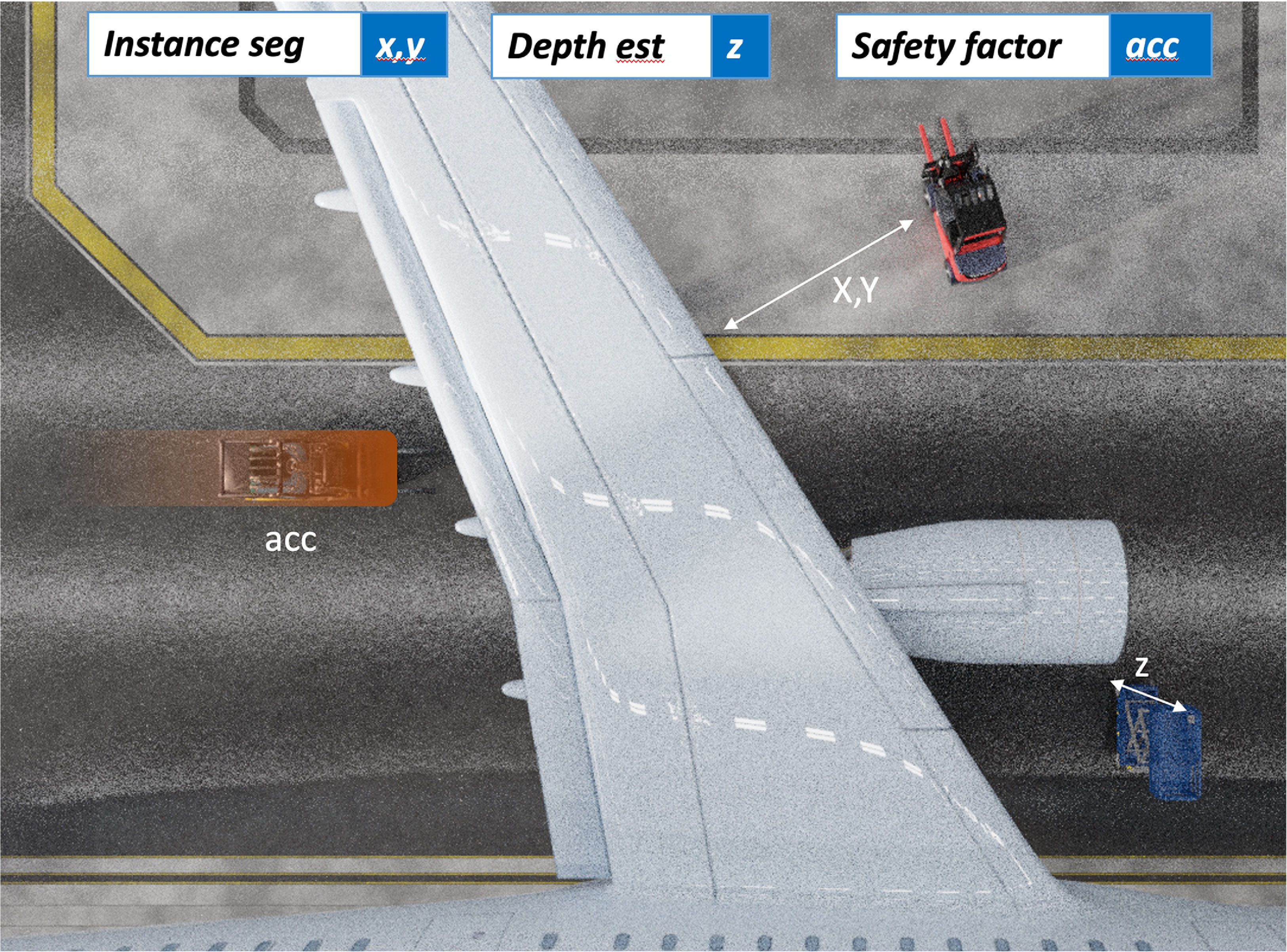
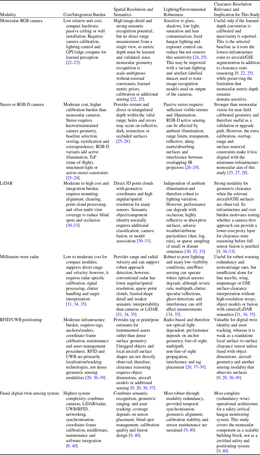
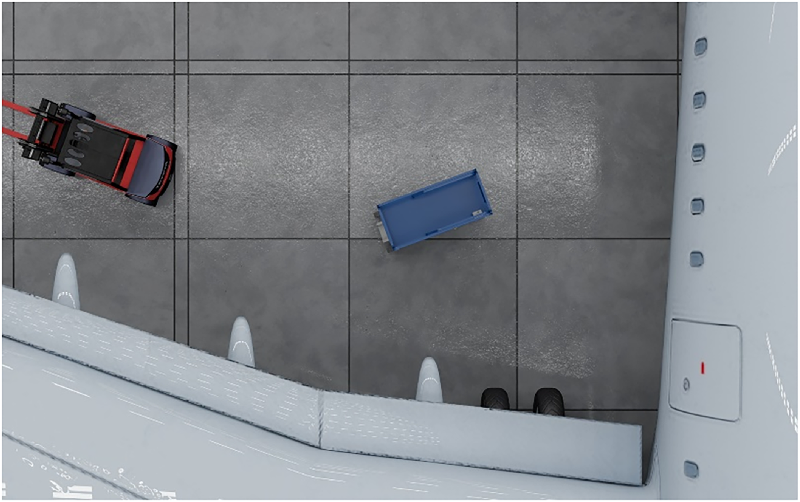
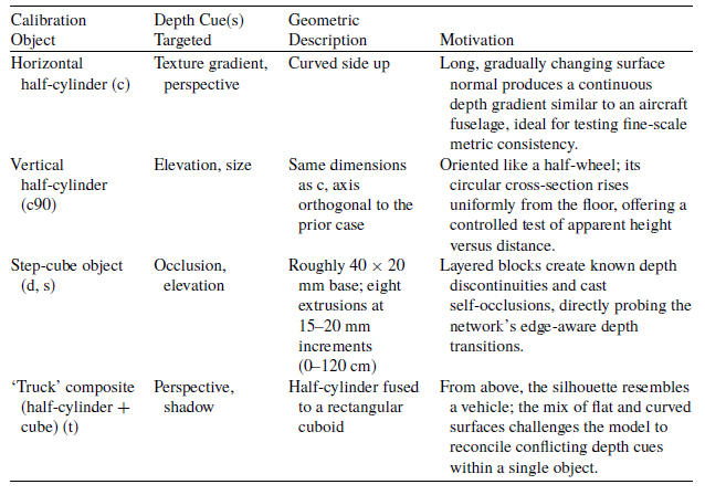
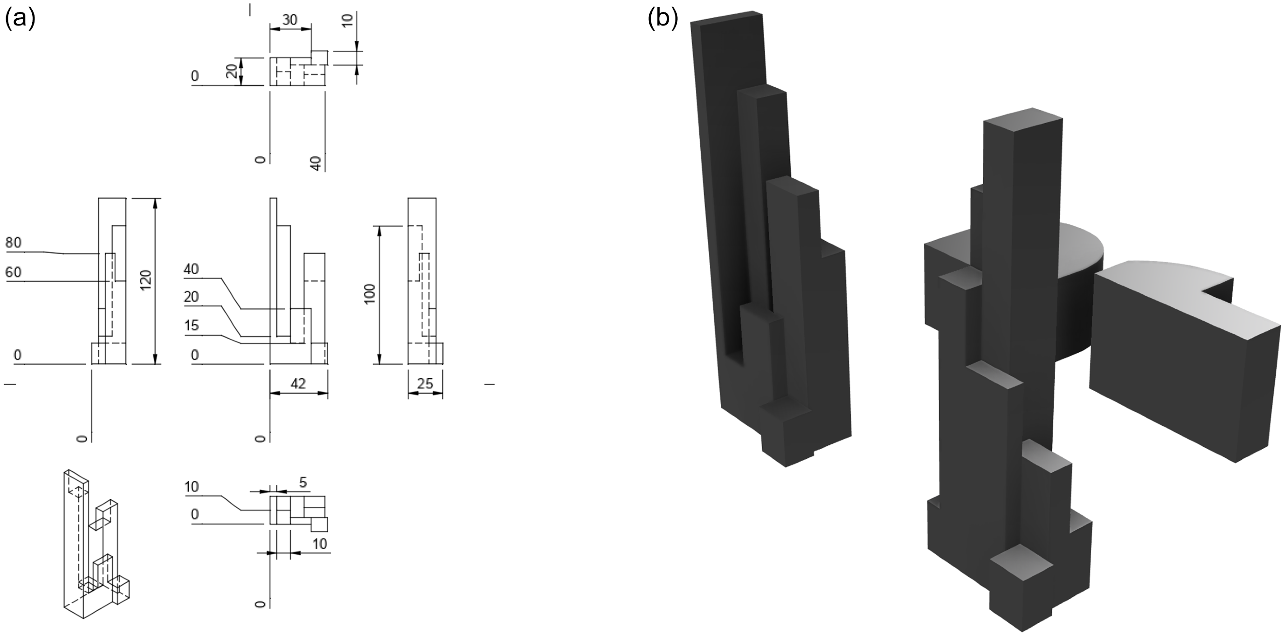
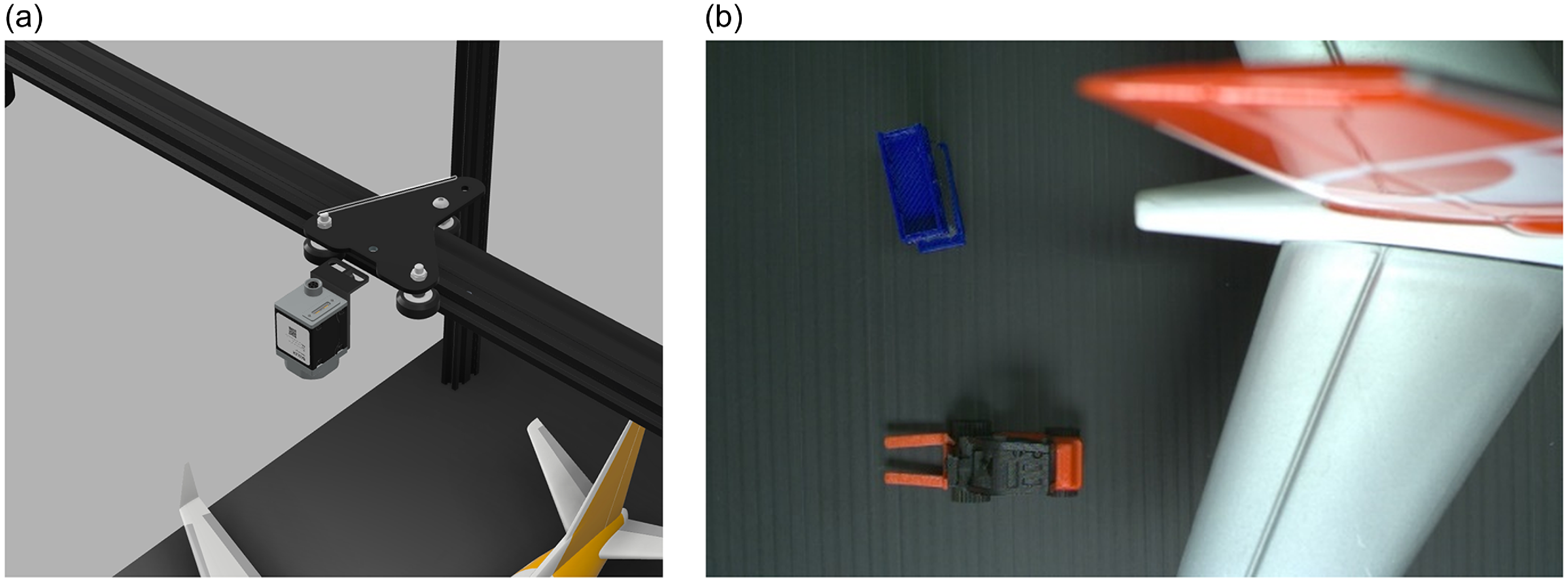
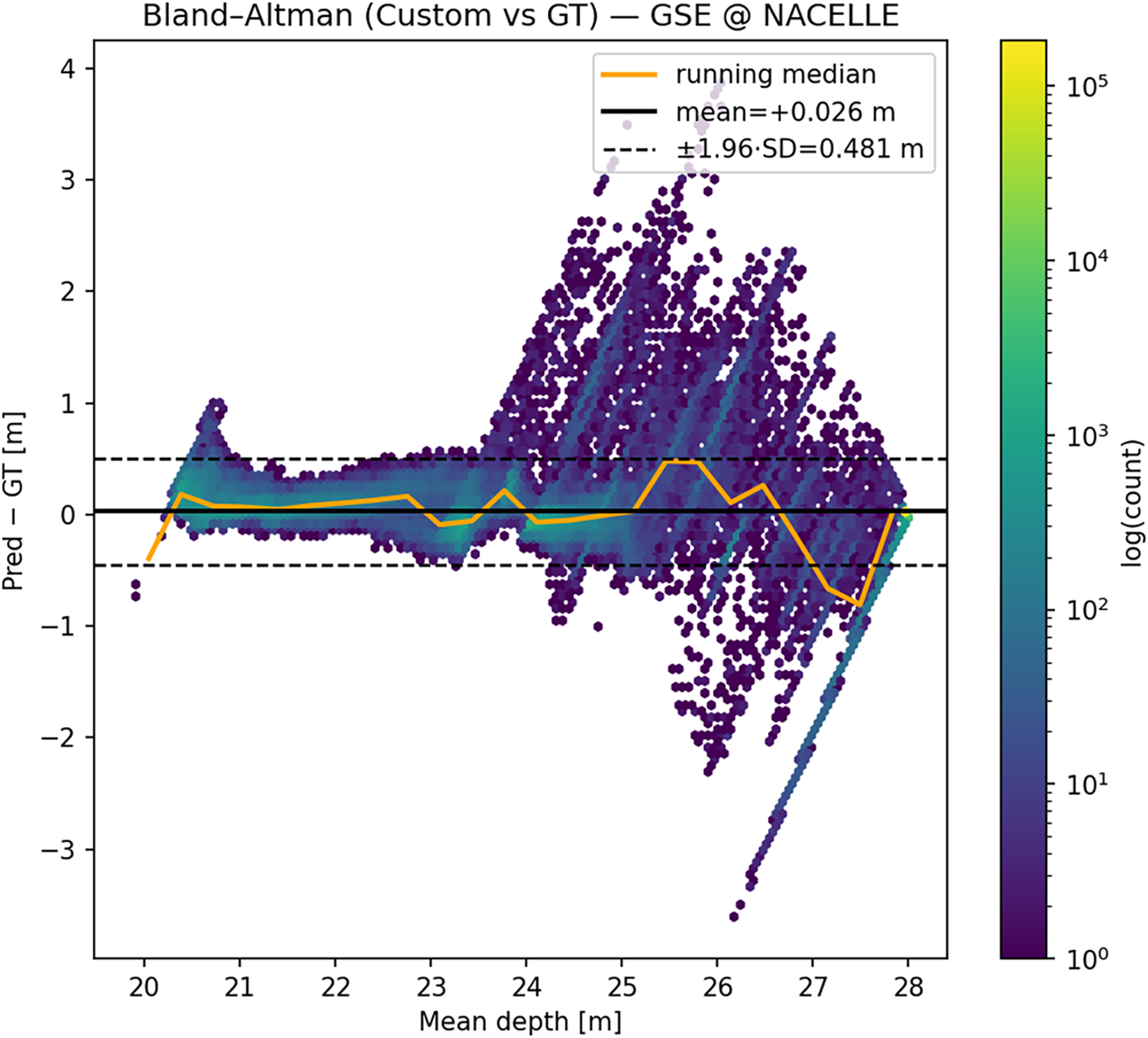
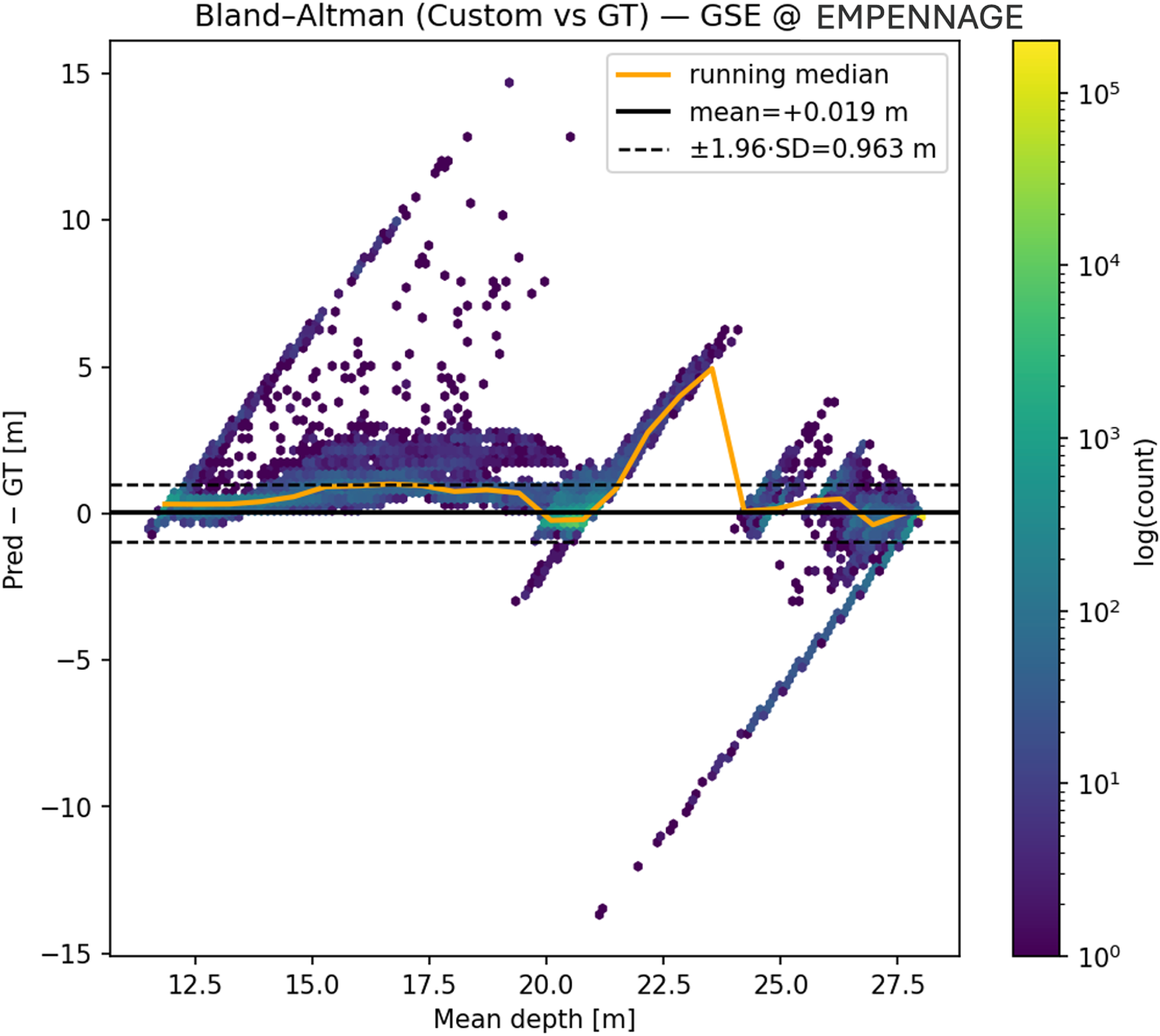
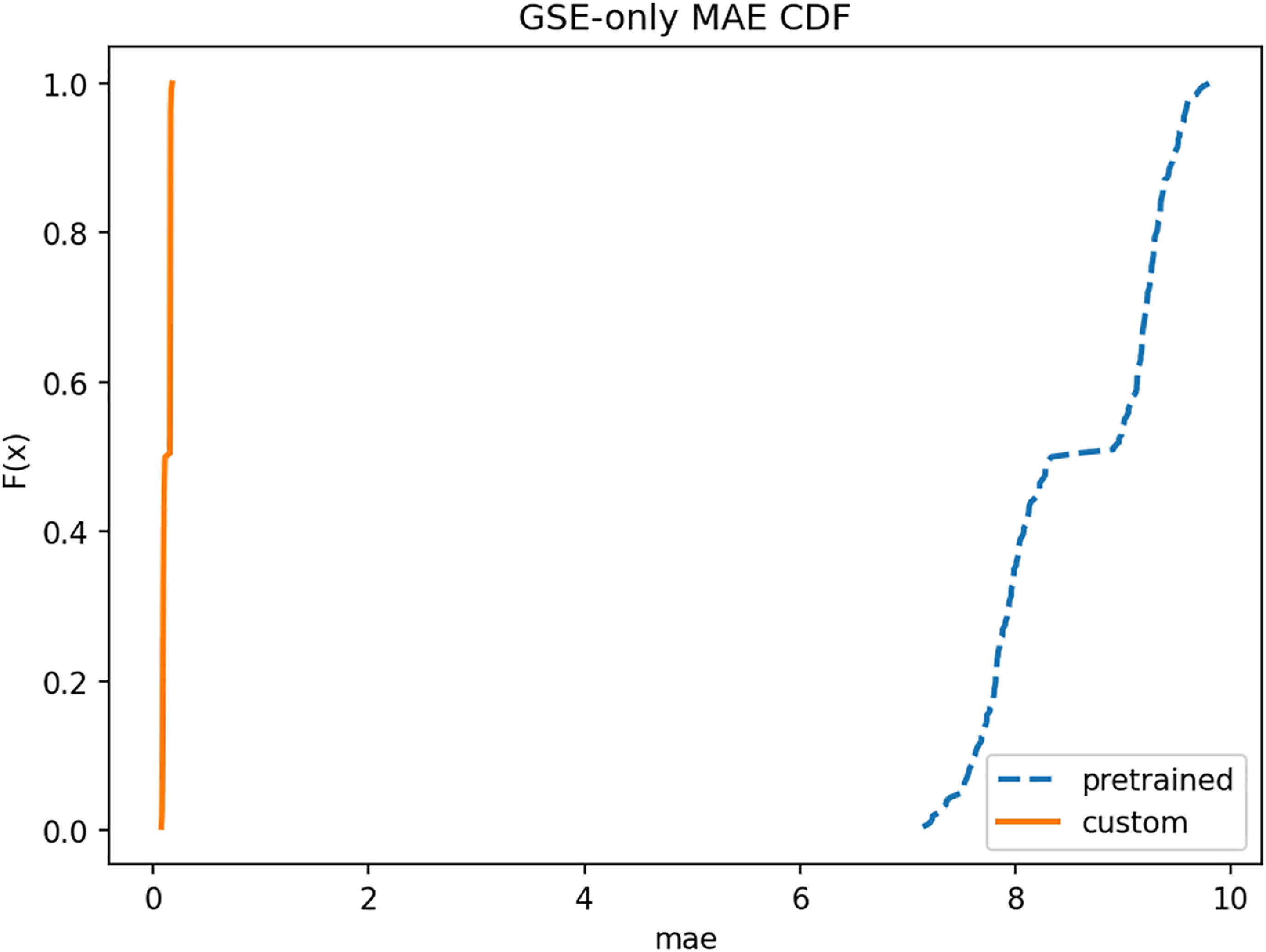
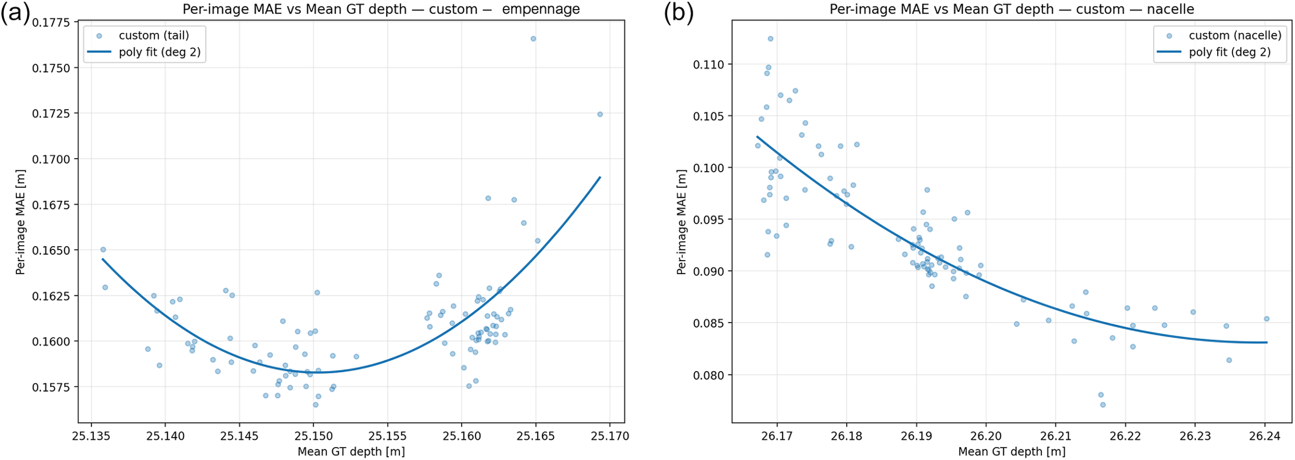
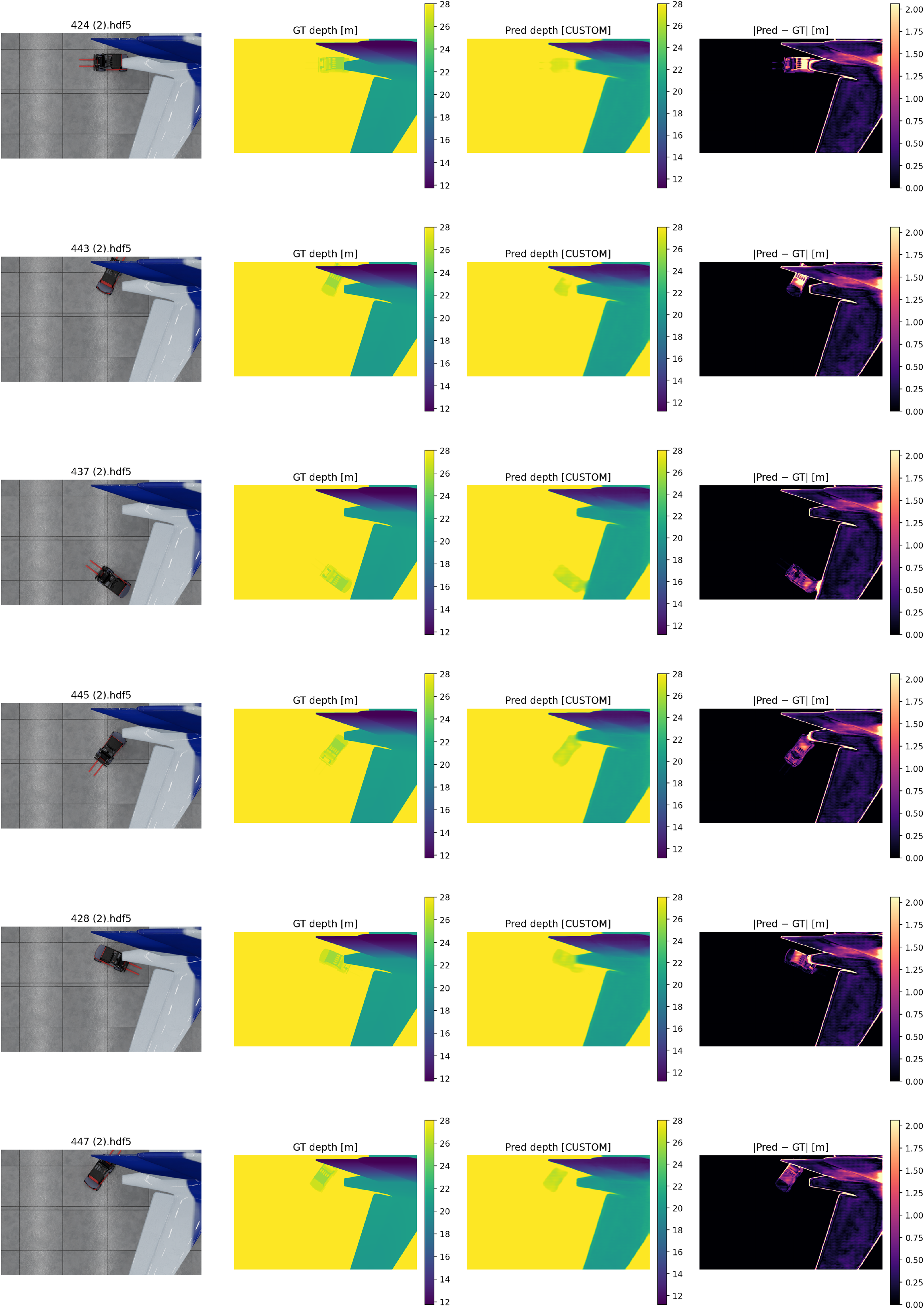
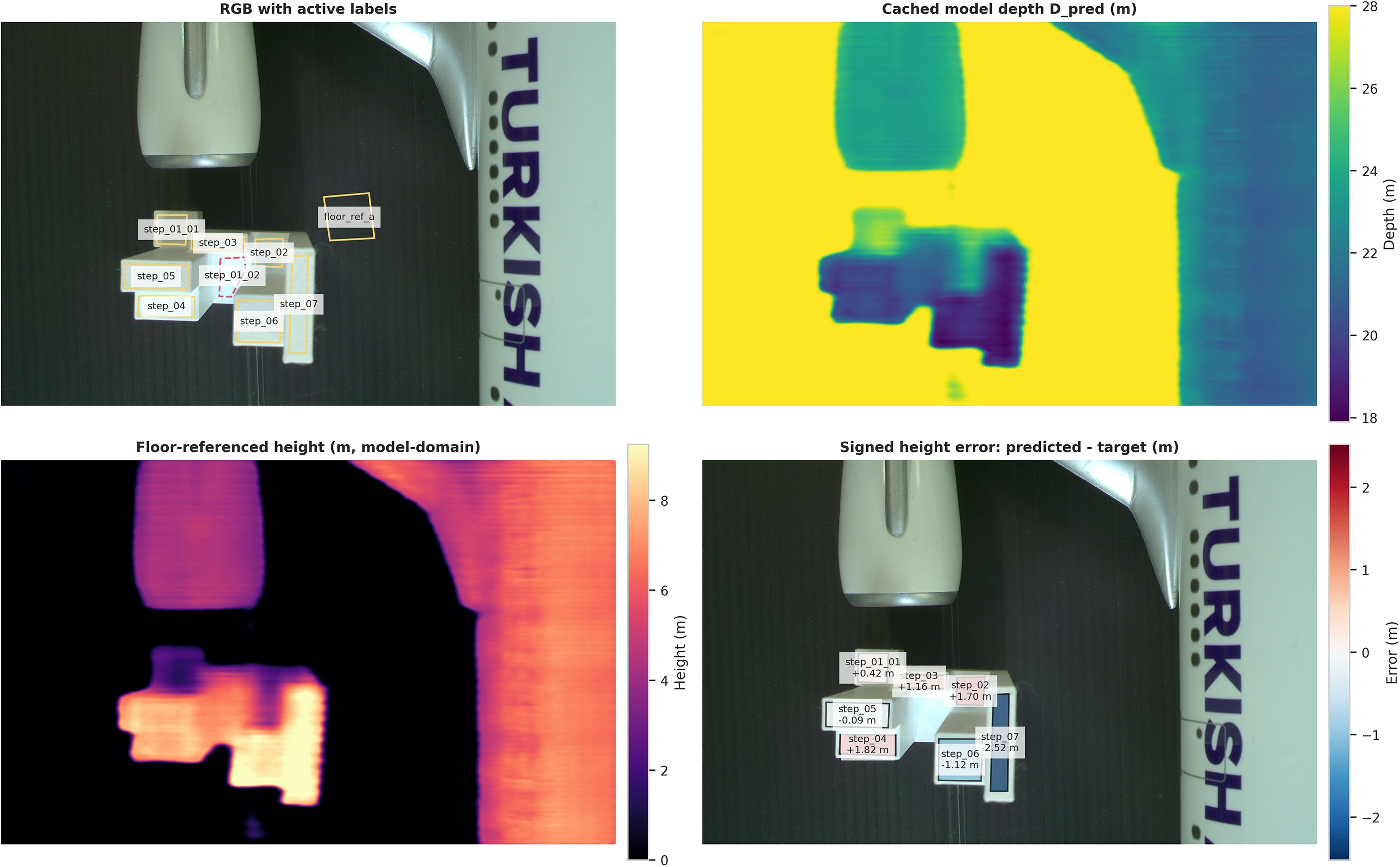
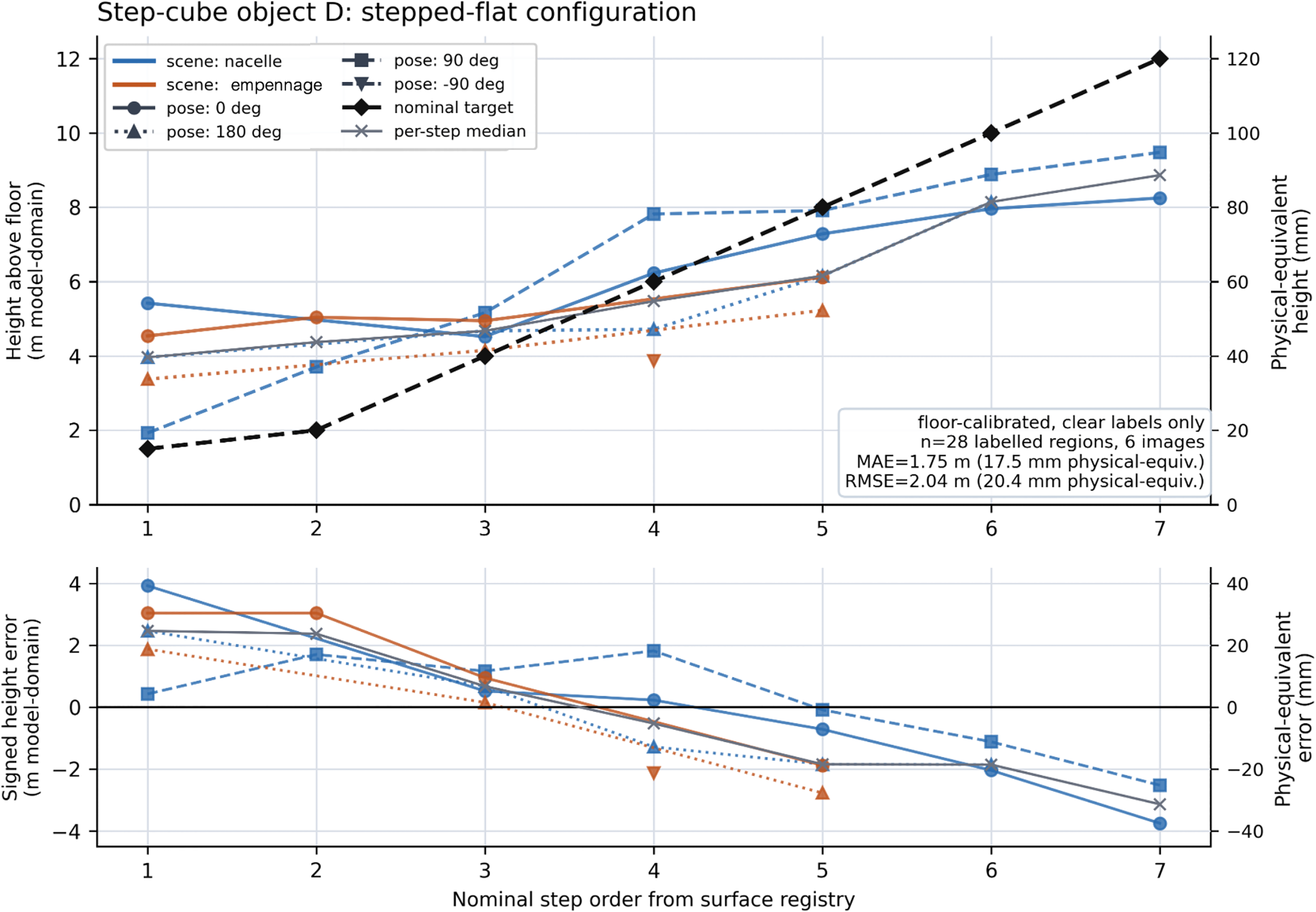
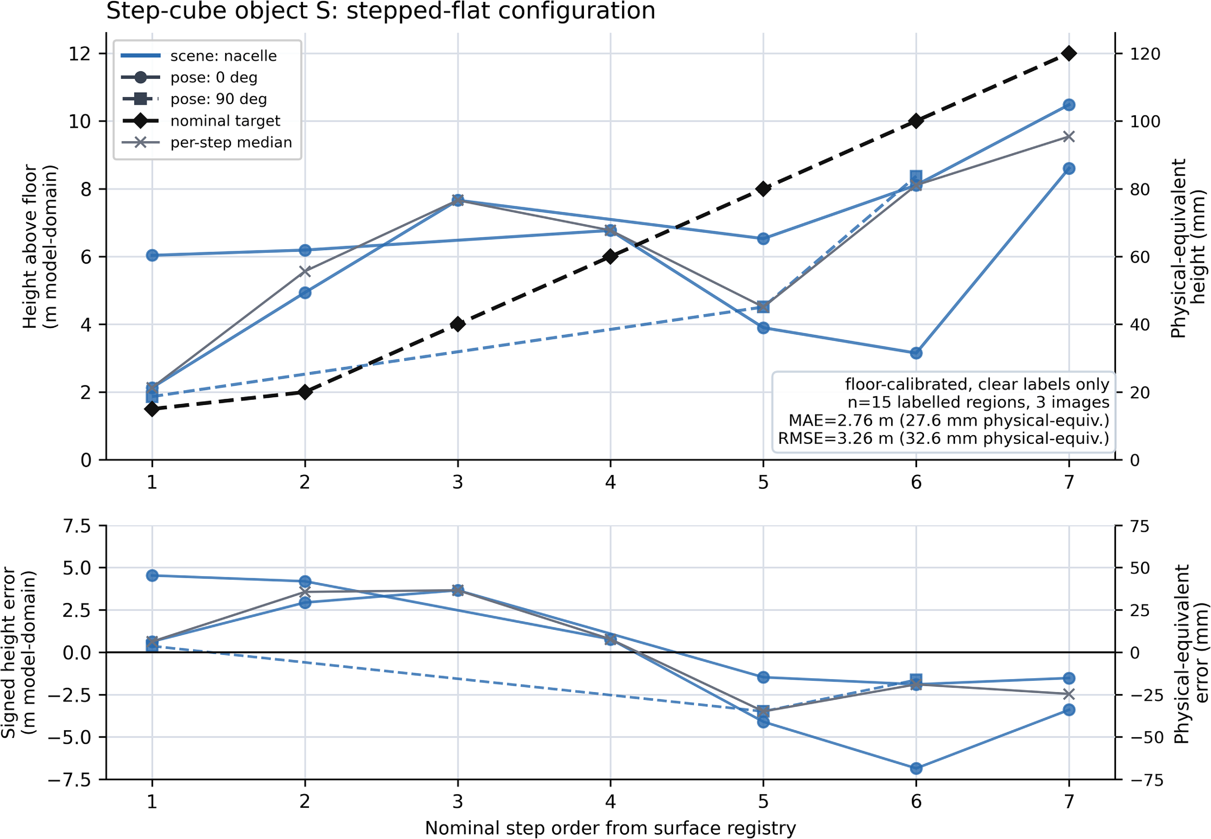
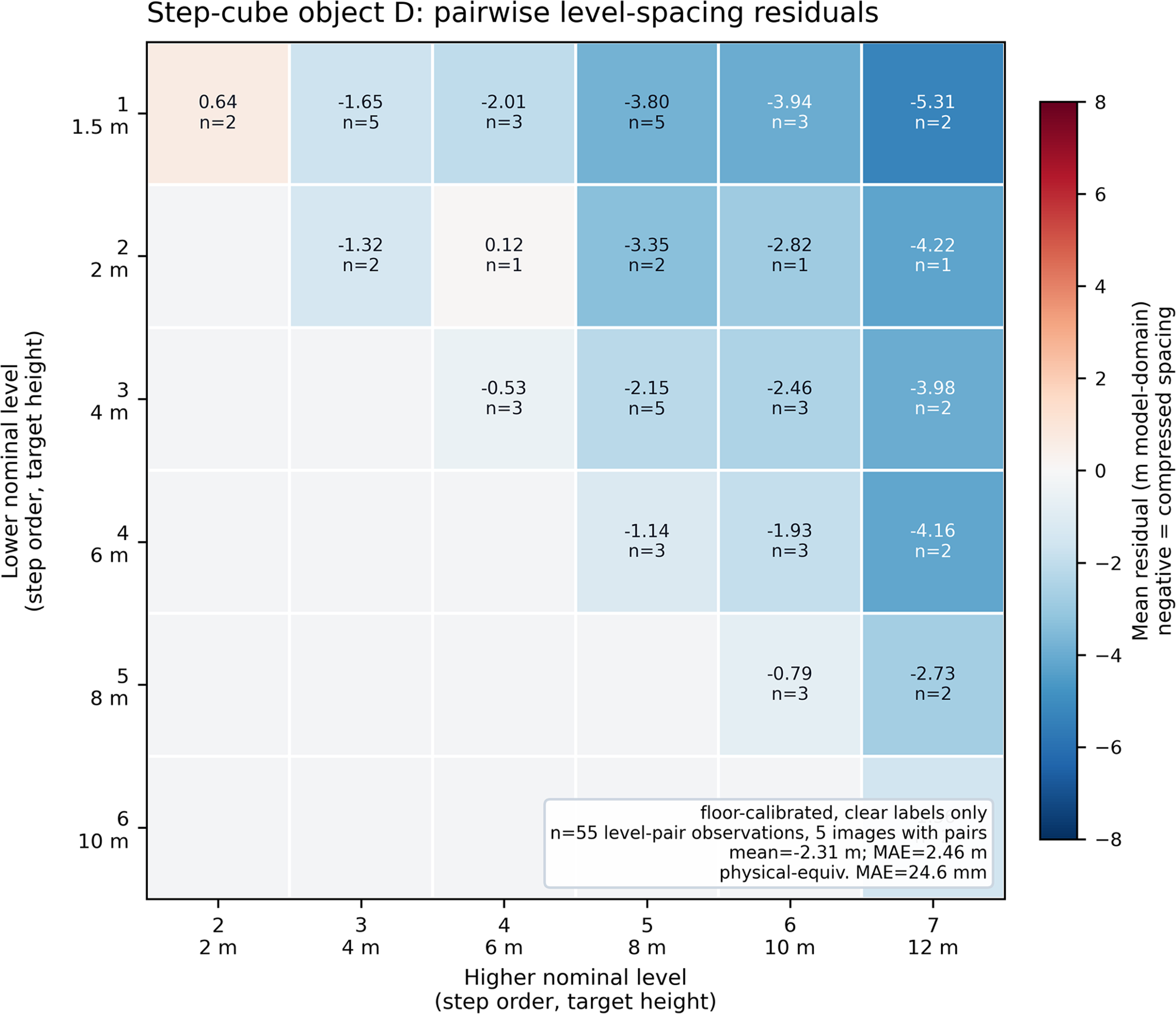
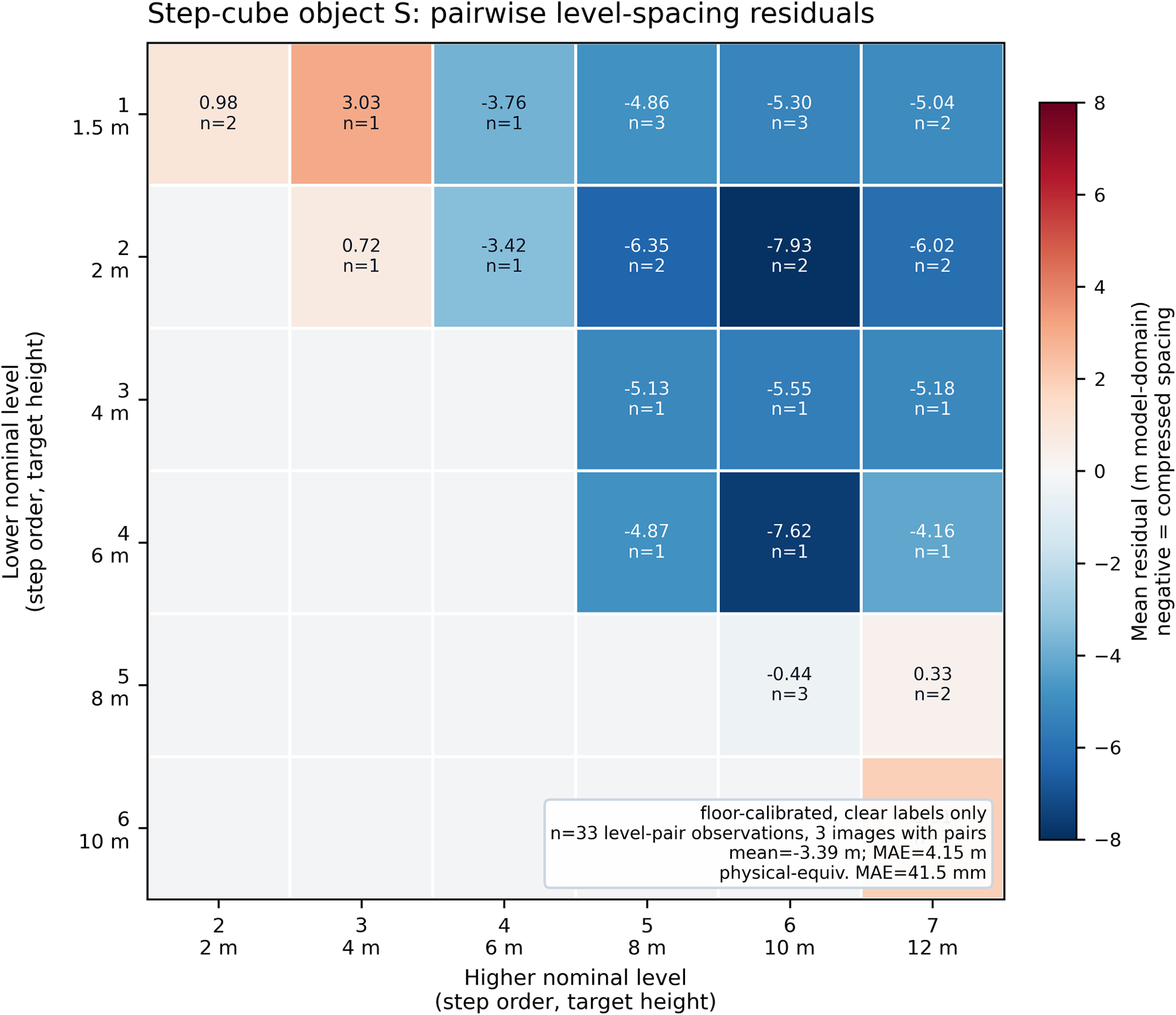
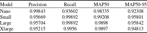
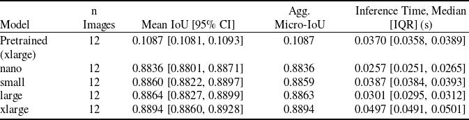
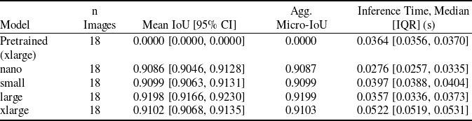
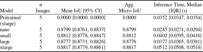
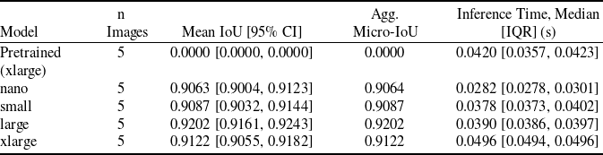
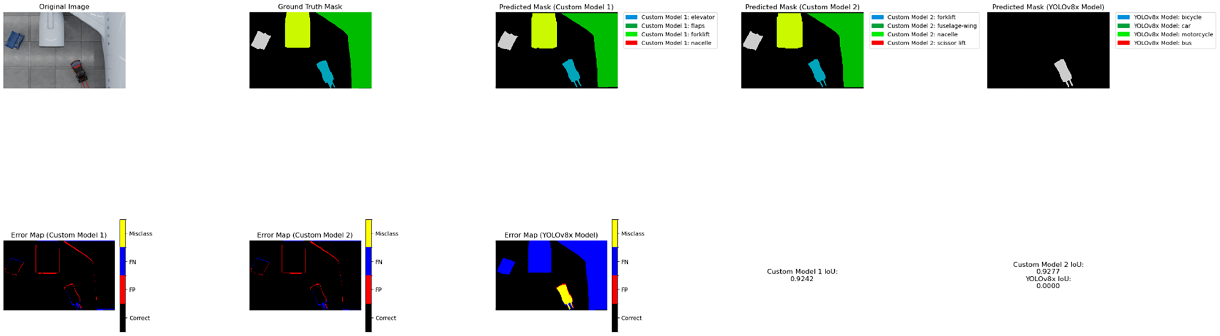
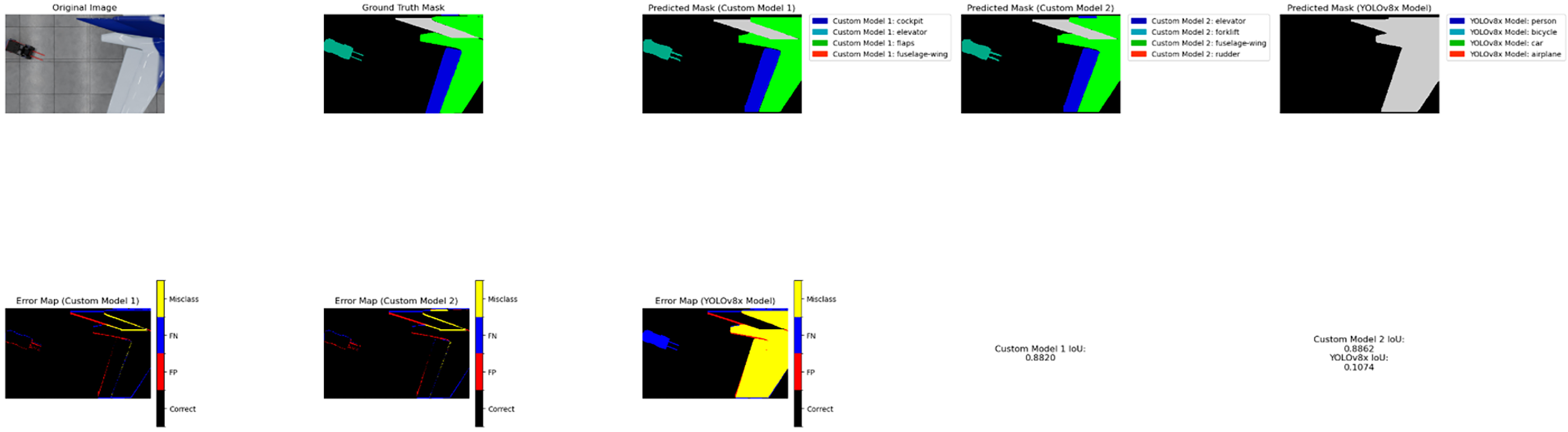
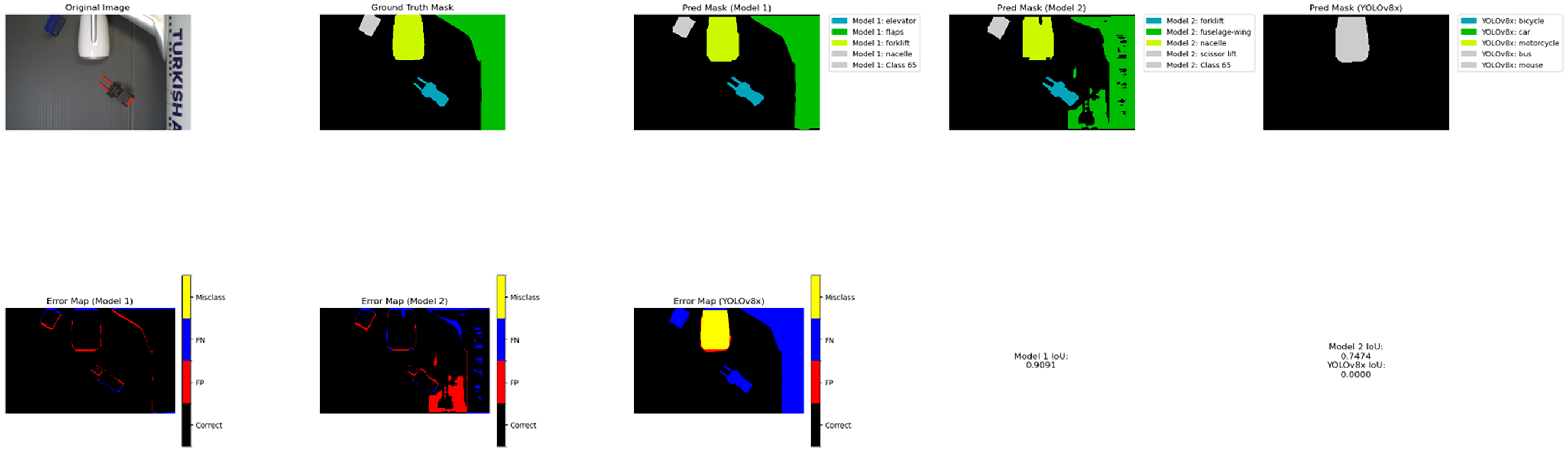
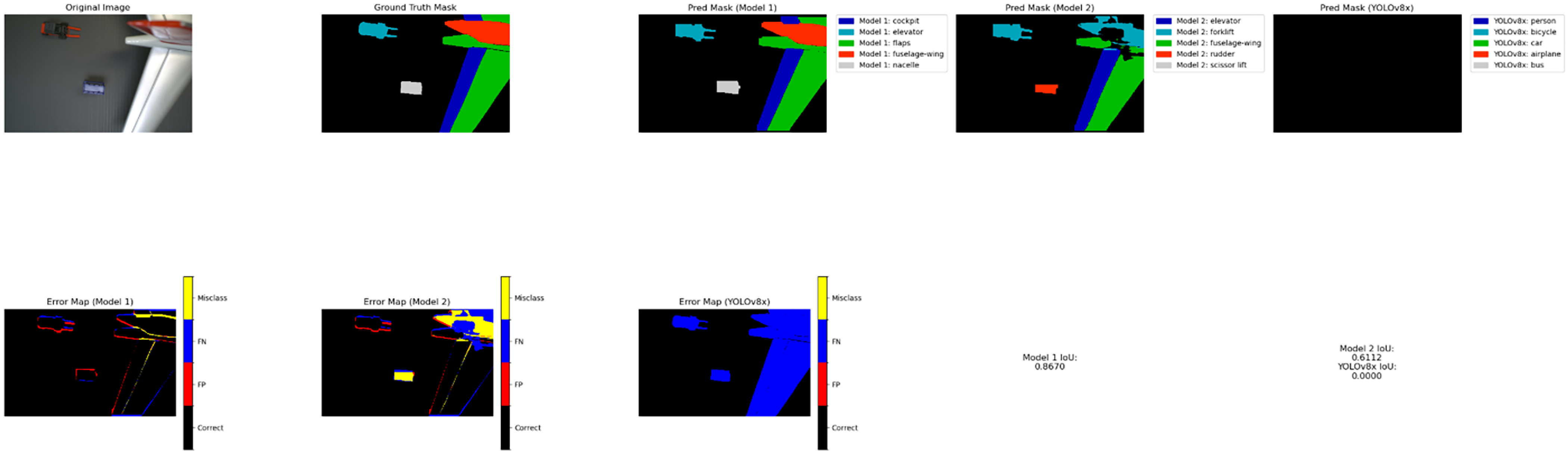
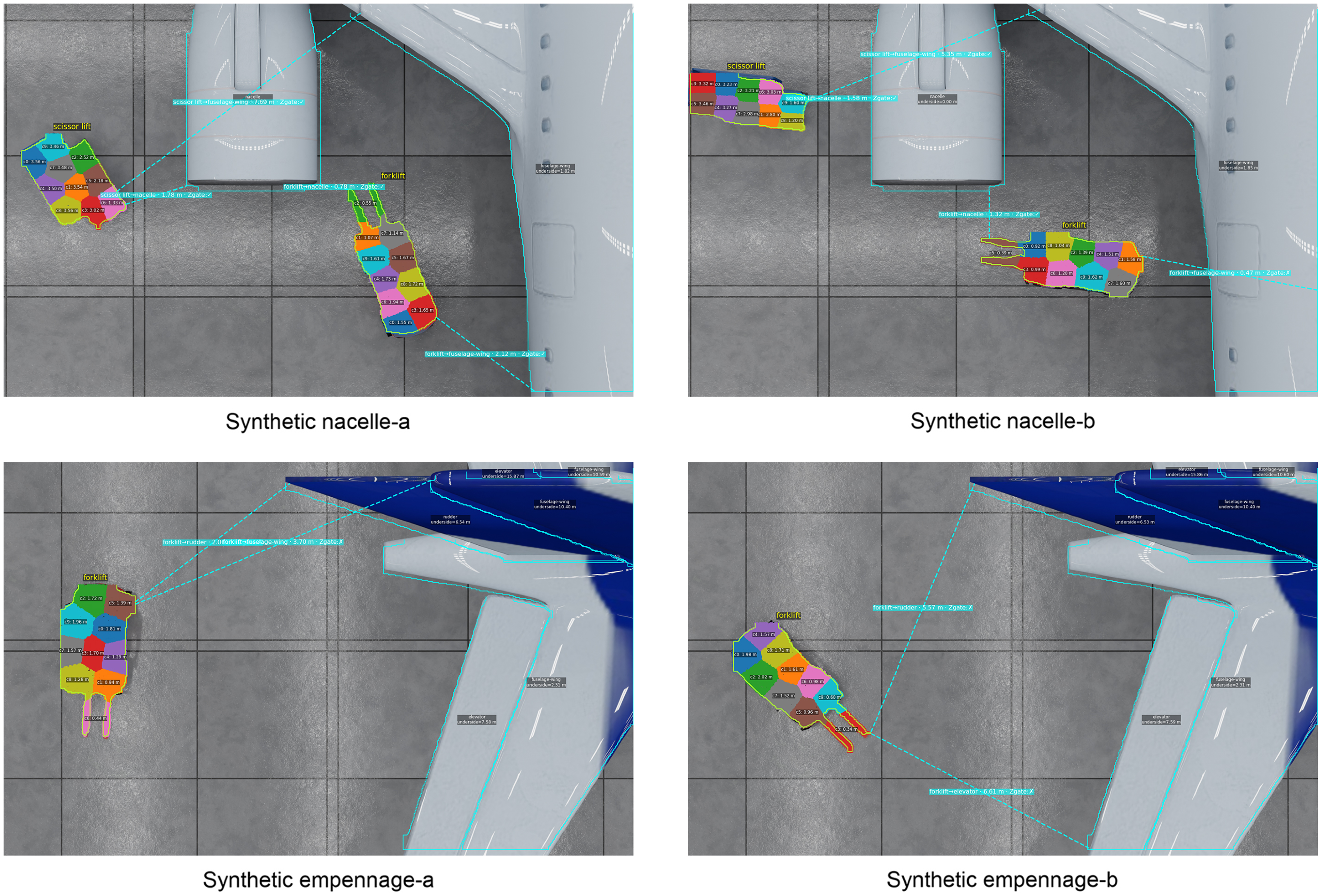
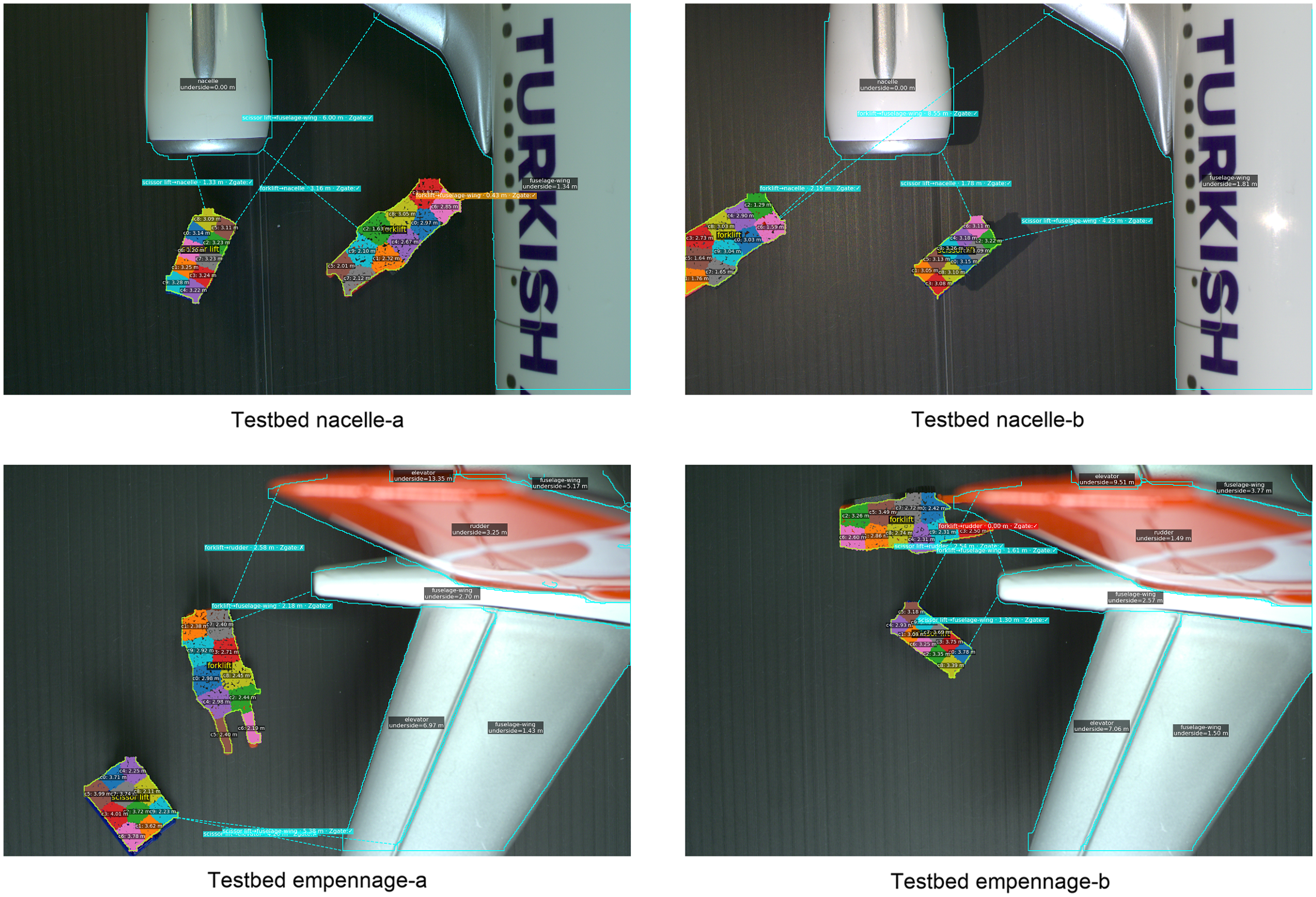

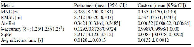

 Open access

