
1. Introduction
The system of a free flow over a porous medium region appears in a wide range of industrial and environmental applications, such as catalytic reactors, heat exchangers, fuel cells and porous river beds (Nepf Reference Nepf2012; Bottaro Reference Bottaro2019; Terzis et al. Reference Terzis, Zarikos, Weishaupt, Yang, Chu, Helmig and Weigand2019). The flow and transport processes involved are characterised by complex interactions between the porous medium and the free flow, including the two-way exchange of mass, momentum and energy across the interface (Breugem, Boersma & Uittenbogaard Reference Breugem, Boersma and Uittenbogaard2006; Manes, Poggi & Ridolfi Reference Manes, Poggi and Ridolfi2011; Fang et al. Reference Fang, Xu, He and Dey2018; Kim et al. Reference Kim, Blois, Best and Christensen2020; Suga, Okazaki & Kuwata Reference Suga, Okazaki and Kuwata2020). Understanding the transport behaviour at the permeable interface is a non-trivial challenge, which involves a wide range of properties of the porous medium, such as permeability (Suga, Nakagawa & Kaneda Reference Suga, Nakagawa and Kaneda2017; Voermans, Ghisalberti & Ivey Reference Voermans, Ghisalberti and Ivey2017; Rosti, Brandt & Pinelli Reference Rosti, Brandt and Pinelli2018), surface roughness (Kim et al. Reference Kim, Blois, Best and Christensen2020) and pore geometry (Suga et al. Reference Suga, Okazaki and Kuwata2020; Shen, Yuan & Phanikumar Reference Shen, Yuan and Phanikumar2020; McCorquodale & Munro Reference McCorquodale and Munro2021; Xu et al. Reference Xu, Altland, Yang and Kunz2021). The early works have (Finnigan Reference Finnigan2000; Jiménez et al. Reference Jiménez, Uhlmann, Pinelli and Kawahara2001; Breugem et al. Reference Breugem, Boersma and Uittenbogaard2006) established a framework for the coupling dynamics across the interface, which can be summarized as competing mechanisms in the flow: the formation of wall-attached eddies and the disruption by shear layer instabilities. When the permeability is low, the near-wall structures are less disrupted and behave as the canonical wall-bounded flow. However, as the permeability increases, large-scale vortical structures related to Kelvin–Helmholtz (KH) type instabilities emerge in the surface flow. Meanwhile, the characteristics of the near-wall cycle are substantially weakened. This scenario is supported by both experimental (Kim et al. Reference Kim, Blois, Best and Christensen2018) and numerical results (Manes et al. Reference Manes, Pokrajac, McEwan and Nikora2009; Kuwata & Suga Reference Kuwata and Suga2016; Motlagh & Taghizadeh Reference Motlagh and Taghizadeh2016; Chu et al. Reference Chu, Wang, Yang, Terzis, Helmig and Weigand2021).
Apart from the traditional isotropic porous medium, attention has recently been drawn to the anisotropic permeability. Rosti, Cortelezzi & Quadrio (Reference Rosti, Cortelezzi and Quadrio2015); Rosti et al. (Reference Rosti, Brandt and Pinelli2018) conducted a parameter study with direct numerical simulation (DNS). They found that the total drag over a permeable wall could be reduced by approximately 20 % by adjusting the diagonal components of the permeability towards streamwise and spanwise directions. Abderrahaman-Elena & García-Mayoral (Reference Abderrahaman-Elena and García-Mayoral2017); Gómez-de Segura & García-Mayoral (Reference Gómez-de Segura and García-Mayoral2019) confirmed the result of Rosti et al. (Reference Rosti, Brandt and Pinelli2018) by showing the drag reduction ability of anisotropic permeable substrates. Kuwata & Suga (Reference Kuwata and Suga2017); Suga et al. (Reference Suga, Okazaki and Kuwata2020) investigated the influence of an anisotropic permeability tensor of porous media at a higher permeable regime. It was found that streamwise and spanwise permeabilities enhance turbulence, whilst vertical permeability itself does not. In particular, the enhancement of turbulence is remarkable over porous walls with streamwise permeability, as it allows the development of streamwise large-scale perturbations induced by KH instability.
The surface roughness of porous media, in addition to permeability, also has an impact on interfacial flow. Yuan & Aghaei Jouybari (Reference Yuan and Aghaei Jouybari2018) compared turbulence statistics of turbulent open-channel flows over a smooth wall and wall roughness with different textures. They showed that the shear production peaks near the roughness crest while the individual form-induced productions are more texture sensitive and peak at a lower elevation. Kim et al. (Reference Kim, Blois, Best and Christensen2020) investigated the spatiotemporal signatures of amplitude modulation using a correlation map and a conditional averaging method. It was found that the porous media with rough surfaces are subject to stronger penetration of the flow into the permeable bed modulated by large-scale structures in the surface flow. Wang et al. (Reference Wang, Yang, Evrim, Terzis, Helmig and Chu2021c) reveal the dependence of turbulent transport on the slope angle formed by the top-layer cylinders using the conditional average.
Despite the latest advancements in the field, the interfacial transport process is far from being completely understood. In particular, the fundamental cause-and-effect relations between the surface and subsurface flows are not systematically inspected. In many cases, a causal relationship between flow quantities is inferred using linear correlation (Breugem et al. Reference Breugem, Boersma and Uittenbogaard2006; Kim et al. Reference Kim, Blois, Best and Christensen2020; Chu et al. Reference Chu, Wang, Yang, Terzis, Helmig and Weigand2021; Wang, Pan & Wang Reference Wang, Pan and Wang2021b), which is closely related to the linear stochastic estimation (LSE) introduced by Adrian & Moin (Reference Adrian and Moin1988). Recently, nonlinear modelling of dynamics based on the neural network has also found popularity in the fluid mechanics community. For example, Srinivasan et al. (Reference Srinivasan, Guastoni, Azizpour, Schlatter and Vinuesa2019) assessed the capabilities of neural networks to predict temporally evolving turbulent flows with two types of neural networks: the multilayer perceptron and the long short-term memory networks. Kim & Lee (Reference Kim and Lee2020) used convolutional neural networks (CNN) to predict the wall-normal heat flux in a turbulent channel flow with nearby wall shear stresses and pressure fluctuations. Guastoni et al. (Reference Guastoni, Guemes, Ianiro, Discetti, Schlatter, Azizpour and Vinuesa2021) predict heat flux at the wall by taking the orthogonal basis functions of wall shear stress and pressure obtained through proper orthogonal decomposition (POD) as the input of CNN. However, for both the linear and nonlinear methods mentioned above, the causal relationship between the input and output data is largely presumed, and the optimization of the inputs can only be achieved by a posteriori analysis of the model performance. This limits their ability to make causal inferences.
Two decades ago, the concept of transfer entropy was proposed by Schreiber (Reference Schreiber2000) as a tool to evaluate the directional information transfer between a source signal and a target signal. Schreiber (Reference Schreiber2000)'s definition of transfer entropy measures the information contained in the source about the next state of the target that was not already contained in the target's past. This allows one to differentiate the direction of the information flux, and can therefore be used to quantify causal interactions. Recently, Lozano-Durán (Lozano-Durán, Bae & Encinar Reference Lozano-Durán, Bae and Encinar2020; Lozano-Durán et al. Reference Lozano-Durán, Constantinou, Nikolaidis and Karp2021) highlighted the importance of causal inference in fluid mechanics and proposed leveraging information-theoretic metrics to explore causality in turbulent flows. Lozano-Durán & Arranz (Reference Lozano-Durán and Arranz2022) revisited the definition of information flux and derived a new definition of causality, which is grounded on the conservation of information in the dynamics of a system. The new definition takes into account the intermediate variables, which Schreiber's definition does not. The settings of time lags and normalization are also optimized to achieve conservation of information. Wang et al. (Reference Wang, Chu, Lozano-Durán, Helmig and Weigand2021a) used transfer entropy as a marker to evaluate the causal interaction between turbulent channel flow and porous media consisting of circular cylinders. The POD time coefficients of the leading-order modes were extracted as the representative signals for surface and subsurface flow. The result showed that top-down and bottom-up interactions are strongly asymmetric for low permeability cases, the former being mostly influenced by small near-wall eddies. As the porosity increases, both top-down and bottom-up interactions are dominated by shear-flow instabilities.
The explorations above illustrate the potential strength of information-theoretic tools in revealing the surface/subsurface coupling dynamics. However, there are still numerous challenges and unanswered questions. In the work of Wang et al. (Reference Wang, Chu, Lozano-Durán, Helmig and Weigand2021a), the source and target signals are selected as the time coefficients of the orthogonal basis of the flow fields. For the leading-order modes investigated, the spatial location is fixed for each pore unit, and the scale of flow motions are constrained to a relatively large-scale range. Therefore, the dependence of transfer entropy on spatial location and spectral components is not fully explored. In addition, transfer entropy is a purely statistical concept, which is difficult to associate with a certain type of flow motion. It is also quite challenging to testify whether the abstract conclusion derived from transfer entropy is solid. In the current work, we will compute spatial and spectral-resolved transfer entropy between turbulent fluctuations in channel flows over porous media. We use the local transfer entropy as a marker and determine which flow events in the boundary layer and the porous domain exhibit the most significant information flux. In addition, we leverage artificial neural networks as a practical model to validate the statistical results of transfer entropy. The work is organized as follows. In § 2 we present the numerical details of the DNS dataset. In § 3 coupling dynamics will be inspected in detail using spatial and spectral-resolved transfer entropy, including validation by a neural network model. Finally, conclusions are offered in § 4.
2. Numerical set-up
In our DNS the three-dimensional incompressible Navier–Stokes equations are solved in non-dimensional form,
 \begin{gather} \frac{\partial u_j}{\partial x_j}=0, \end{gather}
 \begin{gather} \frac{\partial u_i}{\partial t}+\frac{\partial u_i u_j}{\partial x_j}={-}\frac{\partial p}{\partial x_i}+\frac{1}{Re_D}\frac{\partial^2 u_j} {\partial x_i \partial x_j}+\varPi \delta_{i1}, \end{gather}
where  $\varPi$ is a constant pressure gradient in the mean-flow direction. The governing equations are normalized using the half-width of the whole simulation domain
 $H$ (figure 1a) and the averaged bulk velocity
 $U_b$ of the channel region (
 $y/H=[0,1]$). Hereafter, the velocity components in the streamwise
 $x$, wall-normal
 $y$ and spanwise
 $z$ directions are denoted as
 $u$,
 $v$ and
 $w$, respectively. The domain size (
 $L_x/H \times L_y/H \times L_z/H$) is
 $10 \times 2 \times 0.8{\rm \pi}$ in all cases. The lower half (
 $y/H=[-1,0]$) contains the porous media, and the upper half (
 $y/H=[0,1]$) is the channel flow. The porous layer consists of 50 cylinder elements along the streamwise direction and five rows in the wall-normal direction, as illustrated in figure 1. The distance
 $D$ between two nearby cylinders is fixed at
 $D/H=0.2$. A no-slip boundary condition is applied to the cylinders, the upper wall and the lower wall. Periodic boundary conditions are used in both streamwise and spanwise directions.
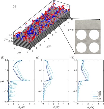
(a) Configuration of the computational domain (C05), the permeability in three directions can be found in table 1. The blue and red isosurfaces show the wall-normal fluctuation  $v'/u^p_\tau$ at level
 $-0.4$ and
 $0.4$, respectively. Panels (b–d) show the profiles of the streamwise
 $u'$, wall-normal
 $v'$ and spanwise
 $w'$ fluctuation intensity, respectively.

Simulation parameters. The porosity of the porous medium region is  $\varphi$. The friction Reynolds numbers are
 $Re_{\tau }^{p}$ and
 $Re_{\tau }^{s}$ for the porous and impermeable top walls, respectively. Here
 $\sqrt {K_{\alpha \alpha }}^{p+}$ and
 $C_{\alpha \alpha }^{{p+}}$ are the diagonal components of the permeability tensor and Forchheimer coefficient, respectively, in the direction of
 $\alpha$ (
 $\alpha \in \{x, y,z \}$), which are normalized by wall units;
 $r_c^{{p+}}$ is the radius of the cylinders.

The spectral/ $hp$ element solver Nektar++ is used to solve ((2.1) and (2.2)) (Cantwell et al. Reference Cantwell, Sherwin, Kirby and Kelly2011; Chu et al. Reference Chu, Yang, Pandey and Weigand2019, Reference Chu, Wu, Rist and Weigand2020; Pandey et al. Reference Pandey, Chu, Weigand, Laurien and Schumacher2020). The geometry in the
 $x$–
 $y$ plane is discretized into quadrilateral elements with local refinement near the cylinders (see figure 1a). Local element expansions are applied based on the modified Legendre basis (Karniadakis, Karniadakis & Sherwin Reference Karniadakis, Karniadakis and Sherwin2005). We used flexible polynomial orders across the wall-normal range in a continuous Galerkin projection. The polynomial order in the free flow region
 $y/H=[0.2, 1]$ is
 $P=6\unicode{x2013}7$. The near-wall region and the top two layers of cylinders
 $y/H=[-0.4, 0.2]$ are enhanced with a higher order of
 $P=8\unicode{x2013}9$. A lower order of
 $P=5$ is selected in the deeper positions of the cylinder array (
 $y/H=[-1, -0.4]$). The spanwise direction is extended with a Fourier spectral method. The 2/3 rule is used to avoid aliasing errors. The time stepping is performed with a second-order mixed implicit–explicit scheme proposed by Karniadakis, Israeli & Orszag (Reference Karniadakis, Israeli and Orszag1991). The time step is fixed at
 $\Delta T/(H/U_b)=5\times 10^{-4}$.
Four DNS cases are performed with varying porosity  $\varphi =0.5,0.6,0.7$ and
 $0.8$, which is defined as the ratio of the void volume to the total volume of the porous structure. The parameters of the simulated cases are listed in table 1, where the cases are named after their respective porosity. The superscripts
 $(\,\cdot\,)^p$ and
 $(\,\cdot\,)^{s}$ represent permeable wall and smooth wall side variables, respectively. Variables with superscript
 $^+$ are scaled by friction velocities
 $u_\tau$ of their respective side and viscosity
 $\nu$.
For an arbitrary variable  $\phi$, we denote the time-averaged value as
 $\bar {{\cdot }}$, i.e.
 $\bar {\phi }=1/T\int _{0}^{\rm T}\phi \,\mathrm {d}t$, and spatial-averaged value in the
 $x$–
 $z$ plane as
 $\langle \,\cdot \,\rangle$, i.e.
 $\langle \phi \rangle =1/A_f \int _{A_f}\phi \,\mathrm {d}A$,
 $A_f$ being the fluid area. The instantaneous turbulent fluctuation is
 $\phi '=\phi -\bar {\phi }$, and the form-induced fluctuation is
 $\tilde {\bar {\phi }}=\bar {\phi }-\langle \bar {\phi } \rangle$. For the permeable wall side, the total shear stress at the interface can be derived as (Shen et al. Reference Shen, Yuan and Phanikumar2020; Suga et al. Reference Suga, Okazaki and Kuwata2020)
 \begin{equation} \tau_{w}^p= \left ( \mu \frac{\partial \langle \bar{u} \rangle}{\partial y} - \rho\langle\overline{u^{\prime}v^{\prime}}\rangle -\rho\langle{ \tilde{\bar{u}} \tilde{\bar{v}}}\rangle\right )_{y=0}. \end{equation}
For the smooth wall side, the total shear stress is
 \begin{equation} \tau_{w}^s= \left ( \mu \frac{\partial \langle \bar{u} \rangle}{\partial y}\right )_{y=H}. \end{equation}
The friction velocity can then be calculated from total shear stress at both walls, i.e.  $u_\tau ^p=\sqrt {\tau _w^p/\rho }$ and
 $u_\tau ^s=\sqrt {\tau _w^s/\rho }$. The friction coefficients at the permeable and smooth walls are defined as
 $C_f^p=\tau _{w}^p/(\tfrac {1}{2}\rho U_b^2)$ and
 $C_f^s=\tau _{w}^s/(\tfrac {1}{2}\rho U_b^2)$, respectively, which are listed in table 1.
Note that the distance between cylinders is fixed, and the porosity is changed by varying the radius of the cylinders. The normalized cylinder radius is in the range  $r_c^{p+}=r_c u_\tau ^{p}/\nu =42$–
 $52$ for all the cases tested (see table 1), such that the effect of surface roughness is assumed to be at a similar level. For all the cases, the Reynolds number of the top wall boundary layer is set to be
 $Re_\tau ^{s}=\delta ^{s}u_\tau ^{s}/\nu \approx 180$ (
 $\delta$ is the distance between the position of maximum streamwise velocity and the wall). In this manner, changes in the top wall boundary layer are minimized. On the top smooth wall side, the streamwise cell size ranges from
 $4.1\le \Delta x^{s+}\le 6.3$ and the spanwise cell size is below
 $\Delta z^{s+}=5.4$. On the porous media side,
 $\Delta z^{p+}$ is below 8.4, whereas
 $\Delta x^{p+}$ and
 $\Delta y^{p+}$ are enhanced by polynomial refinement of local mesh (Cantwell et al. Reference Cantwell, Sherwin, Kirby and Kelly2011). The total number of grid points ranges from 88
 $\times 10^6$ (C05) to 595
 $\times 10^6$ (C08). Each cylinder in the porous domain is resolved with 80 to 120 grids along the perimeter. The spatial resolution of the present work is close to those of previous DNS investigations. For example, Shen et al. (Reference Shen, Yuan and Phanikumar2020) conducted DNS of a turbulent flow over sediment beds using the immersed boundary method, where the diameter was discretized into 36–50 points. The mesh of Karra et al. (Reference Karra, Apte, He and Scheibe2022) had 26 grid points along the diameter of each grain. Wu, Christensen & Pantano (Reference Wu, Christensen and Pantano2020) investigated the turbulent channel flow with hemispherical roughness using the spectral element method. Each hemisphere was resolved by 50 grid points. In addition, the high-order scheme used in the current work with body-fitted mesh has a significant advantage in resolving fine scales and requires fewer grids than the finite volume method and immersed boundary method to reach the same accuracy (Kooij et al. Reference Kooij, Botchev, Frederix, Geurts, Horn, Lohse, van der Poel, Shishkina, Stevens and Verzicco2018; Theobald et al. Reference Theobald, Schäfer, Yang, Frohnapfel, Stripf, Forooghi and Stroh2021). Furthermore, we compared our grid resolutions with the Kolmogorov length scale
 $\eta =(\nu /\epsilon )^{1/4}$ at the interface. For all the cases,
 $(\Delta x/\eta )_{y=0}\leqslant 2$,
 $(\Delta y/\eta )_{y=0}\leqslant 1$,
 $(\Delta z/\eta )_{y=0}\leqslant 4.5$, which indicates that current resolution is sufficient (Moin & Mahesh Reference Moin and Mahesh1998).
By performing parameter tests on porous media and fitting the Darcy–Forchheimer equation, the permeability tensor  $K$ and Forchheimer coefficient
 $C$ may be obtained, and the details of the computation can be referred to Wang et al. (Reference Wang, Chu, Lozano-Durán, Helmig and Weigand2021a). The intensity profiles of
 $u'$,
 $v'$ and
 $w'$ are shown in figure 1(b–d), respectively. The turbulent intensity grows with porosity for both the channel and the porous medium region. In the current study, we focus on the up- and down-welling motions at the upper surface of the porous medium, which is represented by the fluctuation
 $v'$.
3. Results
3.1. Transfer entropy
In the current work, the transfer entropy (Schreiber Reference Schreiber2000) is used to evaluate the direction of coupling, i.e. the cause-effect relationship, between two time series. The transfer entropy originates from the framework of information theory, and is a specific version of the mutual information for conditional probability. Suppose we have two variables,  $X$ and
 $Y$, and the time sequences of their states are denoted by
 $X_t$ and
 $Y_t$ (
 $t=\ldots 1,2,3\ldots$). The transfer entropy between processes
 $X$ and
 $Y$ can be defined as
 \begin{equation} T_{Y\rightarrow X}(\Delta t)=H(X_t|X_{t-1})-H(X_t|{X_{t-1},Y_{t-\Delta t}}), \end{equation}
where  $X_t$ represents the current state of
 $X$ and
 $X_{t-1}$ denotes the immediate past of
 $X_t$. Here
 $Y_{t-\Delta t}$ is the history state of
 $Y$, which has a time lag
 $\Delta t$ from current
 $X_t$;
 $H(A|B)$ is the conditional Shannon entropy of the variable
 $A$ given
 $B$, which is defined as
 \begin{equation} H(A|B)={-}E\left[\log_2(p(A|B)\right]={-}E\left[\log_2\left(\frac{p(A,B)}{p(B)}\right) \right]=E[\log_2(p(B))]-E[\log_2(p(A,B))], \end{equation}
where  $p(\,\cdot\,)$ is the probability density function and
 $E[\,\cdot\,]$ denotes the expectation value. The terms in the form of
 $H(A|B)$ are conditional entropy, which denotes the amount of information in
 $A$ that is not contained in
 $B$.
In order to quantify the strength of causality, normalization is necessary to scale the magnitude of causality within  $[0,1]$ and eliminate small values caused by statistical errors. As proposed by Gourévitch & Eggermont (Reference Gourévitch and Eggermont2007), the normalized transfer entropy can be defined as
 \begin{equation} \tilde T_{Y\rightarrow X}=\frac{T_{Y\rightarrow X}-E[T_{Y_s\rightarrow X}]} {H(X_t|X_{t-1})}, \end{equation}
where  $E[T_{Y^s\rightarrow X}]$ is an estimation of the statistical bias and
 $Y_s$ is the surrogate variable of
 $Y$, which is acquired by randomly permuting
 $Y$ in time to break its causal links with
 $X$. The conditional entropy
 $H(X_t|X_{t-1})$ is the intrinsic uncertainty of
 $X$ knowing its history. Equation (3.3) thus represents the fraction of information in the target
 $X$ not explained by its past that is explained by
 $Y$ in conjunction with that past.
3.1.1. Local transfer entropy
The physical interpretation of the quantity of transfer entropy can be hard to grasp, and sometimes the outcome is confused with the more widely used correlation method. In the following, the results from both analysis tools will be presented and compared. A simple example will be presented to illustrate the strength of transfer entropy and explore the connection between information transfer and flow motions.
The definition of transfer entropy quantifies the statistical coherence between time-evolving systems in a global and averaged manner. Using (3.2), we rewrite (3.1) in the following form:
 \begin{equation} T_{Y\rightarrow X}(\Delta t)={-}E\left[\log_2\frac{p(x_t|x_{t-1})}{p(x_t|x_{t-1}, y_{t-\Delta t})}\right]. \end{equation}
Here  $x_{t}$ and
 $y_{t}$ are instantaneous measurements at time
 $t$ of processes
 $X$ and
 $Y$, respectively. We define local transfer entropy
 $\zeta$ as
 \begin{equation} \zeta_{Y \rightarrow X}(t,\Delta t)=\log _{2} \frac{p\left(x_{t} \mid x_{t-1}, y_{t-\Delta t}\right)}{p\left(x_{t} \mid x_{t-1}\right)}. \end{equation}
The transfer entropy in (3.1) is essentially the expectation value of the local transfer entropy, that is,
 \begin{equation} T_{Y \rightarrow X}=E[ \zeta_{Y \rightarrow X}(t, \Delta t)]. \end{equation}
It should be noted that the definition in (3.1) and (3.5) is a simplified form with the temporal length of the source and destination's history (or embedding dimension) being one. The definition can be expanded by taking more history states of  $X$ and
 $Y$ into account (Schreiber Reference Schreiber2000; Lizier, Prokopenko & Zomaya Reference Lizier, Prokopenko and Zomaya2012), which takes more samples to converge and is more complicated to explain. However, in the current work, we will concentrate on this most fundamental setting in order to build the groundwork for future research on higher embedding dimensions. Local transfer entropy characterizes the information transfer into each spatiotemporal point in a given system as opposed to a global average overall point, which provides important insights into the dynamics of nonlinear systems.
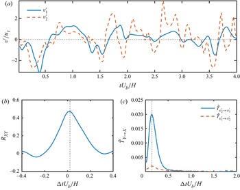
To explain the idea of (local) transfer entropy more explicitly, figure 2(a) shows the excerpts of wall-normal fluctuation  $v_1'(t)$ and
 $v_2'(t)$ of case C05, which are extracted from the middle of a first-layer cylinder gap (
 $y=-r_c$) and the crest position above the gap (
 $y=0$), respectively. The two signals
 $v_1'$ and
 $v_2'$ are acquired from the same streamwise position. Despite their clear differences in scale content, the two signals appear to be connected, with the positive and negative peaks appearing to be coordinated. This feature is also evidenced by the cross-correlation profile between
 $v_1'$ and
 $v_2'$ (see figure 2b), which is defined as
 \begin{equation} R_{vv}(\Delta t)=\overline{v_1'(t)v_2'(t+\Delta t)}/(\sigma_{v_1'}\sigma_{v_2'}), \end{equation}
where  $\Delta t$ is the shifted time interval between the two signals. The profile shows a positive peak value of 0.48 at
 $\Delta tU_b/H\approx 0.02$, revealing that the two signals are considerably correlated. However, the cross-correlation profile is generally symmetric and does not show clearly the directionality of cause and effect between signals. As a comparison, figure 2(c) shows the transfer entropy
 $\tilde T_{v_2'\rightarrow v_1'}$ and
 $\tilde T_{v_1'\rightarrow v_2'}$ as functions of
 $\Delta t$. First of all, the time delay for transfer entropy can only be positive due to the constraint that the ‘cause’ always happens before the ‘effect’. Secondly, there is a large disparity between the magnitude of
 $\tilde T_{v_2'\rightarrow v_1'}$ and
 $\tilde T_{v_1'\rightarrow v_2'}$, which reveals the strong dependence of information flux on the coupling direction. For the current signal set, the transfer entropy in both directions reaches a maximum at
 $\Delta tU_b/H\approx 0.15$. This time lag can be interpreted as the time an influence needs to propagate between the two signals, which is not necessarily the same for both coupling directions (Wibral et al. Reference Wibral, Pampu, Priesemann, Siebenhühner, Seiwert, Lindner, Lizier and Vicente2013).
Comparison between correlation and transfer entropy. (a) Excerpts of instantaneous vertical fluctuations  $v_1'$ and
 $v_2'$ at
 $y=-r_c$ (solid line) and
 $y=0$, respectively. (b) Profile of cross-correlation between
 $v_1'$ and
 $v_2'$. (c) Transfer entropy
 $\tilde T_{v_2'\rightarrow v_1'}$ (solid line) and
 $\tilde T_{v_1'\rightarrow v_2'}$ (dashed line) as a function of time delay
 $\Delta t$.

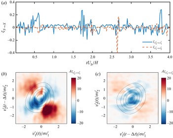
Figure 3(a) shows the local transfer entropy corresponding to the time series in figure 2(a). The time delay  $\Delta t$ is fixed at
 $\Delta tU_b/H=0.15$, corresponding to the maximum value of transfer entropy. Several observations can be made. First,
 $\zeta$ of the two transfer directions are totally different. The magnitude of
 $\zeta _{v_2'\rightarrow v_1'}$ is generally greater than that of
 $\zeta _{v_1'\rightarrow v_2'}$, which explains the disparity between the two profiles of
 $\tilde T$ in figure 2(c). Secondly, both positive and negative values exist for local transfer entropy. Unlike the global transfer entropy that is positive by definition (Schreiber Reference Schreiber2000), the value of local transfer entropy is not constrained to be larger than zero. According to the definition of local transfer entropy
 $\zeta$ (3.5), the sign of
 $\zeta$ depends on the ratio between
 $p(x_t|x_{t-1},y_{t-\delta t})$ and
 $p(x_t|x_{t-1})$. The latter represents the probability of observing
 $x_t$ given its immediate history
 $x_{t-1}$, and the former denotes the probability of observing
 $x_t$ in the condition of both
 $x_{t-1}$ and
 $y_{t-\Delta t}$. If
 $\zeta >0$, that is,
 $p(x_t|x_{t-1},y_{t-\Delta t})>p(x_t|x_{t-1})$, i.e. knowing the state of
 $y_{t-\Delta t}$ indicates a higher probability of observing
 $x_t$. In this case, the information of
 $y_{t-\Delta t}$ improves our chance of correctly predicting
 $x_{t}$, so the local state of
 $y$ is informative. On the contrary, if
 $\zeta <0$, i.e.
 $p(x_t|x_{t-1},y_{t-\Delta t})< p(x_t|x_{t-1})$, the inclusion of
 $y_{t-\Delta t}$ predicts a lower chance of observing
 $x_t$, which contradicts the fact that
 $x_t$ is actually observed. In this particular event, the knowledge of
 $y_{t-\Delta t}$ is not helping, but misleading our prediction.
Interpretation of transfer entropy from the scope of local events. (a) Local transfer entropy  $\zeta _{v_2'\rightarrow v_1'}$ (solid line) and
 $\zeta _{v_1'\rightarrow v_2'}$ (dashed line) corresponding to the time series shown in figure 2(a). The colour in panels (b,c) show the accumulative maps of
 $\zeta _{v_2'\rightarrow v_1'}$ and
 $\zeta _{v_1'\rightarrow v_2'}$ in the space of
 $(v_1',v_2')$, respectively. The isolines are the joint probability density function of
 $p(v_1',v_2')$ with a time delay
 $\Delta t$ imposed on the source signal. The levels are from 1
 $\times 10^{-3}$ to 3
 $\times 10^{-3}$ with a step of
 $5\times 10^{-4}$.

To understand the event contributing to positive  $\zeta$, we computed the accumulative map of
 $\zeta$ in the space of
 $(v_1',v_2')$ (figure 3b,c). For the current example of local transfer entropy with a determined delay
 $\Delta t$, the accumulative map
 $A_\zeta$ is defined as
 \begin{equation} A_\zeta(\chi,\gamma)=\int_{t=0}^{\rm T}\zeta(t)\delta(v_1'-\chi) \delta(v_2'-\gamma)\,\mathrm{d}t, \end{equation}
where  $\delta$ denotes the Dirac delta function and
 $T$ is the total length of the time sequence. Note that the source event happens earlier than the target event, and one should shift the source signal forward in time by
 $\Delta t$ when computing
 $A_\zeta$ so that
 $\zeta$ is accumulated on the corresponding event set. In addition, the joint probability density function (j.p.d.f.)
 $p(v'_1,v'_2)$ is superimposed on the accumulative map as dashed isolines for comparison, which is computed as
 \begin{equation} p_(\chi,\gamma)=\int_{t=0}^{\rm T} \delta(v_1'-\chi) \delta(v_2'-\gamma)\,\mathrm{d}t/N, \end{equation}
where  $N$ is the total sample number. It is shown in figure 3(b) that
 $\zeta _{v_2'\rightarrow v_1'}$ is mainly positive in the second (i.e.
 $(v_1'(t)<0,v_2'(t-\Delta t)>0)$) and fourth quadrants (i.e.
 $(v_1'(t)>0, v_2'(t-\Delta t)<0)$), and negative in the remaining areas. Moreover, the events with
 $v_1'$ and
 $v_2'$ of a small magnitude are mostly non-informative, although they are of a larger number (see the j.p.d.f. indicated by dashed isolines). We focus on the major positive peak in the fourth quadrant as it represents the dominant scenario of the predictive event sets. The peak locates at
 $(v_1'(t)/\sigma _{v_1'},v_2'(t-\Delta t)/\sigma _{v_2'})=(0.5,-1.5)$. This is consistent with the positive
 $\zeta _{v_2'\rightarrow v_1'}$ peaks (indicated by arrows) in figure 2(a), where a large negative
 $v_2'$ happens first, and then a minor positive
 $v_1'$ is found after a time delay of around
 $\Delta tU_b/H=0.15$. Such a combination of source and target events is essentially different from the events contributing to the correlation peaks in figure 2(b), i.e. those slightly shifted peaks. During the computation of transfer entropy, the information carried by the immediate past of the destination is subtracted from the predictive information. This may explain why the shifted peaks are not identified as informative events by transfer entropy, as the information of the peak could be already encoded in the history of the destination signal. The accumulative map of
 $\zeta _{v_1'\rightarrow v_2'}$ (figure 3c) shares a similar pattern with that of
 $\zeta _{v_2'\rightarrow v_1'}$ in figure 3(b), but with a much smaller magnitude. This is consistent with the previous observation of figure 3(a).
3.2. Inter-layer correlation and transfer entropy
In the previous section the concepts of transfer entropy and correlation are compared using a particular pair of signals from the flow field. In this section we extend this comparison to different wall-normal positions and porosity cases.
3.2.1. Correlation map
To illustrate the statistical connection between wall-normal positions, we calculate the map of the maximum correlation coefficient for the  $v$ fluctuations at different
 $y$ positions, which is defined as
 \begin{equation} R^{{max}}_{vv}(y_1,y_2)=\max_{\Delta t}\left\{\frac{\overline{v'(t;y_2)v'(t+\Delta t;y_1)}}{\sigma_{v'}(y_1)\sigma_{v'}(y_2)}\right\}, \end{equation}
where the operator  ${\max }_{\Delta t}$ denotes the maximum regarding the variable of
 $\Delta t$. For the current tested range, the time shift at the peak of the correlation functions varies in a narrow range of
 $\Delta tU_b/H=[-0.04,0.04]$. Figure 4(a i–d i) shows the contours of
 $R^{{max}}_{vv}(y_1,y_2)$ for all the cases. By definition, the correlation maps are exactly symmetrical about the diagonal line
 $y_1=y_2$, since the correlation does not differentiate the order of the two input signals.
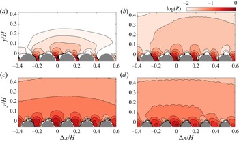
(a i–d i) Inter-layer correlation coefficient of  $v'$ fluctuations. Panels (a i–d i) represent cases C05–C08, respectively. The contours show the logarithm of the correlation coefficient, with levels from
 $-1.5$ to
 $-0.01$ with a step of 0.02. (a ii–d ii) Transfer entropy between different
 $y$ positions. Panels (a ii–d ii) represent cases C05–C08, respectively. The contours show the logarithm of the transfer entropy, with levels from
 $-6$ to
 $-2$ with a step of 1.

For lower porosity cases C05 and C06 (figure 4a i,b i), the correlation map shows a ‘neck’ around  $(y_1,y_2)=(0,0)$ that separates the contour into two parts, i.e. the part with both
 $y_1$ and
 $y_2$ above the interface, and the one involving porous medium flow (
 $y_1<0$ or
 $y_2<0$). Without loss of generality, we can consider
 $y_2$ (the vertical axis) as the position of the reference
 $v'$, and its correlated range is shown on the
 $y_1$ axis (the horizontal axis). The fluctuation
 $v'$ at the interface (
 $y_2=0$) has a quite strong connection with the flow below the interface (
 $y_1<0$), but a limited correlated range in the channel region (
 $y_1>0$). This is probably due to the scale separation between eddies in the near-wall region and the outer layer. As
 $y_2$ goes up to the channel (
 $y_2\ge 0$), the correlated range of
 $y_1$ increases linearly with
 $y_2$, which is associated with the growth of the scale of coherent structures. The correlated
 $y_1$ range increases more drastically when
 $y_2$ descends into the porous media area (
 $y_2<0$). In fact, the correlation coefficient between surface/subsurface flow can even exceed that of two points in the channel. This is direct evidence that the motions in the transitional layer of the porous medium are interacting with the flow structures in the boundary layer. As porosity grows (C07 and C08), the intensity of the correlation map increases, and the ‘neck’ between the channel region and the porous media region becomes ambiguous. However, the outline of the correlation map remains similar.
The correlation map provides insight into the connection of signals at different layers. However, as explained earlier, this method cannot discern between the two coupling directions. In the next section transfer entropy is used to clarify this problem.
3.2.2. Transfer entropy map
The same set of data as in § 3.2 is be used to compute transfer entropy, and the result is shown in figure 4(a ii–d ii). Since the input signals for transfer entropy are assigned as target or source, the  $y$ positions of the target and source
 $v'$ signals are defined as
 $y_{{target}}$ and
 $y_{{source}}$, respectively. For each set of
 $(y_{{target}},y_{{source}})$, the delay time
 $\Delta t$ is selected so that the maximum value of transfer entropy is reached, which is generally found in the range of
 $\Delta tU_b/H=[0,1]$. The optimal
 $\Delta t$ for signal pairs with an extremely weak causal link could be contaminated by noise. Nonetheless, this does not undermine the map of transfer entropy since we mainly focus on the areas with considerable information exchange.
In contrast to the correlation map, the transfer entropy map is asymmetrical, especially near and below the crest position. When the destination  $y_{{target}}$ is located in the channel region, the transfer entropy decays quickly as
 $y_{{source}}$ moves away from
 $y_{{target}}$. In contrast, for a target signal below the interface (
 $y_{{target}}<0$), the information flux from the channel flow maintains a high magnitude as
 $y_{{source}}$ rises, suggesting that the fluctuations below the interface are actively subject to the influence of channel flow. The magnitude of transfer entropy from the porous medium to the channel flow is almost negligible for the lowest porosity case C05. As the porosity increases, the information flux from below the interface to above (bottom-up effect) rises accordingly, but the top-down coupling always dominates for the cases tested.
The transfer entropy map illustrates clearly the asymmetry of the interaction between channel flow and porous medium, which cannot be identified by correlation due to its symmetry. Each coupling direction will be explored separately in the following sections.
3.3. Spatial structure of transfer entropy
In the previous section we explored the transfer entropy in the  $y$ direction, which elucidated the causal relation between the channel and porous medium flow. Note that only one streamwise location is selected, which is right in the middle of two nearby cylinders. In this section the influence of streamwise position on transfer entropy will also be investigated. However, instead of enumerating all possible combinations of spatial locations in § 3.2, we specify
 $v'$ in the midst of the top-layer cylinders, i.e. (
 $x_c/H=0,0.2,0.4,\ldots,10;y_c=-r_c$), as the representative signal of the porous medium, and explore the information flux between it and nearby spatial points.
As in previous sections, we first show the two-dimensional correlation map as a comparison with transfer entropy. With the reference location selected at  $(x_{{ref}},y_{{ref}})=(x_c,y_c)$, the definition of the correlation map differs from that in (3.10), i.e.
 \begin{equation} R_{vv}(\Delta x,y)=\max_{\Delta t}\left\{\frac{\overline{v'(t;x_{{ref}},y_{{ref}})v'(t+\Delta t;x_{{ref}}+\Delta x,y)}}{\sigma_{v'}(x_{{ref}},y_{{ref}})\sigma_{v'}(x_{{ref}}+\Delta x,y)}\right\}. \end{equation}
For each ( $\Delta x,y$) pair, the time shift
 $\Delta t$ is selected so that the correlation function inside the braces from the right-hand side of (3.11) reaches its maximum. The results are shown in figure 5. There is a strong correlation between the
 $v'$ of nearby upstream and downstream pore units for all cases tested. As discussed by Wang et al. (Reference Wang, Chu, Lozano-Durán, Helmig and Weigand2021a), this strong correlation can be attributed to the interaction of fluids in adjacent pores under the constraint of continuity. A strong up-welling motion at one pore could induce down-welling motions of nearby pore units. In addition, Kim et al. (Reference Kim, Blois, Best and Christensen2020) show the up-welling and down-welling motions at the permeable surface is under the modulation of large-scale structures from the channel flow. In particular, up-welling motions happen during the passage of a low-speed structure, while down-welling motions usually correspond to high-speed motions. This is also supported by the large-scale statistical structure in the channel region, which encapsulates the correlated pore unit below (figure 5).
Map of correlation coefficient  $R_{vv}(\Delta x,y)$ in
 $x$–
 $y$ plane. Panels (a–d) represent cases C05–C08, respectively. The reference point is located at the middle of cylinders, i.e.
 $(\Delta x,y)=(0,-r_c)$. The colour and the isolines show the logarithm of the correlation coefficient, with levels from
 $-2$ to
 $-0.02$ with a step of 0.02.

However, the question of coupling direction remains unanswered. Is it that the large-scale structure in the channel induces the up/down-welling motions at the permeable wall? Or are the up/down-welling motions contributing to the large-scale motions in the channel? This question will be answered in the next section.
3.3.1. Optimal information transfer locations
In this section the transfer entropy is computed with a similar set of signals as in the computation of the correlation map in § 3.3. As the first part, the information transfer from channel to porous medium ( $T_{c\rightarrow p}$) is inspected, with the vertical fluctuation
 $v'$ at the first-layer cylinder gap
 $(x_{c},-r_c)$ chosen as the target signal, and the
 $v'$ at (
 $x_{c}+\Delta x$,
 $y$) selected as the source signal. That is,
 \begin{equation} \tilde T_{c\rightarrow p}(y,\Delta x)=\max_{\Delta t}\{\tilde T_{v'_c\rightarrow v'_p}(\Delta t)\}, \end{equation}
where
 \begin{equation} \left. \begin{aligned} v'_c(t) & =v'(x_{c}+\Delta x,y,t),\\ v'_p(t) & =v'(x_{c},-r_c,t). \end{aligned} \right\} \end{equation}
The time delay  $\Delta t$ is chosen where
 $T_{c\rightarrow p}$ reaches a maximum for each set of source and target signals. Similarly, the transfer entropy map in the ‘bottom-up’ direction can be defined as
 \begin{equation} \tilde T_{p\rightarrow c}(y,\Delta x)=\max_{\Delta t}\{\tilde T_{v'_p\rightarrow v'_c}(\Delta t)\}, \end{equation}
where  $v'_c$ and
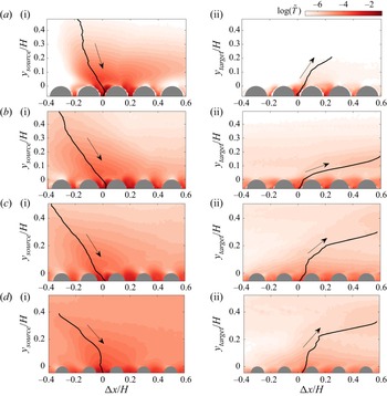
 $v'_p$ are the same as defined in (3.13). Figure 6(a i–d i) shows the map
 $T_{c\rightarrow p}$ for different cases that illustrate the variation of ‘top-down’ transfer entropy due to the spatial variation of the source signal. For all cases, the upstream locations have a larger influence on the porous medium. The solid lines in figure 6(a i–d i) illustrate the maximum transfer entropy locations at different
 $y$ layers. Hereafter, we refer to the points on the lines as the ‘optimal information transfer source’, since each of them has the maximum informative flux towards the porous medium. Note that the line of optimal source leans more towards the upstream direction with the increase of porosity. In addition to the optimal source, there are secondary sources at the nearby pore unit downstream for the low porosity cases C05 and C06 (figure 6a i–b i). It appears that the fluctuations at the downstream pore unit can also affect its neighbouring pore in the upstream. This is related to the inter-pore coupling effect shown by the correlation map in figure 5. Nonetheless, the strength and wall-normal range of the secondary source is generally limited compared with the optimal sources.
Spatial map of transfer entropy  $\tilde T$ in
 $x$–
 $y$ plane. The colours in panels (a i–d i) show the transfer entropy
 $\tilde T_{c\rightarrow p}$ in the direction from the channel to the porous medium (indicated by arrows) for cases C05 to C08, respectively. The vertical axis
 $y_{{source}}$ denotes the
 $y$ position of the source signal. Panels (a ii–d ii) represent the transfer entropy
 $\tilde T_{p\rightarrow c}$ in the bottom-up direction (indicated by arrows) for cases C05 to C08, respectively. Here
 $y_{{target}}$ is the wall-normal position of the target signal. The solid lines are the paths that connect the positions of maximum transfer entropy at each
 $y$ layer.

Figure 6(a ii–d ii) shows the map of ‘bottom-up’ transfer entropy  $T_{p\rightarrow c}$. For the same porosity, the magnitude of
 $T_{p\rightarrow c}$ is much smaller than
 $T_{c\rightarrow p}$ in the channel region. This is consistent with our observation in § 3.2. The main reason is the blockage of near-wall turbulence. The turbulence near the interface is highly energetic and chaotic, while the up- and down-welling motions in the porous medium are much weaker (see intensity profiles in figure 1b–d). The fluctuations near the interface are mainly driven by the self-sustaining cycle, and the information flux that comes from the porous medium is quite low. The strong turbulence in the buffer layer thus blocks the information of
 $v'_p$ from going further to the outer layer. Nevertheless, we can still draw lines of optimal target positions for bottom-up transfer. In the case of the lowest porosity (
 $\varphi =0.5$), we stop looking for maximum points above
 $y/H=0.2$ because the value of
 $\tilde T$ becomes extremely small and subject to statistical uncertainty. For all the cases, the optimal paths of ‘bottom-up’ transfer lean downstream. This is reasonable since the fluid ejected by the up-welling motion can be convected by the mean velocity of the channel.
Wang et al. (Reference Wang, Chu, Lozano-Durán, Helmig and Weigand2021a) inspected the full spectra of the channel flow and porous medium flow. They showed that the energy of the porous medium flow concentrates on the low-frequency modes, and has a large disparity with the central frequency of near-wall turbulence. For current observations, the turbulence in the channel flow is the driver while the fluid in the porous medium behaves as a passive damper. The porous medium flow accepts information from the channel flow and damps out the high-frequency modes, leaving only low-frequency fluctuations that are considerably weak. The details of this argument will be described in the next section.
3.4. Spectral-resolved transfer entropy
3.4.1. Surrogate method based on discrete wavelet transform
In this section the contribution of different frequency modes to the information flux at the interface region will be evaluated. Understanding the scale range of sending or receiving information is an essential step to unraveling the dynamics of time sequences. However, finding the connection between scale and causality is a non-trivial problem. Earlier attempts to obtain the desired frequency-resolved transfer entropy relied on narrow-band filtering of data from the information source and the information receiving target, followed by feeding the resulting narrow-band signals into a transfer entropy analysis (Besserve et al. Reference Besserve, Schölkopf, Logothetis and Panzeri2010; Wang et al. Reference Wang, Chu, Lozano-Durán, Helmig and Weigand2021a). However, this method could be sensitive to the choice of the band filter. A very narrow-band filter may cause false-positive results due to phase distortions. In addition, the information transfer between a source and a target within a specific narrow frequency band practically confines the analysis to the linear interaction regime, while information transfer can transform frequencies between source and target.
In the current work we adopt the surrogate data method from Pinzuti et al. (Reference Pinzuti, Wollstadt, Gutknecht, Tüscher and Wibral2020) to bypass the potential biases originating from narrow-band filtering. Instead of extracting a limited band from the original signals, this method substitutes the frequencies of interest with surrogate data representing the null hypothesis of no information transfer. The surrogates are produced by destroying the temporal order of the original signal at a specific scale range while keeping the remaining scales unchanged. The frequency specificity is obtained by evaluating the drop of transfer entropy with these surrogate data compared with the original one.
The flow chart for the computation of the frequency-specified transfer entropy, or spectral transfer entropy (STE), is illustrated in figure 7. The creation of surrogate data is the first and crucial step, which is achieved through the maximum overlap discrete wavelet transform (MODWT) method (Percival & Walden Reference Percival and Walden2000). The MODWT of a time series  $X = (X_0,\ldots, X_{N-1})$ of
 $J$ levels consist of
 $J$ vectors of wavelet coefficient
 $\tilde {\boldsymbol {W}}_1$,…,
 $\tilde {\boldsymbol {W}}_J$ and an additional vector
 $\tilde {\boldsymbol {V}}_J$, all with dimension
 $N$, which is computed as
 \begin{equation} \left. \begin{aligned} \tilde{\boldsymbol{W}}_j & =\tilde{\boldsymbol{\mathsf{W}}}_j X,\\ \tilde {\boldsymbol {V}}_J & =\tilde{\boldsymbol{\mathsf{V}}}_J X, \end{aligned} \right\} \end{equation}
where  $\tilde {\boldsymbol{\mathsf{W}}}_j$ and
 $\tilde {\boldsymbol{\mathsf{V}}}_J$ are
 $N\times N$ matrices, each row of which are the wavelet and scaling filter, respectively. The vector of wavelet coefficients
 $\tilde {\boldsymbol {W}}_j$ are associated with the underlying dynamics at a certain scale, and the coefficient
 $\tilde {\boldsymbol {V}}_J$ represents the unsolved low-frequency scale of
 $X$. If
 $J$ is set to
 $\lfloor { {\log }_2(N)} \rfloor$, any scale that is shorter than
 $N$ will be resolved by the wavelet coefficient
 $\tilde {\boldsymbol {W}}_j$. The nominal frequency band of the
 $j$th scale is
 $|f|\in (1/2^{j+1},1/2^j)$. If
 $\tilde {\boldsymbol {W}}_j$ and
 $\tilde {\boldsymbol {V}}_J$ are not modified, it is possible to reconstruct
 $X$ through the inverse MODWT,
 \begin{equation} X=\mathop{\varSigma}_{j=1}^{J}{\tilde{\boldsymbol{\mathsf{W}}}_j^{\rm T}\tilde{\boldsymbol{ W}}_j}+\tilde{\boldsymbol{\mathsf{V}}}_J^{\rm T}\tilde{\boldsymbol{V}}_J, \end{equation}
where the superscript  ${\rm T}$ denotes the transpose of the matrix. If we randomly shuffle the wavelet coefficient
 $\tilde {\boldsymbol { W}}_i$ at a specific level
 $i$, and replace the original
 $\tilde {\boldsymbol { W}}_i$ with the scrambled
 $\tilde {\boldsymbol { W}}'_i$ in (3.16), the reconstructed surrogate data
 $\check {X}$ will share the same energy distribution with the original signal
 $X$ (figure 7) in spectral space, yet the temporal order and phase relations in the frequency band represented by
 $\tilde {\boldsymbol {W}}_i$ are lost. For the same source signal, the STE with a frequency-specified target signal can be defined as the difference between the transfer entropy with original signals and that with the surrogate target signal, i.e.
 \begin{equation} \delta \tilde T_{Y\rightarrow \check{X}}(i)=\frac{ T_{Y\rightarrow X} - T_{Y\rightarrow \check{X}_i}}{H(X_t|X_{t-1})}, \end{equation}
where  $\check {X}^i$ is the putative data for
 $X$ with the temporal shuffled
 $i$th mode as illustrated in figure 7. The intrinsic uncertainty of
 $X$ is used for normalization. Similarly, the STE with frequency-specified source signal is defined as
 \begin{equation} \delta \tilde T_{\check{Y}\rightarrow X}(i)= \frac{ T_{Y\rightarrow X} - T_{\check{Y}_i\rightarrow X}}{H(X_t|X_{t-1})}, \end{equation}
where  $\check {Y}_{i}$ is the surrogate data for
 $Y$ with the temporal shuffled
 $i$th mode. It should be noted that the surrogate tests for
 $X$ or
 $Y$ need to be implemented multiple times to achieve statistical convergence, as transfer entropy can fluctuate with the random permutation state in
 $\check X$ or
 $\check Y$. In the current study, we take the median of the 100 runs as the final result.
The calculation of spectral transfer entropy using surrogate data. The variables involved with the surrogate data are highlighted with shaded blocks.

To illustrate the computation procedure described above, we use again the fluctuations  $v'_1(t)$ at
 $y=-r_c$ and
 $v'_2(t)$ at
 $y=0$ as in § 3.2. The STE with frequency-specified source, i.e.
 $\delta \tilde T_{\check {v}'_2\rightarrow v'_1}$, will be computed. As the first step, the time sequences of
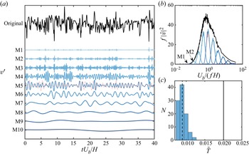
 $v'_2$ are decomposed into a series of MODWT modes, as shown in figure 8(a). The maximum mode order that can be achieved is
 $\lfloor { {\log }_2(2000)} \rfloor =10$. The modes’ scales grow exponentially with their order, with the fourth and fifth modes appearing to be the most active of them. This is verified by the power spectra in figure 8(b). The original spectrum can be recovered by combining all the spectra of the MODWT modes. Note that the first mode is extremely weak and can be barely identified in the spectra.
Generating surrogate data using maximum overlap discrete wavelet transform (MODWT). (a) The decomposition of time series of  $v'$ fluctuation (black solid line) with MODWT. The first to tenth modes are denoted by blue solid lines, and the scrambled fifth mode is shown by the red dashed line. (b) The power spectra of the original time series (black solid line) and MODWT modes (blue solid lines). The spectrum of the scrambled fifth mode is shown by the red dashed line. The spectra of the first and second modes are indicated by arrows M1 and M2, respectively. (c) The distribution of transfer entropy using surrogates data. The dashed vertical line indicates the median value. Transfer entropy of the original time series is indicated by the vertical solid line.

As described above, the surrogate data are created by scrambling the temporal order of the wavelet coefficient at a certain level. In the current study, we adopted the block permutation method (Breakspear, Brammer & Robinson Reference Breakspear, Brammer and Robinson2003). This method divides the wavelet coefficients into smaller blocks, and then randomly permutes the temporal order of them. For this study, the block size is chosen to be  $\Delta T_{block}U_b/H=4$ such that the original energy and scale are substantially conserved. Other block sizes might be used as long as they allow for considerable phase order destruction while maintaining the scale feature. Figure 8(a) shows an example of a scrambled fifth mode with the red dashed line, and its corresponding spectrum is illustrated in figure 8(b) with the red dashed line. It shows that both the energy and scale of the surrogate fifth mode are almost unchanged, but the original temporal order of the phase is completely destroyed. Therefore, the information transfer related to the frequency component in the fifth mode is eliminated. Combining the scrambled fifth mode and the remaining unchanged modes, the surrogate data
 $\check {v}'_{2}$ is generated with (3.16).
Taking  $v'_1$ as the target signal, the STE can then be calculated by measuring the difference between
 $T_{v'_2\rightarrow v'_1}$ and
 $T_{\check {v}'_{2}\rightarrow v'_1}$. The computation procedure of
 $T_{\check {v}'_{2}\rightarrow v'_1}$ is performed 100 times to assess the statistical significance of the outcome, and the distribution of
 $T_{\check {v}'_{2}\rightarrow v'_1}$ is shown in figure 8(c) as a histogram. The dashed line indicates the median of the distribution of
 $T_{\check {v}'_{2}\rightarrow v'_1}$, and the solid line indicates the value of
 $T_{v'_2\rightarrow v'_1}$. In this case, all the samples of surrogate-based transfer entropy are significantly lower than the original transfer entropy, while the median of
 $T_{\check {v}'_{2}\rightarrow v'_1}$ is more than 50 % lower than the original value, showing that the fifth mode is responsible for a considerable amount of information flux.
3.4.2. Transfer entropy spectra
In this section the computation of STE established in § 3.4.1 is extended from the permeable interface to the channel centre. As discussed in § 3.2.2, the porous medium flow can scarcely impact the outer region of the boundary layer, and the transitional layer is subject to strong influence from the surface flow. Moreover, the turbulent boundary layer consists of a wide spectrum of scales, such as near-wall eddies, outer scale motions in the log layer, as well as KH-type eddies (Breugem et al. Reference Breugem, Boersma and Uittenbogaard2006; Wang et al. Reference Wang, Chu, Lozano-Durán, Helmig and Weigand2021a). In contrast, the porous medium flow features mainly low-frequency fluctuation (Chu et al. Reference Chu, Wang, Yang, Terzis, Helmig and Weigand2021). This is demonstrated by the power spectra of  $\varPhi _{vv}$ in figure 9 (isolines). In contrast to the spectra of the channel flow, which is widely distributed across the whole spectral domain, the turbulent kinematic energy below
 $y=0$ concentrates primarily in the range of
 $U_b/(fH)\ge 3$. Therefore, we will simply look at the frequency specificity in the surface flow and leave the subsurface flow untouched.
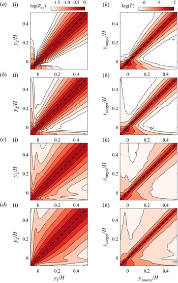
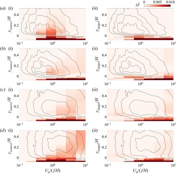
The map of spectral transfer entropy. The colour contours in the left-hand side panels (a i–d i) show the spectral transfer entropy with a frequency-specified source signal, and with a frequency-specified target signal in right-hand side panels (a ii–d ii). Rows (a–d) represent cases C05–C08, respectively. The power spectra  $\varPhi _{vv}$, which are normalized by their respective maximum, are superimposed as isolines, whose levels are from 0.2 to 0.8 with a step of 0.2.

Similarly as in § 3.2.2, the vertical fluctuation at the gap between the top-layer cylinders ( $y=-r_c$) is defined as
 $v'_c$ to represent the mass flux originating from the porous medium. The fluctuation in the channel is named as
 $v'_c$ and will be decomposed by MODWT for the surrogate data generation procedure. The colour contours in figure 9(a i–d i) show the map of STE in the ‘top-down’ direction, namely
 $\delta \tilde T_{\check v_c'\rightarrow v_p'}$ . For the lower porosity case C05, the strongest
 $\delta \tilde T$ concentrate in the near-interface region. The most active information transfer scale range above the interface is found in
 $U_b/(fH)\in [0.6,1.2]$ (
 $U_bu_\tau /(f\nu )\in [300, 600]$), which is consistent with the energetic scale of the spectrum
 $\varPhi _{vv}$ at the same layer. This is close to the scale of quasi-streamwise vortices in smooth wall-bounded flow as the permeability of case C05 is quite low (
 $\sqrt {K_{xx}}^{p+}\approx 5$). For example, the numerical simulation of Jeong et al. (Reference Jeong, Hussain, Schoppa and Kim1997) reported that the average streamwise extent of quasi-streamwise vortices is approximately 250 wall units. The experiment of Jodai & Elsinga (Reference Jodai and Elsinga2016) detected quasi-vortices with tomographic particle image velocimetry, which have a streamwise extent of 150–250 wall units. Jiménez (Reference Jiménez2012) computed the streamwise spectra of enstrophy, the peak is located around 300 wall units. Note that here we interpret frequency
 $f$ into streamwise extent with a fixed convection speed
 $U_b$ under Taylor's hypothesis, which may cause an overestimation of the spatial scale of near-wall structures. In the next section we will directly measure the spatial extent of informative flow motions from the statistical structure.
As the porosity increases, the scale range of the information sources shifts to the low-frequency side. For the highest porosity case C08, there is a significant contribution from the scale range of  $U_b/(fH)\approx 2.4$–
 $9.6$, which is consistent with the scale of KH-type eddies. For example, Finnigan, Shaw & Patton (Reference Finnigan, Shaw and Patton2009), Kuwata & Suga (Reference Kuwata and Suga2017) and Suga et al. (Reference Suga, Okazaki, Ho and Kuwata2018) reported that the wavelength of KH eddies is in the range of
 $\lambda _x/\delta _p= 3.4$–
 $5.5$ (
 $\delta _p$ is the boundary thickness). White & Nepf (Reference White and Nepf2007) reported that the most unstable mode has a frequency of
 $(f\theta )/\bar {U}\approx 0.032$ (
 $\theta$ and
 $\bar {U}$ being the momentum thickness and mean velocity of the whole test section), which is equivalent to
 $U_b/(fH)\approx 4$ when normalized with channel width and bulk velocity of the channel. The rise of the informative scale in the near-wall region appears to be linked with the growth of the energetic scale in the power spectrum as the porosity increases. Moreover, the informative scale rises when the source signal moves to a higher position, regardless of the energetic scale there. This shows that when the source and target signals are separated by a large distance, the high-frequency information flux in between is dissipated but the low-frequency information is preserved.
The panels on the right-hand side of figure 9(a ii–d ii) show STE in the ‘bottom-up’ direction with frequency specified  $v'_c$, i.e.
 $\tilde T_{v'_p\rightarrow \check {v}'_c}$. Remember that
 $\tilde T_{v'_p\rightarrow \check {v}'_c}$ shows the amount of information received by the channel flow
 $v'_c$ from the porous medium flow
 $v'_p$ at each frequency range. In accordance with the spatial map of transfer entropy in § 3.2.2, the influential
 $y$ range of the porous medium flow is restricted to the near-wall region. For case C05, the most receptive scale in the channel is
 $U_b/(fH)\in [0.6, 1.2]$, same as the informative scale in
 $\tilde T_{v'_p\rightarrow \check {v}'_c}$ (figure 9a i), demonstrating that the surface/subsurface interaction in both directions is aided by near-wall vortices. As porosity increases, the scale range
 $U_b/(fH)\in [2.4,9.6]$ associated with KH-type eddies becomes more responsive with a certain amount of information flux up to the middle of the channel.
3.5. Statistical structure of informative events
In earlier sections the statistics of transfer entropy were examined in spatial and spectral space. Here, we connect transfer entropy with specific flow motions. We will try to depict the informative flow process by correlating local transfer entropy with flow motions. Following the idea of local transfer entropy, the STE can also be reformulated as the expectation value of a local variable. Without normalization, the STE with a frequency-specified source can be reformulated as
 \begin{align} \delta T_{\check{Y}\rightarrow X}&=T_{Y\rightarrow X}-T_{\check{Y}\rightarrow X}\nonumber\\ &=E\left[\zeta_{Y\rightarrow X}-\zeta_{\check{Y}\rightarrow X} \right] \nonumber\\ &=E\left[\delta\zeta_{\check{Y}\rightarrow X} \right], \end{align}
where  $\zeta _{Y\rightarrow X}$ is the same as defined in (3.5) and
 $\zeta _{\check {Y}\rightarrow X}$ is the local transfer entropy calculated with surrogate signal sets, which is defined as
 \begin{equation} \zeta_{\check{Y} \rightarrow X}(t;\Delta t)=\log _{2} \frac{p\left(x_{t} \mid x_{t-1}, \check{y}_{t-\Delta t}\right)}{p\left(x_{t} \mid x_{t-1}\right)}. \end{equation}
Substituting (3.5) and (3.20) into (3.19), the scale-resolved local transfer entropy  $\delta \zeta _{\check {Y}\rightarrow X}$ can then be derived as
 \begin{equation} \delta\zeta_{\check{Y} \rightarrow X}(t;\Delta t)=\log _{2} \frac{p\left(x_{t} \mid x_{t-1}, y_{t-\Delta t}\right)}{p\left(x_{t} \mid x_{t-1}, \check{y}_{t-\Delta t}\right)}. \end{equation}
Similarly, the transfer entropy with a frequency-specified target can be written as  $\delta T_{Y\rightarrow \check {X}}=E[\delta \zeta _{Y\rightarrow \check {X}}]$, which is defined as
 \begin{equation} \delta\zeta_{Y \rightarrow \check{X}}(t;\Delta t)=\log _{2} \frac{p\left(x_{t} \mid x_{t-1}, y_{t-\Delta t}\right)p\left(\check{x}_{t} \mid \check{x}_{t-1}\right)}{p\left(\check{x}_{t} \mid \check{x}_{t-1}, y_{t-\Delta t}\right)p\left(x_{t} \mid x_{t-1}\right)}. \end{equation}
Note that we derive the local STE  $\delta \zeta$ from the non-normalized STE as we are only concerned with the relative contribution of local events to the total amount of information flux, i.e.
 $\delta \zeta /\delta T$. Therefore, there is no need to involve the denominator in (3.17) and (3.18). The local STE
 $\delta \zeta$ can be interpreted as the contribution of instantaneous events to the total loss in transfer entropy owing to the absence of information at a specific time scale. With the local frequency-specified transfer entropy
 $\delta \zeta$ defined, it is now possible to relate flow motions to the causal interaction at scales of interest. To do so, we use LSE, in which the variable to be estimated is assumed to be a linear function of the event variable. In this case, we wish to discover the most probable flow structure under an informative event. The predicted flow field
 $\tilde v$ may be obtained by multiplying the coefficient matrix
 $C$ with the amplitude of local spectra transfer entropy
 $\delta \zeta$, i.e.
 \begin{gather} C(\Delta \tau;x,y)=\frac{\overline{v'(t-\Delta \tau;x,y)\delta \zeta(t;\Delta t)}}{\sigma_{\delta \zeta}^2}, \end{gather}
 \begin{gather} \tilde v(t-\Delta \tau;x,y)= C(\Delta \tau;x,y)\delta\zeta(t), \end{gather}
where  $\Delta \tau$ is the shifted time interval between the snapshot of
 $v'$ and
 $\delta \zeta$, and
 $\Delta t$ is the time delay between the source and target signal for the computation of
 $\delta \zeta$. When
 $\Delta \tau =0$, the field of
 $v'$ corresponds to the state of the target signal involved in
 $\delta \zeta$; when
 $\Delta \tau =\Delta t$, the snapshot of
 $v'$ illustrates the state of the source signal. In this study, the time interval
 $\Delta \tau$ will be changed from 0 to
 $\Delta t$ to study the evolution of flow structures during the information transfer process. The LSE of the streamwise component
 $\tilde u$ can be acquired in a similar approach by replacing
 $v'$ with
 $u'$ in (3.23).
Note that  $\delta \zeta$ depends on multiple variables, such as the choice of time delay
 $\Delta t$, spatial position of source and target signals (
 $Y$ and
 $X$), specified scale range, etc. It would be impossible to list them all in this paper, so only the most representative results are shown here. We will fix the time delay
 $\Delta t$ to the value that corresponds to the maximum
 $\delta T$ as in the last section. Recall that in § 3.4.2, mainly two types of flow structures are confirmed to be involved in the causal interaction. The most active information transfer scale for the low porosity case (
 $\varphi =0.5$) falls in the range
 $U_b/(fH)\in [0.6,1.2]$, which is assumed to be linked to near-wall vortices. In contrast, the frequency range (
 $U_b/(fH)\in [2.4,4.8]$) of KH-type eddies gradually dominates the coupling process in higher porosity cases (
 $\varphi =0.7,0.8$). In the following, both of the two scenarios above will be illustrated by LSE structures.
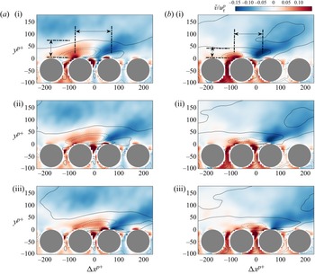
Figure 10 shows the first scenario where the velocity fields are associated with local STE  $\delta \zeta /\sigma _{\delta \zeta }=1$ at the frequency range
 $U_b/(fH)\in [0.6,1.2]$ for case C05. The upper row (figure 10a i–a iii) shows the ‘top-down’ coupling process with the target and source signals picked from
 $y=-r_c$ and
 $y=0$, respectively. The results of the opposite coupling direction are obtained by switching the source and target, which is shown in the bottom row (figure 10b i–b iii). From left to right, statistical flow motions shown in the three columns correspond to a time shift
 $\Delta \tau$ of
 $\Delta t$ ,
 $\Delta t/2$ and
 $0$, respectively. To put it more clearly, the leftmost column shows the initial state of the causal event, the rightmost column depicts the final state and the centre column depicts the intermediate state. For both coupling directions, the whole causal process shows essentially the passage of a Q2 motion (
 $\tilde u<0,\tilde v>0$) over the interface, with up- and down-welling motions at the gap between cylinders (
 $\Delta x=0$). However, there is a few subtle differences. The vertical flux at the cylinder gap (
 $\Delta x=0$) for the ’top-down’ coupling is originally oriented towards the porous medium, but due to the influence of the Q2 structure coming from upstream, it turns positive. The flux at
 $\Delta x=0$ for the ’bottom-up’ coupling is towards the channel, which transports low-speed fluids from the porous medium up to the interface, enhancing the Q2 events above. Despite the fact that scale selection is only done in the computation of
 $\delta \zeta$, the statistical structure's streamwise scale correctly restores the scale we chose. To quantify the spatial extents of these information events, the distance between the positive and negative peaks of
 $\tilde v$ is measured at
 $y^{p+}=17$, which corresponds to the wall-normal position of maximum
 $\sigma _{v'}$ (figure 1b). The
 $y$ extent of the ejection motions is also identified. An illustrative sketch of the spatial extent is shown in figure 10(a i,b i). For the top-down coupling, the distance between the two peaks is
 $L_x^{p+}=130$, which corresponds to a wavelength of
 $\lambda _x^{p+}=2L_x^{p+}=260$, and the wall-normal extent is
 $L_y^{p+}=55$. As a comparison, Kuwata & Suga (Reference Kuwata and Suga2017) investigated permeable wall-bounded flow at
 $Re_\tau ^{p+}=177\unicode{x2013} 399$ with permeability
 $\sqrt {K}^{p+}=5.5$–
 $11.6$. They reported that the streamwise wavelength of
 $v'$ is
 $\lambda ^{p+}_x=200$–
 $300$ at
 $y^{p+}=13$. As discussed in the last section, this scale is consistent with the quasi-streamwise vortices (Jeong & Hussain Reference Jeong and Hussain1995; Jodai & Elsinga Reference Jodai and Elsinga2016). The structures for bottom-up coupling are smaller with
 $L_x^{p+}=79$ (
 $\lambda _x^{p+}=158$) and
 $L_y^{p+}=37$. The shortened range is expected since the ‘bottom-up’ event under the influence extent of one single pore unit is limited in both streamwise and wall-normal dimensions.
The LSE of velocity field over local casual events for a low porosity porous medium (C05,  $U_b/(fH)\in [0.6,1.2]$). The coloured contour shows the
 $\tilde v$, and the isolines indicate
 $\tilde u$ with positive and negative levels denoted by solid and dashed lines, respectively. The levels are from
 $-0.1$ to 0.1 with a step of 0.05. Panels (a i–a iii) denote the ‘top-down’ process, and panels (b i–b iii) denote the ‘bottom-up’ process. Rows 1–3 correspond to the flow motions that are
 $\Delta t$,
 $\Delta t/2$ and
 $0$ ahead of the local informative event,
 $\Delta t$ being the time delay of the transfer entropy. The configuration above also applies for figure 11.

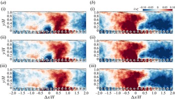
The LSE of velocity field over local casual events for a high porosity porous medium (C08,  $U_b/(fH)\in [2.4,4.8]$). For the plotting configuration, see figure 10.

Figure 11 shows the second scenario, in which the informative flow motions for the high porosity case C08 are approximated with local STE  $\delta \zeta /\sigma _{\delta \zeta }=1$ in the frequency range
 $U_b/(fH)\in [2.4,4.8]$. The configuration of figure 11 is the same as in figure 10. The flow fields for ‘top-down’ coupling (figure 11a i–a iii) depict the passage of a large Q4 structure (
 $\tilde u>0, \tilde v<0$) over the detecting point
 $\Delta x=0$. This leads to a variation of flux at the cylinder gaps. The spatial extent of the structures in the ‘top-down’ events is a bit challenging to determine as it varies in the
 $y$ direction. Close to the permeable wall (
 $y/H<0.4$), the streamwise wavelength of the local sweep/ejection motions is about
 $\lambda _x/H\approx 1$. As
 $y$ further elevates, the wavelength increases to
 $\lambda _x/H\approx 2$–
 $4$. The increase of informative scale in the
 $y$ direction is consistent with the result of STE in figure 9(d i). On the other hand, the ’bottom-up’ coupling process (figure 11b i–b iii) depicts fluid being ejected from underneath the interface and mixed with the large-scale Q2 motion (
 $\tilde u<0, \tilde v>0$) in the channel. The
 $\tilde u$ and
 $\tilde v$ structures have a streamwise wavelength of
 $\lambda _x/H\approx 2$–
 $4$ and occupy the whole channel region. As discussed in § 3.4.2, this scale is consistent with those of KH eddies reported by previous researchers (White & Nepf Reference White and Nepf2007; Suga et al. Reference Suga, Okazaki and Kuwata2020). However, it is noted that the up-welling motion at the interface only slightly changes the shape of the front line of the Q2 structure above the cylinders. This is in line with the prior observations in § 3.2.2 that the ’bottom-up’ coupling mainly affects the near-interface region.
3.6. Application of causal inference in remote sensing
The variation of spatial and spectral statistics related to transfer entropy illustrates the underlying causal properties of the coupling process at the interface. The turbulent motions in the channel, including near-wall vortices and KH-type eddies, have a significant causal influence on the up- and down-welling motions between cylinders, suggesting that it is possible to estimate the mass flux across the interface with information from the channel region. In fact, predicting variables at the wall using remote probes is a widely applied strategy in the modelling of wall-bounded flows (Hosseini, Martinuzzi & Noack Reference Hosseini, Martinuzzi and Noack2016; Encinar & Jiménez Reference Encinar and Jiménez2019; Kim & Lee Reference Kim and Lee2020; Guastoni et al. Reference Guastoni, Guemes, Ianiro, Discetti, Schlatter, Azizpour and Vinuesa2021). In previous works, the configuration of the input of the models, such as the placement and temporal resolution of the probes, is largely empirical and relies on posterior results. In this section we will demonstrate that transfer entropy can be used as a metric to evaluate the quality of input signals for a neural network model. On the other hand, the performance of a neural network provides a solid validation of the statistical results of transfer entropy in earlier sections.
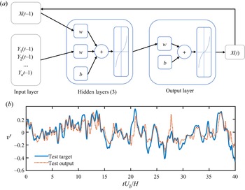
The architecture of a neural network used in the current study is shown in figure 12(a), which is a nonlinear autoregressive exogenous neural network (McCulloch & Pitts Reference McCulloch and Pitts1943; Lozano-Durán et al. Reference Lozano-Durán, Bae and Encinar2020). The target signal  $X(t)$ to be predicted is set as the fluctuation
 $v'(t)$ in the midst of the top-layer cylinders (
 $y=-r_c$). The input signals consist of both the feedback of
 $X$, which is the past state of
 $X$ at time
 $t-1$, and the exogenous input
 $Y(t-1)$, which is the history state of
 $v'(t)$ with wall-normal position
 $y>-r_c$. Here we only use one time step from the history of
 $X$ and external input
 $Y$ so that it is consistent with the embedding dimension of transfer entropy defined in (3.1). Note that this set-up is only adopted merely for the purpose of allowing it to be directly compared with the definition of transfer entropy. One might choose to include more history steps of
 $X$ and
 $Y$ to improve prediction performance. The number of exogenous input
 $n$ may also vary depending on the requirement. In the current study, both single and multiple exogenous inputs will be tested. The activation function for the hidden layers is the hyperbolic tangent sigmoid transfer function. The neural network is trained using Levenberg–Marquardt backpropagation with three hidden layers. The time sequences are randomly divided into three groups, training (80 %), validation (10 %) and test sets (10 %). The training is terminated when the damping factor of the Levenberg–Marquardt algorithm exceeds
 $10^{10}$ or the gradient of performance falls below
 $10^{-7}$.
(a) The architecture of the nonlinear auto-regressive exogenous neural network used in the current study; (b) comparison between the target signal (C05,  $v'$ fluctuation at
 $y=-r_c$) and the output of one of the trained neural network.

As an example, figure 12(b) compares a target time series from the test group with the one predicted by the neural network. External input here is  $v'$ at the crest height
 $y=0$. Due to the limited information input, the output of the neural network recovers the target sequence's major peaks but also has numerous deviations from the original signal. We measure the performance of the neural network quantitatively by mean squared error (MSE)
 $\epsilon$, which is defined as
 \begin{equation} \epsilon=\frac{\langle(X-X')^2\rangle}{\sigma^2_{X}}, \end{equation}
where  $X'$ is the predicted time series and
 $\sigma _{X}$ is the standard deviation of the target signal
 $X$. We extend our test by replacing the exogenous input as
 $v'$ at different wall-normal positions. Figure 13(a) shows the variation of
 $\epsilon$ as a function of the wall-normal distance
 $\Delta y$ between the exogenous input and the target signal. The prediction error approaches zero when the input signal is chosen to be very close to the cylinder gap, and increases as the elevation of the wall-normal position of the input signal. This is consistent with the spatial map of transfer entropy in figure 6(a i–a iv), where the magnitude of transfer entropy from channel to the porous medium decreases monotonously with increasing
 $y$.
The mean squared prediction error of the neural network as functions of the (a) source-target distance  $\Delta y$, and (b) spectral component of exogenous input signal.

The spectral component of the input may also affect the neural network's performance, which can be assessed using a similar surrogate technique as in § 3.4.2. Instead of using only one series of  $v'$, we expand the number
 $n$ of the exogenous input to 10, which are
 $v'$ sequences extracted from 10 wall-normal positions that are evenly distributed in the range
 $0< y/H<0.5$. Note that we avoid taking the points that are not ‘remote’ enough from the target as inputs in this remote sensing model. Furthermore, in § 3.4.2 the spectrum transfer entropy indicates weak dependence on the
 $y$ location, so we employ fluctuations at multiple
 $y$ levels as input to achieve a moderate predicting performance. The surrogate input
 $\check Y$ is constructed by disrupting the temporal order of a certain MODWT mode of these input signals while keeping the other modes intact, as described in § 3.4.2. After the training is complete, the MSE for altered input
 $\epsilon _{\check Y}$ is compared with the error level using the original
 $Y$ signals, i.e.
 $\epsilon _{Y}$, and the rise of the MSE owing to the destructed modes
 $\delta \epsilon =\epsilon _{\check Y}-\epsilon _{Y}$ represents the target signal's dependence on specific scale ranges. The result of
 $\delta \epsilon$ is shown in figure 13(b). For
 $\varphi =0.5$, the MSE has a peak at
 $U_b/(f_cH)\approx 1.2$, which falls exactly in the informative frequency range indicated by ‘top-down’ STE in figure 9(a i). For higher porosity cases
 $\varphi \ge 0.6$, the peaks move toward the larger-scale side
 $U_b/(f_cH)\ge 2.4$, suggesting the influence of outer-scale eddies (e.g. KH-type eddies) starting to dominate. This is also consistent with the trend illustrated by the STE in figure 9(a ii–a iv).
The performance of a neural network-based remote sensing model is a straightforward indicator of how causal the input signal is to the target signal. Despite the fact that the model is simply data driven and lacks physical interpretation, the information included in the external input is exploited by the neural network to generate the output. As a result, the prediction error reflects, to a certain extent, the missing information from the exogenous input about the target, which is the counterpart of the information flux represented by the definition of transfer entropy. In this sense, the prediction performance of the neural network provides a validation of the theoretical conclusions of transfer entropy. Inferring causal relationships merely based on the performance of a data-driven model, on the other hand, is not as robust and efficient as explicitly analysing the transfer entropy, because the results may depend on the choice of model types and the training procedure can be time consuming. Therefore, statistical results of transfer entropy might be employed as an auxiliary metric for screening ideal qualities of input signals, such as spatial location or temporal step, etc. In this way, one could more directly narrow down to the optimized inputs with maximum information flux to the target signal, thus accelerating the trial and error process and avoiding unnecessary computation costs.
4. Concluding remarks
In the current study the causal relationship between surface and subsurface flow is investigated with interface-resolved DNS data. Using turbulent fluctuations as the source and target signal, we calculate the transfer entropy between the top-layer pores and a wide range of positions in the channel. The maps of the spatial distribution of transfer entropy illustrate that the information flux from the porous medium to the free flow is limited to the near-wall region, even for the highest porosity case. On the other hand, the causal interaction in the ‘top-down’ direction is significantly stronger, and there is still observable causality between a higher layer of the channel flow (up to  $y/H=0.2$) and flow motions at top-layer pores. Based on the spatial map of transfer entropy, a path is illustrated connecting the optimal information transfer positions at each
 $y$ layer. The path from channel to porous medium connects the gap between cylinders with upstream locations in the channel, while the ‘bottom-up’ path is leaning towards the downstream. This is an intuitive conclusion that the up- and down-welling motions at the interface are influenced by the upstream flow motions in the channel, and affect downstream locations. However, the spatial transfer entropy map and the optimal path proved this conclusion in a quantitative way, which could help establish predictive models for the surface/subsurface flow system.
The dependency of transfer entropy on frequency range is also explored with a surrogate strategy. We measure the drop of information flux using surrogate signals, which are generated by replacing the original fluctuations at a certain frequency range with non-informative noise. This strategy is more robust than the band-filtering method against phase distortion error. The turbulent kinetic energy of the subsurface flow mainly resides in very-low-frequency modes, so we only inspected the dependency of transfer entropy on the scales of channel flow. For the low porosity case (C05), the frequency range of the strongest contribution to transfer entropy appears at  $U_b/(fH)\in [0.6,1.2]$, which conforms with the peak of the power spectrum
 $\varPhi _{vv}$ at the near-wall region, and is associated with the near-wall vortices. As porosity increases, the role of larger-scale structures begins to dominate. The scale range of
 $U_b/(fH)\in [2.4,9.6]$ is significant for the highest porosity case (
 $\varphi =0.8$), indicating the important role of KH-type eddies.
To further identify the flow motions associated with causal interaction, the concept of local transfer entropy is introduced, which measures the contribution of transient events. The cumulative spectra of local transfer entropy show that the predictive events tend to be those with a strong source signal  $Y$, and a relatively weak target
 $X$ (figure 3). Furthermore, we computed the LSE of the velocity field with respect to the local predictive events. For the ‘top-down’ coupling, the statistical flow motion shows the passage of sweeping or ejection motions over the reference pore unit. For the ‘bottom-up’ direction, the flow structure indicates mass flux across the interface due to up/down-welling motions. The scale of the structures has a direct correspondence with the selected frequency range of the STE.
The statistics of transfer entropy reveal that the channel flow plays a driving force in surface/subsurface interaction. This lays a theoretical foundation for remote sensing the up/down-welling motions at the interface with the information from the channel. On the other hand, constructing such predictive models may help consolidate the conclusions from transfer entropy. In the current study we use a nonlinear exogenous neural network to build test models, in which the prediction of the target signal relies on the information from the external input. The test result shows that the prediction accuracy of the same model decreases monotonously with the  $y$ positions of the input signal, which is consistent with the spatial map of transfer entropy in § 3.2.2. In addition, the scale dependence of input signals is evaluated by masking a certain frequency range of the input signal. The deterioration of the prediction performance in the absence of a certain mode reveals the amount of information carried by the corresponding frequency range, and the result conforms to that of STE.
To summarize, we inspected the interaction between the channel and porous medium flow using information-theoretic tools. The dependence of causal relations on the spatial location and spectral component of the turbulent fluctuations is measured quantitatively and validated by a test based on a neural network. In the current study we investigated the causality among the most basic flow variables, i.e. turbulent fluctuations. Previous studies (Kim & Lee Reference Kim and Lee2020; Guastoni et al. Reference Guastoni, Guemes, Ianiro, Discetti, Schlatter, Azizpour and Vinuesa2021) also considered pressure and wall-shear stress as important variables in modelling the permeable interface. In addition, advanced network architecture, such as physics-informed neural networks (Raissi, Perdikaris & Karniadakis Reference Raissi, Perdikaris and Karniadakis2019), provide an architecture that allows the physics of a flow to be integrated into the network. Therefore, future research may focus on causal analyses of higher-order flow variables and the development of causality-informed neural networks.
Acknowledgements
We acknowledge the support by the Stuttgart Center for Simulation Science (SimTech). All authors gratefully acknowledge the access to the high performance computing facility Hawk at HLRS, Stuttgart.
Funding
The study is funded by Deutsche Forschungsgemeinschaft (DFG, German Research Foundation) project SFB1313 (project no. 327154368) and under Germany's Excellence Strategy-EXC2075-390740016. A.L.-D. was supported by the National Science Foundation under grant no. 032707-00001.
Data availability statement
The data that support the findings of this study are available from the corresponding author upon reasonable request.
Declaration of interests
The authors report no conflict of interest.