
1 Introduction
Surfactants have extraordinarily widespread uses as cleaning, dispersing, emulsifying, foaming and anti-foaming agents, and their adsorption at fluid interfaces has been studied extensively (Miller Reference Miller1988; Schramm, Stasiuk & Marangoni Reference Schramm, Stasiuk and Marangoni2003; Bouchemal et al. Reference Bouchemal, Briancon, Perrier and Fessi2004). Ionic surfactants are particularly effective at stabilizing dispersions, since the charge provides an electrosteric barrier to coalescence, which would otherwise promote macroscopic phase separation by minimizing interfacial energy. On the other hand, the charge also provides an electrostatic penalty for surfactant adsorption, increasing the interfacial energy. Thus, mixtures of charged and uncharged surfactants can be especially effective for optimizing the tradeoff between minimizing the surface energy and maximizing electrosteric repulsion. Such considerations are fundamental to well-established and contemporary technologies harnessing nano- and micro-emulsions (Gupta et al. Reference Gupta, Eral, Hatton and Doyle2016; Hashemnejad et al. Reference Hashemnejad, Badruddoza, Zarket, Ricardo Castaneda and Doyle2019).
The significant role of charge in influencing adsorption is demonstrated by the role of added salt in the surface tension of interfaces bearing ionic surfactants. Borwankar & Wasan (Reference Borwankar and Wasan1988) developed a theory for the surface tension that captures this effect. Their isotherm, which incorporates a Gouy–Chapman model of the electrostatic and translational entropy of the diffuse double layer, provided an excellent fit to surface-tension measurements. However, the model was drawn into question due to the very high electrostatic surface potentials that it predicts, thus motivating models that invoke counterion binding (Kralchevsky et al. Reference Kralchevsky, Danov, Broze and Mehreteab1999). These reduce surface potentials to values that are considered compatible with  $\unicode[STIX]{x1D701}$-potentials inferred by electrophoretic mobility measurements on surfactant-stabilized emulsion drops, but the correspondence may be questioned due to the challenge of interpreting electrophoretic mobility.
For example, mobilities are routinely measured using commercial electrophoretic light-scattering instruments and converted to surface potentials using the well-known Smoluchowski formula (Russel, Saville & Showalter Reference Russel, Saville and Showalter1989), which predicts a linear relationship between the mobility and  $\unicode[STIX]{x1D701}$-potential for particles that are much larger than the Debye length
 $\unicode[STIX]{x1D705}^{-1}$. However, for highly charged interfaces, it is perhaps less well known that mobility can be significantly lower than predicted by the Smoluchowski formula, e.g. as captured by the standard electrokinetic model (O’Brien & White Reference O’Brien and White1978). Overlooking this correction would underestimate the actual
 $\unicode[STIX]{x1D701}$-potential, and therefore infer an erroneously low surface-charge density.
A compelling correspondence between adsorption thermodynamic and electrokinetic interrogations of ionic-surfactant-stabilized emulsion drops is elusive. For example, de Aguiar et al. (Reference de Aguiar, de Beer, Strader and Roke2010) used vibrational sum frequency scattering to ascertain the surface density of sodium dodecylsulfate (SDS) on nanoscopic oil drops in water. These novel measurements inferred an unusually large area of 425 Å $^{2}$ per SDS molecule, significantly higher than the
 $40$–50 Å
 $^{2}$ that the authors reported for macroscopic planar interfaces (as furnished by surface-tension measurements) but consistent with the surface-charge density inferred by the
 $\unicode[STIX]{x1D701}$-potential, e.g. as furnished by the Gouy–Chapman formula (Russel et al. Reference Russel, Saville and Showalter1989), or coupling this to an adsorption isotherm (Borwankar & Wasan Reference Borwankar and Wasan1988). However, because the Smoluchowski formula was used to convert the mobility to a
 $\unicode[STIX]{x1D701}$-potential, the analysis does not preclude the possibility of the surface adsorption being much higher. In fact, using their reported drop size and
 $\unicode[STIX]{x1D701}$-potential to back out the measured electrophoretic mobility reveals that the mobility and/or size are incompatible with the standard electrokinetic model for rigid spheres (O’Brien & White Reference O’Brien and White1978).
More recently, the possibility of emulsion-stabilized drops having the higher of two  $\unicode[STIX]{x1D701}$-potentials predicted by the standard electrokinetic model was rejected on the basis that they are unphysically high (Yang et al. Reference Yang, Wu, Chen and Gan2017). However, such a claim is controversial, as other electrokinetic studies have expressly identified such interfaces as bearing significantly higher charge (Hunter & O’Brien Reference Hunter and O’Brien1997).
It is interesting to note that the earliest electrokinetic determinations of the charge of ionic-surfactant micelles invoke fractional charging of a micelle (Tokiwa & Aigami Reference Tokiwa and Aigami1970), inferring that only approximately  $20$ %–
 $30$ % of the surfactant molecules in a micelle are charged. This is despite the surfactants being strong electrolytes, as indicated by solution conductivity measurements below the critical micelle concentration (c.m.c.) (Stigter Reference Stigter1978; Benrraou, Bales & Zana Reference Benrraou, Bales and Zana2003).
To summarize, electrokinetic determinations of the charge of ionic surfactants, with the notable exception of Hunter & O’Brien (Reference Hunter and O’Brien1997), infer anomalously low surface-charge densities as compared to (i) adsorption isotherms for planar interfaces and (ii) aggregation numbers of micelles. Many explanations have been proposed to explain these discrepancies, but none of the tests are satisfactorily complete. This assertion becomes more compelling when one considers that many electrokinetic measures of surface charge (spanning three decades) have been undertaken with electrokinetic models for rigid particles (Barchini & Saville Reference Barchini and Saville1996; Hunter & O’Brien Reference Hunter and O’Brien1997; Djerdjev & Beattie Reference Djerdjev and Beattie2008; de Aguiar et al. Reference de Aguiar, de Beer, Strader and Roke2010; Yang et al. Reference Yang, Wu, Chen and Gan2017).
Note that the standard (rigid-particle) electrokinetic model has been extended to accommodate a variety of interesting physical processes at the rigid-particle surfaces, e.g. polymer-decorated interfaces (Ohshima Reference Ohshima1995), surface slip (Khair & Squires Reference Khair and Squires2009), ion-steric effects (Khair & Squires Reference Khair and Squires2009) and Stern-layer conductance (Zukoski & Saville Reference Zukoski and Saville1986). Internal recirculation of drops during electrophoresis, or the interfacial forces generated by flow-induced surface-concentration gradients, otherwise termed Marangoni effects, have received notably less attention. The coupling of fluid dynamics to electric-field-induced surface-tension gradients is termed electro-capillarity, and, according to Levich (Reference Levich1962), was first described by Christiansen (Reference Christiansen1903) in the study of mercury drops. Levich summarizes the early literature on the electrophoresis of highly conducting drops, which has been advanced more recently, in the weak-field limit by Ohshima, Healy & White (Reference Ohshima, Healy and White1984) (arbitrary  $\unicode[STIX]{x1D705}a$ and
 $\unicode[STIX]{x1D701}e/k_{B}T$), and, for finite electric field strengths, by Schnitzer, Frankel & Yariv (Reference Schnitzer, Frankel and Yariv2013) (
 $\unicode[STIX]{x1D705}a\gg 1$ and arbitrary
 $\unicode[STIX]{x1D701}e/k_{B}T$). Here,
 $\unicode[STIX]{x1D705}a$ is the ratio of the drop radius to the Debye length, and
 $\unicode[STIX]{x1D701}e/k_{B}T$ is the scaled equilibrium surface potential. Interestingly, the weak-field limit of the asymptotic analysis of Schnitzer et al. (Reference Schnitzer, Frankel and Yariv2013) reveals a discrepancy with the earlier weak-field model of Ohshima et al. (Reference Ohshima, Healy and White1984). Schnitzer et al. attribute this to the relative magnitude of the two small independent parameters, which measure double-layer thickness and electric field strength. Specifically, when the former is smaller than the latter, they show that current transport is dominated by advection rather than diffusion.
While the foregoing models address the internal fluid dynamics, the equipotential surface of ‘highly conducting’ (and ideally polarizable) drops distinguishes them from the surfactant-stabilized oil drops addressed in the present study. Closer to the present work (which is undertaken in the weak-field limit) is an analytical theory of Booth (Reference Booth1951) for the steady electrophoresis of spherical drops, albeit with a uniform interfacial charge (and thus an absence of Marangoni effects), also neglecting polarization effects. For thin double layers and a non-conducting interior, Booth’s theory furnishes an electrophoretic mobility
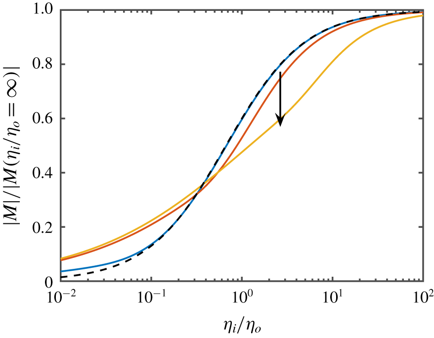
 $$\begin{eqnarray}M=\frac{V}{E}=M_{S}\frac{\displaystyle \frac{\unicode[STIX]{x1D702}_{i}}{\unicode[STIX]{x1D702}_{o}}}{\displaystyle \frac{\unicode[STIX]{x1D702}_{i}}{\unicode[STIX]{x1D702}_{o}}+\frac{2}{3}}\quad (|\unicode[STIX]{x1D701}|\ll k_{B}T/e,~\unicode[STIX]{x1D705}a\gg 1),\end{eqnarray}$$
where  $M_{S}=\unicode[STIX]{x1D716}_{o}\unicode[STIX]{x1D716}_{0}\unicode[STIX]{x1D701}/\unicode[STIX]{x1D702}_{o}$ is the Smoluchowski mobility (for a rigid sphere),
 $\unicode[STIX]{x1D702}_{i}/\unicode[STIX]{x1D702}_{o}$ is the ratio of the inside and outside shear viscosities, and
 $\unicode[STIX]{x1D716}_{o}\unicode[STIX]{x1D716}_{0}$ is the dielectric permittivity of the (outside) electrolyte. Note that the finite viscosity of the internal fluid decreases the mobility with respect to a rigid sphere, whereas the mobility of mercury drops is generally much higher than for their rigid-particle counterparts (Ohshima et al. Reference Ohshima, Healy and White1984; Schnitzer et al. Reference Schnitzer, Frankel and Yariv2013). However, as highlighted by Baygents & Saville (Reference Baygents and Saville1991a), surface-active impurities generate Marangoni stresses that suppress internal flow, thus making drops behave as rigid spheres (Velarde Reference Velarde1998). The numerical calculations of Baygents & Saville, undertaken in a similar manner to O’Brien & White (Reference O’Brien and White1978) for rigid spheres, reveal a wide variety of electrokinetic behaviours stemming from a greatly extended parameter space. Note that Baygents & Saville (Reference Baygents and Saville1991a) assume local equilibrium (captured as a proportionality) between the ions adsorbed at the interface and those in the fluid immediately adjacent to the interface, which produces the accompanying Marangoni stress. Baygents & Saville (Reference Baygents and Saville1991b) extend this model to weak electrolytes; and Schnitzer, Frankel & Yariv (Reference Schnitzer, Frankel and Yariv2014) have analysed in the strong-field limit for bubbles (without surface impurities), elucidating the special limit in which the measure of double-layer thickness is smaller than the measure of the electric field strength (when both are small). Despite these (and other) studies, Wuzhang et al. (Reference Wuzhang, Song, Sun, Pan and Li2015) have emphasized the need to know much more of how adsorbed charges on oil drops influence their electrophoretic mobility and flow.
In light-scattering and electrokinetic-sonic-amplitude (ESA) electrophoresis instruments, particles are subjected to oscillatory electric fields. The frequencies at which the electric field switches in light-scattering instruments seems to be less than  $100~\text{Hz}$, whereas ESA measures spectra in the range
 $1$–
 $20~\text{MHz}$. O’Brien (Reference O’Brien1988) pioneered the theoretical interpretation of ESA spectra, establishing how the measured oscillating acoustic pressure is related to the dynamic (frequency-dependent) electrophoretic mobility of rigid particles. He and others have developed theoretical formulae and computational models to connect the mobility to particle and electrolyte properties (O’Brien Reference O’Brien1986; Mangelsdorf & White Reference Mangelsdorf and White1992; Ohshima Reference Ohshima1996), thus providing a rigorous framework for converting the measured mobility spectrum to a
 $\unicode[STIX]{x1D701}$-potential. Noteworthy is that the ESA measurement does not require a dispersion to be optically transparent, so the mobility can be measured without dilution. Moreover, the magnitude and phase of dynamic mobility spectra can be used to ascertain the particle size and charge from one sample and measurement (O’Brien, Cannon & Rowlands Reference O’Brien, Cannon and Rowlands1995). We note that Mohammadi (Reference Mohammadi2016) has undertaken an impressive analytical calculation of the dynamic displacement of drops that are embedded in charged hydrogel media and subjected to an oscillatory electric field, albeit for low
 $\unicode[STIX]{x1D701}$-potentials without Marangoni effects. In principle, his formulae furnish the dynamic electrophoretic mobility of uniform and weakly charged drops in a Newtonian electrolyte.
Several electroacoustic measurements have been reported for surfactant-stabilized emulsions without drawing on a fluid-sphere model. Based on reasonable correspondence between fits of the rigid-sphere theory to data, one may question whether a dynamic fluid model is necessary. We believe that fluid characteristics could be concealed by the rigid-sphere model being fitted to ESA spectra with (i) an adjustable particle size distribution (e.g. log-normal), and (ii) a modified surface conductivity, which accounts for an additional surface-charge transport behind the shear plane (Djerdjev & Beattie Reference Djerdjev and Beattie2008). Evidently, both of these are necessary to satisfactorily fit to the data. According to this methodology, Djerdjev & Beattie (Reference Djerdjev and Beattie2008) have shown that the additional surface conductance is comparable to that of the diffuse layer. However, this suggests that adsorbed charge (behind the shear plane) has a mobility that is comparable to that of the counterions in the diffuse layer. It is not clear that this is physically acceptable, because surfactant molecules (e.g. dodecylsulfate, DS $^{-}$) are considerably larger than their (sodium, Na
 $^{+}$) counterions (Stigter Reference Stigter1967), and they reside predominantly in an oil phase (e.g. hexadecane) that has a viscosity higher than or comparable to that of water.
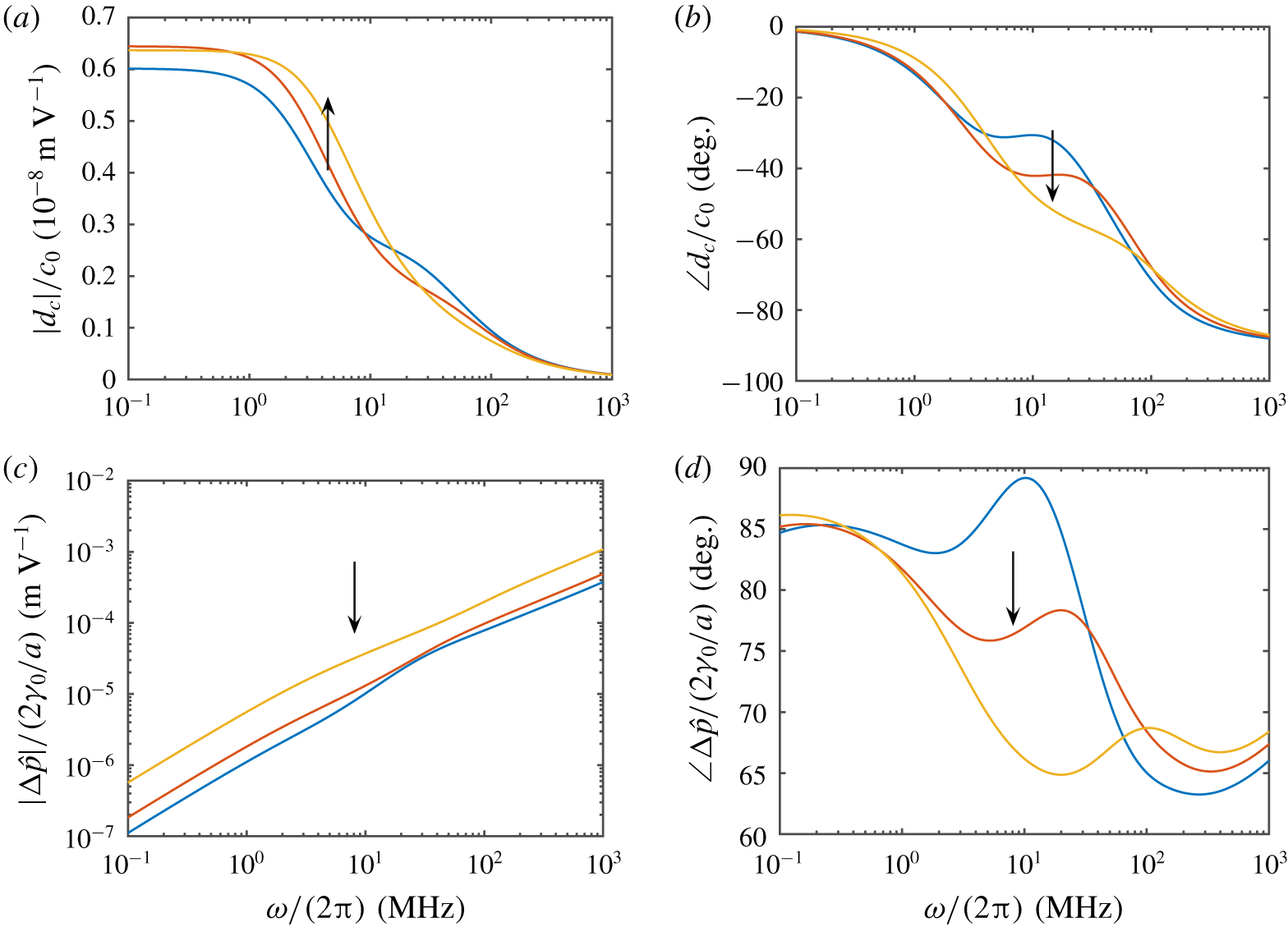
A theory to address the foregoing questions is set out as follows. After defining the general problem and basic assumptions (§ 2), we detail the general solution of a predominantly hydrodynamic problem for the flow in the bulk regions inside and outside a drop (§ 2.1). Next, we address the thin interfacial region where species, charge and momentum conservation principles are coupled, providing boundary conditions (matching conditions) for the two bulk regions (§§ 2.2 and 2.3). This model for the dynamics requires as input detailed knowledge of the equilibrium state of the interface, which is addressed separately by integrating the Gibbs thermodynamic relationship between surface tension and surface excesses (§ 2.4). Here, knowledge of the interfacial tension also furnishes the surface-charge density and, therefore, the equilibrium structure of the diffuse double layer. The results (§ 3) are presented by first interpreting the dynamic drag force (§ 3.1) and how it depends on the key dimensionless parameters, particularly the Marangoni number and ratio of concentration and momentum diffusivities. We then examine the dynamic mobility (§ 3.2), highlighting how the Marangoni effects manifest at the megahertz frequencies of ESA measurements. The paper concludes with a summary of the key results (§ 4).
2 Theory
We consider a dilute dispersion of oil drops in an aqueous electrolyte. It is assumed that a surfactant in the aqueous phase establishes an equilibrium partitioning between the aqueous phase and the oil–water interface, according to an isotherm derived from the concentration dependence of the surface tension of macroscopic, i.e. millimetre-sized drops. We will assume, for simplicity, that the dispersion is monodisperse with drop radius  $a$ and volume fraction
 $\unicode[STIX]{x1D719}$. Note that the size cannot be established from thermodynamics, which favours coalescence leading to macroscopic phase separation. However, the surface-charge density arising from the adsorption of an anionic surfactant tends to provide a strong electrosteric barrier to coalescence. Strong ultrasonic and/or mechanical mixing therefore produces emulsions with drop radii of several hundred nanometres. Thus, with a prescribed
 $\unicode[STIX]{x1D719}$ and measured
 $a$, an adsorption isotherm and prescribed total surfactant concentration
 $c_{\infty ,0}$ furnish the equilibrium interface
 $c^{0}$ (contributing to the total ‘surface excess’, number per unit area) and aqueous-phase
 $c_{\infty }$ surfactant concentrations. Accompanying this equilibrium state is an electrostatic surface potential
 $\unicode[STIX]{x1D701}$ and an equilibrium diffuse layer, which – at the high prevailing interfacial charge densities
 $zec^{0}$ – is predominantly occupied by ions with oppositely signed charge to the adsorbed surfactant.
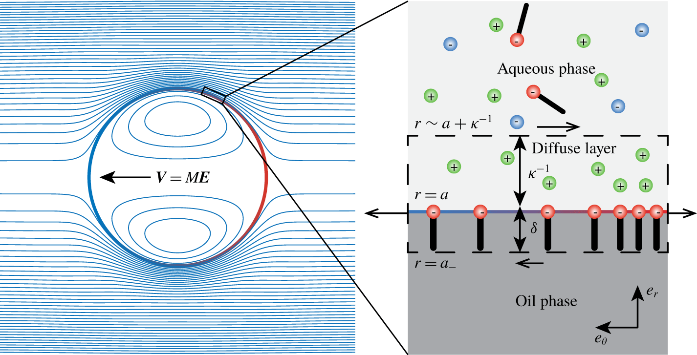
Schematic representation (not to scale) of a surfactant-stabilized nano-drop (of radius  $a$) subjected to an oscillatory electric field
 $\boldsymbol{E}\text{e}^{-\text{i}\unicode[STIX]{x1D714}t}$. The model is developed for
 $\unicode[STIX]{x1D6FF}\ll \unicode[STIX]{x1D705}^{-1}\ll a$ with no transfer of surfactant between the phases. The bulk surfactant (e.g. anionic SDS) concentration is below the c.m.c., with an interface concentration that is subject to lateral advection, diffusion and electromigration. The interfacial control volume (dashed lines) encloses the interface and diffuse layer, and so is electrically neutral: open arrows indicate the surface tractions: viscous on the top and bottom, and Marangoni/surface tension on the sides.

To probe the surface charge experimentally, such a dispersion may be subjected to an oscillatory electric field, represented mathematically as (the real part of)  $\boldsymbol{E}\text{e}^{-\text{i}\unicode[STIX]{x1D714}t}$. As is well known, this sets the particles into harmonic motion with a particle velocity
 $\boldsymbol{V}\text{e}^{-\text{i}\unicode[STIX]{x1D714}t}$, where
 $\boldsymbol{V}=M\boldsymbol{E}$ defines the (dynamic) electrophoretic mobility
 $M$. The electrokinetic model developed here seeks to ascertain how
 $M$ depends on the frequency
 $\unicode[STIX]{x1D714}/(2\unicode[STIX]{x03C0})$ and physical properties of the emulsion. As highlighted by the schematic in figure 1, the model is limited to drops for which the radius
 $a=O(10^{2})~\text{nm}$ is large compared to the characteristic thickness of the interface
 $\unicode[STIX]{x1D6FF}\lesssim O(1)~\text{nm}$ (assumed ideal, locally planar) and of the diffuse layer of counterions
 $\unicode[STIX]{x1D705}^{-1}<O(10)~\text{nm}$. The small (‘nanometric’) radius also makes the Laplace pressure sufficiently large to maintain a spherical shape when subjected to the electric field.
The present theory also assumes that there is no transfer of surfactant between the bulk solution and interface when responding to the electric field. This is motivated by the high frequencies encountered in ESA experiments, assuming that first-order kinetic rates (rate constants for adsorption and desorption,  $k_{a}$ and
 $k_{d}$) are much smaller than
 $\unicode[STIX]{x1D714}/(2\unicode[STIX]{x03C0})\sim 10^{6}~\text{Hz}$. Note that, with an equilibrium isotherm, only one of these kinetic rate constants is independent, since, at equilibrium,
 $c^{0}k_{d}=k_{a}c(r=a)$, where
 $c^{0}$ is the equilibrium surfactant (e.g. dodecylsulfate, DS
 $^{-}$, with valence
 $z=-1$) surface concentration and
 $c(r=a)=c_{\infty }\text{e}^{-z\unicode[STIX]{x1D701}e/k_{B}T}$ is the equilibrium surfactant concentration in the immediately adjacent electrolyte. Here,
 $c_{\infty }$ is the bulk surfactant concentration, and
 $\unicode[STIX]{x1D701}e/k_{B}T$ is the scaled equilibrium surface potential. It follows that (Denbigh Reference Denbigh1964)
 $$\begin{eqnarray}c^{0}=\frac{k_{a}}{k_{d}}c_{\infty }\text{e}^{-z\unicode[STIX]{x1D701}e/k_{B}T}=\hat{\unicode[STIX]{x1D6E4}}(c_{\infty },I_{s}),\end{eqnarray}$$
where  $\hat{\unicode[STIX]{x1D6E4}}(c_{\infty },I_{s})$ is an experimentally measurable function of the bulk surfactant concentration and the ionic strength of an added (non-adsorbing) salt (e.g. NaCl). In § 2.4, we present details of a theory that links a Langmuir model for the isotherm
 $\hat{\unicode[STIX]{x1D6E4}}(c_{\infty },I_{s})$ to the measurable interfacial surface tension
 $\unicode[STIX]{x1D6FE}^{0}(c_{\infty },I_{s})$. Note that a Langmuir isotherm at low bulk surfactant concentrations is proportional to
 $c_{\infty }$ with
 $|\unicode[STIX]{x1D701}|e/k_{B}T\ll 1$, in which case (2.1) furnishes
 $k_{a}/k_{d}=\text{const.}$, as adopted by Baygents & Saville (Reference Baygents and Saville1991a).
The subsections below address inner (drop), outer (bulk electrolyte) and interfacial (interface and diffuse layer) regions. The interfacial analysis (§ 2.2) provides boundary conditions that are necessary to match the inner and outer domains (§ 2.1). Note that, whereas the interfacial region may be considered an ‘inner’ boundary layer when adopting the language of matched asymptotic expansions, we use the terms ‘inner’ and ‘outer’ here to distinguish the bulk regions inside and outside the drop (both considered ‘outer’ in the context of matched asymptotic expansions). Our entire analysis implicitly tackles the leading-order matching due to  $\unicode[STIX]{x1D705}^{-1}\ll a$. We will also require the frequency to be sufficiently high that dynamic disturbances to the electrolyte composition are confined to the interfacial region. As described by Hunter (Reference Hunter2001), this requires
 $\sqrt{D_{i}/\unicode[STIX]{x1D714}}\lesssim a$, where
 $D_{i}\sim 10^{-9}~\text{m}^{2}~\text{s}^{-1}$ is an ionic diffusivity, so
 $\sqrt{\unicode[STIX]{x1D714}a^{2}/D_{i}}\gtrsim 1$. Supplementing the analysis of dynamics (which are taken to be linear perturbations to an equilibrium state) and dynamic mobility (§§ 2.1–2.3) is an analysis of the equilibrium interfacial thermodynamics (§ 2.4). This links the equilibrium surface tension and surface-charge density to the bulk composition. Readers who wish to skip the theoretical derivations may proceed to the final results (e.g. closed-form formulae available as (3.1), (3.2) and (3.3)) and discussion in § 3.
2.1 Bulk inner and outer regions
The bulk oil and aqueous phase beyond the diffuse layer are electrically neutral, and so their dynamics are governed by the unsteady Stokes equations ( $Re=Va/\unicode[STIX]{x1D708}\ll 1$)
 $$\begin{eqnarray}-\text{i}\unicode[STIX]{x1D714}\unicode[STIX]{x1D70C}\boldsymbol{u}=-\unicode[STIX]{x1D735}p+\unicode[STIX]{x1D702}\unicode[STIX]{x1D6FB}^{2}\boldsymbol{u}\quad \text{with }\unicode[STIX]{x1D735}\boldsymbol{\cdot }\boldsymbol{u}=0,\end{eqnarray}$$
where the density  $\unicode[STIX]{x1D70C}$ and shear viscosity
 $\unicode[STIX]{x1D702}$ (kinematic viscosity
 $\unicode[STIX]{x1D708}=\unicode[STIX]{x1D702}/\unicode[STIX]{x1D70C}$) for the oil and aqueous phases are hereafter distinguished using subscripts
 $i$ and
 $o$ (denoting inside and outside the drop) when appropriate. With the velocity
 $V\sim ME\sim 10^{-5}~\text{m}~\text{s}^{-1}$ (taking
 $M\sim 10^{-8}~\text{m}^{2}~\text{s}^{-1}~\text{V}^{-1}$ with
 $E\sim 10^{3}~\text{V}~\text{m}^{-1}$) and
 $\unicode[STIX]{x1D708}\sim 10^{-6}~\text{m}^{2}~\text{s}^{-1}$, a small Reynolds number is readily achieved for submicrometre-sized drops. Moreover, drops may be considered spherical, since the Laplace pressure dominates the inertial stress: balancing an
 $O(\unicode[STIX]{x1D714}\unicode[STIX]{x1D70C}Va)$ inertial stress with an
 $O(\unicode[STIX]{x1D6FE}/a)$ Laplace pressure (interfacial tension
 $\unicode[STIX]{x1D6FE}\sim 0.01~\text{N}~\text{m}^{-1}$) suggests a spherical interface when
 $a\lesssim \sqrt{\unicode[STIX]{x1D6FE}_{0}/(\unicode[STIX]{x1D714}\unicode[STIX]{x1D70C}_{o}ME)}\sim 1~\text{cm}$ with
 $\unicode[STIX]{x1D714}/(2\unicode[STIX]{x03C0})\sim 1~\text{kHz}$.
Symmetry, linearity and incompressibility demand solutions of the form
 $$\begin{eqnarray}\boldsymbol{u}=\unicode[STIX]{x1D735}\times [f(r)\boldsymbol{X}\times \boldsymbol{e}_{r}]=(f_{r}+fr^{-1})\boldsymbol{X}+(-f_{r}+fr^{-1})\boldsymbol{X}\boldsymbol{\cdot }\boldsymbol{e}_{r}\boldsymbol{e}_{r},\end{eqnarray}$$
with
 $$\begin{eqnarray}p=\hat{p}(r)\boldsymbol{X}\boldsymbol{\cdot }\boldsymbol{e}_{r},\end{eqnarray}$$
where  $\boldsymbol{X}=\boldsymbol{U}$ or
 $\boldsymbol{E}$, and
 $\boldsymbol{e}_{r}$ is a radial unit vector with
 $\boldsymbol{e}_{\unicode[STIX]{x1D703}}$ its tangential counterpart.
For mathematical convenience, we consider solutions for a stationary sphere at the origin with either a far-field translation of the fluid  $\boldsymbol{U}$ with electric field
 $\boldsymbol{E}=0$ or a finite electric field
 $\boldsymbol{E}$ with stationary far-field fluid
 $\boldsymbol{U}=0$. These far-field boundary conditions define what are termed the
 $U$- and
 $E$-problems, and their linear superposition will be used to construct a solution that satisfies boundary conditions that are compatible with the particle equation of motion.
Substituting the fluid velocity (which is divergence-free) and pressure above into the Stokes equations requires
 $$\begin{eqnarray}\hat{p}=\text{i}\unicode[STIX]{x1D6FA}r^{2}(f_{r}r^{-1}+fr^{-2})+rf_{rrr}+3f_{rr}-2f_{r}r^{-1}+2fr^{-2},\end{eqnarray}$$
where  $\unicode[STIX]{x1D6FA}=\unicode[STIX]{x1D714}\unicode[STIX]{x1D70C}/\unicode[STIX]{x1D702}$ (square of the reciprocal viscous penetration depth). Note that the continuity equation furnishes
 $\unicode[STIX]{x1D6FB}^{2}p=0$, so
 $\hat{p}=Ar^{-2}+Br$, where
 $A$ and
 $B$ are constants that can be ascertained from (2.2).
The general solution, leading to (2.3) and (2.4) for  $f$ and (2.5) and (2.6) for
 $\hat{p}$ below, is found as follows. Taking the curl of the momentum equation gives
 $$\begin{eqnarray}-\text{i}\unicode[STIX]{x1D6FA}\mathscr{L}(f)=\mathscr{L}^{2}(f),\end{eqnarray}$$
where
 $$\begin{eqnarray}\mathscr{L}=\frac{\unicode[STIX]{x2202}^{2}}{\unicode[STIX]{x2202}r^{2}}+\frac{2}{r}\frac{\unicode[STIX]{x2202}}{\unicode[STIX]{x2202}r}-\frac{2}{r^{2}}.\end{eqnarray}$$
Defining
 $$\begin{eqnarray}g=\mathscr{L}(f)\end{eqnarray}$$
gives
 $$\begin{eqnarray}-\text{i}\unicode[STIX]{x1D6FA}g=g_{rr}+2g_{r}/2-2g/r^{2},\end{eqnarray}$$
for which
 $$\begin{eqnarray}g=c_{2}\text{y}_{1}(\sqrt[4]{-1}\sqrt{\unicode[STIX]{x1D6FA}}r)-c_{1}\text{j}_{1}(\sqrt[4]{-1}\sqrt{\unicode[STIX]{x1D6FA}}r)\end{eqnarray}$$
and
 $$\begin{eqnarray}f_{rr}+2f_{r}/r-2f/r^{2}=g.\end{eqnarray}$$
The solution of this equation (in which  $\text{y}_{1}$ and
 $\text{j}_{1}$ are spherical Bessel functions) has four integration constants for each domain (
 $c_{1}$–
 $c_{4}$,
 $c_{1}^{\prime }$–
 $c_{4}^{\prime }$).
However, in the inside domain, removing singularities at the origin, and requiring zero radial velocity at  $r=a$, furnish
 $$\begin{eqnarray}f=c_{4}^{\prime }r+c_{1}^{\prime }\frac{\sqrt[4]{-1}\sqrt{\unicode[STIX]{x1D6FA}_{i}}r\cos (\sqrt[4]{-1}\sqrt{\unicode[STIX]{x1D6FA}_{i}}r)-\text{sin}(\sqrt[4]{-1}\sqrt{\unicode[STIX]{x1D6FA}_{i}}r)}{\unicode[STIX]{x1D6FA}_{i}^{2}r^{2}}\quad \text{for }r<a,\end{eqnarray}$$
where
 $$\begin{eqnarray}c_{4}^{\prime }=c_{1}^{\prime }a\frac{\sin (\sqrt[4]{-1}\sqrt{\unicode[STIX]{x1D6FA}_{i}}a)-\sqrt[4]{-1}\sqrt{\unicode[STIX]{x1D6FA}_{i}}a\cos (\sqrt[4]{-1}\sqrt{\unicode[STIX]{x1D6FA}_{i}}a)}{\unicode[STIX]{x1D6FA}_{i}^{2}a^{4}}.\end{eqnarray}$$
Similarly, in the outside domain, removing singularities in the far field and requiring zero radial velocity as  $r\rightarrow a$, furnish
 $$\begin{eqnarray}f=\frac{U}{2X}r+c_{3}r^{-2}+c_{1}\frac{(\sqrt[4]{-1}\sqrt{\unicode[STIX]{x1D6FA}_{o}}r+\text{i})\text{e}^{(\text{i}-1)\sqrt{\unicode[STIX]{x1D6FA}_{o}/2}r}}{\unicode[STIX]{x1D6FA}_{o}^{2}r^{2}}\quad \text{for }r>a,\end{eqnarray}$$
where
 $$\begin{eqnarray}c_{3}=-\frac{U}{2X}a^{3}-c_{1}a\frac{(\sqrt[4]{-1}\sqrt{\unicode[STIX]{x1D6FA}_{o}}a+\text{i})\text{e}^{(\text{i}-1)\sqrt{\unicode[STIX]{x1D6FA}_{o}/2}a}}{\unicode[STIX]{x1D6FA}_{o}^{2}a}.\end{eqnarray}$$
The inner and outer flows are therefore determined to within one unknown scalar coefficient each:  $c_{1}^{\prime }$ and
 $c_{1}$. We will prescribe these using boundary conditions arising from analysis of the interfacial region, as undertaken in § 2.2 below. Similarly to the fluid properties, subscripts
 $i$ and
 $o$ attached to
 $\unicode[STIX]{x1D6FA}$ denote inside and outside the drop.
With the entire fluid velocity (outside the interfacial region) now prescribed by just two scalar constants of integration, equation (2.2) furnishes
 $$\begin{eqnarray}\hat{p}=-{\textstyle \frac{2}{3}}\sqrt[4]{-1}\sqrt{\unicode[STIX]{x1D6FA}_{i}}c_{1}^{\prime }r\quad \text{for }r<a\end{eqnarray}$$
and
 $$\begin{eqnarray}\hat{p}=\text{i}\unicode[STIX]{x1D6FA}_{o}\left(\frac{U}{X}r-c_{3}r^{-2}\right)\quad \text{for }r>a.\end{eqnarray}$$
These confirm that  $p$ satisfies Laplace’s equation. Note that
 $\unicode[STIX]{x1D6FA}$ and the integration constants must be prescribed separately for the inside and outside domains, which are coupled by boundary conditions at
 $r=a$ that account for electro-osmotic and Marangoni flow in the interfacial region. For future reference, note that the tangential velocity
 $\boldsymbol{u}_{\unicode[STIX]{x1D703}}$ and traction
 $\boldsymbol{t}_{\unicode[STIX]{x1D703}}$ (on the surface with inward unit normal
 $-\boldsymbol{e}_{r}$) inside the interface (i.e. at the interface, on the drop side,
 $r=a_{-}$) are
 $$\begin{eqnarray}\boldsymbol{u}_{\unicode[STIX]{x1D703}}(r=a_{-})=f_{r}\boldsymbol{X}\boldsymbol{\cdot }\boldsymbol{e}_{\unicode[STIX]{x1D703}}\boldsymbol{e}_{\unicode[STIX]{x1D703}}=c_{1}^{\prime }aV_{i}(\unicode[STIX]{x1D6FA}_{i}a^{2})\boldsymbol{X}\boldsymbol{\cdot }\boldsymbol{e}_{\unicode[STIX]{x1D703}}\boldsymbol{e}_{\unicode[STIX]{x1D703}},\end{eqnarray}$$
where
 $$\begin{eqnarray}V_{i}(\unicode[STIX]{x1D6FA}_{i}a^{2})=\frac{(3-\text{i}\unicode[STIX]{x1D6FA}_{i}a^{2})\sin (\sqrt[4]{-1}\sqrt{\unicode[STIX]{x1D6FA}_{i}}a)-3\sqrt[4]{-1}\sqrt{\unicode[STIX]{x1D6FA}_{i}}a\cos (\sqrt[4]{-1}\sqrt{\unicode[STIX]{x1D6FA}_{i}}a)}{\unicode[STIX]{x1D6FA}_{i}^{2}a^{4}}\end{eqnarray}$$
and
 $$\begin{eqnarray}\boldsymbol{t}_{\unicode[STIX]{x1D703}}(r=a_{-})=-\unicode[STIX]{x1D702}_{i}f_{rr}(a)\boldsymbol{X}\boldsymbol{\cdot }\boldsymbol{e}_{\unicode[STIX]{x1D703}}\boldsymbol{e}_{\unicode[STIX]{x1D703}}=-\unicode[STIX]{x1D702}_{i}c_{1}^{\prime }T_{i}(\unicode[STIX]{x1D6FA}_{i}a^{2})\boldsymbol{X}\boldsymbol{\cdot }\boldsymbol{e}_{\unicode[STIX]{x1D703}}\boldsymbol{e}_{\unicode[STIX]{x1D703}},\end{eqnarray}$$
where
 $$\begin{eqnarray}\displaystyle & & \displaystyle \hspace{-9.60004pt}T_{i}(\unicode[STIX]{x1D6FA}_{i}a^{2})\nonumber\\ \displaystyle & & \displaystyle \quad =\frac{(6\sqrt[4]{-1}\sqrt{\unicode[STIX]{x1D6FA}_{i}}a-(-1)^{3/4}\unicode[STIX]{x1D6FA}_{i}^{3/2}a^{3})\cos (\sqrt[4]{-1}\sqrt{\unicode[STIX]{x1D6FA}_{i}}a)+(3\text{i}\unicode[STIX]{x1D6FA}_{i}a^{2}-6)\sin (\sqrt[4]{-1}\sqrt{\unicode[STIX]{x1D6FA}_{i}}a)}{\unicode[STIX]{x1D6FA}_{i}^{2}a^{4}}.\nonumber\\ \displaystyle & & \displaystyle\end{eqnarray}$$
Outside the interface (i.e. at the interface, on the aqueous side,  $r=a_{+}$), the tangential velocity and traction (surface with outward unit normal
 $\boldsymbol{e}_{r}$) are
 $$\begin{eqnarray}\boldsymbol{u}_{\unicode[STIX]{x1D703}}(r=a_{+})=f_{r}\boldsymbol{X}\boldsymbol{\cdot }\boldsymbol{e}_{\unicode[STIX]{x1D703}}\boldsymbol{e}_{\unicode[STIX]{x1D703}}\quad \text{and}\quad \boldsymbol{t}_{\unicode[STIX]{x1D703}}(r=a_{+})=\unicode[STIX]{x1D702}_{o}f_{rr}\boldsymbol{X}\boldsymbol{\cdot }\boldsymbol{e}_{\unicode[STIX]{x1D703}}\boldsymbol{e}_{\unicode[STIX]{x1D703}},\end{eqnarray}$$
where
 $$\begin{eqnarray}f_{r}(r=a_{+})=\frac{3U}{2X}-c_{1}aV_{o}(\unicode[STIX]{x1D6FA}_{o}a^{2})\end{eqnarray}$$
and
 $$\begin{eqnarray}f_{rr}(r=a_{+})=-\frac{3U}{Xa}+c_{1}T_{o}(\unicode[STIX]{x1D6FA}_{o}a^{2}),\end{eqnarray}$$
which define
 $$\begin{eqnarray}V_{o}(\unicode[STIX]{x1D6FA}_{o}a^{2})=\frac{\text{e}^{(\text{i}-1)\sqrt{\unicode[STIX]{x1D6FA}_{o}/2}a}}{\unicode[STIX]{x1D6FA}_{o}a^{2}}\end{eqnarray}$$
and
 $$\begin{eqnarray}T_{o}(\unicode[STIX]{x1D6FA}_{o}a^{2})=[3-(\text{i}-1)\sqrt{\unicode[STIX]{x1D6FA}_{o}/2}a]V_{o}(\unicode[STIX]{x1D6FA}_{o}a^{2}).\end{eqnarray}$$
The coefficient  $c_{3}$ for the outside flow measures the (dipole) strength of the decaying contribution to the pressure, which also measures the slowest-decaying contribution to the velocity disturbance, e.g. as identified in (2.4). Note that integrating the total hydrodynamic traction over the surface of a sphere furnishes a force
 $$\begin{eqnarray}\boldsymbol{F}(r=a_{+})=-{\textstyle \frac{4}{3}}\unicode[STIX]{x03C0}a^{2}\unicode[STIX]{x1D702}_{o}\boldsymbol{X}[\text{i}\unicode[STIX]{x1D6FA}_{o}(rf_{r}+f)+rf_{rrr}+f_{rr}-6f_{r}r^{-1}+6fr^{-2}],\end{eqnarray}$$
where the terms premultiplied by  $\text{i}\unicode[STIX]{x1D6FA}_{o}$ come from the pressure/normal traction. This formula does not include the electrical stress, which is non-zero on the surface of the drop. This physics enters via the interfacial region and its coupling to the outer flows, as addressed in § 2.2 below. A much more convenient evaluation of the force is available that requires only knowledge of
 $c_{3}$ (measuring the far-field decay of the outer velocity disturbance), furnishing (Mangelsdorf & White Reference Mangelsdorf and White1992)
 $$\begin{eqnarray}\boldsymbol{F}=6\unicode[STIX]{x03C0}\unicode[STIX]{x1D702}_{o}a\boldsymbol{X}{\textstyle \frac{2}{3}}\text{i}\unicode[STIX]{x1D6FA}_{o}a^{2}c_{3}a^{-3}.\end{eqnarray}$$
Accompanying the foregoing hydrodynamic flows is an electrostatic potential  $\unicode[STIX]{x1D713}^{\prime }$, which can be shown (at sufficiently high frequency) to satisfy Laplace’s equation everywhere, i.e. in the bulk and interfacial regions:
 $$\begin{eqnarray}\unicode[STIX]{x1D6FB}^{2}\unicode[STIX]{x1D713}^{\prime }=0.\end{eqnarray}$$
Thus, linearity, symmetry and the far field require
 $$\begin{eqnarray}\unicode[STIX]{x1D713}^{\prime }=r[-(E/X)+\hat{d}_{\unicode[STIX]{x1D713}}r^{-3}]\boldsymbol{X}\boldsymbol{\cdot }\boldsymbol{e}_{r}\quad \text{for }r>a,\end{eqnarray}$$
where we will term  $\hat{d}_{\unicode[STIX]{x1D713}}$ the (electrostatic) dipole strength. This measures electrical polarization of the interfacial region, which has contributions from the charge-density perturbations in the diffuse layer and at the interface due to lateral transport of charged surfactant. To be finite inside the drop and continuous across the interface (continuous tangential electric field (Baygents & Saville Reference Baygents and Saville1991a)), the potential inside the drop must be
 $$\begin{eqnarray}\unicode[STIX]{x1D713}^{\prime }=r[-(E/X)+\hat{d}_{\unicode[STIX]{x1D713}}a^{-3}]\boldsymbol{X}\boldsymbol{\cdot }\boldsymbol{e}_{r}\quad \text{for }r<a.\end{eqnarray}$$
Perturbations to the equilibrium interfacial charge and momentum balances are addressed below: together, these determine the presently unknown scalars,  $\hat{d}_{\unicode[STIX]{x1D713}}$,
 $c_{1}$ and
 $c_{1}^{\prime }$ (and therefore
 $c_{3}$).
2.2 Inner/interfacial region
This inner region provides matching conditions for the foregoing solutions in the bulk regions. Here, in addition to mass and momentum conservation, we must consider the conservation of ions and surfactant molecules in the aqueous phase, and of surfactant molecules adsorbed on the interface. These differential relationships are coupled, and we will show that their solution leads to a set of linear algebraic relationships which, when combined with those in § 2.1, solve the full dynamic electrokinetic model.
We begin with a species conservation equation for any molecular species (subscript  $i$) that is subject to advection, diffusion and electromigration:
 $$\begin{eqnarray}-\unicode[STIX]{x1D735}\boldsymbol{\cdot }\,\boldsymbol{j}_{i}=-\text{i}\unicode[STIX]{x1D714}c_{i}^{\prime }\quad \text{with }\boldsymbol{j}_{i}=-D_{i}\unicode[STIX]{x1D735}c_{i}^{\prime }-\unicode[STIX]{x1D735}\unicode[STIX]{x1D713}^{0}z_{i}ec_{i}^{\prime }\frac{D_{i}}{k_{B}T}-\unicode[STIX]{x1D735}\unicode[STIX]{x1D713}^{\prime }z_{i}ec_{i}^{0}\frac{D_{i}}{k_{B}T}+\boldsymbol{u}c_{i}^{0}.\end{eqnarray}$$
Note that we have linearized the flux with respect to perturbations defined by  $c_{i}=c_{i}^{0}+c_{i}^{\prime }$ and
 $\unicode[STIX]{x1D713}=\unicode[STIX]{x1D713}^{0}+\unicode[STIX]{x1D713}^{\prime }$, where
 $c_{i}$ denotes the concentration of a species with
 $c_{i}^{0}$ the equilibrium concentration, and
 $c_{i}^{\prime }$ the perturbation induced by the forcing
 $\boldsymbol{X}$.
Similarly,  $\unicode[STIX]{x1D713}^{0}$ and
 $\unicode[STIX]{x1D713}^{\prime }$ denote the equilibrium electrostatic potential and perturbation. As usual,
 $D_{i}$,
 $z_{i}$,
 $e$ and
 $k_{B}T$ are the diffusion coefficient, valence, fundamental charge and thermal energy. Note that the equilibrium quantities are functions of radial position, for which tangential gradients vanish in the formulae below. As is well known, the equilibrium state satisfies the nonlinear Poisson–Boltzmann equation (Russel et al. Reference Russel, Saville and Showalter1989):
 $$\begin{eqnarray}\unicode[STIX]{x1D716}\unicode[STIX]{x1D716}_{0}\unicode[STIX]{x1D6FB}^{2}\unicode[STIX]{x1D713}^{0}(r)=-\mathop{\sum }_{i}z_{i}ec_{i}^{0}(r),\end{eqnarray}$$
where ( $\unicode[STIX]{x1D716}\unicode[STIX]{x1D716}_{0}$ is the dielectric permittivity)
 $$\begin{eqnarray}c_{i}^{0}(r)=c_{i}^{\infty }\text{e}^{-\unicode[STIX]{x1D713}^{0}(r)z_{i}e/k_{B}T}.\end{eqnarray}$$
The radial and tangential components of  $\boldsymbol{j}_{i}$ are
 $$\begin{eqnarray}\boldsymbol{j}_{i,r}=\left[-D_{i}\unicode[STIX]{x1D735}c_{i}^{\prime }-\unicode[STIX]{x1D735}\unicode[STIX]{x1D713}^{0}z_{i}ec_{i}^{\prime }\frac{D_{i}}{k_{B}T}-\unicode[STIX]{x1D735}\unicode[STIX]{x1D713}^{\prime }z_{i}ec_{i}^{0}\frac{D_{i}}{k_{B}T}+\boldsymbol{u}c_{i}^{0}\right]\boldsymbol{\cdot }\boldsymbol{e}_{r}\boldsymbol{e}_{r}\end{eqnarray}$$
and
 $$\begin{eqnarray}\boldsymbol{j}_{i,\unicode[STIX]{x1D703}}=\left[-D_{i}\unicode[STIX]{x1D735}c_{i}^{\prime }-\unicode[STIX]{x1D735}\unicode[STIX]{x1D713}^{\prime }z_{i}ec_{i}^{0}\frac{D_{i}}{k_{B}T}+\boldsymbol{u}c_{i}^{0}\right]\boldsymbol{\cdot }\boldsymbol{e}_{\unicode[STIX]{x1D703}}\boldsymbol{e}_{\unicode[STIX]{x1D703}}.\end{eqnarray}$$
These can be used to develop conservation equations for an interfacial control volume (thickness  ${\sim}\unicode[STIX]{x1D705}^{-1}\ll a$, as identified by the region bounded by dashed lines in figure 1):
 $$\begin{eqnarray}-\unicode[STIX]{x1D735}_{s}\boldsymbol{\cdot }\left\langle -D_{i}\unicode[STIX]{x1D735}_{s}c_{i}^{\prime }-\unicode[STIX]{x1D735}_{s}\unicode[STIX]{x1D713}^{\prime }z_{i}ec_{i}^{0}\frac{D_{i}}{k_{B}T}+\boldsymbol{u}_{\unicode[STIX]{x1D703}}c_{i}^{0}\right\rangle -\boldsymbol{j}_{r}\boldsymbol{\cdot }\boldsymbol{e}_{r}=\langle -\text{i}\unicode[STIX]{x1D714}c_{i}^{\prime }\rangle ,\end{eqnarray}$$
where  $\unicode[STIX]{x1D735}_{s}$ is the surface gradient operator,
 $\boldsymbol{u}_{\unicode[STIX]{x1D703}}=\boldsymbol{u}\boldsymbol{\cdot }\boldsymbol{e}_{\unicode[STIX]{x1D703}}\boldsymbol{e}_{\unicode[STIX]{x1D703}}$, and
 $$\begin{eqnarray}\langle \cdot \rangle =\int _{r^{\prime }=a}^{r}\cdot \,\text{d}r^{\prime }.\end{eqnarray}$$
Linearity and symmetry require the general forms
 $$\begin{eqnarray}c_{i}^{\prime }=d_{i,c}(r)\boldsymbol{X}\boldsymbol{\cdot }\boldsymbol{e}_{r}\quad \text{and}\quad \unicode[STIX]{x1D713}^{\prime }=d_{\unicode[STIX]{x1D713}}(r)\boldsymbol{X}\boldsymbol{\cdot }\boldsymbol{e}_{r},\end{eqnarray}$$
with
 $$\begin{eqnarray}\boldsymbol{u}_{r}=2fr^{-1}\boldsymbol{X}\boldsymbol{\cdot }\boldsymbol{e}_{r}\boldsymbol{e}_{r}\quad \text{and}\quad \boldsymbol{u}_{\unicode[STIX]{x1D703}}=(f_{r}+fr^{-1})\boldsymbol{X}\boldsymbol{\cdot }\boldsymbol{e}_{\unicode[STIX]{x1D703}}\boldsymbol{e}_{\unicode[STIX]{x1D703}}.\end{eqnarray}$$
Note that, within the diffuse layer, the function  $f$ here is not the one calculated in the section above (outer domain), since the momentum equation for the diffuse layer includes an electrical body force that drives electro-osmotic flow.
With the foregoing forms of the perturbation functions, the conservation equations (one for each species) for the diffuse layer become
 $$\begin{eqnarray}\left\langle 2r^{-2}(\text{i}\unicode[STIX]{x1D714}r^{2}/2-D_{i})d_{i,c}-2r^{-1}d_{\unicode[STIX]{x1D713}}z_{i}ec_{i}^{0}\frac{D_{i}}{k_{B}T}+2r^{-1}(f_{r}+fr^{-1})c_{i}^{0}\right\rangle \boldsymbol{X}\boldsymbol{\cdot }\boldsymbol{e}_{r}=\boldsymbol{j}_{i,r}\boldsymbol{\cdot }\boldsymbol{e}_{r},\end{eqnarray}$$
where
 $$\begin{eqnarray}\boldsymbol{j}_{i,r}\boldsymbol{\cdot }\boldsymbol{e}_{r}=\left[-D_{i}d_{i,c,r}-\unicode[STIX]{x1D713}_{r}^{0}z_{i}ed_{i,c}\frac{D_{i}}{k_{B}T}-d_{\unicode[STIX]{x1D713},r}z_{i}ec_{i}^{0}\frac{D_{i}}{k_{B}T}+2fr^{-1}c_{i}^{0}\right]\boldsymbol{X}\boldsymbol{\cdot }\boldsymbol{e}_{r}.\end{eqnarray}$$
Note that we have prescribed zero flux on the oil side of the oil–water interface, assuming that the integrals are finite when  $r\gtrsim a+\unicode[STIX]{x1D705}^{-1}=a_{+}$.
Applying (2.11) to the surfactant adsorbed on the interface (taking the thickness of the control volume to zero with a Dirac-delta concentration  $(c^{0}+c^{\prime })\unicode[STIX]{x1D6FF}(r-a)$), where (as required by linearity and symmetry)
 $$\begin{eqnarray}c^{\prime }=d_{c}\boldsymbol{X}\boldsymbol{\cdot }\boldsymbol{e}_{r}\end{eqnarray}$$
is the surface-concentration perturbation, gives
 $$\begin{eqnarray}(\text{i}\unicode[STIX]{x1D714}a^{2}/2-D)d_{c}-d_{\unicode[STIX]{x1D713}}zec^{0}\frac{D}{k_{B}T}+a(f_{r}+fa^{-1})c^{0}=0\quad \text{at }r=a,\end{eqnarray}$$
where the absence of a subscript  $i$ attached to
 $c^{\prime }$,
 $c^{0}$,
 $d_{c}$,
 $D$ and
 $z$ distinguishes the adsorbed surfactant from the non-adsorbed species; it follows that
 $c^{0}$ is now a surface concentration (molecules per unit area). Note that this balance captures tangential transport (electromigration, diffusion and advection) of the adsorbed surfactant, neglecting exchange with the oil and aqueous phases. Here, the approximation is motivated by the high frequency of the oscillating electric field. Thus, with diffusion-limited exchange kinetics, we anticipate an
 $O(D/a^{2})$ limit on the frequency below which the model may break down.
The constant  $d_{c}$ measures the concentration polarization of the interface, which is forced by advection and electromigration, and relaxed by diffusion. The surface divergence of the interface velocity is
 $$\begin{eqnarray}\unicode[STIX]{x1D735}_{s}\boldsymbol{\cdot }\boldsymbol{u}_{\unicode[STIX]{x1D703}}=-2a^{-1}(f_{r}+fa^{-1})\boldsymbol{X}\boldsymbol{\cdot }\boldsymbol{e}_{r}=-2a^{-1}c_{1}^{\prime }V_{i}(\unicode[STIX]{x1D6FA}_{i}a^{2})X\cos \unicode[STIX]{x1D703}.\end{eqnarray}$$
A charge conservation relationship for the interfacial control volume is obtained by multiplying the species conservation equations above by the respective charge  $z_{i}e$ and summing over all species:
 $$\begin{eqnarray}\displaystyle & & \displaystyle \mathop{\sum }_{i}\left\langle -2r^{-2}D_{i}d_{c,i}-2r^{-2}d_{\unicode[STIX]{x1D713}}z_{i}ec_{i}^{0}\frac{D_{i}}{k_{B}T}+2r^{-1}(f_{r}+fr^{-1})c_{i}^{0}\right\rangle z_{i}e\nonumber\\ \displaystyle & & \displaystyle \quad -\,\mathop{\sum }_{i}\left[-D_{i}d_{c,i,r}-\unicode[STIX]{x1D713}_{r}^{0}z_{i}ed_{c,i}\frac{D_{i}}{k_{B}T}-d_{\unicode[STIX]{x1D713},r}z_{i}ec_{i}^{0}\frac{D_{i}}{k_{B}T}+2fr^{-1}c_{i}^{0}\right]z_{i}e=-\text{i}\unicode[STIX]{x1D714}d_{\unicode[STIX]{x1D70E}},\qquad\end{eqnarray}$$
where
 $$\begin{eqnarray}d_{\unicode[STIX]{x1D70E}}=\mathop{\sum }_{i}z_{i}e\langle d_{c,i}\rangle\end{eqnarray}$$
measures the net charge density (per unit area). Recall that we have taken the radial flux of all species at  $r=a_{-}$ to be zero, so the second sum is to be evaluated at
 $r\sim a+\unicode[STIX]{x1D705}^{-1}=a_{+}$.
Similarly to the radially averaged species conservation equation above, the (perturbed) Poisson equation
 $$\begin{eqnarray}-\unicode[STIX]{x1D735}\boldsymbol{\cdot }(\unicode[STIX]{x1D716}\unicode[STIX]{x1D716}_{0}\unicode[STIX]{x1D735}\unicode[STIX]{x1D713}^{\prime })=\mathop{\sum }_{i}z_{i}ec_{i}^{\prime }\end{eqnarray}$$
may be written as
 $$\begin{eqnarray}-\unicode[STIX]{x1D716}_{o}\unicode[STIX]{x1D716}_{0}\unicode[STIX]{x1D735}\unicode[STIX]{x1D713}^{\prime }\boldsymbol{\cdot }\boldsymbol{e}_{r}|_{a_{+}}+\unicode[STIX]{x1D716}_{i}\unicode[STIX]{x1D716}_{0}\unicode[STIX]{x1D735}\unicode[STIX]{x1D713}^{\prime }\boldsymbol{\cdot }\boldsymbol{e}_{r}|_{a_{-}}-\unicode[STIX]{x1D716}_{o}\unicode[STIX]{x1D716}_{0}\unicode[STIX]{x1D6FB}_{s}^{2}\langle \unicode[STIX]{x1D713}^{\prime }\rangle =\mathop{\sum }_{i}z_{i}e\langle c_{i}^{\prime }\rangle ,\end{eqnarray}$$
which ( $\unicode[STIX]{x1D716}_{i}\unicode[STIX]{x1D716}_{0}$ and
 $\unicode[STIX]{x1D716}_{o}\unicode[STIX]{x1D716}_{0}$ are the dielectric permittivities of the inside (oil) and outside (aqueous) phases), using the foregoing forms of the perturbation functions, becomes
 $$\begin{eqnarray}-\unicode[STIX]{x1D716}_{o}\unicode[STIX]{x1D716}_{0}d_{\unicode[STIX]{x1D713},r}|_{a_{+}}+\unicode[STIX]{x1D716}_{i}\unicode[STIX]{x1D716}_{0}d_{\unicode[STIX]{x1D713},r}|_{a_{-}}+\unicode[STIX]{x1D716}_{o}\unicode[STIX]{x1D716}_{0}2a^{-2}\langle d_{\unicode[STIX]{x1D713}}\rangle =\mathop{\sum }_{i}z_{i}e\langle d_{c,i}\rangle =d_{\unicode[STIX]{x1D70E}}.\end{eqnarray}$$
We can now eliminate  $d_{\unicode[STIX]{x1D70E}}$ from the Poisson and charge-conservation equations (2.13) and (2.14), furnishing
 $$\begin{eqnarray}\displaystyle & & \displaystyle \text{i}\unicode[STIX]{x1D714}\unicode[STIX]{x1D716}_{o}\unicode[STIX]{x1D716}_{0}d_{\unicode[STIX]{x1D713},r}|_{a_{+}}-\text{i}\unicode[STIX]{x1D714}\unicode[STIX]{x1D716}_{i}\unicode[STIX]{x1D716}_{0}d_{\unicode[STIX]{x1D713},r}|_{a_{-}}+\unicode[STIX]{x1D716}_{o}\unicode[STIX]{x1D716}_{0}2a^{-2}\langle d_{\unicode[STIX]{x1D713}}\rangle \nonumber\\ \displaystyle & & \displaystyle \quad =\mathop{\sum }_{i}\left\langle -2r^{-2}D_{i}d_{c,i}-2r^{-2}d_{\unicode[STIX]{x1D713}}z_{i}ec_{i}^{0}\frac{D_{i}}{k_{B}T}+2r^{-1}(f_{r}+fr^{-1})c_{i}^{0}\right\rangle z_{i}e\nonumber\\ \displaystyle & & \displaystyle \qquad -\,\mathop{\sum }_{i}\left[-D_{i}d_{c,i,r}-\unicode[STIX]{x1D713}_{r}^{0}z_{i}ed_{c,i}\frac{D_{i}}{k_{B}T}-d_{\unicode[STIX]{x1D713},r}z_{i}ec_{i}^{0}\frac{D_{i}}{k_{B}T}+2fr^{-1}c_{i}^{0}\right]z_{i}e\nonumber\\ \displaystyle & & \displaystyle \qquad -\,2a^{-2}Dzed_{c}-2a^{-2}d_{\unicode[STIX]{x1D713}}(ze)^{2}c^{0}\frac{D}{k_{B}T}+2a^{-1}(f_{r}+fa^{-1})c^{0}ze.\end{eqnarray}$$
Note that sums are now over all mobile species in the diffuse layer, and the last line (tangential transport of the surfactant at the interface) is the separate contribution (to the interfacial charge balance from radial and tangential fluxes) of the adsorbed species at the interface with  $f$ (i.e. the advective velocity) evaluated at
 $r=a_{-}$ for the oil phase (where
 $f=0$ due to the radial velocity vanishing at the interface).
Next, based on a thin diffuse layer, we note that the third term on the left-hand side of (2.15) will be  $O(\unicode[STIX]{x1D705}^{-1}/a)$ smaller than the other terms, and may therefore be neglected. Moreover, O’Brien (Reference O’Brien1988) has analysed the other radial and tangential fluxes in the second and third lines of equation (2.15), for thin diffuse layers, showing that they can be expressed in terms of the ‘surface’ (hereafter termed ‘diffuse layer’) and bulk conductivities,
 $K_{s}$ and
 $K_{\infty }$, with the electrostatic potential inside the diffuse layer well approximated by the electrostatic potential in the outer domain, which satisfies Laplace’s equation. Note that O’Brien’s
 $K_{s}$ accounts for charge transport within the (thin) diffuse layer and its exchange with the outer bulk domain. Thus, drawing on his analysis of current in the diffuse layer, we set
 $$\begin{eqnarray}\displaystyle & & \displaystyle \mathop{\sum }_{i}\left\langle -2r^{-2}D_{i}d_{c,i}-2r^{-2}d_{\unicode[STIX]{x1D713}}z_{i}ec_{i}^{0}\frac{D_{i}}{k_{B}T}+2r^{-1}(f_{r}+fr^{-1})c_{i}^{0}\right\rangle z_{i}e\nonumber\\ \displaystyle & & \displaystyle \qquad -\,\mathop{\sum }_{i}\left[-D_{i}d_{c,i,r}-\unicode[STIX]{x1D713}_{r}^{0}z_{i}ed_{c,i}\frac{D_{i}}{k_{B}T}-d_{\unicode[STIX]{x1D713},r}z_{i}ec_{i}^{0}\frac{D_{i}}{k_{B}T}+2fr^{-1}c_{i}^{0}\right]z_{i}e\nonumber\\ \displaystyle & & \displaystyle \quad =2K_{s}a^{-1}(E/X-\hat{d}_{\unicode[STIX]{x1D713}}a^{-3})-K_{\infty }(E/X+2\hat{d}_{\unicode[STIX]{x1D713}}a^{-3})\nonumber\\ \displaystyle & & \displaystyle \qquad +\,2a^{-1}(f_{r}+fa^{-1})\mathop{\sum }_{i}\langle c_{i}^{0}\rangle z_{i}e-2fa^{-1}\mathop{\sum }_{i}c_{i}^{0}z_{i}e,\nonumber\end{eqnarray}$$
where we have used (§ 2.1)  $d_{\unicode[STIX]{x1D713}}(r=a_{+})=-a(E/X-\hat{d}_{\unicode[STIX]{x1D713}}a^{-3})$,
 $d_{\unicode[STIX]{x1D713},r}(r=a_{+})=-(E/X+2\hat{d}_{\unicode[STIX]{x1D713}}a^{-3})$ and
 $d_{\unicode[STIX]{x1D713},r}(r=a_{-})=-(E/X-\hat{d}_{\unicode[STIX]{x1D713}}a^{-3})$. Note that the last two terms capture the advective contribution to the current arising from the interfacial mobility. The first of these is the tangential velocity of the interface multiplied by the net charge of the diffuse layer, and the second is the radial velocity of the interface multiplied by the net (vanishing) charge outside the diffuse layer. From the boundary conditions in § 2.1, the only non-zero term is
 $$\begin{eqnarray}2a^{-1}f_{r}\mathop{\sum }_{i}\langle c_{i}^{0}\rangle z_{i}e=-2a^{-1}f_{r}c^{0}ze,\end{eqnarray}$$
which, by overall electroneutrality of the interfacial control volume (interface and diffuse layer), is equal and opposite to the advective current of the adsorbed species at the interface. Equation (2.15) therefore reduces to
 $$\begin{eqnarray}\displaystyle & & \displaystyle -\text{i}\unicode[STIX]{x1D714}\unicode[STIX]{x1D716}_{o}\unicode[STIX]{x1D716}_{0}(E/X+2\hat{d}_{\unicode[STIX]{x1D713}}a^{-3})+\text{i}\unicode[STIX]{x1D714}\unicode[STIX]{x1D716}_{i}\unicode[STIX]{x1D716}_{0}(E/X-\hat{d}_{\unicode[STIX]{x1D713}}a^{-3})\nonumber\\ \displaystyle & & \displaystyle \quad =2K_{s}a^{-1}(E/X-\hat{d}_{\unicode[STIX]{x1D713}}a^{-3})-K_{\infty }(E/X+2\hat{d}_{\unicode[STIX]{x1D713}}a^{-3})\nonumber\\ \displaystyle & & \displaystyle \qquad -\,2a^{-2}Dzed_{c}+2a^{-1}(E/X-\hat{d}_{\unicode[STIX]{x1D713}}a^{-3})(ze)^{2}c^{0}\frac{D}{k_{B}T}.\nonumber\end{eqnarray}$$
For a rigid interface with immobile surface charge ( $d_{c}=D=0$), this furnishes O’Brien’s electrostatic dipole strength:
 $$\begin{eqnarray}\hat{d}_{\unicode[STIX]{x1D713}}a^{-3}=\frac{E}{X}\frac{\text{i}\unicode[STIX]{x1D714}\unicode[STIX]{x1D716}_{o}\unicode[STIX]{x1D716}_{0}-\text{i}\unicode[STIX]{x1D714}\unicode[STIX]{x1D716}_{i}\unicode[STIX]{x1D716}_{0}+2K_{s}a^{-1}-K_{\infty }}{-2\text{i}\unicode[STIX]{x1D714}\unicode[STIX]{x1D716}_{o}\unicode[STIX]{x1D716}_{0}-\text{i}\unicode[STIX]{x1D714}\unicode[STIX]{x1D716}_{i}\unicode[STIX]{x1D716}_{0}+2K_{s}a^{-1}+2K_{\infty }},\end{eqnarray}$$
which clearly vanishes for the problem in which the drop translates in the absence of an applied electric field. This is a consequence of the thin-double-layer approximations.
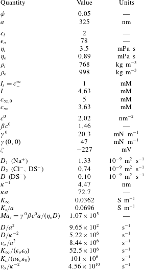
Representative set of model parameters ( $T=25\,^{\circ }\text{C}$) and characteristic frequencies, e.g. for the spectra plotted in figures 5 and 7. The variables that can be varied experimentally are the oil volume fraction
 $\unicode[STIX]{x1D719}$, drop size
 $a$, total surfactant concentration
 $c_{\infty ,0}$ and added salt concentration
 $c_{-}^{\infty }$. All other quantities are derived from these and known material properties, as detailed in the main text. Here
 $I_{s}$ is the ionic strength for the added salt (NaCl) with
 $I$ the total ionic strength (SDS and NaCl).

We must now address momentum conservation for the interfacial control volume. Here we note that the viscous diffusion time for the diffuse layer  $\unicode[STIX]{x1D705}^{-2}/\unicode[STIX]{x1D708}\lesssim O(10^{-17}/10^{-6})=O(10^{-11})~\text{s}$ (this is the shortest relaxation time, table 1), justifying quasi-steady hydrodynamics within the diffuse layer at frequencies
 $f\lesssim 100~\text{MHz}$. Accordingly, the fluid velocity outside the diffuse layer slips relative to the interface by the well-known Smoluchowski-slip velocity (Russel et al. Reference Russel, Saville and Showalter1989; Hunter Reference Hunter2001):
 $$\begin{eqnarray}\boldsymbol{u}_{S}=M_{S}\unicode[STIX]{x1D735}\unicode[STIX]{x1D713}^{\prime }\boldsymbol{\cdot }\boldsymbol{e}_{\unicode[STIX]{x1D703}}\boldsymbol{e}_{\unicode[STIX]{x1D703}},\end{eqnarray}$$
where the interfacial-slip mobility  $M_{S}=\unicode[STIX]{x1D701}\unicode[STIX]{x1D716}_{o}\unicode[STIX]{x1D716}_{0}/\unicode[STIX]{x1D702}_{o}$, with
 $\unicode[STIX]{x1D701}=\unicode[STIX]{x1D713}^{0}(r=a)$ the equilibrium electrostatic potential at the interface (
 $\unicode[STIX]{x1D702}_{o}$ is the aqueous-phase shear viscosity).
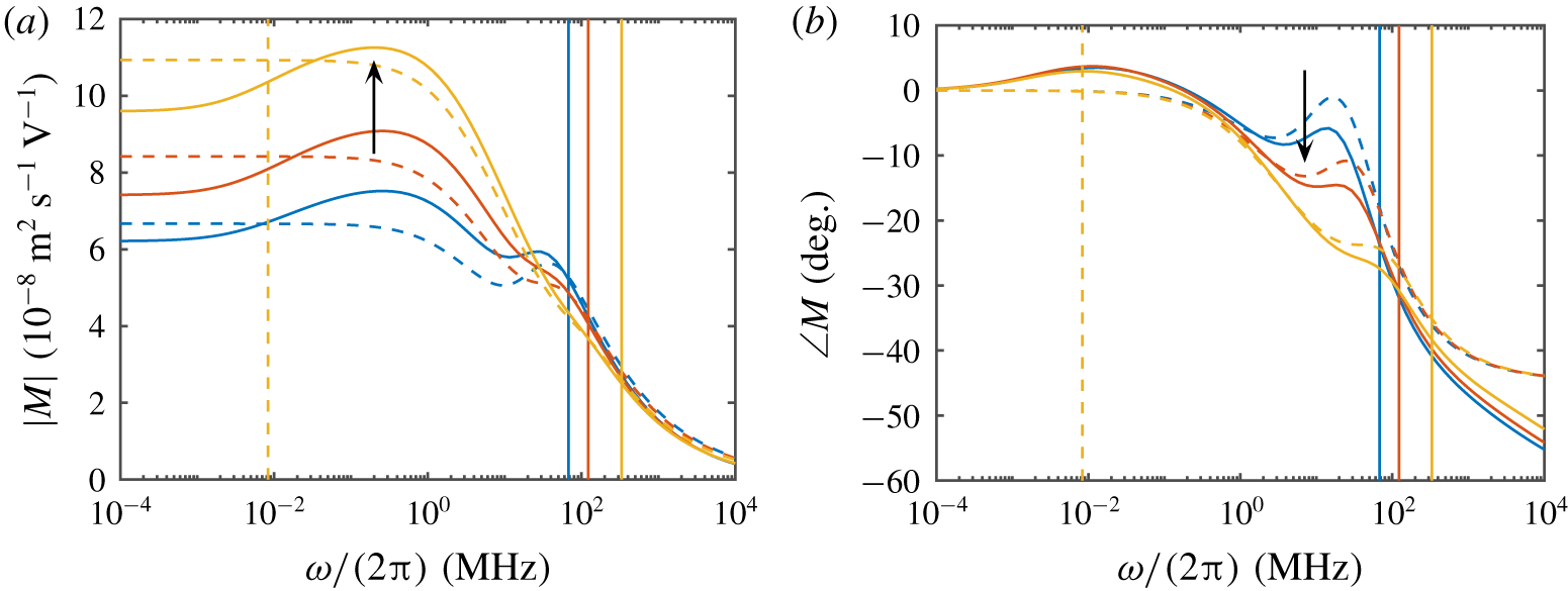
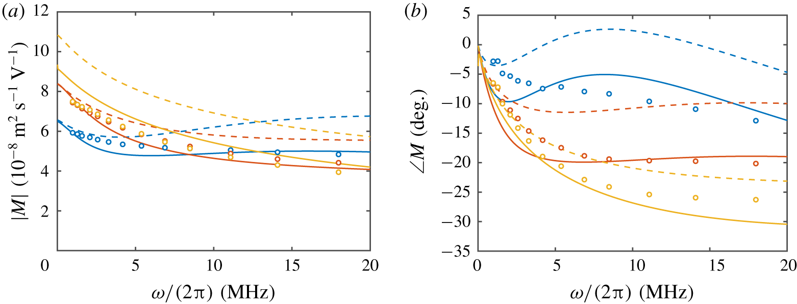
As highlighted by Hunter (Reference Hunter2001), the Smoluchowski-slip velocity emerges from a neglect (in the momentum balance) of ion-concentration perturbations in the diffuse layer. He shows that this may be questionable for highly charged interfaces, but the question still remains as to the magnitude of such errors. To assess these, we compare in figure 2 O’Brien’s dynamic mobility formula ((3.2) below, requiring  $\unicode[STIX]{x1D714}a^{2}/D\gtrsim 1$,
 $\unicode[STIX]{x1D701}e/k_{B}T\gtrsim 1$,
 $\unicode[STIX]{x1D705}a\gg 1$) with the standard electrokinetic model (Mangelsdorf & White Reference Mangelsdorf and White1992), as computed by the MPEK software package (Hill, Saville & Russel Reference Hill, Saville and Russel2003). Note that the surface potentials (
 $|\unicode[STIX]{x1D701}|\gg k_{B}T/e$) and ionic strengths are representative of the values adopted below for SDS-stabilized oil-in-water emulsions. As cautioned by Hunter (Reference Hunter2001), for these extremely highly charged interfaces, O’Brien’s formula – and therefore the theory for fluid spheres advanced here – departs somewhat from the numerically exact solutions in the megahertz range. Also consistent with Hunter’s analysis is the error diminishing with increasing
 $\unicode[STIX]{x1D705}a$.
Dynamic electrophoretic mobility spectra (magnitude and phase) for large, highly charged rigid spheres. Calculations are according to the standard electrokinetic model (solid lines) and O’Brien’s dynamic mobility formula ((3.2) with  $D=0$; dashed lines):
 $\unicode[STIX]{x1D701}=-224~\text{mV}$,
 $I=4.63~\text{mM}$ (
 $\unicode[STIX]{x1D705}a=90$, blue);
 $\unicode[STIX]{x1D701}=-215~\text{mV}$,
 $I=8.50~\text{mM}$ (
 $\unicode[STIX]{x1D705}a=120$, red); and
 $\unicode[STIX]{x1D701}=-200~\text{mV}$,
 $I=23.0~\text{mM}$ (
 $\unicode[STIX]{x1D705}a=200$, yellow). Other parameters:
 $a=400~\text{nm}$,
 $\unicode[STIX]{x1D70C}_{i}=768~\text{kg}~\text{m}^{-3}$,
 $\unicode[STIX]{x1D70C}_{o}=998~\text{kg}~\text{m}^{-3}$,
 $\unicode[STIX]{x1D716}_{i}=2$,
 $\unicode[STIX]{x1D716}_{o}=78$, aqueous NaCl electrolyte at
 $T=298~\text{K}$. Vertical lines identify the relaxation frequencies
 $D\unicode[STIX]{x1D705}^{2}$ (solid) and
 $D/a^{2}$ (dashed) with
 $D=D_{\text{Na}^{+}}=1.33\times 10^{-9}~\text{m}^{2}~\text{s}^{-1}$. Errors in the megahertz range can be attributed to ion-concentration perturbations in the diffuse layers, and thus a breakdown of the Smoluchowski-slip velocity formula (Hunter Reference Hunter2001).

Note that the net electrical force acting on the interface and diffuse layer is zero, so the tangential tractions on the interfacial control volume sum to zero:
 $$\begin{eqnarray}\boldsymbol{t}_{\unicode[STIX]{x1D703}}(r=a_{-})+\boldsymbol{t}_{\unicode[STIX]{x1D703}}(r=a_{+})-\unicode[STIX]{x1D6FE}^{0}\unicode[STIX]{x1D6FD}\unicode[STIX]{x1D735}_{s}c^{\prime }=0,\end{eqnarray}$$
with tangential slip (across the diffuse layer)
 $$\begin{eqnarray}\boldsymbol{u}_{\unicode[STIX]{x1D703}}(r=a_{-})+\boldsymbol{u}_{S}=\boldsymbol{u}_{\unicode[STIX]{x1D703}}(r=a_{+}).\end{eqnarray}$$
The hydrodynamic tractions, e.g.  $\boldsymbol{t}_{\unicode[STIX]{x1D703}}(r=a_{+})=\{-p\boldsymbol{I}+\unicode[STIX]{x1D702}_{o}[\unicode[STIX]{x1D735}\boldsymbol{u}+(\unicode[STIX]{x1D735}\boldsymbol{u})^{\text{T}}]\}\boldsymbol{\cdot }\boldsymbol{e}_{r}\boldsymbol{\cdot }\boldsymbol{e}_{\unicode[STIX]{x1D703}}\boldsymbol{e}_{\unicode[STIX]{x1D703}}$, are evaluated according to the fluid velocity in the bulk outer regions, and the Marangoni traction
 $-\unicode[STIX]{x1D6FE}^{0}\unicode[STIX]{x1D6FD}\unicode[STIX]{x1D735}_{s}c^{\prime }=-\unicode[STIX]{x1D6FE}^{0}\unicode[STIX]{x1D6FD}d_{c}a^{-1}\boldsymbol{X}\boldsymbol{\cdot }\boldsymbol{e}_{\unicode[STIX]{x1D703}}\boldsymbol{e}_{\unicode[STIX]{x1D703}}$ is from the perturbation in surface tension
 $\unicode[STIX]{x1D6FE}^{\prime }$ that accompanies the perturbation in the interfacial concentration
 $c^{\prime }$. Thus, with
 $\unicode[STIX]{x1D6FE}^{0}$ the equilibrium surface tension, which will be prescribed according to an equilibrium isotherm, we define
 $$\begin{eqnarray}\unicode[STIX]{x1D6FE}^{0}\unicode[STIX]{x1D6FD}=-\left.\frac{\unicode[STIX]{x2202}\unicode[STIX]{x1D6FE}}{\unicode[STIX]{x2202}c}\right|_{c^{0}}>0\end{eqnarray}$$
via the linearization  $\unicode[STIX]{x1D6FE}=\unicode[STIX]{x1D6FE}^{0}(1-\unicode[STIX]{x1D6FD}c^{\prime })$. Note that the radial traction need not be continuous: with the assumption of a spherical interface, the pressure jump is assumed to be balanced by the Laplace pressure (equilibrium value
 $2\unicode[STIX]{x1D6FE}/a$). Pozrikidis (Reference Pozrikidis1998) has shown that the pressure jump across the interface of an uncharged oscillating spherical drop is independent of position, in which case the motion does not induce a shape change. (Under steady translation, Taylor & Acrivos (Reference Taylor and Acrivos1964) showed that such drops transform to oblate spheroids and then spherical caps with increasing Weber number.) More generally, we have
 $$\begin{eqnarray}\unicode[STIX]{x0394}p=[\hat{p}(a_{-})-\hat{p}(a_{+})]\boldsymbol{X}\boldsymbol{\cdot }\boldsymbol{e}_{r}=\left[-\frac{2}{3}\sqrt[4]{-1}\sqrt{\unicode[STIX]{x1D6FA}_{i}}c_{1}^{\prime }a-\text{i}\unicode[STIX]{x1D6FA}_{o}a\left(\frac{U}{X}-c_{3}a^{-3}\right)\right]\boldsymbol{X}\boldsymbol{\cdot }\boldsymbol{e}_{r}.\end{eqnarray}$$
Finally, combining the foregoing momentum boundary conditions with the other independent conservation relationships, we must solve the following linear system for $\hat{d}_{\unicode[STIX]{x1D713}}$,
 $d_{c}$,
 $c_{1}^{\prime }$ and
 $c_{1}$ (or
 $c_{3}$):
 $$\begin{eqnarray}(\text{i}\unicode[STIX]{x1D714}a^{2}/2-D)d_{c}+a(E/X-\hat{d}_{\unicode[STIX]{x1D713}}a^{-3})zec^{0}\frac{D}{k_{B}T}+af_{r}(r=a_{-})c^{0}=0,\end{eqnarray}$$
 $$\begin{eqnarray}\displaystyle & & \displaystyle -\text{i}\unicode[STIX]{x1D714}\unicode[STIX]{x1D716}_{o}\unicode[STIX]{x1D716}_{0}(E/X+2\hat{d}_{\unicode[STIX]{x1D713}}a^{-3})+\text{i}\unicode[STIX]{x1D714}\unicode[STIX]{x1D716}_{i}\unicode[STIX]{x1D716}_{0}(E/X-\hat{d}_{\unicode[STIX]{x1D713}}a^{-3})\nonumber\\ \displaystyle & & \displaystyle \quad =2K_{s}a^{-1}(E/X-\hat{d}_{\unicode[STIX]{x1D713}}a^{-3})-K_{\infty }(E/X+2\hat{d}_{\unicode[STIX]{x1D713}}a^{-3})\nonumber\\ \displaystyle & & \displaystyle \qquad -\,2a^{-2}Dzed_{c}+2a^{-1}(E/X-\hat{d}_{\unicode[STIX]{x1D713}}a^{-3})(ze)^{2}c^{0}\frac{D}{k_{B}T},\end{eqnarray}$$
 $$\begin{eqnarray}\displaystyle & \displaystyle \unicode[STIX]{x1D702}_{o}f_{rr}(r=a_{+})=\unicode[STIX]{x1D702}_{i}f_{rr}(r=a_{-})+\unicode[STIX]{x1D6FE}^{0}\unicode[STIX]{x1D6FD}d_{c}a^{-1}, & \displaystyle\end{eqnarray}$$
 $$\begin{eqnarray}\displaystyle & \displaystyle f_{r}(r=a_{-})-M_{S}(E/X-\hat{d}_{\unicode[STIX]{x1D713}}a^{-3})=f_{r}(r=a_{+}), & \displaystyle\end{eqnarray}$$
where  $a_{+}\sim a+\unicode[STIX]{x1D705}^{-1}$ and
 $a_{-}\sim a-\unicode[STIX]{x1D6FF}$ (see figure 1). Equations (2.18)–(2.21) may be termed, respectively, interfacial adsorbed surfactant conservation, interfacial charge conservation, interfacial tangential momentum conservation, and diffuse-layer tangential slip relationships. Recall that
 $f$ and its radial derivatives are readily obtained from (2.3) and (2.4). Note that the surface conductivity
 $K_{s}$ emerging from O’Brien’s matching of current between the diffuse layer and bulk electrolyte depends on the electrolyte composition and interfacial charge density and, therefore, surface potential
 $\unicode[STIX]{x1D701}$ (O’Brien Reference O’Brien1986, Reference O’Brien1988). In this paper,
 $\unicode[STIX]{x1D701}$,
 $\unicode[STIX]{x1D6FD}$,
 $c^{0}$ and
 $\unicode[STIX]{x1D6FE}^{0}$ are furnished by a surface adsorption isotherm (detailed below) that links these variables to the composition of the bulk surfactant-containing electrolyte.
2.3 Model solution and mobility
The equations above become too cumbersome to solve in closed form, and so we evaluate the solution numerically as a linear system
 $$\begin{eqnarray}\boldsymbol{f}(\boldsymbol{x})=\mathop{\sum }_{j=1}^{4}x_{j}\boldsymbol{a}_{j}-\boldsymbol{b}=\mathbf{0}\end{eqnarray}$$
for which  $x_{j}$ are the unknowns and
 $$\begin{eqnarray}\boldsymbol{a}_{j}=\boldsymbol{f}(\boldsymbol{e}_{j})+\boldsymbol{b}\quad \text{with }\boldsymbol{b}=-\boldsymbol{f}(0),\end{eqnarray}$$
where  $\boldsymbol{e}_{j}$ is a vector for which the
 $j$th entry is
 $1$ and the others are
 $0$. It follows that
 $$\begin{eqnarray}\boldsymbol{x}=[\boldsymbol{a}_{1},\boldsymbol{a}_{2},\boldsymbol{a}_{3},\boldsymbol{a}_{4}]^{-1}\boldsymbol{\cdot }\boldsymbol{b}.\end{eqnarray}$$
To compute the electrophoretic mobility, we solve the system with  $U=1$ and
 $E=0$, and
 $E=1$ and
 $U=0$, furnishing, for example,
 $c_{3}^{U}$ and
 $c_{3}^{E}$, respectively. Then, since the particle equation of motion is (Mangelsdorf & White Reference Mangelsdorf and White1992)
 $$\begin{eqnarray}-\text{i}\unicode[STIX]{x1D714}\frac{4\unicode[STIX]{x03C0}a^{3}}{3}(\unicode[STIX]{x1D70C}_{i}-\unicode[STIX]{x1D70C}_{o})\boldsymbol{V}=4\unicode[STIX]{x03C0}\text{i}\unicode[STIX]{x1D714}\unicode[STIX]{x1D70C}_{o}(c_{3}^{U}\boldsymbol{V}+c_{3}^{E}\boldsymbol{E}),\end{eqnarray}$$
where the particle velocity  $\boldsymbol{V}=-\boldsymbol{U}$, the dynamic mobility (complex-valued
 $M=V/E$) is
 $$\begin{eqnarray}M=\frac{-3c_{3}^{E}a^{-3}}{-3c_{3}^{U}a^{-3}+\unicode[STIX]{x1D70C}_{i}/\unicode[STIX]{x1D70C}_{o}-1}.\end{eqnarray}$$
This linear superposition can be used to construct, for example, the flow and dipole strengths under electrophoresis:
 $$\begin{eqnarray}\boldsymbol{u}=\boldsymbol{u}^{E}-M\boldsymbol{u}^{U}\quad \text{and}\quad \hat{d}_{\unicode[STIX]{x1D713}}=\hat{d}_{\unicode[STIX]{x1D713}}^{E}-M\hat{d}_{\unicode[STIX]{x1D713}}^{U},\end{eqnarray}$$
and so on.
2.4 Surface tension and adsorption isotherm
The surface tension and its dependence on the electrolyte composition are extremely important contributions to the foregoing electrokinetic model. In addition to prescribing the Marangoni stress, the isotherm prescribes the surface-charge density and  $\unicode[STIX]{x1D701}$-potential.
Here we consider the equilibrium existing between a flat interface between oil and water containing bulk concentrations of an anionic surfactant  $c_{\infty }$ (valence
 $z=\pm 1$) and added ‘
 $1$-
 $1$’ salt with bulk concentration
 $c_{-}^{\infty }$ (anion concentration). It is assumed that only the surfactant anion adsorbs to the interface, at an equilibrium concentration
 $c^{0}=\hat{\unicode[STIX]{x1D6E4}}$. The system is exemplified by an aqueous electrolyte of sodium dodecylsulfate (SDS, anion DS
 $^{-}$ and cation Na
 $^{+}$) and sodium chloride (Na
 $^{+}$, Cl
 $^{-}$), at surfactant concentrations below the c.m.c. We must also assume here that an ionic surfactant is strongly dissociated, existing in solution as unimers (e.g. DS
 $^{-}$). With adsorption to the interface is the formation of a diffuse layer of ions. The concentrations in excess of or below the bulk values contribute to the surface excesses of each species, and it is these that all contribute to how the surface tension/free energy of the interface varies with the bulk composition.
For this system, it can be shown that the equilibrium surface tension may be evaluated from the Gibbs thermodynamic relationship (Eriksson & Ljunggren Reference Eriksson and Ljunggren1989) as
 $$\begin{eqnarray}\displaystyle \unicode[STIX]{x1D6FE}(c_{\infty },c_{-}^{\infty }) & = & \displaystyle \unicode[STIX]{x1D6FE}(0,0)-k_{B}T\int _{0}^{c_{\infty }}\frac{\hat{\unicode[STIX]{x1D6E4}}}{c_{\infty }}\,\text{d}c_{\infty }\nonumber\\ \displaystyle & & \displaystyle -\,4k_{B}T\int _{0}^{c_{\infty }}\{\cosh [\unicode[STIX]{x1D701}e/(2k_{B}T)]-1\}\sqrt{\frac{k_{B}T\unicode[STIX]{x1D716}_{o}\unicode[STIX]{x1D716}_{0}}{2(c_{\infty }+c_{-}^{\infty })e^{2}}}\,\text{d}c_{\infty },\end{eqnarray}$$
where  $\unicode[STIX]{x1D6FE}(0,0)$ is the surface tension of the oil–water interface with no surfactant or added salt. We use (2.23) to numerically evaluate the partial derivative
 $\unicode[STIX]{x1D6FD}$ for the Marangoni stress in the electrokinetic model: first,
 $c^{0}=\hat{\unicode[STIX]{x1D6E4}}(c_{\infty },c_{-}^{\infty })$ and the equilibrium surface tension
 $\unicode[STIX]{x1D6FE}^{0}=\unicode[STIX]{x1D6FE}(c_{\infty },c_{-}^{\infty })$ are computed for two bulk surfactant concentrations that are very close to
 $c_{\infty }$, and then
 $\unicode[STIX]{x2202}\unicode[STIX]{x1D6FE}^{0}/\unicode[STIX]{x2202}c^{0}$ is approximated using a centred finite-difference formula. This prescription implicitly assumes that the dynamic (non-equilibrium) perturbations in the interfacial surface tension arise solely from (lateral transport-induced) perturbations in the adsorbed surfactant concentration.
The first integral in (2.23) captures the free energy of the adsorbed layer (electrostatic, entropic and enthalpic contributions), and the second is the contribution from the diffuse layer (electrostatic and translational entropic free energies) with adsorption isotherm (Prosser & Franses Reference Prosser and Franses2001)
 $$\begin{eqnarray}\hat{\unicode[STIX]{x1D6E4}}=\frac{c_{\infty }\unicode[STIX]{x1D6E4}}{\text{e}^{ze\unicode[STIX]{x1D701}/k_{B}T}n+c_{\infty }},\end{eqnarray}$$
where the surface-charge density (Gouy–Chapman formula (Russel et al. Reference Russel, Saville and Showalter1989))
 $$\begin{eqnarray}\hat{\unicode[STIX]{x1D6E4}}ze=2\sqrt{2k_{B}T\unicode[STIX]{x1D716}_{o}\unicode[STIX]{x1D716}_{0}(c_{-}^{\infty }+c_{\infty })}\sinh [|z|e\unicode[STIX]{x1D701}/(2k_{B}T)]\end{eqnarray}$$
and (model parameters)
 $$\begin{eqnarray}\unicode[STIX]{x1D6E4}=1/(\unicode[STIX]{x03C0}a_{s}^{2})\quad \text{and}\quad n=\text{e}^{\unicode[STIX]{x0394}\unicode[STIX]{x1D716}}/(\unicode[STIX]{x03C0}a_{s}^{2}\unicode[STIX]{x1D6FF}).\end{eqnarray}$$
The integrals are evaluated numerically using iteration at each integrand evaluation to ascertain how the integrand changes with respect to the integration variable  $c_{\infty }$. In deriving the isotherm,
 $a_{s}$ is interpreted as the ‘excluded-volume’ radius of an adsorbed surfactant molecule, and
 $\unicode[STIX]{x1D6FF}$ is a length that characterizes the thickness of the interface, ultimately prescribing the translational free energy. Moreover,
 $\unicode[STIX]{x0394}\unicode[STIX]{x1D716}$ is the change in enthalpic free energy (scaled with
 $k_{B}T$) when transferring a DS
 $^{-}$ ion from the bulk solvent/water to the interface.
The calculations undertaken in this paper have, as prescribed parameters (fitted to experimental data to be published elsewhere),  $\unicode[STIX]{x1D6FE}(0,0)=0.047~\text{N}~\text{m}^{-1}$,
 $\unicode[STIX]{x0394}\unicode[STIX]{x1D716}\approx -19$ (value for similarly sized hydrocarbons transferred between water and oil) and
 $a_{s}=2.42$ Å (solution radius of an SO
 $_{4}^{2-}$ ion to represent the DS
 $^{-}$ polar head group in water). Then, setting
 $n=\text{e}^{\unicode[STIX]{x0394}\unicode[STIX]{x1D716}}/(\unicode[STIX]{x03C0}a_{s}^{2}\unicode[STIX]{x1D6FF})\approx 9.29\times 10^{-4}~\text{mmol}~\text{l}^{-1}$ as a single adjustable parameter, we find
 $\unicode[STIX]{x1D6FF}\approx 0.225a_{s}\approx 0.54$ Å, which, as expected, is small, suggesting a compact interface with weak fluctuations in the protrusion of DS
 $^{-}$ head groups from the oil–water interface.
This physically motivated approach to prescribing the model parameters provides an excellent fit to data for salt concentrations  ${\lesssim}20~\text{mmol}~\text{l}^{-1}$ and SDS concentrations below the c.m.c. (varying with salt concentration) at which point the surface tension becomes constant with further addition of surfactant, departing from the theory, which predicts a continuous decline (unphysical negative surface tension). Surface tension above the c.m.c. is
 ${\sim}0.2\unicode[STIX]{x1D6FE}(0,0)$ (Prosser & Franses Reference Prosser and Franses2001), which can be used as a guide with which to bound the isotherm to concentrations below the c.m.c.
Note that numerically integrating (2.24) yields the surface tension as furnished by formulae of Borwankar & Wasan (Reference Borwankar and Wasan1988) (which require an iterative solution) to ascertain, for example, the  $\unicode[STIX]{x1D701}$-potential. A numerical integration enables the model to be modified, e.g. to model electrostatic excluded-volume effects. Nevertheless, for the results presented in this paper, the model is applied in its most basic form to compute the equilibrium surface-charge density
 $zec^{0}$, equilibrium surface tension
 $\unicode[STIX]{x1D6FE}^{0}$, surface-tension gradient (with respect to surface concentration)
 $\unicode[STIX]{x1D6FD}$ and equilibrium
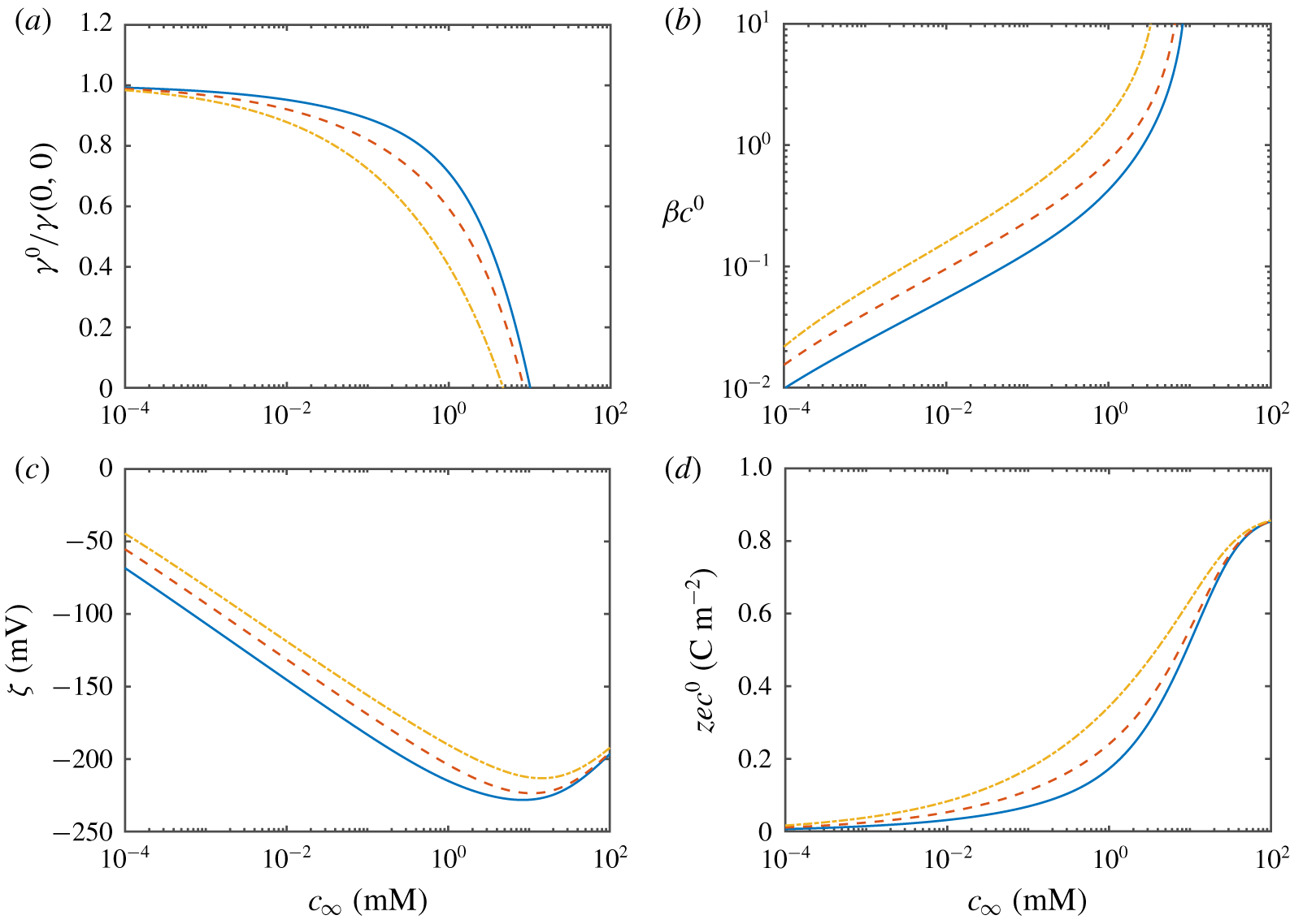
 $\unicode[STIX]{x1D701}$-potential, as required for the electrokinetic model. These are plotted in figure 3 versus the bulk SDS concentration for three representative concentrations of added salt. Note that calculations at SDS concentrations above those for which
 $\unicode[STIX]{x1D6FE}^{0}\lesssim 0.2\unicode[STIX]{x1D6FE}(0,0)$ are unphysical extrapolations of the model, since it does not account for micelle formation. We also note that the volume fraction of Na
 $^{+}$ ions at the interface can reach values of the order of close packing at high SDS concentrations and higher added salt concentrations. It may therefore be prudent to examine the role of ion-steric effects on the adsorption isotherm, e.g. as undertaken by Khair & Squires (Reference Khair and Squires2009) for interfaces with prescribed surface-charge density using the Bikerman mean-field model.
Equilibrium characteristics of the SDS–hexadecane–water interface versus the bulk SDS concentration: added salt concentrations  $c_{-}^{\infty }=1$ mM (solid),
 $5$ mM (dashed) and
 $20$ mM (dash-dotted). Note that the model is extrapolated beyond its range of validity at each ionic strength, i.e. beyond the c.m.c. to values of
 $c_{\infty }$ for which
 $\unicode[STIX]{x1D6FE}^{0}/\unicode[STIX]{x1D6FE}(0,0)\lesssim 0.2$.

Before proceeding to the results, note that sonication of oil and water with a strongly adsorbing surfactant produces an extremely large surface area, so the concentration of surfactant in the aqueous phase can be significantly lower than initially prepared. Here, we invoke the isotherm equation (2.24) with a material balance on the oil and surfactant phases to link the overall surfactant concentration  $c_{\infty ,0}$ to the actual/equilibrium bulk concentration
 $c_{\infty }$, assuming equilibrium and a monodisperse emulsion with drop radius
 $a$. In the absence of a direct measurement,
 $a$ becomes the single unknown when comparing theoretical predictions of the dynamic mobility with experiments. In practice, dynamic light scattering or acoustic attenuation may be used to independently ascertain
 $a$ and estimate its distribution.
Mass balances on the oil and surfactant (comparing the as-prepared and equilibrium states) furnish
 $$\begin{eqnarray}3\unicode[STIX]{x1D719}\hat{\unicode[STIX]{x1D6E4}}/a+c_{\infty }(1-\unicode[STIX]{x1D719})=c_{\infty ,0},\end{eqnarray}$$
where we recall that  $\unicode[STIX]{x1D719}$ is the oil volume fraction. Owing to the nonlinear manner in which the equilibrium surface concentration
 $c^{0}=\hat{\unicode[STIX]{x1D6E4}}$ depends on
 $c_{\infty }$ (using (2.24)), this is solved numerically for
 $c_{\infty }$ using a standard iterative algorithm that also furnishes
 $\unicode[STIX]{x1D6FE}^{0}=\unicode[STIX]{x1D6FE}^{0}(c_{\infty },c_{-}^{\infty })$,
 $\unicode[STIX]{x1D6FD}$,
 $c^{0}=\hat{\unicode[STIX]{x1D6E4}}(c_{\infty },c_{-}^{\infty })$ and
 $\unicode[STIX]{x1D701}$. As exemplified by pioneering electrokinetic interpretations of the ESA for dispersions of solid particulates (O’Brien Reference O’Brien1990), such a measurement furnishes mobility magnitude and phase spectra, so, at least in principle, such a measurement may furnish the particle size (O’Brien et al. Reference O’Brien, Cannon and Rowlands1995).
3 Results
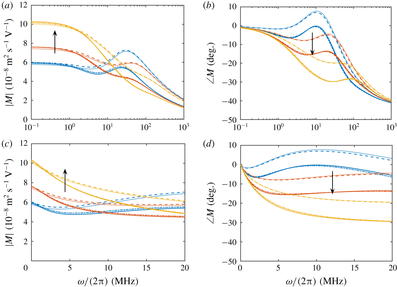
As a prelude to the dynamic mobility, § 3.1 examines the electrokinetic model from the perspective of the drag-force spectrum: for drops in the absence of an electric field. This simpler problem highlights the role of Marangoni effects, permitting comparisons with literature calculations of the dynamic drag force for spherical drops without interfacial comtaminants. Dynamic mobility spectra are presented in § 3.2, again highlighting the role of Marangoni effects.
3.1 Drag coefficient
First, for a drop that is stationary in a translating fluid (with  $\boldsymbol{E}=0$), the force exerted on the drop can be written as
 $$\begin{eqnarray}\displaystyle \boldsymbol{F} & = & \displaystyle 6\unicode[STIX]{x03C0}\unicode[STIX]{x1D702}_{o}a\boldsymbol{U}\nonumber\\ \displaystyle & & \displaystyle \times \,\left[-\frac{\text{i}\unicode[STIX]{x1D6FA}_{o}a^{2}}{3}-\frac{\displaystyle ((\text{i}-1)\sqrt{\unicode[STIX]{x1D6FA}_{o}/2}a-1)\left(2+\frac{\unicode[STIX]{x1D702}_{i}}{\unicode[STIX]{x1D702}_{o}}\frac{T_{i}(\unicode[STIX]{x1D6FA}_{i}a^{2})}{V_{i}(\unicode[STIX]{x1D6FA}_{i}a^{2})}-\frac{Ma_{c}}{\text{i}\unicode[STIX]{x1D6FA}_{o}a^{2}\unicode[STIX]{x1D708}_{o}/(2D)-1}\right)}{\displaystyle 3-(\text{i}-1)\sqrt{\unicode[STIX]{x1D6FA}_{o}/2}a+\frac{\unicode[STIX]{x1D702}_{i}}{\unicode[STIX]{x1D702}_{o}}\frac{T_{i}(\unicode[STIX]{x1D6FA}_{i}a^{2})}{V_{i}(\unicode[STIX]{x1D6FA}_{i}a^{2})}-\frac{Ma_{c}}{\text{i}\unicode[STIX]{x1D6FA}_{o}a^{2}\unicode[STIX]{x1D708}_{o}/(2D)-1}}\right],\nonumber\\ \displaystyle & & \displaystyle\end{eqnarray}$$
where the concentration Marangoni number
 $$\begin{eqnarray}Ma_{c}=\frac{\unicode[STIX]{x1D6FE}^{0}\unicode[STIX]{x1D6FD}c^{0}a}{\unicode[STIX]{x1D702}_{o}D}=\frac{\unicode[STIX]{x1D6FE}^{0}\unicode[STIX]{x1D6FD}c^{0}aa_{s}}{k_{B}T}\frac{\unicode[STIX]{x1D702}_{i}}{\unicode[STIX]{x1D702}_{o}}\end{eqnarray}$$
and  $\unicode[STIX]{x1D708}_{o}=\unicode[STIX]{x1D702}_{o}/\unicode[STIX]{x1D70C}_{o}$. Note that
 $T_{i}(\unicode[STIX]{x1D6FA}_{i}a^{2})/V_{i}(\unicode[STIX]{x1D6FA}_{i}a^{2})$ is readily evaluated using (2.7) and (2.8). For adsorbed surfactants, we expect
 $D\sim k_{B}T/(\unicode[STIX]{x1D702}_{i}a_{s})$, where
 $a_{s}$ is the hydrodynamic size of a surfactant molecule. The drag coefficient
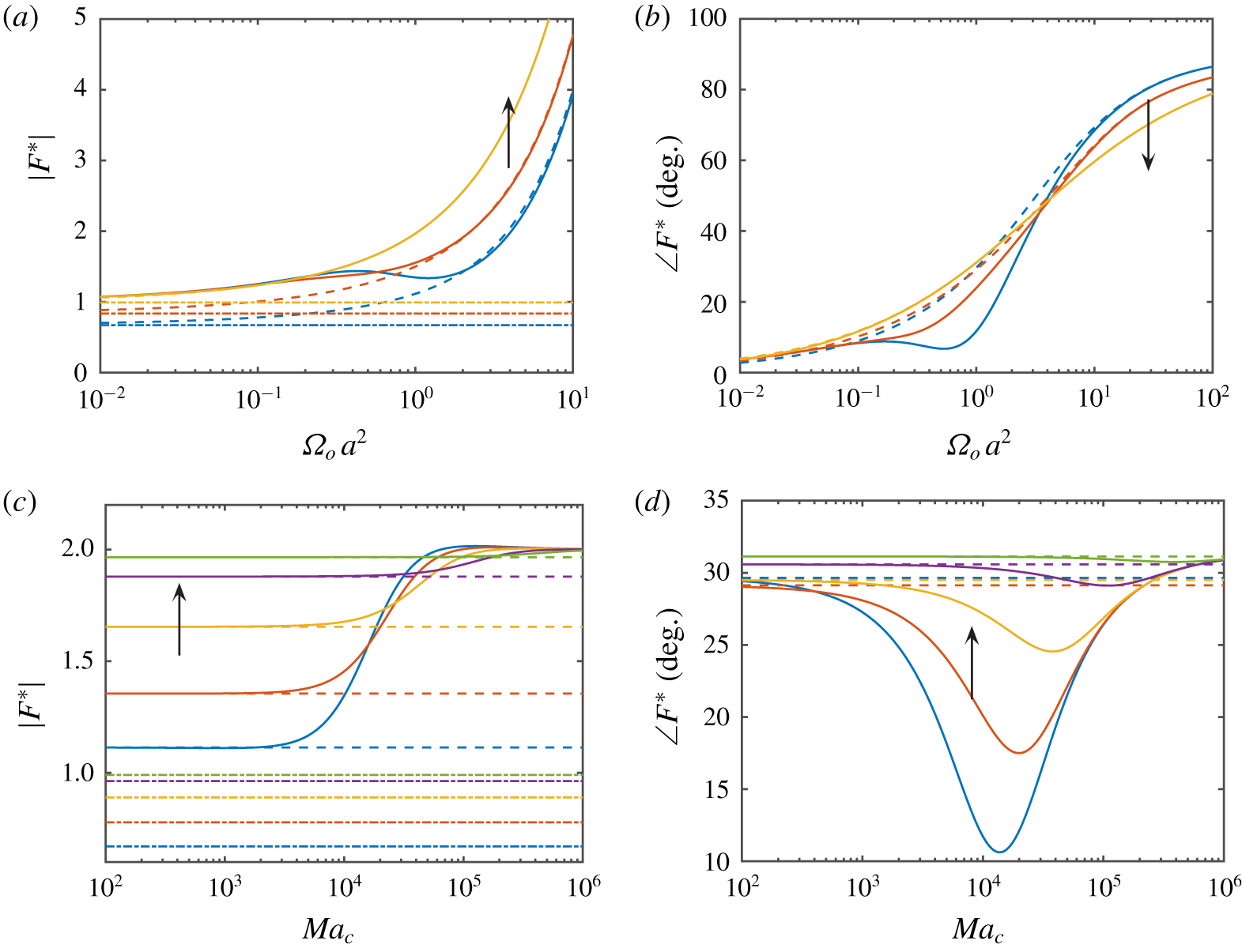
 $F^{\ast }=F/(6\unicode[STIX]{x03C0}\unicode[STIX]{x1D702}_{o}aU)$ depends on four independent dimensionless parameters, which are taken to be
 $\unicode[STIX]{x1D702}_{i}/\unicode[STIX]{x1D702}_{o}$,
 $\unicode[STIX]{x1D70C}_{i}/\unicode[STIX]{x1D70C}_{o}$,
 $\unicode[STIX]{x1D6FA}_{o}a^{2}$ and
 $\unicode[STIX]{x1D708}_{0}/D$ in the analysis of figure 4. The selected values are motivated, in part, by fluid systems for which
 $\unicode[STIX]{x1D70C}_{i}/\unicode[STIX]{x1D70C}_{o}\sim 1$,
 $\unicode[STIX]{x1D702}_{i}/\unicode[STIX]{x1D702}_{o}\sim 1$,
 $\unicode[STIX]{x1D708}_{0}/D\sim 10^{4}$ and
 $Ma_{c}\sim 10^{4}$. Moreover, at megahertz frequencies for drops with
 $a\sim 500~\text{nm}$, we have
 $\unicode[STIX]{x1D6FA}_{o}a^{2}\sim 0.1$.
Dimensionless analysis of the drag coefficient (for stationary drops in a translating fluid). (a,b) The magnitude and phase spectra for  $\unicode[STIX]{x1D702}_{i}/\unicode[STIX]{x1D702}_{o}=0.01$,
 $1$ and
 $32$ (blue to yellow),
 $\unicode[STIX]{x1D70C}_{i}/\unicode[STIX]{x1D70C}_{o}=0.8$,
 $\unicode[STIX]{x1D708}_{0}/D=10^{4}$ and
 $Ma_{c}=10^{4}$ according to (3.1) (solid lines). (c,d) The magnitude and phase for
 $\unicode[STIX]{x1D702}_{i}/\unicode[STIX]{x1D702}_{o}=0.01$,
 $0.5$,
 $2$,
 $8$ and
 $32$ (blue to green),
 $\unicode[STIX]{x1D70C}_{i}/\unicode[STIX]{x1D70C}_{o}=0.8$ and
 $\unicode[STIX]{x1D6FA}_{o}a^{2}=1$. Dashed lines: theory for drops without Marangoni stress (
 $Ma_{c}=0$), as calculated by Pozrikidis (Reference Pozrikidis1998). Dash-dotted lines: the Hadamard–Rybczynski formula (
 $Ma_{c}=\unicode[STIX]{x1D6FA}_{o}a^{2}=0$).

(a,b) Dynamic electrophoretic mobility (magnitude and phase) for spherical drops subject to a uniform electric field: drop radius  $a=325~\text{nm}$ and bulk added salt concentrations
 $c_{-}^{\infty }=1$ mM (blue),
 $5$ mM (red) and
 $20$ mM (yellow). Solid lines: full theory (numerical evaluation) for fluid spheres, including Marangoni stresses and mobile surface charge. Dash-dotted lines: closed-form approximation of the full theory for the surface-advection-dominated limit (3.3). Dashed lines: O’Brien’s formula for rigid spheres bearing immobile surface charge (e.g. (3.2) with
 $D=0$). Dotted lines: modified O’Brien theory for rigid spheres bearing mobile surface charge ((3.2) with
 $D>0$). (c,d) The same data, but over the frequency range of a commercial ESA measurement, with a linear frequency axis. Note that, with
 $c_{-}^{\infty }=20~\text{mM}$, the adsorption isotherm has been extrapolated beyond the c.m.c. and, therefore, overestimates the surface-charge density and Marangoni gradient parameter
 $\unicode[STIX]{x1D6FD}c^{0}$.

Figure 4(a,b) shows how the magnitude and phase of the drag coefficient vary with frequency for drops with three distinct viscosity ratios (same density ratio). This might be achieved experimentally by adding polymer to vary the viscosity of a low-viscosity liquid (albeit possibly imparting viscoelasticity). From a theoretical perspective, the figure highlights how the drag coefficient transits from a low-frequency rigid-sphere value (steady Stokes drag coefficient  $F=1$ as
 $\unicode[STIX]{x1D6FA}_{o}a^{2}\rightarrow 0$) to a high-frequency fluid-sphere value, as calculated by Pozrikidis (Reference Pozrikidis1998) (dash-dotted line). Note that the low-frequency limit for fluid spheres with
 $Ma_{c}=0$ is the well-known Hadamard–Rybczynski theory (horizontal lines) for which the drag coefficient varies with
 $\unicode[STIX]{x1D702}_{i}/\unicode[STIX]{x1D702}_{o}$. Figure 4(c,d) shows how the drag coefficient transits (now at a fixed frequency) from the fluid-sphere limit with
 $Ma_{c}\rightarrow 0$ to a rigid-sphere limit for which
 $Ma_{c}\rightarrow \infty$ and the drag coefficient becomes independent of the viscosity. The transition is accompanied by a distinct viscosity-contrast dependence of the phase angle. Note that the transition occurs at frequencies for which
 $\unicode[STIX]{x1D6FA}_{o}a^{2}\sim Ma_{c}D/\unicode[STIX]{x1D708}_{o}$ or
 $$\begin{eqnarray}\unicode[STIX]{x1D714}\sim \frac{\unicode[STIX]{x1D6FE}^{0}\unicode[STIX]{x1D6FD}c^{0}}{a\unicode[STIX]{x1D702}_{o}}.\end{eqnarray}$$
This is independent of  $D$, as expected based on
 $D\ll \unicode[STIX]{x1D708}_{o}$, i.e. the concentration diffusion time is very large compared to the momentum diffusion time. Under these conditions, the adsorbed surfactant advects with the interface. Thus, if we estimate the surface-advection-induced concentration gradient to be
 $O(c^{0}V\unicode[STIX]{x1D714}^{-1}/a^{2})$, then the corresponding surface-tension force is
 $O(\unicode[STIX]{x1D6FE}^{0}\unicode[STIX]{x1D6FD}c^{0}V\unicode[STIX]{x1D714}^{-1})$. Balancing this with an
 $O(V\unicode[STIX]{x1D702}_{o}a)$ viscous force furnishes the required scaling. This characteristic frequency is within the range of ESA measurements, so we should expect the transition to impact the dynamic mobility.
3.2 Dynamic electrophoretic mobility
Before examining the full dynamic mobility model, we will highlight some limiting simplifications for which closed-form expressions are readily obtained. For rigid spheres bearing mobile charge, the full model reduces to
 $$\begin{eqnarray}M=\frac{3M_{S}(1-\hat{d}_{\unicode[STIX]{x1D713}}^{E}a^{-3})((1+\text{i})\sqrt{\unicode[STIX]{x1D6FA}_{o}/2}a+\text{i})}{\frac{3}{2}\unicode[STIX]{x1D6FA}_{o}a^{2}+\frac{9}{2}((1+\text{i})\sqrt{\unicode[STIX]{x1D6FA}_{o}/2}a+\text{i})+\unicode[STIX]{x1D6FA}_{o}a^{2}(\unicode[STIX]{x1D70C}_{i}/\unicode[STIX]{x1D70C}_{o}-1)},\end{eqnarray}$$
where
 $$\begin{eqnarray}\hat{d}_{\unicode[STIX]{x1D713}}^{E}a^{-3}=\frac{\displaystyle \text{i}\unicode[STIX]{x1D714}\unicode[STIX]{x1D716}_{o}\unicode[STIX]{x1D716}_{0}-\text{i}\unicode[STIX]{x1D714}\unicode[STIX]{x1D716}_{i}\unicode[STIX]{x1D716}_{0}+2K_{s}/a-K_{\infty }+\frac{2(ze)^{2}c^{0}D\text{i}\unicode[STIX]{x1D714}a^{2}/(2D)}{ak_{B}T(\text{i}\unicode[STIX]{x1D714}a^{2}/(2D)-1)}}{\displaystyle -2\text{i}\unicode[STIX]{x1D714}\unicode[STIX]{x1D716}_{o}\unicode[STIX]{x1D716}_{0}-\text{i}\unicode[STIX]{x1D714}\unicode[STIX]{x1D716}_{i}\unicode[STIX]{x1D716}_{0}+2K_{s}/a+2K_{\infty }+\frac{2(ze)^{2}c^{0}D\text{i}\unicode[STIX]{x1D714}a^{2}/(2D)}{ak_{B}T(\text{i}\unicode[STIX]{x1D714}a^{2}/(2D)-1)}}.\end{eqnarray}$$
This is readily verified to be O’Brien’s dynamic mobility formula (O’Brien Reference O’Brien1988), but with a modified electrostatic dipole strength  $\hat{d}_{\unicode[STIX]{x1D713}}^{E}$ for the mobile surface charge. The additional terms (depending on the surface diffusion coefficient
 $D$) arise from electromigration and diffusion of the charge at the oil–water interface. Note that
 $K_{s}$ must be calculated using a formula (available in the literature) appropriate for the
 $\unicode[STIX]{x1D701}$-potential and electrolyte composition. Here, due to the very high
 $\unicode[STIX]{x1D701}$-potential furnished by the adsorption isotherm, we adopt O’Brien’s model for which the diffuse layer is occupied – to an excellent approximation – exclusively by positively charged Na
 $^{+}$ ions (O’Brien Reference O’Brien1986, equation (A.6)).
This may be compared with the phenomenological/empirical approach of Djerdjev & Beattie (Reference Djerdjev and Beattie2008), who adapted O’Brien’s dynamic mobility to fit data by adjusting  $K_{s}$ (for the diffuse layer). As highlighted in the introduction, the adjustment was comparable to the value for the diffuse layer (and was necessarily frequency-independent). The frequency-dependent correction for the adsorbed charge above is not an adjustable model parameter: it takes a value at high frequencies (
 $\unicode[STIX]{x1D714}\gg D/a^{2}$) that adds to
 $K_{s}$ an amount
 $(ze)^{2}c^{0}D/k_{B}T$. More importantly, we will see that it has a negligible impact on the dynamic mobility, because
 $D$ for DS
 $^{-}$ at the interface is much smaller than for the counterion Na
 $^{+}$ in the diffuse layer.
A more interesting simplification of the full model occurs when we neglect the surface electromigration and diffusion fluxes, assuming that the adsorbed charge advects with the interface. Recall that the surface advective flux is not divergence-free (e.g. equation (2.12)), but its contribution to the surface-charge perturbation vanishes in the model owing to the counter-advection of charge in the diffuse layer (in the linear model these are the product of an equilibrium charge density multiplied by the advective velocity perturbation). This advective organization of the interface nevertheless induces a concentration polarization that generates the Marangoni surface-tension gradient, coupling hydrodynamics to concentration polarization. In this advection-dominated surface-transport limit, the model furnishes a closed-form solution
 $$\begin{eqnarray}\displaystyle c_{3}^{X}a^{-3} & = & \displaystyle -\frac{U}{2X}\nonumber\\ \displaystyle & & \displaystyle -\,\left[\frac{\displaystyle \frac{3U}{X}+\left[\frac{\unicode[STIX]{x1D702}_{i}}{\unicode[STIX]{x1D702}_{o}}\frac{T_{i}(\unicode[STIX]{x1D6FA}_{i}a^{2})}{V_{i}(\unicode[STIX]{x1D6FA}_{i}a^{2})}-Ma_{c}\frac{2D}{\text{i}\unicode[STIX]{x1D714}a^{2}}\right]\left[\frac{3U}{2X}+M_{S}(E/X-\hat{d}_{\unicode[STIX]{x1D713}}a^{-3})\right]}{\displaystyle 3-(\text{i}-1)\sqrt{\unicode[STIX]{x1D6FA}_{o}/2}a+\frac{\unicode[STIX]{x1D702}_{i}}{\unicode[STIX]{x1D702}_{o}}\frac{T_{i}(\unicode[STIX]{x1D6FA}_{i}a^{2})}{V_{i}(\unicode[STIX]{x1D6FA}_{i}a^{2})}-Ma_{c}\frac{2D}{\text{i}\unicode[STIX]{x1D714}a^{2}}}\right]\nonumber\\ \displaystyle & & \displaystyle \times \,\frac{(\sqrt[4]{-1}\sqrt{\unicode[STIX]{x1D6FA}_{o}}a+\text{i})}{\unicode[STIX]{x1D6FA}_{o}a^{2}},\end{eqnarray}$$
with O’Brien’s electrostatic dipole strength  $\hat{d}_{\unicode[STIX]{x1D713}}$ as given by (2.16). Note that this simplification could have been anticipated by the balances of electrical and drag forces on an adsorbed surfactant molecule. Such a scaling analysis furnishes a surfactant velocity, relative to the interface velocity, that is
 ${\sim}\unicode[STIX]{x1D705}a_{s}^{2}/(\unicode[STIX]{x1D719}_{s}\unicode[STIX]{x1D6FF}_{s})$, where
 $\unicode[STIX]{x1D719}_{s}$ is the surfactant area fraction with
 $\unicode[STIX]{x1D6FF}_{s}$ a hydrodynamic size. Thus, for a crowded interface with
 $\unicode[STIX]{x1D6FF}_{s}\sim a_{s}$ and
 $\unicode[STIX]{x1D719}_{s}\sim 1$, we have
 $\unicode[STIX]{x1D705}a_{s}^{2}/(\unicode[STIX]{x1D719}_{s}\unicode[STIX]{x1D6FF})\sim \unicode[STIX]{x1D705}a_{s}\ll 1$, indicating that the surfactant dynamics are tightly coupled to the interface.
The values of  $c_{3}^{E}$ and
 $c_{3}^{U}$ from (3.3) are readily converted to a mobility using (2.22). As shown below, the mobility formula accurately mimics the full model (which requires a numerical evaluation). More importantly, it identifies distinct departures of the dynamic mobility spectrum – due to the Marangoni stresses – from those for a rigid sphere (especially in the phase, but also in the magnitude). This addresses the principal motivation for pursuing this study: whereas O’Brien’s formula captures the dynamics of a rigid sphere with immobile surface charge, equations (2.22) and (3.3) capture the internal fluid dynamics and advective migration of the charge at the interface, which induce Marangoni stresses that modulate the particle dynamics. While it is tempting to discard the terms
 $Ma_{c}2D/(\text{i}\unicode[STIX]{x1D714}a^{2})$ in (3.3) based on the requirement that
 $\unicode[STIX]{x1D714}a^{2}/D\gg 1$,
 $Ma_{c}$ may be very large, so the ratio of these terms (which captures the Marangoni effects) is non-negligible.
Interestingly, the Marangoni influences manifest in the frequency range for which ESA measurements are conducted (limited above principally by the sound wave wavelength being large compared to the particle radius). It should also be noted that (3.3) does not adjust the diffuse-layer conductivity  $K_{s}$ to account for the mobility of the adsorbed charge, i.e. as undertaken by Djerdjev & Beattie (Reference Djerdjev and Beattie2008). This clearly changes the way in which dynamic mobility might be interpreted, and may have a significant impact on the interpretation of conductivity and dielectric spectroscopy experiments.
Before discussing the results, we briefly review the model parameters, as summarized in table 1 for an SDS–hexadecane emulsion prepared with an oil volume fraction  $\unicode[STIX]{x1D719}=0.05$, overall SDS concentration
 $c_{\infty ,0}=5~\text{mmol}~\text{l}^{-1}$ and aqueous-phase NaCl concentration
 $c_{-}^{\infty }=1~\text{mmol}~\text{l}^{-1}$. Here, the overall ionic strength (aqueous SDS and NaCl)
 $I=4.63~\text{mmol}~\text{l}^{-1}$ is dominated by surfactant, furnishing a Debye length
 $\unicode[STIX]{x1D705}^{-1}=4.42~\text{nm}$ and a substantial surface potential
 $\unicode[STIX]{x1D701}=-223~\text{mV}$ that reflects a surface-charge density (DS
 $^{-}$ monolayer packing density)
 $zec^{0}=-1.9e~\text{nm}^{-2}$ (equivalent to
 $-0.3~\text{C}~\text{m}^{-2}$).
Note that applying the Smoluchowski formula for (particle) electrophoretic mobility ( $M_{S}=\unicode[STIX]{x1D716}_{o}\unicode[STIX]{x1D716}_{0}\unicode[STIX]{x1D701}/\unicode[STIX]{x1D702}_{o}$) when
 $\unicode[STIX]{x1D705}a\gg 1$ furnishes a mobility magnitude
 ${\gtrsim}17.3\times 10^{-8}\text{m}^{2}~\text{s}^{-1}~\text{V}^{-1}$, which is almost three times the mobility registered at vanishing frequency with the prevailing surface-charge density. As captured by the standard electrokinetic model, and exemplified by O’Brien’s mobility formula (e.g. equation (3.2)), this reflects the electrostatic dipole attenuating the electric field, and hence the electro-osmotic flow within the diffuse layer. Electrophoretic mobilities are often interpreted by converting measured mobility at vanishing frequency to a ‘Smoluchowski’
 $\unicode[STIX]{x1D701}$-potential. Here, such a conversion furnishes an erroneous value
 $\unicode[STIX]{x1D701}_{S}\sim -80~\text{mV}$, which is clearly much lower than the actual surface potential. Such a large discrepancy underscores the challenges (e.g. as highlighted in the introduction) that have confounded attempts in the literature to unify adsorption thermodynamics and electrokinetics. Clearly, for highly charged interfaces, it is important to apply an appropriate electrokinetic model to ensure a physically meaningful interpretation of the mobility and surface charge.
Recall that the diffuse-layer conductivity  $K_{s}$ is calculated here using a relatively simple formula that is appropriate for high surface potentials (O’Brien Reference O’Brien1986, equation (A.6)). Under these conditions, the mobility of the counterion (Na
 $^{+}$) is the only one contributing to
 $K_{s}$. For the bulk electrolyte, the three univalent ions (Na
 $^{+}$, Cl
 $^{-}$ and DS
 $^{-}$) are combined to form a binary electrolyte for which the mobility of the anion is the number-density-weighted average of those for Cl
 $^{-}$ and DS
 $^{-}$. This ensures that the bulk solution conductivity
 $K_{\infty }$ is the same as for the three-component electrolyte. The diffusion coefficient for DS
 $^{-}$ in the aqueous domain is taken to be
 $0.74\times 10^{-9}~\text{m}^{2}~\text{s}^{-1}$, according to measurements of the average molar conductivity of this ion at finite concentrations where the SDS solution conductivity increases linearly (to a good approximation) with surfactant concentration up to the c.m.c. (Benrraou et al. Reference Benrraou, Bales and Zana2003; Jalsenjak & Tezak Reference Jalsenjak and Tezak2004). Based on this value, the diffusion coefficient for DS
 $^{-}$ at the oil–water interface is prescribed to be
 $\unicode[STIX]{x1D702}_{o}/\unicode[STIX]{x1D702}_{i}\approx 0.89/3.5$ times the value in water. This assumes that the hydrodynamic size of the DS
 $^{-}$ ion is dominated by the hydrophobic tail being fully immersed in the oil phase (also neglecting steric and hydrodynamic interactions).
Dynamic mobility spectra are presented in figure 5. The blue lines correspond to the parameters and isotherm calculations summarized in table 1 (added NaCl concentration  $1~\text{mM}$), with the red and yellow lines the results of calculations undertaken with the concentration of added salt being
 $5~\text{mM}$ and
 $20~\text{mM}$. Adding salt decreases the surface potential for a given surface-charge density, thus increasing the surface-charge density
 $zec^{0}$ and decreasing the interfacial tension
 $\unicode[STIX]{x1D6FE}^{0}$. Interestingly, despite increasing the surface-charge density, the mobility magnitude decreases with increasing surface-charge density. This is counter to the expectations of the Smoluchowski formula, but is well known from the so-called mobility maximum that is the hallmark of the standard electrokinetic model (O’Brien & White Reference O’Brien and White1978), and of O’Brien’s theory for highly charged particles with
 $\unicode[STIX]{x1D705}a\gg 1$.
Figure 5 shows O’Brien’s dynamic mobility (rigid sphere, immobile surface charge, dashed lines) calculated using the  $\unicode[STIX]{x1D701}$-potential from the adsorption isotherm. This is very close to the present theory (3.2) for mobile surface charge. Next, introducing the Marangoni effects for fluid spheres, we have the full theory (solid lines) and the surface-advection-dominated limit (dash-dotted lines, via equation (3.3)). This is in very close correspondence with the full theory. The approximation (neglecting interfacial diffusion and electromigration) shows that fluid characteristics of the interface influence the dynamic mobility via the internal flow and Marangoni stress.
Scaled dynamic electrophoretic mobility (magnitude) versus viscosity ratio for  $\unicode[STIX]{x1D714}/(2\unicode[STIX]{x03C0})=1$ MHz (blue),
 $10$ MHz (red) and
 $100$ MHz (yellow). Other parameters are provided in table 1. Note that
 $D=\text{const.}$, independent of
 $\unicode[STIX]{x1D702}_{i}/\unicode[STIX]{x1D702}_{o}$. Dashed line is
 $(\unicode[STIX]{x1D702}_{i}/\unicode[STIX]{x1D702}_{o})/(\unicode[STIX]{x1D702}_{i}/\unicode[STIX]{x1D702}_{o}+2/3)$ (Booth Reference Booth1951).

Performing the same calculations but with the Marangoni parameter  $c^{0}\unicode[STIX]{x1D6FD}\approx 0$ (results not shown) produces a mobility magnitude spectrum that is the same as for a rigid sphere, but shifted down by approximately one mobility unit (i.e.
 $10^{-8}~\text{m}^{2}~\text{s}^{-1}~\text{V}^{-1}$), and with the phase-angle spectrum remaining close to those in figure 5 for fluid spheres. This suggests using the phase-angle spectrum to unambiguously identify fluid behaviour. Note also that maintaining the same Marangoni stress but decreasing the internal viscosity profoundly changes the mobility spectra, depending also on whether we adjust the surface diffusivity
 $D$ accordingly. As expected, increasing the internal viscosity transits to the rigid-sphere limit. These observations highlight the important roles of Marangoni stresses and internal fluid motion on the dynamic mobility spectra for highly charged nano-drops. They also suggest that the mobility spectra for low-viscosity liquids and bubbles may be significantly influenced by the fluid and interfacial effects addressed here.
Figure 6 shows how the dynamic mobility magnitude varies with the viscosity ratio at three frequencies in the megahertz range. At the lowest frequency, the mobility, when scaled with the rigid-sphere value, coincides with Booth’s function (highlighted in the introduction) for steady electrophoresis of drops without Marangoni effects. At higher frequencies, when the Marangoni effects are activated, the mobility is enhanced (relative to Booth’s function) by a low internal viscosity, and attenuated with a high internal viscosity. As discussed by Baygents & Saville (Reference Baygents and Saville1991a) (in the context of steady electrophoresis), the mobility reflects a subtle balance of the Maxwell, Marangoni and viscous shear forces.
Accompanying the fluctuating concentration is a fluctuating surface concentration and pressure differential. As shown in figure 7, the phase of the surface-concentration dipole varies significantly with respect to the electrolyte composition in the frequency range  $1$–
 $100~\text{MHz}$, with the magnitude of the concentration polarization (scaled with
 $c^{0}$, which varies with the electrolyte composition according to the isotherm) decreasing significantly with frequency, practically independent of the electrolyte composition. The dynamic pressure differential increases approximately linearly with the frequency. This scaling reflects the temporal inertia of the fluid dynamics. There is a weak influence that is coupled to variations in the concentration polarization, and, therefore, to the Marangoni/interfacial effects. Nevertheless, the pressure differential is evidently small compared to the equilibrium Laplace pressure, suggesting that it is reasonable to have assumed a spherical shape from the outset.

Streamlines of the flow for the  $U$-,
 $E$- and electrophoresis boundary conditions are shown in figure 8. Comparing the flows at the three frequencies, spanning two orders of magnitude, in the range for which many diagnostic measurements are undertaken, including conductivity, dielectric spectroscopy and ‘static’ electrophoretic mobility measurements, highlights the role of internal flow and of temporal inertia in shaping the streamlines at high frequencies. For the
 $U$-problem (no electric field), the velocity disturbance is that prevailing with the passage of a sound wave (wavelength
 $\gg a$) in a dilute dispersion. Differences in the streamlines (with respect to
 $\unicode[STIX]{x1D714}$) reflect the momentum diffusion length
 $\sqrt{\unicode[STIX]{x1D708}_{o}/\unicode[STIX]{x1D714}}$ being comparable to the drop radius
 $a$ at these frequencies, e.g.
 $\unicode[STIX]{x1D6FA}_{o}a^{2}\sim 1$ at
 $f\sim 8~\text{MHz}$. When subjected to an electric field, transfer of momentum to the internal fluid increases with frequency, and the coupling of the electro-osmotic flow in the diffuse layer to the outer flow produces a distinct recirculation, the extent of which is limited by the momentum diffusion length
 $\sqrt{\unicode[STIX]{x1D708}_{o}/\unicode[STIX]{x1D714}}$. This confirms the inferences in § 3.1 on the transition from a rigid to a fluid interface when
 $\unicode[STIX]{x1D6FA}_{o}a^{2}\sim Ma_{c}D/\unicode[STIX]{x1D708}_{o}$. The superposition of the
 $U$- and
 $E$-flows to solve the electrophoresis problem (right panels of figure 8) produces a weak external velocity disturbance. As is well known (O’Brien & White Reference O’Brien and White1978), this reflects the electroneutrality of the particle and its diffuse layer: the applied electric field does not exert a net force on the fluid, so the slowest-decaying disturbances in the
 $U$- and
 $E$-problems vanish upon their superposition (leaving a more rapidly decaying irrotational disturbance).
Streamlines (equally spaced isocontours of the streamfunction  $frX\sin ^{2}\unicode[STIX]{x1D703}$ in the particle frame) for the
 $U$-,
 $E$- and mobility problems (left to right) according to the full model:
 $\unicode[STIX]{x1D702}_{i}/\unicode[STIX]{x1D702}_{o}\approx 3.5/0.89$;
 $a=325~\text{nm}$;
 $\unicode[STIX]{x1D714}/(2\unicode[STIX]{x03C0})=1$,
 $10$ and
 $100~\text{MHz}$ (top to bottom), with other parameters as set out in table 1. The increasing internal recirculation with frequency highlights the transition from a rigid- to a fluid-behaving interface.

Before concluding, we briefly compare fluid- and rigid-sphere models with three dynamic mobility spectra (from a Colloidal Dynamics, LLC, AcoustoSizer II ESA instrument) for SDS-stabilized hexadecane emulsions in figure 9. Here, the total SDS concentration is fixed at  $5$ mM with three concentrations of added NaCl:
 $1$,
 $5$ and
 $20~\text{mM}$. Note that, in contrast to customary theoretical interpretations of such spectra, we have adjusted only one model parameter, the drop radius
 $a$. In general, it seems reasonable to conclude that the fluid-sphere model captures the magnitude and phase better than the rigid-sphere model. A notable breakdown of both models occurs in the mobility magnitude with
 $20~\text{mM}$ of added salt. However, at the prevailing concentrations of surfactant and salt, this experiment is conducted above the c.m.c., and under conditions where the concentration of Na
 $^{+}$ ions at the interface probably brings ion-steric effects into play. We cannot be sure why this adversely impacts the model prediction of the mobility magnitude, while furnishing a remarkably excellent prediction of the phase. It is therefore our intention to investigate this – from a much more comprehensive experimental perspective – in a future study.
Dynamic electrophoretic mobility (magnitude and phase) for hexadecane volume fraction  $\unicode[STIX]{x1D719}=0.05$, bulk SDS concentration
 $c_{\infty ,0}=5~\text{mM}$ and added NaCl concentrations
 $c_{-}^{\infty }=1$ mM (blue),
 $5$ mM (red) and
 $20$ mM (yellow). Solid lines: full theory (fluid sphere, mobile surface charge). Dashed lines: O’Brien’s formula (rigid spheres, immobile surface charge). Symbols: experimental data. Theory is evaluated with a drop radius
 $a=400~\text{nm}$. With
 $c_{-}^{\infty }=20~\text{mM}$, the SDS concentration is above the c.m.c., so the theoretical adsorption isotherm overestimates the surface-charge density and Marangoni gradient parameter
 $\unicode[STIX]{x1D6FD}c^{0}$. In this regime, the adsorption (and dynamics) may also be subject to ion-steric effects, presently not accounted for.

4 Summary
We have developed an approximate theoretical model for the dynamics of non-conductive, ionic-surfactant-stabilized nano-drops under oscillatory forcing. The model is advanced with several simplifying approximations for thin, highly charged interfaces. Most notably, we neglected ion-concentration perturbations in the diffuse and bulk regions, and the exchange of surfactant between the interface and the immediately adjacent electrolyte. The first is questionable for highly charged interfaces, but there is presently no obvious remedy, other than pursuing a direct numerical solution. The other approximations are reasonable provided that the frequency is much higher than the characteristic reciprocal surfactant exchange time and the characteristic reciprocal diffusion time. Such conditions prevail at the megahertz frequencies encountered in electroacoustic and dielectric spectroscopy.
The model integrates an equilibrium adsorption isotherm to predict how the interfacial charge and surface tension depend on the emulsion composition. An analytical solution of the species, charge and momentum conservation relationships furnishes the dynamic electrophoretic mobility spectrum. As highlighted by our dimensional analysis of the drag coefficient, the full model adds three dimensionless parameters to the standard rigid-sphere model: drop viscosity ratio, ratio of the surface-concentration and fluid-momentum diffusivities,  $D/\unicode[STIX]{x1D708}_{o}$, and concentration Marangoni number,
 $Ma_{c}$.
For SDS-stabilized hexadecane nano-drops,  $D/\unicode[STIX]{x1D708}_{o}\ll 1$ and
 $Ma_{c}\gg 1$, in which case the interface undergoes a transition from rigid to fluid state at frequencies for which
 $\unicode[STIX]{x1D714}a^{2}/\unicode[STIX]{x1D708}_{o}\sim Ma_{c}D/\unicode[STIX]{x1D708}_{o}$. Under these conditions, surfactant transport on the interface is advection-dominated. This simplifies the full model so that electrostatic polarization of the drop is dominated by dynamics of the diffuse-layer charge, and can therefore be modelled using O’Brien’s dipole formula (for immobile surface charge). Accordingly, previous attempts to fit rigid-sphere electrokinetic theory to ESA spectra by invoking an ad hoc adjustment of the diffuse-layer surface conductivity might not be appropriate.
When combined with a surface-adsorption isotherm derived from surface-tension measurements, the electrokinetic model provides a self-consistent interpretation of dynamic electrophoretic mobility. The interpretation does not require the isotherm to be modified to account for counterion condensation or partial ionization, and it does not require a dynamic Stern layer with unknown mobility and capacitance parameters.
For SDS-stabilized hexadecane drops, the model predicts experimentally measured magnitude and phase spectra, with the drop size as the only fitting parameter. The radius of the drops in our experiments is inferred to be  ${\sim}400~\text{nm}$, which is in reasonable accord with the size inferred by acoustic attenuation.
We acknowledge that much more comprehensive experimental evaluation is required. This is beyond the scope of the present theoretical focus, and will therefore be undertaken in a separate study. For example, the present model identifies regimes at higher surfactant and added-salt concentrations where micelle formation and ion-steric effects (not accounted for in the present work) may be important. These would limit the present theory to lower surfactant and added-salt concentrations (and relax constraints posed by our neglect of ion-concentration perturbations in the diffuse layer).
Nevertheless, if SDS-stabilized emulsions – even at low surfactant concentrations – turn out to have the high surface-charge densities inferred by the isotherm of Borwankar & Wasan (Reference Borwankar and Wasan1988), it will be interesting to revisit earlier interpretations of  $\unicode[STIX]{x1D701}$-potential for these interfaces by accounting for the strong electrokinetic polarization effect, as captured by the standard electrokinetic model and, in part, the thin-double-layer model of O’Brien (Reference O’Brien1988). Considerable caution should be applied when adopting the Smoluchowski formula to convert mobilities to
 $\unicode[STIX]{x1D701}$-potential for such highly charged interfaces, since this may significantly underestimate the actual charge density – even when
 $\unicode[STIX]{x1D705}a\gg 1$.
On the other hand, the conclusions drawn by Roke and her coworkers (de Aguiar et al. Reference de Aguiar, de Beer, Strader and Roke2010) – that DS $^{-}$ ions occupy an anomalously large surface area – require radical revisions to existing interfacial thermodynamic models to achieve thermodynamic and electrokinetic consistency. Interestingly, an anomalously low surface-charge density would presumably improve the validity of our neglect of ion concentration perturbations in the diffuse layer. We suspect that much more attention needs to be given to accurately measuring and reporting drop size and its distribution in nanoemulsions.
Acknowledgements
This work was supported by an NSERC Discovery Grant to R.J.H., and a PRESSID/PTDF scholarship (Nigeria) to G.A. The authors thank Dave Cannon and Richard O’Brien (Colloidal Dynamics, LLC) for suggesting this problem and providing helpful feedback. We are also grateful to three anonymous referees for their constructive advice on revising the manuscript. R.J.H. acknowledges the Fields Institute for funding to present part of this work at their workshops on ion transport (2017, 2019).
Declaration of interests
The authors report no conflict of interest.
Authors’ contributions
R.J.H. performed the theoretical calculations and wrote the manuscript. G.A. performed surface-tension and electrokinetic-sonic-amplitude experiments that were used to motivate and guide the theory. These data will be reported in detail elsewhere.