Computational performance

Before many-body potentials, there were pair or two-body potentials. Classic examples are the Lennard-Jones 6–12 potential (LJ)Reference Jones⁴ (for van der Waals interactions) and Coulombic interactions between charged particles. It is worth noting these two potentials are still commonly used for modeling non-bonded interactions in all-atom biological and polymeric simulations (e.g., for solvated proteins). In force fields, such as CHARMmReference MacKerell, Bashford, Bellott, Dunbrack, Evanseck, Field, Fischer, Gao, Guo, Ha, Joseph-McCarthy, Kuchnir, Kuczera, Lau, Mattos, Michnick, Ngo, Nguyen, Prodhom, Reiher, Roux, Schlenkrich, Smith, Stote, Straub, Watanabe, Wirkiewicz-Kuczera, Yin and Karplus⁵ and AMBER,Reference Cheatham and Young⁶ for these systems, the non-bond terms are augmented by a list of permanent bonds within each molecule’s topology, connected by harmonic springs. Additional terms represent covalent bond bending and torsion energies.

In contrast, many-body potentials, as the name implies, explicitly include many-body effects. The energy expression for the potential is typically written as a sum over interactions that involve not just two, but clusters of three or more nearby atoms. Unlike the permanent bonds in biological models, the atoms participating in each interaction depend on their current configuration, so that covalent bonds can effectively break and form again as atoms move.

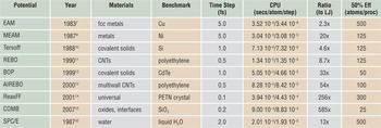
Table I lists eight such many-body potentials, the year they were first published, materials they are commonly used to model, and a typical time step size when used in a molecular dynamics simulation. The SPC/E water potential, used in biomolecular models, is included for comparison; it is computed via pairwise LJ and Coulombic interactions with additional constraints to rigidify each molecule. We next describe a few salient features of these many-body potentials that impact their computational cost. The timing information in the table is discussed later in the text.

Table I.

Many-body potentials.

Many-body potentials (except SPC/E) discussed in this article, with their publication date, typical materials they model, and time step size for molecular dynamics simulation. The two CPU times are for small (32 K atom) and large (1 M atom) simulations. The ratio is the small-problem CPU time relative to a simple Lennard-Jones potential. The 50% efficiency metric is taken from Figure 1.

EAM, embedded-atom method; MEAM, modified embedded-atom method; REBO, reactive empirical bond order; BOP, bond–order potential; AIREBO, adaptive intermolecular REBO; ReaxFF, reactive force field; COMB, charge optimized many-body; CNT, carbon nanotube.

The embedded-atom method (EAM) potentialReference Daw and Baskes^7, Reference Daw and Baskes⁸ combines a pairwise interaction with a second term representing the energy of embedding each atom in the electron density produced by its neighbors. This term elegantly captures the compressibility of the electron gas formed by valence electrons in metals, without resorting to a special volume-dependent energy term. Computing this embedding energy and its derivative (force) requires two computational loops over neighbors: one to sum electron densities so the embedding function can be evaluated for each atom, and a second to calculate the force on each atom due to its contribution to its neighbors’ embedding energies. This is the source of the effective many-body nature of the potential and a common computational motif in all the potentials discussed here (see the sidebar).

The modified EAM (MEAM) potentialReference Baskes⁹ has a similar mathematical structure to EAM, except that the electron density is given by a more complicated expression involving sums over three-body contributions that depend on the angle θ_ijk subtended by atoms j and k at a central atom i.

The Tersoff potentialReference Tersoff¹⁰ uses a short-range pair potential to represent covalent bonding. The key innovation is the concept of bond order, which plays a central role in many-body potentials such as BOP (bond-order potential) and REBO (reactive empirical bond order) and ReaxFF (reactive force field) potentials. In the Tersoff potential, the energy of a bond is modulated by the angular location of neighbor atoms relative to the bond axis.

The REBO potentialReference Brenner¹¹ extends the bond-order approach to differentiate between σ and π bonds, which increases the stability and torsional stiffness of double and triple carbon-carbon bonds. The adaptive intermolecular REBO (AIREBO) potentialReference Stuart, Tutein and Harrison¹² extends the REBO potential by adding dispersion interactions between nearby atoms leading to effective six-body interactions. The BOPReference Pettifor and Oleinik¹³ uses the tight-binding theory of bond formation to describe the energetics of covalently bonded materials.

The ReaxFF potentialReference van Duin, Dasgupta, Lorant and Goddard¹⁴ is a variable-charge bond order potential. In addition to handling conventional covalent bonding contributions, such as bond formation, stretching, bending, and torsion, it also explicitly represents a range of additional chemical bonding features, such as hydrogen bonding and bond conjugation. Charge equilibration is handled by the iterative solution of a linear system of equations representing the electronegativity equalization conditions. The need to compute long-range electrostatic interactions is eliminated by using a smoothly truncated Coulombic potential.

The charge-optimized many-body potential (COMB)Reference Yu, Sinnott and Phillpot¹⁵ is also a variable charge bond-order potential, developed to treat interfaces, oxides, and other compounds. The charges on atoms are adjusted at each time step according to the electronegativity equalization method,Reference Rick, Stuart and Berne¹⁶ which minimizes the total electrostatic energy of the system. Computation of long-range electrostatics is avoided by using the short-range Wolf summation method.Reference Wolf, Keblinski, Phillpot and Eggebrecht¹⁷

These are computational issues associated with these many-body potentials, which increase their complexity and cost:

• • As the level of many-body dependencies increases, multiple and/or nested computational loops are needed to identify neighbors, neighbors of neighbors, etc. This likewise implies longer cutoff distances as atoms are influenced by atoms further away.

• • As discussed for the EAM potential, there are intermediate stages to the computations where many-body terms are summed over interactions. In parallel, this typically requires extra communication to acquire the terms from atoms owned by different processors.

• • Identifying nearby groups of atoms that interact often requires that each atom store a “full” list of all its neighbors, rather than the typical “half” lists that suffice for enumerating pairwise interactions, due to pairwise forces being equal and opposite.

• • For potentials that include variable charge (e.g., ReaxFF and COMB), charge equilibration is effectively a long-range interaction that incurs additional cost. However, computing true long-range Coulombics (e.g., via an Ewald summationReference Ewald¹⁸) is avoided by the use of approximate methods that truncate interactions within a cutoff distance.

The potentials in Table I have all been implemented in our parallel molecular dynamics (MD) package LAMMPS,^19, Reference Plimpton²⁰ which allows us to compare their computational cost.Footnote ^† One feature of LAMMPS that makes it attractive for use in materials modeling is that it was designed to allow users to easily add functionality, such as a new potential, through well-defined interfaces. Evidence of this is that several of the potentials in Table I were implemented by individuals, including students, with only limited interaction with the LAMMPS developers.

The author of a potential writes code that computes per-atom forces and energies, as well as sets up or reads user-defined parameters (e.g., from a file). The LAMMPS infrastructure provides neighbor lists of various kinds, enables the potential to be used in hybrid simulations where two or more potentials are used to compute interactions between different groups of atoms (e.g., water or polymer chains on a metal surface), performs time integration, and computes additional analyses or diagnostics as requested by the user. Diagnostics can include per-atom virials and total energy and pressure, which can be derived from the per-atom energies and forces, eliminating the need for the potential itself to tally these quantities.Reference Thompson, Plimpton and Mattson²³

We benchmarked the relative computational cost of the LAMMPS implementation of the potentials in Table I on a Cray XT5 at Sandia National Laboratory. In each case, we ran a prototypical problem for that potential for 100 time steps, which is long enough to amortize the cost of occasional tasks such as neighbor-list building. More details on the benchmark problems are given in Reference 19, which include timing data for other pairwise and many-body potentials not discussed here.

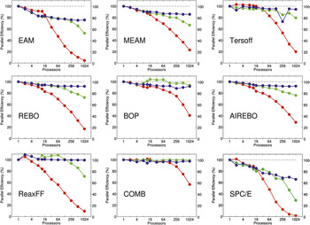
The results are shown in Figure 1. For each potential, three benchmark tests were performed. The “small” (red) and “large” (green) curves are for 32,000 (32 K) and 1,000,000 (1 M) atom systems, respectively (small variations in size for different crystal structures), run on varying numbers of processors (so-called strong-scaling results). The “scaled” (blue) curves are for systems whose size (32,000 atoms per processor) was increased in proportion to the number of processors (weak-scaling results). Thus their 1024-processor timings are for 32 M atom systems.

Figure 1.

Performance of eight many-body potentials and an SPC/E water potential on varying numbers of cores of a Cray XT5 machine, as implemented in LAMMPS.¹⁹ The red curves are for 32 K-atom systems; the green curves are for 1 M-atom systems; and the blue curves are for scaled systems with 32 K atoms per processor. Definitions of fixed-size and scaled-size parallel efficiency and the dotted line are discussed in the text. Single-core CPU times per-atom per-time step are listed in Table I. EAM, embedded-atom method; MEAM, modified embedded-atom method; REBO, reactive empirical bond-order; BOP, bond order potential; AIREBO, adaptive intermolecular REBO; ReaxFF, reactive force field; COMB, charge optimized many-body.

The plots show parallel efficiencies, where for each potential the one-processor timing is assumed to be 100% efficient (dotted lines). For the strong-scaling (red/green) curves, parallel efficiency is defined as the one-processor CPU time T ₁ divided by the P-processor time T_P, multiplied by (100/P). Thus a 1024-processor efficiency of 50% means the 32 K- or 1 M-atom problem ran 512 times faster than it did on one processor. For the weak-scaling (blue) curves, parallel efficiency is simply 100 T ₁/T_P, so that a 50% value means the 32 M-atom problem ran two times slower on 1024 processors than the 32 K-atom problem did on one processor.

Note that single-processor CPU times vary greatly between the potentials, as listed in Table I, normalized on a per-atom, per-time step basis. Also note that the typical time step size is different for different potentials. These timings are for full simulations, which include the cost of neighbor-list building and time integration. However, the vast majority of time, even for the cheapest potentials, is spent in computing the many-body interactions.

Several trends are evident from the plots in Figure 1:

• • The weak-scaling (blue) curves for all the many-body potentials show excellent scalability as the problem size and processor counts increase. This is because all of them, even the expensive ones, are essentially short-range in nature. (The nominally long-range charge-equilibration calculations for ReaxFF and COMB do not affect this, at least for these benchmark problems.) This means their computational complexity scales linearly with N/P for the number of atoms N and processors P, so long as there are sufficient atoms per processor. This is also reflected in the single-processor timings listed in Table I, which are nearly identical for the small 32 K- and large 1 M-atom problems, when normalized on a per-atom basis. The one exception is the blue curve for SPC/E. The degradation in efficiency is due to the long-range Coulombic calculation performed via the particle-particle, particle-mesh (PPPM) methodReference Hockney and Eastwood^24, Reference Pollock and Glosli²⁵ in LAMMPS, or the related particle-mesh Ewald (PME) methodReference Darden, York and Pedersen²⁶ in other MD codes. These are FFT-based methods with an O(NlogN) complexity in the number of atoms, so their cost grows as the system size increases.

• • The strong-scaling curves show reasonable scalability until the efficiency rolls off as the number of atoms per processor becomes too small. This happens more quickly for the 32 K-atom problem (red) than for the 1 M-atom problem (green) and for cheaper potentials than for more expensive ones. Again, the SPC/E potential has the worst strong-scaling behavior, due to the high communication costs of the parallel 3D FFTs needed for long-range Coulombic calculations.

• • Many of the curves show different efficiency behavior for fewer versus more than 12 processors. This is typical of the performance of many codes on multi-core nodes and reflects the architecture of the compute nodes in our Cray XT5, which contain dual hex-core processors (12 cores/node). Within a single node, running in parallel on more cores incurs memory-bandwidth bottlenecks that degrade single-node performance. In weak-scaling mode (blue), adding nodes does not degrade performance further, since the additional time spent on inter-node communication remains small relative to the computation. However, for the strong-scaling results (red), adding more nodes reduces the number of atoms per node, which can degrade efficiency more rapidly if the inter-node communication is more costly than the reduced on-node computation.

The overall message of these benchmarking data is that many-body potentials perform or scale in molecular dynamics calculations with a cost that increases linearly with the number of atoms, which means very large calculations can be performed. The data from the table and plots can be used to estimate the time to run any size system on a given number of processors, so long as there are a few hundred atoms or more per processor (less for more expensive potentials). The last column in Table I shows an estimate of the threshold for each potential, from the 32 K-atom timings, to maintain a parallel efficiency of 50% or greater.

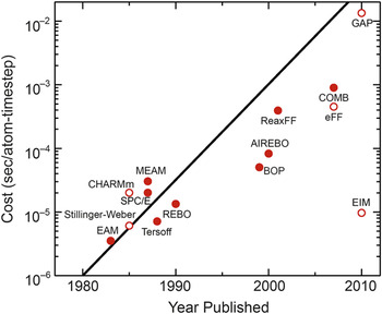
Another way to illustrate the growing computational complexity of many-body potentials over time is with the plot in Figure 2, similar to the familiar Moore’s law for the exponential growth of transistor counts in semiconductor chips. The years and timings are taken from Table I for the small-system runs on a single Cray XT5 processor. The closed symbols are for potentials discussed here; the open symbols are for other (mostly many-body) potentials available in LAMMPS.¹⁹ One exception is the new Gaussian-approximation potential or GAP, which is not yet available in the public distribution of LAMMPS.

Figure 2.

Single CPU cost in seconds per-atom per-time step versus year for the potentials of Table I (closed symbols) and others (open symbols). The line represents a doubling in computational cost every two years, akin to Moore’s Law for hardware complexity.¹⁹ EAM, embedded-atom method; MEAM, modified embedded-atom method; REBO, reactive empirical bond order; BOP, bond-order potential; AIREBO, adaptive intermolecular REBO; ReaxFF, reactive force field; COMB, charge optimized many-body; GAP, Gaussian approximation potential.

It is important to note these are timings for running all of the potentials on today’s hardware. If they were timings from the year they were developed, the slope in the data points would be closer to flat. Table I also gives a ratio of the CPU cost for the many-body potentials relative to the Lennard-Jones 6–12 pairwise potential,Reference Jones⁴ which runs at 1.54 × 10^–6 s/atom/time step in LAMMPS (for a liquid state point).Footnote ^‡

The GAP potentialReference Bártok, Payne, Kondor and Csányi²⁷ shown at the upper right of Figure 2 was developed in 2010 with the goal of providing near quantum-level accuracy in an empirical potential for systems it is appropriately fit to via comparison to a large database of quantum-calculated energies and forces, as illustrated in Figure 3 of Reference Reference Bártok, Payne, Kondor and Csányi27. It continues the trend of Figure 2, since our preliminary investigations indicate that evaluating its large set of spherical-harmonic basis functions is an order-of-magnitude more expensive than any of the many-body potentials in Table I.

Figure 3.

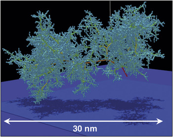
Tree structure of an 85 keV collision cascade in δ-Pu at 600 K, simulated with a modified embedded-atom method potential. The colors represent the kinetic energy of the atom; red = high, yellow = medium, green = low. Reprinted with permission from Reference Reference Kubota, Wolfer, Valone and Baskes31. ©2007, Springer Science + Business Media.

The cost of empirical potentials can also be compared to quantum density functional theory (DFT) calculations. A collaborator, Thomas Mattsson at Sandia National Laboratory, gave CPU timings for several large systems he has recently modeledReference Mattsson and Desjarlais^28, Reference Root, Magyar, Carpenter, Hanson and Mattsson²⁹ via quantum dynamics calculations with the VASP program,Reference Kresse and Hafner³⁰ using a 1 fsec time step similar to atomistic molecular dynamics. For systems with 192 and 432 atoms (1024 and 3456 electrons), the CPU times/atom/step were 252 and 1344 seconds, respectively. These single processor times were inferred from parallel runs on 384 processors, assuming 100% parallel efficiency, since they required too much memory to run on a single processor. The runs were made on a Nehalem-based Linux cluster, with single-processor performance similar to the Cray XT5 used for the atomistic simulations.

On a per-atom per-time step basis, these timings are 164 M and 873 M times, respectively, slower than the LJ timing. Thus they are five or six orders of magnitude more costly than the most expensive many-body potentials in Table I. Moreover, they indicate that unlike the empirical many-body potentials, DFT calculations do not yet scale linearly with the number of atoms (or electrons). Thus for DFT simulations of 32 K- or 1 M-atom systems, as benchmarked for the atomistic case, these ratios would be many orders of magnitude larger.

Science examples

In this section, we give brief descriptions and images from four recent large-scale simulations using the MEAM, AIREBO, and ReaxFF potentials discussed in the previous section. These were all performed on large parallel machines, using hundreds to thousands of processors and with various parallel molecular dynamics (MD) codes.

Figure 3 shows the tree-like structure of displaced atoms in a bulk plutonium (Pu) sample resulting from the recoil energy imparted to a single atom by an α-decay event as modeled in Reference Reference Kubota, Wolfer, Valone and Baskes31. Simulations with up to 16 M atoms (a 75 nm cube) were run for 2 ns to track the resulting damage and energy deposition. The MEAM potentialReference Baskes⁹ was used since it accurately models a variety of Pu phases by including angle-dependent density contributions from electrons occupying p, d, and f orbitals. These simulations were done with the pDynamo code developed by the authors,Reference Kubota, Wolfer, Valone and Baskes³¹ a parallel version of the original EAM DYNAMO code. One interesting result from the modeling was the temperature dependence of the damage persistence. At 600 K, damage slowly heals, and bulk crystal structure is recovered; at 180 K, an amorphous glass-like structure is created.

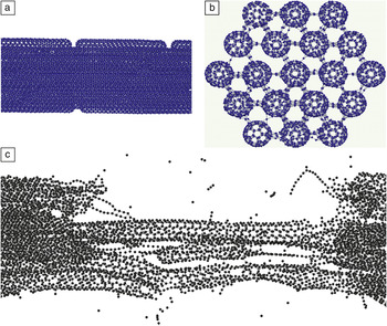
Figure 4 depicts the initial configuration of a model of fiber bundles composed of carbon nanotubes (CNTs) of varying individual length, arrayed end-to-end with cross-linking atoms and bonds added randomly between laterally adjacent CNTs, as described in Reference Reference Cornwell and Welch32. The largest systems studied were 800 nm length fibers, with 1.2 M total atoms. Strain was applied incrementally along the axis of the fiber (with relaxation time between the strain increments) over time scales up to 6 ns to measure the stress in the fiber and observe its eventual rupture, as at the bottom of Figure 4. The AIREBO potentialReference Stuart, Tutein and Harrison¹² was employed, as it has been widely used for CNT modeling and allows C‒C bonds to spontaneously form and break. These simulations were run with the LAMMPS code discussed in the previous section.¹⁹ Tensile strengths (at breakage) increased with fiber length and cross-linking density, with a value of 60 GPa observed for 800 nm fibers with cross-links involving 0.75% of the CNT atoms.Footnote ^§ This compares with a tensile strength of 110 GPa for single (5,5) CNTs used to construct the fiber.

Figure 4.

Fracture of a bundle of carbon nanotubes (800 nm in length) undergoing tensile strain, simulated with the adaptive intermolecular reactive empirical bond-order potential. (a) A side view of a portion of the unstrained fiber; (b) an end view showing cross-links between fibers; and (c) after fracture occurs, with strain applied in the lateral direction. Reprinted with permission from Reference Reference Cornwell and Welch32. ©2011, American Institute of Physics.

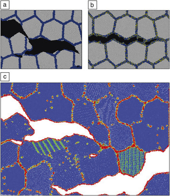
Figure 5 illustrates simulations used to elucidate atomistic mechanisms responsible for sulfur segregation‒induced embrittlement of polycrystalline nickel, presented in Reference Reference Chen, Kalia, Kaxiras, Lu, Nakano, Nomura, van Duin, Vashishta and Yuan33. The ReaxFF potentialReference van Duin, Dasgupta, Lorant and Goddard¹⁴ was used to capture the stress-induced reactions occurring between Ni and S near the grain boundaries (GBs). Models with 48 M atoms (2048 grains) were constructed for both pure Ni and Ni with 20% S in 1-nm-thick layers around the GBs. The models were large in the xy dimensions (470 nm) and thin and periodic in z (5 nm) to model a columnar grain structure. Lateral strain was applied in the vertical direction of Figure 5 to a notched sample, and fracture ensued over the course of 0.25 ns simulations performed with a parallel code developed by the authors.Reference Chen, Kalia, Kaxiras, Lu, Nakano, Nomura, van Duin, Vashishta and Yuan³³

Figure 5.

Ductile fracture of a polycrystalline sample (10 nm grains) of (a) pure Ni versus (b) brittle fracture of Ni with 20% S-doped (yellow atoms) grain boundary layers. (c) The bottom view of the pure Ni simulation is colored via the common neighborhood parameterReference Tsuzuki, Branicio and Rino³⁴ to highlight defects (non-blue) appearing at different scales. Reprinted with permission from Reference Reference Chen, Kalia, Kaxiras, Lu, Nakano, Nomura, van Duin, Vashishta and Yuan33. ©2010, American Physical Society.

The pure Ni sample (Figure 5, upper left) fractured in a ductile manner with crack-tip blunting and void formation. In contrast, the S-doped sample (upper right) fractured in a brittle manner, exhibiting only intergranular cleavage. Because atomistic simulations give the time histories of all atoms, further analysis was possible, as illustrated at the bottom of the figure. The common neighborhood parameterReference Tsuzuki, Branicio and Rino³⁴ illuminates atomic-scale defects such as dislocations as they form and move. Localized stress and energy calculations can also be performed. The authors’ analysis indicated a two-fold mechanism for S-embrittlement: a reduction in GB tensile strength, as well as a dramatic reduction in GB shear strength due to amorphization of the Ni-S phases present at the boundaries.

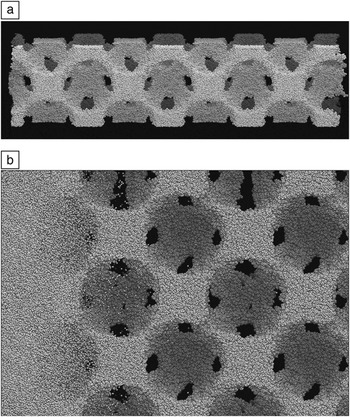
Finally, Figure 6 shows results from non-equilibrium MD simulations of the shock compression of a polymer foam constructed from several thousand 50-mer chains of poly(4-methyl-1-pentene) (PMP), as described in Reference Reference Lane, Grest, Thompson, Cochrane, Desjarlais, Mattsson, Elert, Buttler, Borg, Jordan and Vogler35. An fcc lattice of 16 nm diameter voids was introduced by growing spherical inclusions into dense samples to give an initial density of 0.3 g/cc, as at the top of the figure. The largest models were 20 x 20 x 80 nm³ in size and periodic in the lateral dimensions with 1.44 M atoms. A piston strikes the sample from the left at velocities up to 30 km/s. The simulations were performed with LAMMPS¹⁹ using the ReaxFF potentialReference van Duin, Dasgupta, Lorant and Goddard¹⁴ to allow for dissociation of the polymer bonds. A small time step of 0.025 fsec was required due to the high temperatures induced, and the shock front was tracked over a time scale of tens of picoseconds.

Figure 6.

Shock compression response of a low-density polymer foam,Reference Lane, Grest, Thompson, Cochrane, Desjarlais, Mattsson, Elert, Buttler, Borg, Jordan and Vogler³⁵ simulated using the reactive force field potential.Reference van Duin, Dasgupta, Lorant and Goddard¹⁴ (a) The initial 80-nm length foam sample and void structure. (b) A magnified view of the shock wave moving from left to right through the sample. The dark patches are locations where the voids connect to adjacent voids on the back side of the sample. Small molecular fragments are ejected into the void space ahead of the main shock front.

The bottom of Figure 6 shows the shock front, which ruptures polymer bonds and induces jetting of polymer fragments into the voids. This is in contrast to shock propagation in dense samples, which gives rise to little dissociation. The model quantitatively captures the pressure/density relationship of the material in the strong shock regime, in good agreement with experiment. The atomistic simulations also allow direct calculation of local temperature fluctuations and hot spot formation around the voids, effects that are difficult to measure experimentally.

Future issues

One software issue with using complex many-body potentials in atomistic modeling codes is that “development” is a continual process. The kernel of a Lennard-Jones potential is 10 lines of code, whereas it is thousands of lines for a potential such as ReaxFF. As bugs are found, or features added, or upgrades made by developers implementing a potential in different codes, it can be hard for users to know which version they have or which version was used in a published result. This is particularly true for many-body potentials, where their application to new materials of interest (e.g., alloys, see the Pastewka et al. article in this issue) translates to large collections of material-specific input and fitting parameters that must be carefully replicated to reproduce simulation results. The Knowledgebase of Interatomic Models (KIM) project³⁶ hopes to address these kinds of issues by providing a repository where multiple versions of many-body (and other) potentials can be time-stamped and archived, and then used by various atomistic modeling codes via a standardized interface.

On the hardware side, two trends in high-performance computing are changing the computer architectures that materials modeling codes (of all kinds, not just molecular dynamics) will commonly be running on in the future, at least at the high end.

The first is the advent of graphics processing units (GPUs) and other highly threaded many-core processors from chip makers such as NVIDIA and Intel that are increasingly attractive for scientific computing. The second is the push for exascale computing by the US Department of Energy (and other government agencies in the United States and worldwide). In this context, “exascale” means large machines, 1000x more powerful than today’s state-of-the-art petascale machines (peta = 10¹⁵ floating point operations per second). Aiming for maximum floating-point performance (flops) at low cost on a few-year timeframe is driving the design and commissioning of “hybrid” supercomputers, whose compute nodes contain both many-core CPUs and GPUs.

Extracting high performance from these machines will require a different style of programming, both for algorithm design and low-level coding. Parallelism will need to be exploited at several levels (vector operations, multi-threading, message-passing), and memory access will need to be controlled and optimized across a hierarchy of latency times and bandwidths. Computational tasks will need to be partitioned and balanced across a mixture of cores and GPUs that perform at different rates. Considerable work has already been done on these fronts to optimize molecular dynamics simulations with pairwise potentials.Reference Anderson, Lorenz and Travesset^37–Reference Stone, Phillips, Freddolino, Hardy, Trabuco and Schulten⁴⁰ But these are harder challenges for many-body potentials due to their complexity. The computational intensity of many-body potentials may translate into large speedups when they are optimized for GPUs; this is an area of active research.

We note one ancillary benefit of the trend whereby many-body potentials are becoming more expensive. On large parallel machines, a higher computational cost (per atom, relative to communication), typically means higher parallel efficiencies can be maintained with fewer atoms per core. Thus, for a simulation of a given size, the more expensive the potential, the more processors can be used efficiently. One counterbalance is that potentials with a long-range component (e.g., Coulombics) often run less efficiently with fewer atoms per processor. It is still an outstanding challenge to efficiently solve for long-range Coulombics on large numbers of processors using either FFT-based or multipole or multigrid solvers.

If the materials science community is successful in fully exploiting the capabilities of next-generation hardware for materials modeling, one outcome may be foreseen from recent successes in biomolecular modeling. New serial and parallel algorithms aimed at efficient simulation of “small” systems (e.g., tens of thousands of atoms for small solvated proteins) and the design of specialized hardware tuned for this problem, such as the Anton machine of D.E. Shaw Research, have recently enabled simulations of protein folding at the millisecond time scale (400 billion 2.5-fsec time steps!).Reference Shaw, Maragakis, Lindorff-Larsen, Piana, Dror, Eastwood, Bank, Jumper, Salmon, Shan and Wriggers⁴¹ This is allowing direct comparison with experiment, which in turn is enabling quantitative testing and improvement in the accuracy of force fields such as CHARMMReference MacKerell, Bashford, Bellott, Dunbrack, Evanseck, Field, Fischer, Gao, Guo, Ha, Joseph-McCarthy, Kuchnir, Kuczera, Lau, Mattos, Michnick, Ngo, Nguyen, Prodhom, Reiher, Roux, Schlenkrich, Smith, Stote, Straub, Watanabe, Wirkiewicz-Kuczera, Yin and Karplus⁵ and AMBER,Reference Cheatham and Young⁶ which have been used for decades in biomolecular simulations. Similar opportunities would be welcomed by developers and users of many-body potentials for materials systems.

Looking further ahead, the continued advance of computing power, coupled with innovative development of more accurate and robust many-body potentials, portends an exciting next 30 years for materials modeling. Perhaps our community can achieve the Pixar-like goal of modeling any material with quantitative atomic level accuracy via empirical potentials, at length and time scales limited only by computing resources, and all with a minimum effort by the simulator.