





1 Introduction
Understanding the fundamentals of fluid displacement processes in porous media is essential for multiple applications, from fluid uptake in diapers, humidity and fluid uptake in proton exchange membranes to carbon sequestration and enhanced oil recovery. This involves understanding the dynamics of drainage and imbibition, which however is often hard to unravel due to the complexity of the porous medium in terms of pore geometry, surface roughness and wetting properties. Attempts to simplify the problem, in order to determine the fluid displacement pathways and the associated fluid distributions, have been carried out with pore network models (Blunt et al. Reference Blunt, Jackson, Piri and Valvatne2002, Reference Blunt, Bijeljic, Dong, Gharbi, Iglauer, Mostaghimi, Paluszny and Pentland2013). Pore network models decompose the porous medium into an ensemble of geometric shapes and, based on the pioneering work of Lenormand, Zarcone & Sarr (Reference Lenormand, Zarcone and Sarr1983), predict the fluid displacement at the field scale in a sequential manner. These models have been successful especially for the drainage case, but do not work so well for the imbibition case. Our aim in this paper is to demonstrate the importance of the pore geometry in determining the displacement pathways, especially for spontaneous imbibition, by studying the displacement dynamics in well-defined single capillaries and pore junctions.
A significant amount of work has been carried out on the subject of imbibition or capillary filling. A fluid penetrates a hydrophilic capillary due to the Laplace pressure across the fluid–fluid interface, or equivalently due to the decrease in the free energy of the system as the hydrophilic liquid wets the walls of the capillary. The system uses the energy liberated from wetting the walls to drive the fluid inside the capillary. Lucas (Reference Lucas1918) and Washburn (Reference Washburn1921) gave the first account of this phenomenon, but considered only the regime when all influences apart from the driving force and the viscous drag cease to exist. Still, their predictions could describe the experimentally observed time dependency of the filled length of the penetrating fluid, i.e.
 $l\sim sqrt(t)$
. Several authors have further progressed the subject by considering effects not taken into account by Lucas and Washburn such as inertial (Quéré Reference Quéré1997; Diotallevi et al.
Reference Diotallevi, Biferale, Chibbaro, Pontrelli, Toschi and Succi2009) and gravitational effects (Raiskinmäki et al.
Reference Raiskinmäki, Shakib-Manesh, Jäsberg, Koponen, Merikoski and Timonen2002), deviations from a Poiseuille velocity profile at the inlet of the capillary or at the interface (Levine et al.
Reference Levine, Lowndes, Watson and Neale1980; Dimitrov, Milchev & Binder Reference Dimitrov, Milchev and Binder2007; Diotallevi et al.
Reference Diotallevi, Biferale, Chibbaro, Pontrelli, Toschi and Succi2009) and variations of the dynamic contact angle (Quéré Reference Quéré1997; Pooley, Kusumaatmaja & Yeomans Reference Pooley, Kusumaatmaja and Yeomans2008). The effect of the solid surfaces on the imbibition process, whether this involves the roughness (Stukan et al.
Reference Stukan, Ligneul, Crawshaw and Boek2010) or patterned surfaces (Kusumaatmaja et al.
Reference Kusumaatmaja, Pooley, Girardo, Pisignano and Yeomans2008; Mognetti & Yeomans Reference Mognetti and Yeomans2009) was also investigated. Finally, as the Lucas–Washburn regime is the asymptotic limit for long times, extensive work was devoted on the initial stages of capillary filling (Siegel Reference Siegel1961; Petrash, Nelson & Otto Reference Petrash, Nelson and Otto1963; Dreyer, Delgado & Path Reference Dreyer, Delgado and Path1994; Ichikawa & Satoda Reference Ichikawa and Satoda1994; Quéré Reference Quéré1997; Zhmud, Tiberg & Hallstensson Reference Zhmud, Tiberg and Hallstensson2000; Zacharoudiou & Boek Reference Zacharoudiou and Boek2016).
In order to unravel the fundamentals of fluid displacement processes at the pore scale, experimental research with micro-models has been on-going for the past several decades. This has progressed considerably, from bead packs to complex networks representing rock thin sections (Chatenever & Calhoun Jr Reference Chatenever and Calhoun1952; Lenormand et al. Reference Lenormand, Zarcone and Sarr1983; Hornbrook, Castanier & Pettit Reference Hornbrook, Castanier and Pettit1991; Giordano & Cheng Reference Giordano and Cheng2001; Bico & Quéré Reference Bico and Quéré2003; Kavehpour, Ovryn & McKinley Reference Kavehpour, Ovryn and McKinley2003; Rangel-German & Kovscek Reference Rangel-German and Kovscek2006; Kumar Gunda et al. Reference Kumar Gunda, Bera, Karadimitriou, Mitra and Hassanizadeh2011; Karadimitriou & Hassanizadeh Reference Karadimitriou and Hassanizadeh2012). Of particular interest are the displacement mechanisms controlling both primary drainage and imbibition processes (Lenormand et al. Reference Lenormand, Zarcone and Sarr1983; Yu & Wardlaw Reference Yu and Wardlaw1986; Lenormand Reference Lenormand1990; Morrow & Mason Reference Morrow and Mason2001; Chang et al. Reference Chang, Tsai, Shan and Chen2009), especially with regards to capillary trapping during carbon sequestration (Chalbaud et al. Reference Chalbaud, Lombard, Martin, Robin, Bertin and Egermann2007; Taku, Jessen & Orr Reference Taku, Jessen and Orr2007; Saadatpoor, Bryant & Sepehrnoori Reference Saadatpoor, Bryant and Sepehrnoori2011; Tokunaga et al. Reference Tokunaga, Wan, Jung, Kim, Kim and Dong2013).
Schematic drainage/imbibition capillary pressure curve. During primary drainage the capillary pressure
 $P_{c}$
systematically increases with increasing non-wetting phase saturation to connate water saturation (
 $S_{WC}$
), whereas the capillary pressure decreases with increasing wetting phase saturation during imbibition.

Lenormand et al. (Reference Lenormand, Zarcone and Sarr1983) investigated these fluid displacement mechanisms in resin etched networks of straight throats varying in width, with multiple menisci displacement processes identified. In the case of two immiscible fluids (oil–air), Lenormand et al. (Reference Lenormand, Zarcone and Sarr1983) illustrated that the Young–Laplace equation was sufficient to describe all menisci displacement mechanisms. The Young–Laplace equation (Rowlinson & Widom Reference Rowlinson and Widom1982) states
 $$\begin{eqnarray}P_{c}=P_{nw}-P_{w}=\unicode[STIX]{x1D6FE}\left(\frac{1}{r_{1}}+\frac{1}{r_{2}}\right),\end{eqnarray}$$
where
 $P_{c}$
is the capillary pressure,
 $P_{nw}$
and
 $P_{w}$
are the non-wetting phase (NWP) and wetting phase (WP) pressures respectively,
 $\unicode[STIX]{x1D6FE}$
is the surface tension and
 $r_{1}$
,
 $r_{2}$
are the principal radii of curvature of the fluid interface. For throats with a rectangular cross-section this becomes
 $P_{c}=2\unicode[STIX]{x1D6FE}\cos \unicode[STIX]{x1D703}(1/d+1/w_{t})$
, where
 $\unicode[STIX]{x1D703}$
is the contact angle and
 $d$
,
 $w_{t}$
are the depth and width of the throat. For primary drainage the porous medium is initially saturated with WP before NWP is forcibly injected, displacing the WP and thus causing the capillary pressure to systematically increase with increasing NWP saturation, see figure 1. Considering a pore junction with different throat widths, where the NWP enters from one of the throats, the Young–Laplace law (1.1) says that the NWP should select the downstream throat with the lowest capillary entry pressure first, i.e. by entering the widest throat. In the case of
 $\text{CO}_{2}$
sequestration in a saline aquifer, once injection of the NWP (
 $\text{CO}_{2}$
) (Chiquet & Broseta Reference Chiquet, Broseta and Thibeau2007; Doughty, Freifeld & Trautz Reference Doughty, Freifeld and Trautz2008; Hesse, Orr & Tchelepi Reference Hesse, Orr and Tchelepi2008; Chalbaud et al.
Reference Chalbaud, Robin, Lombard, Martin, Egermann and Bertin2009) has stopped, the WP (brine) re-enters the porous medium via imbibition. During the imbibition process, the capillary pressure systematically decreases with increasing WP saturation, see figure 1. This means that, following (1.1), we expect that the WP will enter the narrowest downstream throat first, before sequentially filling all other throats in order of increasing diameter.
In reality, displacement processes are more complex as they are dependent on the pore geometry along with the WP and NWP location. In order to observe these displacement mechanisms experimentally, we used: (i) micro-fluidic devices as their transparent nature makes visualisation of fluid dynamics relatively simple and (ii) single pore geometries, rather than more complex networks, as single pore geometries allow us to accurately control the displacement processes in each throat individually; see figure 2 for schematic micro-model designs used. Furthermore, the models’ characteristics, like pore geometry, surface energy and roughness, can be carefully controlled. The above enabled us to examine real-time primary drainage and imbibition events systematically via both quasi-static and spontaneous methods.
The quasi-static experiments are performed in a sequence of pressure steps, with hydrostatic equilibrium reached before progressing to the next pressure step. These quasi-static experiments are relevant to displacement processes occurring in the far field during
 $\text{CO}_{2}$
storage and enhanced oil recovery operations, associated with low Reynolds numbers. Displacement processes within pore network models (Øren, Bakke & Arntzen Reference Øren, Bakke and Arntzen1998; Øren & Bakke Reference Øren and Bakke2003; Valvatne & Blunt Reference Valvatne and Blunt2003; Sorbie & Skauge Reference Sorbie and Skauge2012) are performed in this fashion. The dynamic experiments were conducted as they are relevant to drainage and imbibition processes occurring near the well bore at relatively high Reynolds numbers. Further details on the experimental methods will be provided in the next section.
To further elucidate our experimental findings we compare experiments to lattice Boltzmann simulations in the same geometries. These provide the opportunity for a detailed investigation of the problem by varying the parameters under investigation over a wider range, not easily accessible to the experiments. The overall goal of this study is to challenge the pore-filling rules on which network models are based by comparing the sequence of throat filling in simple geometries for which the Laplace pressures can be calculated exactly and without ambiguity.
This paper is organised as follows; in the next section we provide the details of the experiments and the numerical scheme. We present and discuss our results in § 3. Finally conclusions drawn from this work are discussed in § 4.
Schematic micro-model designs, including throat configuration and connectors. (a) Geometry 1: square pore with equal throats. (b) Geometry 2: square pore with unequal throats. (c) Geometry 3: pore with unequal throats. (d) Top down view of chip including confocal cross-section of a throat and (e) schematic cross-section of micro-model and connectors.

2 Methodology
2.1 Experimental section
2.1.1 Micro-fluidic models
To conduct these experiments we had specifically designed micro-models fabricated in poly(methyl methacrylate) (PMMA), figure 2(a–c), by Epigem (Redcar). The fabrication procedure involves defining the pattern in the base layer of the model by using SU-8 (an epoxy based photoresist) via photolithography, which is achieved in two stages. Initially an under-layer is deposited (spin coated then dried) and fully cured before a secondary layer is deposited in the same way. The pattern is then created by exposing the coated models through a photo-mask and developing it to form the features. The top layer has a partially cured SU-8 layer deposited on the underside (this will form the top of the pattern) before the inlet/outlet holes are drilled into it. Finally, the base and top layer are assembled; figure 2(e) illustrates the cross-section of an assembled model. All the models have been chemically treated by Epigem, in order to increase the hydrophobicity of the surface. Additionally all models have an approximate etch depth of
 $d=50~\unicode[STIX]{x03BC}\text{m}$
. The designs are intended to explore pore geometry and the influence of varying throat diameters, providing a range of different capillary entry pressures.
2.1.2 Experimental set-up
All of the fluid displacement observations were captured via a high-speed video microscope (FastCam MC2.1, Photron) which is housed within a laminar flow cabinet (PurAir-48, Air Science). This is necessary due to the intricate nature of the micro-models, where unnecessary exposure to dust can lead to blockages rendering the micro-models unusable. Due to the hydrophobic nature of the micro-models, n-decane (viscosity
 $\unicode[STIX]{x1D702}_{w}=0.85~\text{mPa}~\text{s}$
(Dymond & Øye Reference Dymond and Øye1994), surface tension
 $\unicode[STIX]{x1D6FE}=0.024~\text{N}~\text{m}^{-1}$
(Kuhn, Försterling & Waldeck Reference Kuhn, Försterling and Waldeck2009), density
 $\unicode[STIX]{x1D70C}=730~\text{kg}~\text{m}^{-3}$
, 99 %, Sigma-Aldrich) and air (viscosity
 $\unicode[STIX]{x1D702}_{nw}=18.2~\unicode[STIX]{x03BC}\text{Pa}~\text{s}$
, density
 $\unicode[STIX]{x1D70C}=1.2~\text{kg}~\text{m}^{-3}$
) were selected as the WP and NWP respectively. However, due to the unique fabrication of each micro-model, the etch depth/width and contact angle varied for each chip, with the contact angle always measured through the denser phase (Lyons Reference Lyons2009), resulting in different capillary entry pressures. All experiments were conducted at ambient conditions.
2.1.3 Experimental procedure – primary drainage and imbibition
The primary drainage experiments began with the models fully saturated with the WP. The NWP entered the model via either: (i) quasi-static displacement, achieved by gradually decreasing the WP pressure by siphoning the WP into a reservoir located below the model via the narrowest throat, or (ii) dynamic displacement – injection of the NWP at a constant flow rate of
 $0.5~\unicode[STIX]{x03BC}\text{l}~\text{min}^{-1}$
via a programmable syringe pump (BS-8000, Braintree Scientific Ltd).
For imbibition the models were initially saturated with the NWP. During quasi-static displacement the model was connected to a reservoir of the WP and
 $P_{w}$
was then gradually increased by raising the height of the reservoir. In contrast, spontaneous displacement was attained by placing a droplet of the WP over an inlet port which then spontaneously penetrated into the model.
2.2 Numerical method
In this section we describe the numerical method we shall use, starting with the thermodynamics in § 2.2.1, the dynamical equations of motion in § 2.2.2 and the lattice Boltzmann implementation in § 2.2.3.
2.2.1 Thermodynamics of the fluid
The equilibrium properties of a binary fluid can be described by a Landau free energy functional (Briant & Yeomans Reference Briant and Yeomans2004)
 $$\begin{eqnarray}{\mathcal{F}}=\int _{V}\left(f_{b}+\frac{\unicode[STIX]{x1D705}_{\unicode[STIX]{x1D719}}}{2}(\unicode[STIX]{x2202}_{\unicode[STIX]{x1D6FC}}\unicode[STIX]{x1D719})^{2}\right)\,\text{d}V+\int _{S}f_{s}\,\text{d}S.\end{eqnarray}$$
The first term in the integrand is the bulk free energy density given by
 $$\begin{eqnarray}f_{b}=-\frac{A}{2}\unicode[STIX]{x1D719}^{2}+\frac{A}{4}\unicode[STIX]{x1D719}^{4}+\frac{c^{2}}{3}\unicode[STIX]{x1D70C}\ln \unicode[STIX]{x1D70C},\end{eqnarray}$$
where
 $\unicode[STIX]{x1D719}$
is the concentration or order parameter,
 $\unicode[STIX]{x1D70C}$
is the fluid mass density and
 $c$
is a lattice velocity parameter.
 $A$
is a constant with dimensions of energy per unit volume. This choice of
 $f_{b}$
allows binary phase separation into two phases with bulk equilibrium solutions
 $\unicode[STIX]{x1D719}_{eq}=\pm 1$
. The position of the interface is chosen to be the locus
 $\unicode[STIX]{x1D719}=0$
. The term in
 $\unicode[STIX]{x1D70C}$
controls the compressibility of the fluid (Kendon et al.
Reference Kendon, Cates, Pagonabarraga, Desplat and Bladon2001).
The presence of interfaces is accounted for by the gradient term
 $(\unicode[STIX]{x1D705}_{\unicode[STIX]{x1D719}}/2)(\unicode[STIX]{x2202}_{\unicode[STIX]{x1D6FC}}\unicode[STIX]{x1D719})^{2}$
, which penalises spatial variations of the order parameter
 $\unicode[STIX]{x1D719}$
. This gives rise to the interface tension
 $\unicode[STIX]{x1D6FE}=\sqrt{8\unicode[STIX]{x1D705}_{\unicode[STIX]{x1D719}}A/9}$
and to the interface width
 $\unicode[STIX]{x1D709}=\sqrt{\unicode[STIX]{x1D705}_{\unicode[STIX]{x1D719}}/A}$
(Briant & Yeomans Reference Briant and Yeomans2004).
The final term in the free energy functional, equation (2.1), describes the interactions between the fluid and the solid surface. Following Cahn (Reference Cahn1977), the surface energy density is taken to be of the form
 $f_{s}=-h\unicode[STIX]{x1D719}_{s}$
, where
 $\unicode[STIX]{x1D719}_{s}$
is the value of the order parameter at the surface. Minimisation of the free energy gives an equilibrium wetting boundary condition (Briant & Yeomans Reference Briant and Yeomans2004)
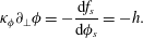 $$\begin{eqnarray}\unicode[STIX]{x1D705}_{\unicode[STIX]{x1D719}}\unicode[STIX]{x2202}_{\bot }\unicode[STIX]{x1D719}=-\frac{\text{d}f_{s}}{\text{d}\unicode[STIX]{x1D719}_{s}}=-h.\end{eqnarray}$$
The value of the parameter
 $h$
(the surface excess chemical potential) is related to the equilibrium contact angle
 $\unicode[STIX]{x1D703}^{eq}$
via (Briant & Yeomans Reference Briant and Yeomans2004)
 $$\begin{eqnarray}h=\sqrt{2\unicode[STIX]{x1D705}_{\unicode[STIX]{x1D719}}A}\text{ sign }\left[\frac{\unicode[STIX]{x03C0}}{2}-\unicode[STIX]{x1D703}^{eq}\right]\sqrt{\cos \left(\frac{\unicode[STIX]{x1D6FC}}{3}\right)\left\{1-\cos \left(\frac{\unicode[STIX]{x1D6FC}}{3}\right)\right\}},\end{eqnarray}$$
where
 $\unicode[STIX]{x1D6FC}=\arccos (\sin ^{2}\unicode[STIX]{x1D703}^{eq})$
and the function sign returns the sign of its argument.
This choice of the free energy leads to the chemical potential
 $$\begin{eqnarray}\unicode[STIX]{x1D707}=\frac{\unicode[STIX]{x1D6FF}{\mathcal{F}}}{\unicode[STIX]{x1D6FF}\unicode[STIX]{x1D719}}=-A\unicode[STIX]{x1D719}+A\unicode[STIX]{x1D719}^{3}-\unicode[STIX]{x1D705}_{\unicode[STIX]{x1D719}}\unicode[STIX]{x2202}_{\unicode[STIX]{x1D6FE}\unicode[STIX]{x1D6FE}}\unicode[STIX]{x1D719},\end{eqnarray}$$
and the pressure tensor (Anderson, McFadden & Wheeler Reference Anderson, McFadden and Wheeler1998)
 $$\begin{eqnarray}\unicode[STIX]{x1D617}_{\unicode[STIX]{x1D6FC}\unicode[STIX]{x1D6FD}}=\left[p_{b}-\unicode[STIX]{x1D705}_{\unicode[STIX]{x1D719}}\unicode[STIX]{x1D719}\unicode[STIX]{x2202}_{\unicode[STIX]{x1D6FE}\unicode[STIX]{x1D6FE}}\unicode[STIX]{x1D719}-\frac{\unicode[STIX]{x1D705}_{\unicode[STIX]{x1D719}}}{2}(\unicode[STIX]{x2202}_{\unicode[STIX]{x1D6FE}}\unicode[STIX]{x1D719})^{2}\right]\unicode[STIX]{x1D6FF}_{\unicode[STIX]{x1D6FC}\unicode[STIX]{x1D6FD}}+\unicode[STIX]{x1D705}_{\unicode[STIX]{x1D719}}(\unicode[STIX]{x2202}_{\unicode[STIX]{x1D6FC}}\unicode[STIX]{x1D719})(\unicode[STIX]{x2202}_{\unicode[STIX]{x1D6FD}}\unicode[STIX]{x1D719}),\end{eqnarray}$$
where
 $p_{b}=(c^{2}/3)\unicode[STIX]{x1D70C}-(A\unicode[STIX]{x1D719}^{2})/2+(3/4)A\unicode[STIX]{x1D719}^{4}$
is the bulk pressure.
2.2.2 Equations of motion
The hydrodynamic equations for the system are the continuity, (2.7), and the Navier–Stokes, (2.8), equations for a non-ideal fluid
 $$\begin{eqnarray}\displaystyle & \displaystyle \unicode[STIX]{x2202}_{t}\unicode[STIX]{x1D70C}+\unicode[STIX]{x2202}_{\unicode[STIX]{x1D6FC}}(\unicode[STIX]{x1D70C}u_{\unicode[STIX]{x1D6FC}})=0, & \displaystyle\end{eqnarray}$$
 $$\begin{eqnarray}\displaystyle & \displaystyle \unicode[STIX]{x2202}_{t}(\unicode[STIX]{x1D70C}u_{\unicode[STIX]{x1D6FC}})+\unicode[STIX]{x2202}_{\unicode[STIX]{x1D6FD}}(\unicode[STIX]{x1D70C}u_{\unicode[STIX]{x1D6FC}}u_{\unicode[STIX]{x1D6FD}})=-\unicode[STIX]{x2202}_{\unicode[STIX]{x1D6FD}}\unicode[STIX]{x1D617}_{\unicode[STIX]{x1D6FC}\unicode[STIX]{x1D6FD}}+\unicode[STIX]{x2202}_{\unicode[STIX]{x1D6FD}}[\unicode[STIX]{x1D702}(\unicode[STIX]{x2202}_{\unicode[STIX]{x1D6FD}}u_{\unicode[STIX]{x1D6FC}}+\unicode[STIX]{x2202}_{\unicode[STIX]{x1D6FC}}u_{\unicode[STIX]{x1D6FD}})], & \displaystyle\end{eqnarray}$$
where
 $\boldsymbol{u}$
,
 $\unicode[STIX]{x1D64B}$
,
 $\unicode[STIX]{x1D702}$
are the fluid velocity, pressure tensor and dynamic viscosity respectively. For a binary fluid the equations of motion are coupled with a convection–diffusion equation,
 $$\begin{eqnarray}\unicode[STIX]{x2202}_{t}\unicode[STIX]{x1D719}+\unicode[STIX]{x2202}_{\unicode[STIX]{x1D6FC}}(\unicode[STIX]{x1D719}u_{\unicode[STIX]{x1D6FC}})=M\unicode[STIX]{x1D6FB}^{2}\unicode[STIX]{x1D707},\end{eqnarray}$$
that describes the dynamics of the order parameter
 $\unicode[STIX]{x1D719}$
.
 $M$
is a mobility coefficient.
2.2.3 Lattice Boltzmann method
The equations of motion are solved using a standard free energy lattice Boltzmann algorithm for a binary fluid (Briant & Yeomans Reference Briant and Yeomans2004). In particular we use a three-dimensional model with 19 discrete velocity vectors (D3Q19) and adopt a multiple relaxation time (MRT) (D’Humières et al.
Reference D’Humières, Ginzburg, Krafczyk, Lallemand and Luo2002) approach for the evolution of the distribution functions,
 $f_{i}$
, associated with the fluid density
 $\unicode[STIX]{x1D70C}$
. Following Pooley, Kusumaatmaja & Yeomans (Reference Pooley, Kusumaatmaja and Yeomans2009), the relaxation times responsible for generating the viscous terms in the Navier–Stokes equation are set to
 $\unicode[STIX]{x1D70F}_{f}$
(based on the fluid viscosity
 $\unicode[STIX]{x1D702}=\unicode[STIX]{x1D70C}(\unicode[STIX]{x1D70F}_{f}-0.5)/3$
), those related to conserved quantities to infinity and all the others, which correspond to non-hydrodynamic modes, to unity. A single relaxation time approach is sufficient for the order parameter
 $\unicode[STIX]{x1D719}$
. The relaxation time for the evolution of the distribution functions,
 $g_{i}$
, associated with the concentration
 $\unicode[STIX]{x1D719}$
is set to
 $\unicode[STIX]{x1D70F}_{g}=1$
. As shown by Pooley et al. (Reference Pooley, Kusumaatmaja and Yeomans2009), this approach suppresses spurious currents at the contact line, while improving significantly the numerical stability of the algorithm as well (Lallemand & Luo Reference Lallemand and Luo2000). For a detailed description of the lattice Boltzmann (LB) implementation we refer the reader to (Briant & Yeomans Reference Briant and Yeomans2004; Yeomans Reference Yeomans2006; Pooley et al.
Reference Pooley, Kusumaatmaja and Yeomans2008, Reference Pooley, Kusumaatmaja and Yeomans2009).
Numerically we solve the equations of motion using graphics processing units (NVIDIA Tesla K40 GPU cards), taking advantage of the fact that the LB method is particularly well suited for computations on a parallel architecture (Gray, Cen & Boek Reference Gray, Cen and Boek2016). Running the simulations in parallel on 8 Tesla K40 cards reduces the required computational time to a few days for the most computationally intensive simulation.
3 Results and discussion
In this section we will present our results. We start with primary drainage, which also serves as a validation for our experiments. Then we turn our attention to the imbibition case, where we examine pore filling events and investigate the role of pore geometry in determining the displacement pathways.
Quasi-static primary drainage images in a micro-model (Geometry 2) with etch depth
 $d=45~\unicode[STIX]{x03BC}\text{m}$
and throat widths
 $w_{t}$
: 33, 51, 65,
 $107~\unicode[STIX]{x03BC}\text{m}$
(WP-white, NWP-grey). Contact angle
 $26^{\circ }$
.

Critical pressures for drainage in a micro-model (Geometry 2) with etch depth
 $d=45~\unicode[STIX]{x03BC}\text{m}$
and unequal throat widths
 $w_{t}$
: 33, 51, 65 and
 $107~\unicode[STIX]{x03BC}\text{m}$
, calculated via (1.1) and experimental data. Contact angle:
 $26^{\circ }$
, interfacial tension:
 $0.024~\text{N}~\text{m}^{-1}$
. Experimental error of
 $\pm 7$
Pa is attained by the 1 mm accuracy the height of the reservoir can be set to.

3.1 Primary drainage
The model was initially filled with the WP. For the quasi-static displacement, the
 $P_{w}$
was gradually decreased, allowing the NWP to enter the largest throat first, before sequentially displacing the WP from the throats in decreasing size order, as can be seen in figure 3. This type of displacement is referred to as ‘piston-type’ motion (Lenormand et al.
Reference Lenormand, Zarcone and Sarr1983), when the NWP enters the throat filled with the WP only if the capillary pressure is equal to or greater than a given value
 $P_{p}=P_{nw}-P_{w}=2\unicode[STIX]{x1D6FE}\cos \unicode[STIX]{x1D703}^{eq}(1/d+1/w_{t})$
, which we call ‘the critical pressure’. The calculated theoretical and experimental critical pressures for drainage within the throats are displayed in table 1. Generally there is good agreement between the two.
For the dynamic drainage, the NWP is injected into the chip at a constant flow rate of
 $0.5~\unicode[STIX]{x03BC}\text{l}~\text{min}^{-1}$
. This leads to the displacement of the WP at a constant mean velocity
 $u$
in each throat, prior to and after the square pore body. The corresponding capillary number for the interface motion in the throat prior to the pore body is
 $Ca=\unicode[STIX]{x1D702}_{w}u/\unicode[STIX]{x1D6FE}\sim 10^{-4}$
. Typical values for the ratio of viscous to capillary forces at the pore scale, quantified by the capillary number, are in the range of
 $10^{-3}$
–
 $10^{-10}$
, depending on the distance from the injection point in the well bore (Blunt & Scher Reference Blunt and Scher1995). Again, as can be seen in figure 4(a), the NWP displaces the WP via the largest downstream throat first, as predicted by (1.1). To validate the displacement sequence, we have carried out LB simulations in exactly the same geometry, the same value for
 $Ca$
and contact angle as in the experiment. The fluid flow was driven by applying velocity boundary conditions (Hecht & Harting Reference Hecht and Harting2010) at the inlet and outlet of the simulation domain to match the experimental conditions. The results are presented in figure 4(b) and display a good agreement with the experimental displacement sequence.
3.2 Imbibition
3.2.1 Quasi-static imbibition
Pore-filling events are dependent on the number of throats connected to the pore that are occupied with the NWP along with their orientation. Generally, pore-filling events are designated as
 $I_{1}$
,
 $I_{2}$
,
 $I_{3}\ldots I_{n}$
, with
 $n$
indicating the number of throats filled with the NWP (Lenormand et al.
Reference Lenormand, Zarcone and Sarr1983). Here
 $I_{1,2,2A,3}$
pore-filling events were investigated via quasi-static imbibition experiments, by gradually increasing
 $P_{w}$
, in a micro-model with equal throat widths (Geometry 1: etch depth
 $d=56~\unicode[STIX]{x03BC}\text{m}$
, throat width
 $w_{t}=73~\unicode[STIX]{x03BC}\text{m}$
, pore width
 $238~\unicode[STIX]{x03BC}\text{m}$
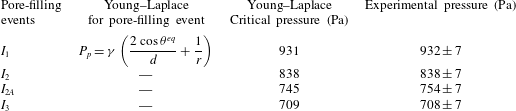
), see figure 5. At a critical capillary pressure the WP spontaneously displaces the NWP via ‘piston-type’ displacement. In all cases the critical pressure of the pore-filling event calculated from the Young–Laplace equation is very close to the experimentally determined critical pressure, as shown in table 2. Good agreement is achieved as we know the exact pore geometry and can observe the meniscus shape, allowing the critical radii to be well defined, as illustrated for each case in figure 5.
Primary dynamic drainage images: (a) experimental images of forced injection of NWP at
 $0.5~\unicode[STIX]{x03BC}\text{l}~\text{min}^{-1}$
. (b) Corresponding LB simulations. The dashed arrow denotes the direction of the flow.

Quasi-static
 $I_{1}$
,
 $I_{2}$
,
 $I_{2A}$
and
 $I_{3}$
imbibition experimental results (WP – white, NWP – grey). The critical radii in the plane of the micro-model,
 $r_{2}=r$
, used to calculate the displacement pressures for each case are also illustrated together with
 $r_{1}=d/2\cos \unicode[STIX]{x1D703}^{eq}$
.

Critical pressures for each pore-filling event in a micro-model (Geometry 1) with equal throat widths. Contact angle:
 $28^{\circ }$
, etch depth
 $d=56~\unicode[STIX]{x03BC}\text{m}$
, throat width
 $w_{t}=73~\unicode[STIX]{x03BC}\text{m}$
, pore width:
 $238~\unicode[STIX]{x03BC}\text{m}$
, interfacial tension:
 $0.024~\text{N}~\text{m}^{-1}$
. The critical radii in the plane of the micro-model
 $r_{2}=r$
used in the calculation of the critical pressures is shown in figure 5. The principal radii of curvature, equation (1.1), are
 $r_{1}=d/2\cos \unicode[STIX]{x1D703}^{eq},r_{2}=r$
. Experimental error of
 $\pm 7$
Pa is attained by the 1 mm accuracy the height of the reservoir can be set to.
Quasi-static experiments were also conducted in a micro-model (Geometry 3) with unequal throats (etch depth
 $d=55~\unicode[STIX]{x03BC}\text{m}$
, throat widths
 $w_{t}=27$
, 47, 60,
 $100~\unicode[STIX]{x03BC}\text{m}$
pore: 155,
 $236~\unicode[STIX]{x03BC}\text{m}$
). The predicted displacement sequence for this geometry, using the Young–Laplace equation and a contact angle of
 $16^{\circ }$
, is first snap off (
 $P_{s}$
) in the narrowest throat at 1240 Pa, followed by pore body filling via ‘piston-type’ displacement (
 $P_{p}$
) at 869 Pa, see figure 6(a). The snap-off pressure,
 $P_{s}=2\unicode[STIX]{x1D6FE}(\cos \unicode[STIX]{x1D703}^{eq}-\sin \unicode[STIX]{x1D703}^{eq})/\min (d,w_{t})$
, was estimated from the pressure at which two growing corner menisci meet on the channel wall (Valvatne & Blunt Reference Valvatne and Blunt2004). Snap off is able to occur during the quasi-static experiments, as there is time for the advancing WP films to develop ahead of the main meniscus, which swell and become unstable (Bico & Quéré Reference Bico and Quéré2003; Kavehpour et al.
Reference Kavehpour, Ovryn and McKinley2003), see figure 6(b), and because ‘piston-type’ displacement is not possible for topological reasons (Lenormand et al.
Reference Lenormand, Zarcone and Sarr1983). The WP films can be clearly seen in figure 7 as the darker lines outlining the model geometry.
(a) Predicted displacement sequence for quasi-static
 $I_{3}$
imbibition (Geometry 3) using the Young–Laplace equation for a contact angle of
 $16^{\circ }$
, with the narrowest throat filling first via snap off (
 $P_{s}$
), followed by the body filling through piston-like displacement (
 $P_{p}$
). (b) Schematic illustration of the snap-off mechanism. Swelling of the corner WP films leads to snap off when the menisci meet on the channel wall (dashed line) and become unstable. Top panel: configuration in the plane of the micro-model at the channel wall. Bottom panel: cross-sectional view in the orthogonal plane.

Quasi-static
 $I_{3}$
imbibition experimental results (WP – white, NWP – grey, wetting films – black). Snap off occurs in the narrowest throat before the meniscus enters the pore as predicted by the Young–Laplace equation.

Spontaneous
 $I_{3}$
imbibition experimental results ((a), Geometry 3, throat widths: (
 $T_{1}$
)
 $w_{t}=27~\unicode[STIX]{x03BC}\text{m}$
, (
 $T_{2}$
)
 $w_{t}=47~\unicode[STIX]{x03BC}\text{m}$
, (
 $T_{3}$
)
 $w_{t}=60~\unicode[STIX]{x03BC}\text{m}$
, (
 $T_{4}$
)
 $w_{t}=100~\unicode[STIX]{x03BC}\text{m}$
, etch depth
 $d=55~\unicode[STIX]{x03BC}\text{m}$
), with the corresponding LB simulations (b); here the WP travels down the adjacent throat first. This behaviour is not predicted by the Young–Laplace law (1.1). Equilibrium contact angle
 $\unicode[STIX]{x1D703}^{eq}=16^{\circ }$
, viscosity ratio
 $r_{\unicode[STIX]{x1D702}}=\unicode[STIX]{x1D702}_{w}/\unicode[STIX]{x1D702}_{nw}=50$
.

3.2.2 Spontaneous imbibition
Extending our research to spontaneous imbibition, we investigated the
 $I_{3}$
displacement mechanism, which was compared to LB simulations, figure 8. During our spontaneous imbibition experiments we observed that the advancing meniscus did travel down an adjacent throat (
 $T_{2}$
) first instead of filling the smallest throat, as the WP films do not have time to develop ahead of the advancing meniscus. Indeed, Lenormand (Reference Lenormand1990) noted that when no wetting films are present along the corners of the models, the imbibing WP should enter an adjacent throat first, but no direct evidence was provided. Here we confirm this hypothesis directly and show our results in a series of snapshots from experiment and corresponding LB simulations in figure 8. Thus, displacement does not occur in the order predicted by the Young–Laplace equation. This is understandable as all the downstream throats have lower critical entry pressures than the pore body. Therefore, as soon as the critical pore-filling pressure has been exceeded, the WP can enter any of the downstream throats. Hence, in the case of spontaneous imbibition, the pore body geometry becomes a key factor in determining in which order the downstream throats will fill.
Capillary-filling dynamics in a rectangular throat
A reasonable assumption then could be that the dynamics of imbibition in the throat prior to the junction (
 $T_{3}$
) may affect the pore filling sequence and the selection of the displacement pathway. Hence, we turn our attention to the imbibition dynamics. We recently (Zacharoudiou & Boek Reference Zacharoudiou and Boek2016) examined the dynamics of capillary filling in two-dimensional channels and covered both: (i) the limit of long times for both high and low viscosity ratios
 $r_{\unicode[STIX]{x1D702}}=\unicode[STIX]{x1D702}_{w}/\unicode[STIX]{x1D702}_{nw}$
and (ii) the limit of short times, demonstrating that the free energy LB method can capture the correct dynamics for the process. We recall that in the limit of high viscosity ratios and long times, when the total time is much larger than the viscous time scale
 $t_{v}\sim \unicode[STIX]{x1D70C}L_{s}^{2}/\unicode[STIX]{x1D702}_{w}$
(Quéré Reference Quéré1997; Stange, Dreyer & Rath Reference Stange, Dreyer and Rath2003), the Lucas–Washburn regime (
 $l\sim sqrt(t)$
) (Lucas Reference Lucas1918; Washburn Reference Washburn1921) is expected. In the limit of short times two regimes, namely (i) inertial regime (
 $l\sim t^{2}$
) and (ii) visco–inertial regime (
 $l\sim t$
) can precede the Lucas–Washburn regime (Dreyer et al.
Reference Dreyer, Delgado and Path1994; Stange et al.
Reference Stange, Dreyer and Rath2003). The hydraulic diameter
 $D_{h}=2dw_{t}/(d+w_{t})$
is used as the characteristic length scale
 $L_{s}$
for evaluating
 $t_{v}$
.
Ichikawa, Hosokawa & Maeda (Reference Ichikawa, Hosokawa and Maeda2004) examined the interface motion driven by capillary action in the case of three-dimensional channels with a rectangular cross-section. Using the analytical solution of Brody, Yager & Austin (Reference Brody, Yager, Goldstein and Austin1996) for the velocity profile in a rectangular channel of aspect ratio
 $\unicode[STIX]{x1D716}=d/w_{t}$
and balancing the relevant forces, they estimated the dimensionless relation for the interface position as a function of time
 $$\begin{eqnarray}l^{\ast 2}=\cos \unicode[STIX]{x1D703}^{eq}(t^{\ast }-1+\text{e}^{-t^{\ast }}).\end{eqnarray}$$
The rescaled time and length are defined as
 $t^{\ast }=t/t_{c}$
and
 $l^{\ast }=l/l_{c}$
respectively, where
 $$\begin{eqnarray}t_{c}=\frac{8\unicode[STIX]{x1D716}^{2}\left[1-\displaystyle \frac{2\unicode[STIX]{x1D716}}{\unicode[STIX]{x03C0}}\tanh \left(\displaystyle \frac{\unicode[STIX]{x03C0}}{2\unicode[STIX]{x1D716}}\right)\right]}{\unicode[STIX]{x03C0}^{4}}\times t_{v},\quad l_{c}=2t_{c}\sqrt{\frac{(1+\unicode[STIX]{x1D716})\unicode[STIX]{x1D6FE}}{\unicode[STIX]{x1D716}\unicode[STIX]{x1D70C}w_{t}}}.\end{eqnarray}$$
(a) Length of the penetrating fluid column in throat
 $T_{3}$
for simulations with varying viscosity ratio
 $r_{\unicode[STIX]{x1D702}}=\unicode[STIX]{x1D702}_{w}/\unicode[STIX]{x1D702}_{nw}$
as a function of time in lattice units (l.u.). What appears as a deviation from the
 $l\sim t^{2}$
regime at early times (first point for
 $r_{\unicode[STIX]{x1D702}}=5$
) is due to the interface retracting initially in the connected reservoir which can result in interfacial oscillations (Stange et al.
Reference Stange, Dreyer and Rath2003; Zacharoudiou & Boek Reference Zacharoudiou and Boek2016). (b) Length versus time in scaled units according to (3.2). The theoretical prediction of Ichikawa et al. (Reference Ichikawa, Hosokawa and Maeda2004), equation (3.1), is given with the dashed line.

Here, we first compare our results with the theoretical prediction of Ichikawa et al. (Reference Ichikawa, Hosokawa and Maeda2004), equation (3.1), before examining whether the capillary-filling dynamics affects the displacement pathway after the junction. We considered equilibrium contact angles of
 $\unicode[STIX]{x1D703}^{eq}=30^{\circ }$
and
 $16^{\circ }$
(experimental condition). Starting with a situation with a high viscosity ratio
 $r_{\unicode[STIX]{x1D702}}=\unicode[STIX]{x1D702}_{w}/\unicode[STIX]{x1D702}_{nw}=500$
by choosing relaxation rates
 $\unicode[STIX]{x1D70F}_{f,w}=1.5$
and
 $\unicode[STIX]{x1D70F}_{f,nw}=0.502$
, we decrease the viscosity ratio to
 $r_{\unicode[STIX]{x1D702}}=5$
by decreasing
 $\unicode[STIX]{x1D702}_{w}$
, while
 $\unicode[STIX]{x1D702}_{nw}$
is kept fixed. This choice decreases the rate of viscous dissipation in the WP as the viscosity ratio decreases from
 $r_{\unicode[STIX]{x1D702}}=500$
to
 $r_{\unicode[STIX]{x1D702}}=5$
, allowing for more energy to be available to the interface motion as it enters the junction region.
Figure 9(a) shows the length of the penetrating WP column in throat
 $T_{3}$
for simulations with varying viscosity ratio
 $r_{\unicode[STIX]{x1D702}}$
and
 $\unicode[STIX]{x1D703}^{eq}=30^{\circ }$
. In the limit of long times and high viscosity ratios the Lucas–Washburn regime (
 $l\sim sqrt(t)$
) (Lucas Reference Lucas1918; Washburn Reference Washburn1921) is clearly observed. The viscous time scale
 $t_{v}$
is of the order of
 $10^{4}$
in lattice units (l.u.) for
 $r_{\unicode[STIX]{x1D702}}=25,50$
, thus enabling us to also obtain the
 $l\sim t^{2}$
regime at early times, as the interface accelerates initially penetrating the throat. This initial acceleration of the interface for
 $r_{\unicode[STIX]{x1D702}}=5,25$
and 50 is reflected in the increasing dynamic contact angle
 $\unicode[STIX]{x1D703}_{xz}^{\unicode[STIX]{x1D6FC}}$
, shown in figure 10(a).
(a) Time variation of the dynamic contact angle in the
 $xz$
plane (etch depth direction)
 $\unicode[STIX]{x1D703}_{xz}^{\unicode[STIX]{x1D6FC}}$
for the imbibition process in throat
 $T_{3}$
. The behaviour of
 $\unicode[STIX]{x1D703}_{xy}^{\unicode[STIX]{x1D6FC}}$
is the same. The increase observed in
 $\unicode[STIX]{x1D703}_{xz}^{\unicode[STIX]{x1D6FC}}$
at the end of each simulation set is due to the interface reaching the end of throat
 $T_{3}$
and entering the junction region. The equilibrium value of the contact angle
 $\unicode[STIX]{x1D703}^{eq}=30^{\circ }$
(dashed line). (b) The cosine of
 $\unicode[STIX]{x1D703}_{xz}^{\unicode[STIX]{x1D6FC}}$
plotted against the capillary number
 $Ca$
. Results affected by the interface approaching the junction region were excluded. The solid lines correspond to linear fits of each data set to
 $Ca$
to enable comparison with the theoretical prediction of Cox (Reference Cox1986), Sheng & Zhou (Reference Sheng and Zhou1992), equation (3.3). (c) Illustration of the WP column configuration, as it imbibes throat
 $T_{3}$
, and the definition for the dynamic contact angle.

Rescaling length and time using (3.2) reveals that our numerical results approach the theoretical prediction of Ichikawa et al. (Reference Ichikawa, Hosokawa and Maeda2004), equation (3.1), in the limit of long times as shown in figure 9(b). Here we used the equilibrium value of the contact angle
 $\unicode[STIX]{x1D703}^{eq}=30^{\circ }$
, although actually the dynamic contact angle, shown in figure 10(a), varies with time as it depends on the interfacial velocity and
 $Ca$
(Cox Reference Cox1986; Sheng & Zhou Reference Sheng and Zhou1992). Using the dynamic contact angle instead would decrease slightly
 $l^{\ast }$
improving the agreement further. The dynamic contact angle, in the
 $xy$
and
 $xz$
planes, is evaluated by fitting the interface in the central region of the advancing meniscus to a circle, as shown in figure 10(c). The angle of intersection this circle makes with the side walls is
 $\unicode[STIX]{x1D703}_{xy,xz}^{\unicode[STIX]{x1D6FC}}$
.
Figure 10(b) depicts the variation of
 $\cos (\unicode[STIX]{x1D703}_{xz}^{\unicode[STIX]{x1D6FC}})$
as a function of the capillary number
 $Ca$
. This is in agreement with the theoretical predicted dependency of
 $\unicode[STIX]{x1D703}_{xz}^{\unicode[STIX]{x1D6FC}}$
on
 $Ca$
(Cox Reference Cox1986; Sheng & Zhou Reference Sheng and Zhou1992)
 $$\begin{eqnarray}\cos \unicode[STIX]{x1D703}^{\unicode[STIX]{x1D6FC}}=\cos \unicode[STIX]{x1D703}^{eq}-Ca\ln (KL_{s}/l_{s}).\end{eqnarray}$$
 $K$
is a fitting constant,
 $L_{s}$
is a characteristic length scale of the system and
 $l_{s}$
is the effective slip length at the contact line. High interfacial velocities translate to high
 $\unicode[STIX]{x1D703}_{xz}^{\unicode[STIX]{x1D6FC}}$
, while as the interface slows down
 $\unicode[STIX]{x1D703}_{xz}^{\unicode[STIX]{x1D6FC}}$
approaches the equilibrium value
 $\unicode[STIX]{x1D703}^{eq}$
. Fitting the results for each simulation set to (3.3) and extrapolating to
 $Ca=0$
reveals the following
 $\unicode[STIX]{x1D703}_{Ca=0}^{\unicode[STIX]{x1D6FC}}=29.2^{\circ },30.3^{\circ },30.9^{\circ }$
and
 $29.4^{\circ }$
for
 $r_{\unicode[STIX]{x1D702}}=5,25,50$
and 500 respectively. Hence, this verifies that the dynamic contact angle tends to the correct value for the equilibrium contact angle of
 $\unicode[STIX]{x1D703}^{eq}=30^{\circ }$
. The deviation increases for the case of
 $\unicode[STIX]{x1D703}^{eq}=16^{\circ }$
and is of the order of a few degrees (
 ${\sim}5^{\circ }$
). This is expected for very small or large contact angles due to the finite width of the interface and has been observed for binary and ternary systems as well (Pooley et al.
Reference Pooley, Kusumaatmaja and Yeomans2009; Semprebon, Krüger & Kusumaatmaja Reference Semprebon, Krüger and Kusumaatmaja2016).
We next examined the velocity of the interface front. Decreasing the viscosity ratio by decreasing the viscosity of the WP results in less viscous dissipation in the WP and hence more energy becomes available for driving the interface in the channel. Figure 11(a) shows the corresponding
 $Ca=\unicode[STIX]{x1D702}_{w}u/\unicode[STIX]{x1D6FE}$
. The experimental
 $Ca$
is of the order of
 $10^{-2}$
(
 $r_{\unicode[STIX]{x1D702}}\sim 50$
). Ichikawa et al. (Reference Ichikawa, Hosokawa and Maeda2004) estimated the dimensionless velocity
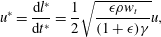 $$\begin{eqnarray}u^{\ast }=\frac{\text{d}l^{\ast }}{\text{d}t^{\ast }}=\frac{1}{2}\sqrt{\frac{\unicode[STIX]{x1D716}\unicode[STIX]{x1D70C}w_{t}}{(1+\unicode[STIX]{x1D716})\unicode[STIX]{x1D6FE}}}u,\end{eqnarray}$$
which, in the limit of long times, approaches
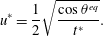 $$\begin{eqnarray}u^{\ast }=\frac{1}{2}\sqrt{\frac{\cos \unicode[STIX]{x1D703}^{eq}}{t^{\ast }}}.\end{eqnarray}$$
Although they neglected variations in the advancing dynamic contact angle
 $\unicode[STIX]{x1D703}^{\unicode[STIX]{x1D6FC}}$
, equation (3.5) can still be considered valid in the limit of long times as the advancing contact angle
 $\unicode[STIX]{x1D703}^{\unicode[STIX]{x1D6FC}}$
approaches the equilibrium value
 $\unicode[STIX]{x1D703}^{eq}$
. It is evident that the numerical results demonstrate excellent agreement with the theoretical prediction of Ichikawa et al. (Reference Ichikawa, Hosokawa and Maeda2004) (figure 11
b).
(a) The capillary number,
 $Ca=\unicode[STIX]{x1D702}_{w}u/\unicode[STIX]{x1D6FE}$
, for the interface front motion in throat
 $T_{3}$
as a function of time (in l.u.) for varying
 $r_{\unicode[STIX]{x1D702}}$
and
 $\unicode[STIX]{x1D703}^{eq}=30^{\circ }$
. At the end of throat
 $T_{3}$
the velocity decreases significantly, as the interface enters the junction region. (b) Interfacial velocity and time in scaled units. The theoretical prediction of Ichikawa et al. (Reference Ichikawa, Hosokawa and Maeda2004), equation (3.5), is given with the dashed line.

Junction region
Having validated the interface motion in the throat prior to the junction, we next examine the interface motion in the wider pore body. As the interface approaches the end of throat
 $T_{3}$
and enters the junction region, it decelerates at first as the driving capillary forces per unit area decrease and the interface adapts a concave shape in the
 $xy$
-plane. This reduction in the interfacial velocity is evident in figure 11. On the other hand inertial forces can keep the interface moving in the junction, while the motion is opposed by viscous forces that can damp this forward movement. Hence, an important dimensionless number that can affect the dynamics of the interface entering the junction is the Ohnesorge number
 $$\begin{eqnarray}Oh=\frac{\unicode[STIX]{x1D702}_{w}}{\sqrt{\unicode[STIX]{x1D70C}\unicode[STIX]{x1D6FE}L_{s}}},\end{eqnarray}$$
which gives the relative importance of viscous forces over inertial and capillary forces. Inertial forces (per unit volume), which scale as
 ${\sim}\unicode[STIX]{x1D70C}u^{2}/L_{s}$
, are in the range
 $10^{-6}$
(
 $r_{\unicode[STIX]{x1D702}}=5$
)–
 $10^{-9}$
(
 $r_{\unicode[STIX]{x1D702}}=500$
) in l.u. Viscous forces (per unit volume), which scale as
 ${\sim}\unicode[STIX]{x1D702}_{w}u/L_{s}^{2}$
, are in the range
 $10^{-8}$
in l.u. for all cases as
 $r_{\unicode[STIX]{x1D702}}$
increases from 5 to 500. Capillary forces
 $F_{cap}=2\unicode[STIX]{x1D6FE}\cos \unicode[STIX]{x1D703}^{\unicode[STIX]{x1D6FC}}(d+w_{t})$
are of the order of 1 in l.u. for all cases.
On a second stage, the contact line in the
 $xy$
-plane makes contact with the side walls, see figure 12(a). As this favours energetically a transition from a concave to a convex configuration (dashed yellow line to the solid black line configuration), the surface energy released and the interface configuration transition can lead to interfacial oscillations, which, as demonstrated in figure 12(b), are more profound with decreasing
 $Oh$
. Time is normalised by the time
 $t_{cont}$
when the interface imbibes throat
 $T_{2}$
. Similar interfacial oscillations have been observed by Ferrari & Lunati (Reference Ferrari and Lunati2013), who examined a forced imbibition situation. Here we demonstrate that these oscillations can be generated as the interface travels through a narrow throat to a wider pore body in a spontaneous imbibition scenario as well, due to the small
 $Oh$
, with the mechanism behind this being the same. As the interface progresses further in the junction, the kinetic energy that was available is gradually dissipated and the forward movement is due to the action of capillary filling. This becomes more clear when looking at the interface configuration in the junction at a level
 $z=d/2$
for viscosity ratios
 $r_{\unicode[STIX]{x1D702}}=5$
(
 $Oh=6\times 10^{-3}$
) and
 $r_{\unicode[STIX]{x1D702}}=50$
(
 $Oh=6\times 10^{-2}$
), figure 13.
(a) Interface configuration in the
 $xy$
-plane at
 $z=d/2$
as the interface enters the junction region. When the contact line makes contact with the side walls the interface configuration can change from concave to convex leading to interfacial oscillations. (b) Velocity of the interface (in l.u.) measured along the dashed line shown in figure 13 for simulations with varying
 $r_{\unicode[STIX]{x1D702}}$
and Ohnesorge number (
 $Oh$
). Interfacial oscillations are evident, especially as
 $Oh$
decreases. Results are plotted as a function of dimensionless time
 $t^{\ast }=t/t_{cont}$
, where time is normalised by the time
 $t_{cont}$
when the interface imbibes throat
 $T_{2}$
.

Interface configuration in the
 $xy$
-plane (
 $z=d/2$
) in the junction for (a)
 $r_{\unicode[STIX]{x1D702}}=5$
,
 $Oh=6\times 10^{-3}$
and (b)
 $r_{\unicode[STIX]{x1D702}}=50$
,
 $Oh=6\times 10^{-2}$
.

Figure 14(a) shows the length travelled by the meniscus in the junction, measured along the dashed line in figure 13, for varying
 $r_{\unicode[STIX]{x1D702}}$
and
 $Oh$
. The similar shape of the curves, with two peaks – labelled as (1) and (3) – and two troughs – points (2) and (4) – is due to the transition from a concave to convex configuration, favoured by the shape of the junction. As expected, increasing the viscosity of the wetting phase (increasing
 $r_{\unicode[STIX]{x1D702}}$
) increases the time it takes for the interface to imbibe into the next downstream throat,
 $t_{cont}$
. For all situations examined here, the fluid imbibes throat
 $T_{2}$
first, which is achieved when the interface has progressed a length
 $l\sim 85$
in the junction region. In other words, geometry dictates the pore-filling sequence, irrespective of the dynamics prior to the selection of the next downstream throat or the filling rules proposed by Lenormand et al. (Reference Lenormand, Zarcone and Sarr1983). The same is observed for the simulations reported in figure 14(b), which examines simulations with the same viscosity ratio (
 $r_{\unicode[STIX]{x1D702}}=50$
) and different
 $Oh$
, achieved by varying the viscosity of both phases. We note here that the capillary number is approximately the same in these simulations (
 $Ca\sim 8\times 10^{-4}$
);
 $t_{cont}$
varies significantly though as can be clearly observed, as a consequence of the different rates at which energy is dissipated in the system. Therefore, an important remark here is that
 $Ca$
itself is not sufficient to characterise the fluid flow. The dimensionless numbers, relevant to the specific type of fluid flow, must be matched, for example the viscosity ratio
 $r_{\unicode[STIX]{x1D702}}$
and the
 $Oh$
, in order to characterise the fluid flow dynamics.
Junction region: (a) length versus time (in l.u.) for varying viscosity ratios
 $r_{\unicode[STIX]{x1D702}}$
, measured along the line shown in figure 13(a). The wetting fluid starts imbibing the next downstream throat (
 $T_{2}$
) when
 $l\sim 85$
and
 $t=t_{cont}$
. (b) Simulation results with
 $r_{\unicode[STIX]{x1D702}}=50$
and different
 $Oh$
, by varying the viscosities of both phases. Increasing fluids’ viscosities increases
 $Oh$
and
 $t_{cont}$
. The average
 $Ca=\unicode[STIX]{x1D702}_{w}\bar{u}/\unicode[STIX]{x1D6FE}$
for the interface motion in the junction is
 $8.1\times 10^{-4}$
(
 $Oh=6\times 10^{-2}$
),
 $8.4\times 10^{-4}$
(
 $Oh=2\times 10^{-1}$
) and
 $7.9\times 10^{-4}$
(
 $Oh=1\times 10^{0}$
). The labels (0)–(4) correspond to the snapshots in figure 13(b). Inset: the moment the wetting phase starts imbibing the throat
 $T_{2}$
(
 $t=t_{cont}$
) the interface retracts in the middle of the junction (reduction in
 $l$
).

Examining the imbibition process in the junction in terms of the surface energies, and given that we kept all parameters fixed except for the fluid viscosities, we note that the surface energy released, due to wetting, and used to drive the fluid–fluid interface, is the same for all runs. What changes is the rate of viscous dissipation,
 $$\begin{eqnarray}\unicode[STIX]{x1D6F7}=2\int _{V}\unicode[STIX]{x1D702}_{i}\dot{\unicode[STIX]{x1D750}}_{\unicode[STIX]{x1D6FC}\unicode[STIX]{x1D6FD}}\dot{\unicode[STIX]{x1D750}}_{\unicode[STIX]{x1D6FC}\unicode[STIX]{x1D6FD}}\,\text{d}V>0,\end{eqnarray}$$
which dictates how much energy is left available as kinetic energy for the fluid motion.
 $\unicode[STIX]{x1D702}_{i}$
(
 $i=w,nw$
) is the local viscosity and
 $\dot{\unicode[STIX]{x1D750}}_{\unicode[STIX]{x1D6FC}\unicode[STIX]{x1D6FD}}=(\unicode[STIX]{x2202}_{\unicode[STIX]{x1D6FC}}u_{\unicode[STIX]{x1D6FD}}+\unicode[STIX]{x2202}_{\unicode[STIX]{x1D6FD}}u_{\unicode[STIX]{x1D6FC}})/2$
is the rate of strain tensor. For the spontaneous imbibition situation we examine here, the energy balance states (Ferrari & Lunati Reference Ferrari and Lunati2013)
 $$\begin{eqnarray}\frac{\text{d}E_{k}}{\text{d}t}=-\frac{\text{d}F}{\text{d}t}-\unicode[STIX]{x1D6F7},\end{eqnarray}$$
where
 $E_{k}$
and
 $F$
are the kinetic energy and surface free energy respectively. In figure 15(a) the viscous dissipation rate is plotted as a function of time for two of the simulations reported in figure 14(b), covering the interface motion both in throat
 $T_{3}$
(prior the junction) and in the junction region. In figure 15(b) viscous dissipation rate in dimensionless form
 $\unicode[STIX]{x1D6F7}^{\ast }=\unicode[STIX]{x1D6F7}/\unicode[STIX]{x1D6FE}D_{h}\bar{u}$
is plotted as a function of dimensionless time
 $t^{\ast }=t/t_{cont}$
. As the viscosity of both fluids increases to maintain the same
 $r_{\unicode[STIX]{x1D702}}$
, the total amount of energy dissipated (area under the curves, i.e.
 $\int \unicode[STIX]{x1D6F7}\,\text{d}t$
) increases, and hence the change in kinetic energy decreases. The peak which is clearly visible for each case, corresponds to time
 $t=t_{cont}$
, when the wetting fluid starts imbibing throat
 $T_{2}$
, resulting in an increase in the fluid velocity.
(a) Viscous dissipation rate as a function of time (in l.u.) for the simulations reported in figure 14(b). This covers the fluid–fluid interface motion in the throat
 $T_{3}$
(
 $t\leqslant t_{1}$
) and in the junction region (
 $t\geqslant t_{1}$
). The corresponding values of viscosities are
 $\unicode[STIX]{x1D702}_{w}=8.33\times 10^{-2}$
,
 $\unicode[STIX]{x1D702}_{nw}=1.67\times 10^{-3}$
(
 $Oh=2\times 10^{-1}$
) and
 $\unicode[STIX]{x1D702}_{w}=6.67\times 10^{-1}$
,
 $\unicode[STIX]{x1D702}_{nw}=1.33\times 10^{-2}$
(
 $Oh=1\times 10^{0}$
). (b) Viscous dissipation rate versus time in scaled units.

The change in the total surface energy can be expressed as
 $$\begin{eqnarray}\text{d}F=\unicode[STIX]{x1D6FE}\,\text{d}A_{int}+\unicode[STIX]{x1D6FE}_{ws}\,\text{d}A_{ws}+\unicode[STIX]{x1D6FE}_{ns}\,\text{d}A_{ns},\end{eqnarray}$$
where
 $\text{d}A_{int}$
,
 $\text{d}A_{ws}$
and
 $\text{d}A_{ns}$
are the increments of the areas of the fluid–fluid, solid–wetting phase fluid and solid–non-wetting phase fluid interfaces respectively and
 $\unicode[STIX]{x1D6FE}$
,
 $\unicode[STIX]{x1D6FE}_{ws}$
,
 $\unicode[STIX]{x1D6FE}_{ns}$
the corresponding surface tensions. Given that the total solid surface area
 $A_{tot}^{s}=A_{ns}+A_{ws}$
is constant and that
 $\text{d}A_{ns}=-\text{d}A_{ws}$
, then
 $$\begin{eqnarray}\text{d}F=\unicode[STIX]{x1D6FE}(\text{d}A_{int}-\cos \unicode[STIX]{x1D703}^{eq}\,\text{d}A_{ws}).\end{eqnarray}$$
The total surface energy is given by
 $F=\unicode[STIX]{x1D6FE}(A_{int}-\cos \unicode[STIX]{x1D703}^{eq}A_{ws})+F_{0}$
, where
 $F_{0}=\unicode[STIX]{x1D6FE}_{ns}A_{tot}^{s}$
is constant. Plotting
 $F-F_{0}$
as a function of dimensionless time
 $t^{\ast }=t/t_{cont}$
in figure 16(a), reveals that the total surface energy decreases monotonically. It also demonstrates that the released energy is approximately the same for all simulations, as expected.
(a) The total surface energy
 $F-F_{0}$
(in l.u.) as a function of dimensionless time
 $t^{\ast }=t/t_{cont}$
in the junction region for varying viscosity ratios
 $r_{\unicode[STIX]{x1D702}}$
. The energy released from wetting the solid surfaces (
 $\text{d}F<0$
) drives the fluid inside the micro-model geometry. (b) The area of the fluid–fluid interface (in l.u.). This is measured using the marching cubes algorithm.

Wetting film growth in the side throats, along the dashed lines, for the simulations reported in figures 14(b) and 15 with
 $r_{\unicode[STIX]{x1D702}}=50$
and (a)
 $Oh=2\times 10^{-1}$
, (b)
 $Oh=1\times 10^{0}$
. A situation with higher viscous dissipation rate (b) decreases the amount of energy converted to kinetic energy and hence the mean velocity along the
 $x$
-direction. This gives more time for the development of thin wetting films progressing along the corners of the micro-channel. The snapshots correspond at the same length travelled in the
 $x$
-direction and approximately at the same normalised time
 $t^{\ast }=t/t_{cont}$
.

Finally, an interesting feature was observed when comparing situations with the same viscosity ratio (
 $r_{\unicode[STIX]{x1D702}}=50$
), see figure 14(b). The longer times
 $t_{cont}$
observed, as viscous dissipation (and
 $Oh$
) increases, allow more time to the interface to progress along the corners of the side throats. This is shown in figure 16(b), where we plot the area of the fluid–fluid interface as well as in figure 17, where we show snapshots of the interface configuration in the junction. In a complex geometry, as in porous media, swelling of these films and the consequent collapse can affect the displacement pathways. Especially in porous media and natural rock formations the effective diameter varies continuously with length, favouring filling of the narrowest downstream throat as predicted by the filling rules of Lenormand et al. (Reference Lenormand, Zarcone and Sarr1983). Here, however, and examining a wide range of parameters relevant to spontaneous imbibition dynamics, LB simulations revealed that the pore-filling sequence remained the same, with the pore geometry being the major influencing factor.
4 Conclusions
It was observed that for both the drainage and quasi-static imbibition experiments the displacement pathways predicted by the Young–Laplace law are obeyed. LB simulations also followed these displacement predictions for drainage. In addition, the theoretical critical pressures for displacement events were in good agreement with calculated experimental events. For our spontaneous imbibition experiments, on the other hand, we found that the WP enters an adjacent throat first due to the absence of WP film growth. Lenormand (Reference Lenormand1990) suggested that the imbibing WP should enter an adjacent throat first, but no direct evidence was provided. Here we confirm this hypothesis, for the first time, directly using experiment and corresponding LB simulations. Thus, pore geometry plays a vital role as it becomes the main deciding factor in the displacement pathways. Once the critical pressure of the pore has been exceeded, all downstream throats are able to be filled. This displacement choice was observed in both our spontaneous imbibition experiments, and the corresponding LB simulations for models of the same geometry. The implications of the absence of WP films within the models have not been investigated.
Furthermore, we observe that the displacement of the meniscus in a throat and the scaling of the imbibing fluid column with time can fall in the early time flow regimes of capillary filling ((i)
 $l\sim t^{2}$
, (ii)
 $l\sim t$
) prior the Lucas–Washburn regime ((iii)
 $l\sim sqrt(t)$
). An in-depth investigation of imbibition dynamics using lattice Boltzmann simulations was carried out in Zacharoudiou & Boek (Reference Zacharoudiou and Boek2016). We emphasise here that matching the relevant dimensionless numbers is essential in correctly resolving the multiphase flow dynamics, as
 $Ca$
itself is not sufficient to uniquely describe the flow. For example, we need to match the viscosity ratio and the Ohnesorge number, which for fluid flow at the pore scale is typically
 $Oh\ll 1$
. Nevertheless, for the range of parameters examined here, LB simulations revealed that the pore-filling sequence remained the same. Therefore, the main message of the current paper is that the filling order of channels connected to a junction depends primarily on the geometry of the pore body and is largely independent of the details of the dynamic meniscus shape influenced by inertial effects.
In addition to the above, in real porous media, microscopic WP films can develop under strong wetting conditions and flow through the cervices and the micro-roughness of the pore walls, whereas in our micro-fluidic devices WP films develop at the right-angled wedges. This, however, will not change the main message of the current paper. Several papers in the literature have discussed the development of thin WP films in porous media, including Vizika, Avraam & Payatakes (Reference Vizika, Avraam and Payatakes1994), Constantinides & Payatakes (Reference Constantinides and Payatakes2000), Bico & Quéré (Reference Bico and Quéré2003). Depending on the time scales associated with the general advancement of the fluid–fluid interface (
 $t_{adv}$
) and the time scales for thin films to develop and swell (
 $t_{film}$
), the displacement pathways can be very different. If the fluid flow is fast, for example in the manuscript the spontaneous imbibition situation (
 $t_{film}>t_{adv}$
), then the displacement pathway is mainly affected by the geometry. On the other hand, if the fluid flow is very slow (providing time for thin films to develop and swell), for example in the manuscript the quasi-static imbibition situation (
 $t_{film}<t_{adv}$
), then the displacement pathway and the pore-filling sequence is likely to follow the filling rules proposed by Lenormand et al. (Reference Lenormand, Zarcone and Sarr1983), based on the Young–Laplace equation.
The advancement of the invading WP fluid in a real porous medium, under strong wetting conditions, involves two distinct macroscopic fronts (Constantinides & Payatakes Reference Constantinides and Payatakes2000; Bico & Quéré Reference Bico and Quéré2003). The primary displacement front, which saturates the medium, is due to the piston-type motion of menisci in the main pores. The secondary front is due to the precursor WP films, which propagate ahead of the primary front using the fine structures of the porous material. The distance between the two fronts depends on the capillary number
 $Ca$
and the viscosity ratio and may be many times larger than the mean pore length (Constantinides & Payatakes Reference Constantinides and Payatakes2000). Under certain conditions the WP films can swell and cause disconnection and entrapment of the NWP. In these situations the displacement pathways can be significantly different from situations with no WP films. The impact of this phenomenon can be significant. For example Constantinides & Payatakes (Reference Constantinides and Payatakes2000) report that these WP films cause a substantial increase of the residual NWP saturation. Rücker et al. (Reference Rücker, Berg, Armstrong, Georgiadis, Ott, Schwing, Neiteler, Brussee, Makurat and Leu2015) report on regimes of corner flow and film swelling in real porous media, decreasing the connectivity of the NWP. Micro-fluidic devices and simulations can be used to investigate the dynamics and mechanisms involved in two phase flow at the pore scale and elucidate the role of wettability, viscosity ratio,
 $Ca$
or even roughness using patterned micro-fluidic devices on the advancement of the displacement fronts.
Acknowledgements
This work was conducted as part of the Qatar Carbonates and Carbon Storage Research Centre (QCCSRC), jointly funded by Qatar Petroleum, Shell and the Qatar Science and Technology Park. E.M.C. would also like to acknowledge the Engineering and Physical Sciences Research Council (EPSRC) for their funding.


 Open access

