


1. Introduction
The idea that tariffs can increase the levying country’ s welfare dates back to the 1820s and the writings of Robert Torrens and J. S. Mill (see Irwin, Reference Irwin1996). The rigorous proof of the idea’s validity was not completed until the end of that century, when neoclassical economists such as Marshall and Edgeworth invented the reciprocal demand techniques and indifference curve analysis and applied them to the barter model of trade, assuming perfect wage flexibility and full employment.Footnote 1 However, domestic unemployment often justifies use of tariffs. Can the tariff really create jobs when a country suffers from chronic unemployment? In 1930, more than 1,000 economists did not think so and urged President Hoover to veto the Smoot-Hawley Tariff Act.Footnote 2 In 1931, however, J.M. Keynes advocated for a uniform tariff on all imports to combat the deflation that was ravaging the U.K. economy under the gold standard (Eichengreen, Reference Eichengreen1984).
The controversy about the tariff and job creation continues today. A case in point is President Trump’s April 2025 declaration of a national emergency and sweeping tariffs at a baseline rate of 10% on all imports and higher reciprocal rates on countries with significant trade surpluses with the U.S.
Given this historic background, this paper aims to reexamine the question raised by Keynes (Reference Keynes1936): can the tariff pull a country out of stagnation? To address this question, we present a model that integrates real and monetary aspects of international trade. The real (or barter) model of trade draws on Dornbusch, Fischer, and Samuelson (DFS for short, Reference Dornbusch, Fischer and Samuelson1977). Thus, the model has two countries producing a continuum of goods with labor under linear technologies and trading according to the Ricardian comparative advantage. This model has an obvious advantage over the standard two-good model in that it allows an examination of the effect of tariffs on industry output (intensive margins) and destruction and creation of industries in each country (extensive margins).Footnote 3
To incorporate monetary variables into our analysis, we extend the closed-country secular stagnation model developed by Ono (Reference Ono1994, Reference Ono2001) to an international setting. Thus, we assume consumers maximize their lifetime utility by choosing real consumption and real money balances at each instant, and the marginal utility of real money balance holdings is bounded below by a positive value. As we show below, the latter assumption can give rise to a liquidity trap and chronic unemployment. We also assume nominal wages adjust sluggishly under unemployment but perfectly flexible under full employment. All other markets including one for international assets clear instantaneously.Footnote 4
We use the integrated model to examine the effect of a tariff on the terms of trade, the trade pattern, and the levels of real consumption and employment. With the possibility of unemployment in both countries, there are three equilibrium outcomes to consider: (i) full employment in both countries, (ii) unemployment in both countries, (iii) unemployment in one and full employment in the other. In all these cases we assume the exchange rates are completely flexible.
We now summarize our findings. First, in our model the classical result holds in all three cases, i.e., the imposition of a tariff increases the country’s relative real wage (the terms of trade). The tariff also shrinks the range of each country’s exports, a result familiar from the DFS model. Second, the imposition of a tariff also yields results that depend crucially on the country’s labor market conditions. For instance, if the country has full employment, the imposition of a small tariff increases its real consumption (and keeps full employment) but affects the foreign country differently, depending on the latter’s labor conditions. If foreign labor is fully employed, the foreign country’s real consumption declines with the deteriorating terms of trade. If instead foreign labor is unemployed, falling prices expand demands for foreign goods and as a consequence foreign consumption and employment increase.
We next turn to the case in which the country suffers from chronic unemployment. We find that the imposition of a small tariff decreases the country’s real consumption and increases joblessness. This contrasts sharply with the Keynes’s prescription for a tariff. The effect of a home tariff on the foreign economy again depends on its employment condition. If foreign labor is fully employed, deteriorating the terms of trade cause foreign real consumption to decline. If foreign labor is unemployed, however, a deterioration in the terms of trade makes foreign goods cheaper. Expanding demand for foreign goods increases jobs and real consumption in the foreign economy.
Furthermore, the quantitative analysis reveals the following implications of large tariff changes. Under full employment, the relationship between tariffs and consumption is inverted U-shaped: higher tariffs increase consumption at low initial tariff levels, whereas they reduce consumption at high tariff levels. In contrast, under stagnation, the relationship is U-shaped: higher tariffs reduce consumption at low tariff levels but increase consumption at high tariff levels.
Having summarized our main findings, we next relate our work to the relevant literature. The DFS model, like ours, incorporates monetary aspects of trade into the Ricardian model. However, they do so through the quantity theory of money. Despite this difference, a tariff affects the home country’s economy in the same way under full employment and flexible exchange rates; namely, a tariff improves its terms of trade, increases its real consumption and narrows the range of its exports. In the presence of unemployment, however, the results diverge between the two models. The DFS model ascribes unemployment to strict nominal wage rigidity. Given the constant velocity of money, the supply of national money completely determines the employment level. In such a setting a tariff causes an equiproportional appreciation of the home currency to countervail the rise in its relative wage but has no effect on employment.
Like us, Ono (Reference Ono2014) addresses the tariff question within a monetary model. However, he assumes two goods in the Ricardian framework. Thus, his analysis does investigate the tariff’s effect on the intensive margin of trade. However, in trade data, the extensive margin of trade (product varieties) is known to play a more significant role than the intensive margin (Broda and Weinstein, Reference Broda and Weinstein2006). Ono’s analysis is also limited to the symmetric cases (full employment or unemployment in both countries). Our analysis extends his work to asymmetric case. Finally, we also investigate the effects of large tariff changes numerically. Specifically, we show the way symmetric economies can transition into asymmetric economies, depending on each country’ s tariff policy. This type of transition analysis provides a novel perspective and clearly distinguishes our work from Ono (Reference Ono2014).Footnote 5
There is also much work investigating the effect of tariffs in pure monetary models. For example, Mundell (Reference Mundell1966) utilized a framework, which would later turn into the Mundell-Fleming model, to find that under flexible exchange rates with nominal wage rigidity a tariff causes a depreciation of the levying country’ s money and a reduction in quantities of its output and employment. Eichengreen (Reference Eichengreen1983) showed that Mundell’s finding holds even with downward real wage rigidity if the tariff revenues are rebated to domestic consumers in a lump-sum fashion. These models are static and also lack microfoundations. In recent years researchers studied macroeconomic fluctuations within an open-economy version of the RBC and DSGE frameworks (Obstfeld and Rogoff, Reference Obstfeld and Rogoff1996; Galí and Monacelli, Reference Galí and Monacelli2005; and Uribe and Schmitt-Grohé, Reference Uribe and Schmitt-Grohé2017). These researchers have focused on business fluctuations due to various shocks around a full-employment steady state. More recently, Naito (Reference Naito2021) used an endogenous growth model under the lab-equipment specification and found the cases where optimal tariffs can be zero even for a large country. Bergin and Corsetti (Reference Bergin and Corsetti2023) considered a model with international production chains and investigated the optimal monetary response to exogenous tariff policy shocks. Iwaisako and Tanaka (Reference Iwaisako and Tanaka2026) used a dynamic North-South model with foreign direct investment to show that northern tariffs can shift production back to the North, increase labor costs, and slow growth, while southern tariffs encourage production in the South, lower northern labor costs, and boost growth. These studies, however, assume full employment.Footnote 6
The remainder of this paper proceeds as follows. Section 2 outlines the model. Section 3 examines the effects of tariffs on the terms of trade, the trade pattern (the extensive margins), real consumption, and employment under flexible exchange rates. Section 4 calibrates the model and numerically simulates the impact of tariff changes. The final section summarizes our findings and concludes the paper.
2. The model
We consider the continuous-time model with two countries, which we call the home and the foreign country. For the remainder of the paper, we omit the time notation
 $t$
unless ambiguities arise. The real side of the model is based on the Ricardian model from DFS (Reference Dornbusch, Fischer and Samuelson1977). There is a continuum of goods, which are indexed by
 $i$
and arranged on the unit interval
 $[0,1]$
.
2.1. Firms
A typical home firm can produce
 $y(i)$
units of good
 $i$
by employing
 $l(i)$
units of home labor under the Ricardian technology:
 \begin{equation*} y(i)=\frac {1}{a(i)}l(i), \end{equation*}
where
 $a(i)$
denotes the constant unit labor requirement for good
 $i\in [0,1]$
. The home firm’s objective is to maximize its profit,
 $P(i)y(i)-Wl(i)$
, for given nominal price
 $P(i)$
and nominal wage
 $W$
. The first-order condition gives
 \begin{equation*} P(i)=a(i)W \quad \mathrm{if}\;y(i)\gt 0,{ \ \;\ }P(i)\lt a(i)W \quad \mathrm{if}\;y(i)=0. \end{equation*}
If good
 $i$
is produced in the home country, we have
 \begin{equation} \frac {P(i)}{P}\equiv p(i)=a(i)w, \end{equation}
where
 $P$
is the nominal price index,
 $p(i)$
is the real price of good
 $i$
, and
 $w({\equiv} W/P)$
is the real wage in the home country. Similar relations hold in the foreign country. If we let the asterisk (*) denote the corresponding foreign variables, we can write the ratio of the home wage to the foreign wage as
 \begin{equation} \omega \equiv \dfrac {W}{\varepsilon W^{\ast }}=\dfrac {w}{w^{\ast }}\dfrac {P}{\varepsilon P^{\ast }}, \end{equation}
where
 $\varepsilon$
is the nominal exchange rate (the home currency price of the foreign exchange).
Let
 $A(i)$
denote the relative productivity of home labor for good
 $i$
. Rearrange the goods in order of decreasing home country productivity so that the derivative
 $A'(i)$
is negative, that is,
 \begin{equation} A(i)\equiv \frac {a^{*}(i)}{a(i)};\quad A^{\prime }(i)\lt 0,\quad i\in \left [0,1\right ]\!. \end{equation}
This implies that the home country specializes in producing goods with lower indices
 $i\in [0,I]$
whereas the foreign country specializes in higher-indexed goods
 $[I^{*},1]$
. For the two borderline goods
 $I$
and
 $I^{*}$
, the domestic price equals the trade cost-adjusted import price:
 \begin{eqnarray*} \text{Home products }i & \in & [0,I]\text{: }\quad P(I)=(1+\tau )\xi \varepsilon P^{\ast }(I),\\ \text{Foreign products }i & \in & [I^{\ast },1]\text{: }\quad P^{\ast }(I^{\ast })=(1+\tau ^{\ast })\xi \frac {P(I^{\ast })}{\varepsilon }, \end{eqnarray*}
where
 $\xi (\geq 1)$
is the iceberg trade cost (Samuelson, Reference Samuelson1954), and
 $\tau$
and
 $\tau ^{*}$
are the uniform ad valorem tariff rates on the CIF (Cost, Insurance, and Freight) basis. By applying (1) and (2) to these conditions, we find that
 $I$
and
 $I^{*}$
satisfy these relations:
 \begin{equation} A(I)=z\equiv \frac {\omega }{(1+\tau )\xi },\quad A(I^{\ast })=z^{*}\equiv (1+\tau ^{\ast })\xi \omega . \end{equation}
From (4),
 $z$
,
 $z^{*}$
,
 $I$
, and
 $I^{\ast }$
satisfy
 \begin{equation} z^{*}\geq z,\quad I({=}\, A^{-1}(z))\geq I^{\ast }({=}\, A^{-1}(z^{*})). \end{equation}
Equation (5) indicates that firms in two countries face different relative prices due to transportation costs and tariffs. As a result, the two countries produce different sets (numbers of industries) of goods. The goods
 $i\in \left [I^{\ast },I\right ]$
are produced in both countries and hence not traded.
Consumers in each country buy domestic goods (
 $i\in [0,I]$
in home and
 $i\in [I^{*},1]$
in foreign) and imported goods (
 $i\in [I,1]$
in home and
 $i\in [0,I^{*}]$
in foreign). From (1) and (4), consumers in each country face the real prices as below:
 \begin{align} \text{Home:} \text{}\,p(i)&=\begin{cases} a(i)w \quad \text{for }i\in \left [0,A^{-1}(z)\right]\!,\\[4pt] \dfrac {a^{\ast }(i)w}{z}\quad \text{for }i\in \left [A^{-1}(z),1\right ]\!, \end{cases}\nonumber \\[3pt] \text{Foreign:} \text{ }\,p^{*}(i)&=\begin{cases} z^{*}a(i)w^{*}\quad \text{for }i\in \left [0,A^{-1}(z^{*})\right]\!,\\[4pt] a^{*}(i)w^{*}\quad \text{for }i\in \left [A^{-1}(z^{*}),1\right ]\!. \end{cases} \end{align}
2.2. Consumers
We let
 $L$
and
 $L^{*}$
denote the numbers of consumers in the home and foreign country, respectively. Each consumer is endowed with one unit of labor. We use notation
 $({}^*)$
to avoid repetitions for each country.
Each consumer is infinitely lived and obtains instantaneous utilities
 $u^{(*)}(c^{(*)})$
by consuming the consumption index
 $c^{(*)}$
defined below and
 $v^{(*)}(m^{(*)})$
by holding real money balances
 $m^{(*)}$
. A consumer’s lifetime utility is given by
 \begin{equation} U^{(*)}=\int _{0}^{\infty }\left (u^{(*)}(c^{(*)})+v^{(*)}(m^{(*)})\right )\exp ({-}\rho t)dt, \end{equation}
where
 $\rho$
is the common subjective discount rate. The consumption index is defined by
 \begin{equation} c^{(*)}=\left (\int \nolimits _{0}^{1}c^{(*)}(i)^{\frac {\sigma -1}{\sigma }}di\right )^{\frac {\sigma }{\sigma -1}},\;\;\;\sigma \gt 1, \end{equation}
where
 $c^{(*)}(i)$
is individual demand for good
 $i$
and
 $\sigma$
stands for the elasticity of substitution. The instantaneous utility functions,
 $u^{(*)}(c^{(*)})$
and
 $v^{(*)}(m^{(*)})$
, satisfy
 \begin{equation*} u^{(*)\prime }\gt 0,\quad \lim _{c^{(*)}\rightarrow \infty }u^{(*)\prime }(c^{(*)})=0,\quad u^{(*)\prime \prime }\lt 0, \end{equation*}
 \begin{equation} v^{(*)\prime }\gt 0,\quad \lim _{m^{(*)}\rightarrow \infty }v^{(*)\prime }(m^{(*)})=\beta ^{(*)}\gt 0,\quad v^{(*)\prime \prime }\leq 0, \end{equation}
where
 $\beta ^{(*)}$
is a positive constant. The marginal utility of real balances
 $v^{(*)\prime }(m^{(*)})$
is bounded away from zero but
 $u^{(*)}(c^{(*)})$
satisfies the Inada condition. These properties play a key role in creating persistent demand shortages; see Section 3.
Given the specialization patterns by (4), consumers determine
 $c^{(*)}(i)$
to maximize (8) subject to the nominal expenditure
 $E^{(*)}$
:
 \begin{eqnarray} E({=}\,Pc) & = & \int \nolimits _{0}^{I}P(i)c(i)di+\int \nolimits _{I}^{1}(1+\tau )\xi \varepsilon P^{\ast }(i)c(i)di,\nonumber \\ E^{\ast }({=}\,P^{\ast }c^{*}) & = & \int _{0}^{I^{\ast }}(1+\tau ^{\ast })\xi \frac {P(i)}{\varepsilon }c^{\ast }(i)di+\int _{I^{\ast }}^{1}P^{\ast }(i)c^{\ast }(i)di, \end{eqnarray}
which gives the individual demand
 $c(i)$
and
 $c^{*}(i)$
for good
 $i$
:
 \begin{equation} c(i)=p(i)^{-\sigma }c,\quad c^{*}(i)=p^{*}(i)^{-\sigma }c^{*}. \end{equation}
Dividing both sides of (10) by price indices
 $P^{(\ast )}$
, using (6) and (11), and rearranging the result, we can express the real wages as follows (see Appendix A for detail):
 \begin{align} w=w(z)&\equiv \Bigg (\int _{0}^{A^{-1}(z)}a(i)^{-(\sigma -1)}di+z^{\sigma -1}\int _{A^{-1}(z)}^{1}a^{*}(i)^{-(\sigma -1)}di\Bigg)^{\frac {1}{\sigma -1}},\nonumber \\ w^{\ast }=w^{\ast }(z^{*})&\equiv \Bigg (z^{*}{}^{-(\sigma -1)}\int _{0}^{A^{-1}(z^{*})}a(i)^{-(\sigma -1)}di+\int _{A^{-1}(z^{*})}^{1}a^{\ast }(i)^{-(\sigma -1)}di\Bigg )^{\frac {1}{\sigma -1}}. \end{align}
Let
 $\delta ^{(*)}$
denote the fraction of income home (or foreign) consumers spend on home goods. Then we can apply (6), (11) and (12) to write
 \begin{equation*} \delta =\frac {\int _{0}^{A^{-1}(z)}p(i)c(i)di}{c}=\frac {\int _{0}^{A^{-1}(z)}a(i)^{-(\sigma -1)}di}{\int _{0}^{A^{-1}(z)}a(i)^{-(\sigma -1)}di+z^{\sigma -1}\int _{A^{-1}(z)}^{1}a^{*}(i)^{-(\sigma -1)}di}\equiv \hat {\delta }(z), \end{equation*}
 \begin{equation} \delta ^{*}=\frac {\int _{0}^{A^{-1}(z^{*})}p(i)c(i)di}{c^{*}}=\frac {\int _{0}^{A^{-1}(z^{\ast })}a(i)^{-(\sigma -1)}di}{\int _{0}^{A^{-1}(z^{\ast })}a(i)^{-(\sigma -1)}di+z^{\ast }{}^{(\sigma -1)}\int _{A^{-1}(z^{\ast })}^{1}a^{\ast }(i)^{-(\sigma -1)}di}\equiv \hat {\delta }(z^{*}), \end{equation}
from which with (5) we obtain
 \begin{equation*} \hat {\delta }^{\prime }\lt 0,\quad \delta \geq \delta ^{*}, \end{equation*}
which implies that home consumers spend a larger fraction of their incomes on home-produced goods than foreigners do. Note also that the relative price elasticity of
 $w^{(\ast )}$
in (12) satisfies
 \begin{equation} \frac {w^{\prime }z}{w}=1-\delta ,\quad \frac {w^{*\prime }z^{*}}{w^{*}}=-\delta ^{*}. \end{equation}
Each consumer is endowed with one unit of labor time. Then, each consumer receives wage income
 $w^{(*)}x^{(*)}$
, where
 $x^{(\ast )}\in [0,1]$
is the actual employment of labor per capita. This is because the actual employment is determined on the short side of the labor market. Each consumer allocates its total asset (
 $b^{(*)}$
) between international lending and borrowing assets (
 $f^{(*)}$
) and real money balances (
 $m^{(*)}$
). This gives the following flow and stock budget constraints expressed in real terms:
 \begin{eqnarray} \dot {b} & = & rb+wx-c-Rm+s,\quad b=m+f,\nonumber \\ \dot {b}^{\ast } & = & r^{\ast }b^{\ast }+w^{\ast }x^{\ast }-c^{\ast }-R^{\ast }m^{\ast }+s^{\ast },\quad b^{\ast }=m^{\ast }+f^{\ast }, \end{eqnarray}
where
 $r^{(*)}$
is the real interest rate,
 $R^{(*)}$
is the nominal interest rate,
 $s^{(\ast )}$
is a lump-sum subsidy (or tax if negative), and a dot denotes time differentiation.Footnote
7
To keep things simple, initial international asset holdings (i.e., initial debts) are assumed to be zero.Footnote
8
Thus,
 \begin{equation} f_{0}=0,\quad f_{0}^{*}=0. \end{equation}
The real and nominal interest rates on international assets,
 $r^{(\ast )}$
and
 $R^{(\ast )}$
, satisfy
 \begin{equation} R=r+\pi ,\quad R^{\ast }=r^{\ast }+\pi ^{\ast }, \end{equation}
where
 $\pi ^{(\ast )}\equiv \dot {P}^{(\ast )}/P^{(\ast )}$
. The non-arbitrage condition on international assets gives
 \begin{equation} R=\frac {\dot {\varepsilon }}{\varepsilon }+R^{\ast }. \end{equation}
Each consumer’s objective is to maximize (7) subject to the budget constraints. The current-value Hamiltonian of a home consumer is given by:
 \begin{equation*} H=u(c)+v(m)+\varsigma (rb+wx-c-Rm+s), \end{equation*}
where
 $\varsigma$
is the costate variable for
 $b$
. Maximization of the Hamiltonian yields the first-order optimality conditions:
 \begin{equation*} u^{\prime }(c)=\varsigma ,\quad v^{\prime }(m)=\varsigma R,\quad \dot {\varsigma }=(\rho -r)\varsigma . \end{equation*}
Since a foreign consumer’s behavior is similarly described, from the above conditions we obtain the following Euler equation and money demand equation:
 \begin{equation*} \eta ^{(*)}\frac {\dot {c}^{(*)}}{c^{(*)}}=r^{(*)}-\rho ,\quad R^{(*)}=\frac {v^{(*)\prime }(m^{(*)})}{u^{(*)\prime }(c^{(*)})}, \end{equation*}
where
 $\eta ^{(\ast )}\equiv -u^{(*)\prime \prime }(c^{(*)})c^{(*)}/u^{(*)\prime }(c^{(*)})$
is the elasticity of marginal utility with respect to consumption
 $c^{(*)}$
. Using (17), the above equations can be summarized as follows:
 \begin{equation} \eta ^{(*)}\frac {\dot {c}^{(*)}}{c^{(*)}}+\rho +\pi ^{(*)}=R^{(*)}=\frac {v^{(*)\prime }(m^{(*)})}{u^{(*)\prime }(c^{(*)})}. \end{equation}
The transversality condition is satisfied when
 \begin{equation*} \lim _{t\rightarrow \infty }\varsigma b\exp ({-}\rho t)=0,\quad \lim _{t\rightarrow \infty }\varsigma ^{\ast }b^{\ast }\exp ({-}\rho t)=0. \end{equation*}
2.3. Governments
Suppose that the home (foreign) government imposes a tariff on imported goods and rebates the tax revenue equally to all residents in a lump-sum fashion. Then each government’s lump-sum subsidy
 $s^{(\ast )}$
is
 \begin{equation} s=\frac {\tau }{1+\tau }(1-\delta )c,\quad s^{*}=\frac {\tau ^{\ast }}{1+\tau ^{\ast }}\delta ^{*}c^{\ast }. \end{equation}
The nominal money supply
 $M^{S(\ast )}$
is assumed to be held constant throughout the analysis.
2.4. Market adjustments
Given the consumer, firm, and government behaviors discussed above, the money and international asset markets adjust perfectly and instantaneously to ensure that the following conditions hold continuously:Footnote 9
 \begin{equation} \text{Money markets:}\quad mL=\frac {M^{S}}{P},\quad m^{\ast }L^{\ast }=\frac {M^{S\ast }}{P^{\ast }}, \end{equation}
 \begin{equation} \text{International asset market:}\quad fL+\frac {\varepsilon P^{*}}{P}f^{\ast }L^{\ast }=0, \end{equation}
where
 $M^{S(\ast )}$
represents the nominal money supply. The good market adjustment is also assumed to be perfect; hence,
 \begin{align*} \frac {l(i)}{a(i)}\left ({=}\,y(i)\right )&=\begin{cases} c(i)L+\xi c^{\ast }(i)L^{\ast } & \mbox{for }i\in [0,I^{\ast }],\\ c(i)L & \mbox{for }i\in [I^{\ast },I], \end{cases} \\[6pt]\frac {l^{\ast }(i)}{a^{\ast }(i)}\left ({=}\,y^{\ast }(i)\right )&=\begin{cases} c^{\ast }(i)L^{\ast } & \mbox{for }i\in [I^{\ast },I],\\ \xi c(i)L+c^{\ast }(i)L^{\ast } & \mbox{for }i\in [I,1]. \end{cases} \end{align*}
In contrast, the labor market is segmented internationally. The nominal wage adjustment is perfect if full employment prevails but sluggish if there is unemployment. Thus, the wage adjustment is the following:
 \begin{align} \mbox{When } x^{(\ast )}&=1, \quad \mbox{wages are perfectly adjusted};\nonumber \\ \mbox{When } x^{(\ast )}&\lt 1, \quad \frac {\dot {W}^{(*)}}{W^{(\ast )}}=\alpha ^{(\ast )}(x^{(\ast )}-1), \end{align}
where
 $\alpha ^{(\ast )}$
represents the adjustment speed of the nominal wage
 $W^{(\ast )}$
when there is unemployment.Footnote
10
Because total revenues equal total labor costs under linear technology and perfect competition, and
 $\delta ^{(\ast )}$
is each country’s expenditure ratio on the goods produced by the home country, we have
 \begin{align*} W\int _{0}^{I}l(i)di&=\int _{0}^{I}P(i)y(i)di=P\delta cL+\varepsilon P^{\ast }\frac {\delta ^{*}c^{\ast }}{(1+\tau ^{*})}L^{\ast }, \\ W^{\ast }\int _{I^{*}}^{1}l^{\ast }(i)di&=\int _{I^{*}}^{1}P^{*}(i)y^{*}(i)di=\left (\frac {P}{\varepsilon }\right )\frac {(1-\delta )c}{(1+\tau )}L+P^{\ast }(1-\delta ^{*})c^{\ast }L^{\ast }. \end{align*}
Therefore, using (2) and (4), we find the employment rate
 $x^{(\ast )}$
to equal
 \begin{align} x&=\frac {\int _{0}^{I}l(i)di}{L}=\frac {\delta c}{w}+\left (\frac {L^{\ast }}{L}\right )\frac {\xi \delta ^{*}c^{\ast }}{z^{*}w^{\ast }},\nonumber\\x^{\ast }&=\frac {\int _{I^{*}}^{1}l^{\ast }(i)di}{L^{\ast }}=\left (\frac {L}{L^{\ast }}\right )\frac {z\xi (1-\delta )c}{w}+\frac {(1-\delta ^{*})c^{\ast }}{w^{\ast }}. \end{align}
Given that the money supply is constant in each country, Equation (21) allows us to represent changes in
 $m^{(\ast )}$
by the differential equation
 \begin{equation} \frac {\dot {m}^{(\ast )}}{m^{(\ast )}}=-\pi ^{(\ast )}. \end{equation}
Each country’s current account per capita
 $CA^{(*)}$
generates international asset dynamics per capita
 $\dot {f}^{(*)}$
, which can be expressed, after substituting (20) and (25) into the budget Equation (15), as
 \begin{align} \dot {f}&=CA=rf+wx-\frac {1+\tau \delta }{1+\tau }c,\nonumber\\\dot {f}^{*}&=CA^{*}=r^{*}f^{\ast }+w^{\ast }x^{\ast }-\frac {1+\tau ^{\ast }(1-\delta ^{*})}{1+\tau ^{\ast }}c^{\ast }. \end{align}
For clarity, Table 1 summarizes the definitions of the variables and parameters used in the subsequent analysis.
Notation summary

Table 1. Long description
The table has two columns: Notation and Variables/Parameters. It contains 35 rows, each defining a variable or parameter. Row 1: Notation, ε; Variables/Parameters, Nominal exchange rate. Row 2: Notation, W (W*); Variables/Parameters, Nominal wage rate: Home (Foreign). Row 3: Notation, P (P*); Variables/Parameters, Price index: Home (Foreign). Row 4: Notation, ω ≡ W/εW*; Variables/Parameters, Relative wage. Row 5: Notation, y(i); Variables/Parameters, Production of good i. Row 6: Notation, l(i); Variables/Parameters, Labor demand for y(i). Row 7: Notation, A(i) ≡ α(i)/α(macron i); Variables/Parameters, Relative unit labor requirement. Row 8: Notation, p(i) ≡ P(i)/P (p*(i) ≡ P*(i)/P*); Variables/Parameters, Real price of Home (Foreign) good i. Row 9: Notation, τ (τ*); Variables/Parameters, Home (Foreign) tariff. Row 10: Notation, ξ; Variables/Parameters, Iceberg trade cost. Row 11: Notation, δ (δ*); Variables/Parameters, Expenditure share of home (foreign) consumers on home goods. Row 12: Notation, α (α*); Variables/Parameters, Speed of price adjustment in home (foreign). Row 13: Notation, β (β*); Variables/Parameters, Lower bound for marginal utility of money: Home (Foreign). Row 14: Notation, x (x*); Variables/Parameters, Employment rate in home (foreign). Row 15: Notation, ρ; Variables/Parameters, Subjective discount rate. Row 16: Notation, σ; Variables/Parameters, Elasticity of substitution. Row 17: Notation, c (c*); Variables/Parameters, Consumption index: Home (Foreign). Row 18: Notation, m (m*); Variables/Parameters, Real money: Home (Foreign). Row 19: Notation, f (f*); Variables/Parameters, International assets: Home (Foreign). Row 20: Notation, s (s*); Variables/Parameters, Lump-sum subsidies in home (foreign). Row 21: Notation, R (R*); Variables/Parameters, Nominal interest rate in home (foreign). Row 22: Notation, r (r*); Variables/Parameters, Real interest rate in home (foreign). Row 23: Notation, π (π*); Variables/Parameters, Inflation rate in home (foreign). Row 24: Notation, w ≡ W/P (w* ≡ W*/P*); Variables/Parameters, Real wage rate in home (foreign). Row 25: Notation, M$ (M$*); Variables/Parameters, Nominal money supply: Home (Foreign). Row 26: Notation, L (L*); Variables/Parameters, Population size: Home (Foreign). Row 27: Notation, z ≡ (1+γ)ξ, z* ≡ (1+τ*)εω; Variables/Parameters, Defined variable.
2.5. Equilibrium of the model
Equations (2) with (18) and (23), (19), (25), and (26) form an autonomous dynamic system with respect to
 $\omega$
,
 $c$
,
 $m$
, and
 $f$
, where
 $x$
,
 $r$
, and
 $\pi$
are determined as functions of these variables. An equilibrium of the model is defined as follows:
An equilibrium is a set of paths for quantities {
 $c^{(*)},m^{(*)},f^{(*)},b^{(*)},y^{(*)}(i),x^{(*)}$
} and for prices {
 $\omega ,P,r,R,w,\pi$
} such that
-
• {
 $c^{(*)},m^{(*)},f^{(*)},b^{(*)}$
} solves the consumer’s problem given {
$x,\omega ,P,r,R,w,\pi$
} and initial wealth
$b_{0}$
;
-
• firms produce
$y^{(*)}(i)$
given {
$x,\omega ,w$
}; -
• prices {
$\omega ,P,r,R,w,\pi$
} are such that the following markets are in equilibrium:


-
1. In the financial market (lending and borrowing market), the current account is balanced:
\begin{equation*} \dot {f}=rf+wx-\frac {1+\tau \delta }{1+\tau }c=0. \end{equation*}
-
2. In the money market, the consumer’s money demand is equal to the quantity of real money
$m$
supplied by the central bank, as shown by (21):
\begin{equation*} m^{(*)}L^{(*)}=\frac {M^{S(*)}}{P^{(*)}}. \end{equation*}
-
3. In the labor market, the complementary slackness condition (23) is satisfied.


In the following section, we analyze the policy effects and contrast the different possible steady-state equilibria characterized by constant consumption and relative prices.
3. Policy effects
We assume that the economy is initially in steady state and examine the effects of tariff
 $\tau ^{(\ast )}$
on consumption and specialization patterns of the two countries. With full employment, prices and wages are flexible, allowing them to jump so that real money remains constant over time, as proven in Appendix B.1 (full employment in both countries:
 $x=x^{*}=1$
); hence, the economy immediately reaches a new steady state.
If the economy is under stagnation, from the properties of the dynamics proven in Appendix B.2 (stagnation in both countries:
 $x\lt 1$
and
 $x^{*}\lt 1$
) and B.3 (the asymmetry case:
 $x\lt 1$
and
 $x^{*}=1$
), we have to give the initial value of
 $\omega$
to determine the equilibrium path.Footnote
11
As for the initial value of
 $\omega$
, we impose the following assumption:
Assumption.
When both or one of the two countries is initially in a steady state with unemployment, in response to any exogenous disturbance,
 $\omega$
immediately jumps to the level that keeps the economy in a new steady state where
 $\dot {f}=\dot {f}^{\ast }=0$
.
By manipulating the initial
 $\omega$
, a country can affect the foreign asset position and change the international consumption share. This assumption avoids this conflict and maintains the two countries’ initial foreign asset positions.Footnote
12
Thus, whether there is unemployment or not, international asset remains at the initial value for any
 $t$
; that is,
 \begin{equation*} f=f_{0},\quad f^{*}=f_{0}^{*}, \end{equation*}
which allows us to focus on the steady state in the following analysis. For simplicity, we examine only the effects of small tariffs in the neighborhood of the free trade equilibrium, where
 \begin{equation*} \tau =0,\quad \tau ^{*}=0. \end{equation*}
Because
 $\dot {f}=\dot {f}^{\ast }=0$
in the steady state, (16) and (26) yield
 \begin{equation} \frac {1+\tau \hat {\delta }(z)}{1+\tau }c=w(z)x,\quad \frac {1+\tau ^{\ast }(1-\hat {\delta }(z^{*}))}{1+\tau ^{\ast }}c^{*}=w^{*}(z^{*})x^{*}. \end{equation}
3.1. Full Employment in both countries (
$\boldsymbol{x=x^{*}=1}$
)

We start by considering the benchmark case, in which full employment prevails in both countries (
 $x=x^{\ast }=1)$
. Substituting (27) to (24) with
 $x=1$
yields the equilibrium relative wage
 $\omega$
:
 \begin{equation} \frac {1-\hat {\delta }(z)}{1+\tau \hat {\delta }(z)}\omega L=\frac {\hat {\delta }(z^{*})}{1+\tau ^{*}(1-\hat {\delta }(z^{*}))}L^{*}. \end{equation}
Recall from (13) that
 $\delta ^{(*)}$
depends on
 $\omega$
through
 $z^{(*)}$
in (4). Thus, (28) determines the equilibrium
 $\omega$
as a function of tariff rates. By differentiating (28) with respect to
 $\tau$
and using the fact that
 $z^{(*)}$
in (4) satisfies
 \begin{equation*} z(\omega ,\tau )=\frac {\omega }{(1+\tau )\xi },\quad z_{\omega }=\frac {1}{\xi },\quad z_{\tau }=-\frac {\omega }{\xi }, \end{equation*}
 \begin{equation} z^{*}(\omega ,\tau ^{\ast })=(1+\tau ^{\ast })\xi \omega ,\quad z_{\omega }^{*}=\xi ,\quad z_{\tau ^{*}}^{*}=\omega \xi , \end{equation}
in the neighborhood where
 $\tau ^{(*)}=0$
, we obtain the effect of
 $\tau$
on the relative real wage:
 \begin{equation} \frac{d\omega}{d\tau}=\dfrac{\delta(1-\delta)-\frac{\omega\hat{\delta}^{\prime}(z)}{\xi}}{-\hat{\delta}^{\prime}(z^{*})\xi\frac{L^{\ast}}{\omega L}-\frac{\hat{\delta}^{\prime}(z)}{\xi}+\frac{1-\delta}{\omega}}\gt 0. \end{equation}
We then get the effect of
 $\tau$
on real consumption from (12), (14) and (27) in which
 $x=x^{*}=1$
:
 \begin{equation*} \frac {dc}{d\tau }=w(1-\delta )\frac {1}{\omega }\frac {d\omega }{d\tau }\gt 0,\quad \frac {dc^{*}}{d\tau }=-w^{*}\delta ^{*}\frac {1}{\omega }\frac {d\omega }{d\tau }\lt 0. \end{equation*}
It is concluded that by levying a tariff, the home country increases its relative real wage and real consumption while decreasing consumption in the foreign country. In short, a tariff has the standard beggar-thy-neighbor effect under full employment in both countries.
We next examine the effect of a tariff on the ranges of goods each county produces (extensive margins). From (3), (4) and (30), we find
 \begin{align*} \frac {dI^{*}}{d\tau } &=\frac {\xi }{A^{\prime }(I^{*})}\frac {d\omega }{d\tau }\lt 0,\\ \frac {dI}{d\tau }&=\frac {\omega }{\xi A^{\prime }(I)}\left (\frac {1}{\omega }\frac {d\omega }{d\tau }-1\right )\gtreqless 0. \end{align*}
Since the foreign country produces goods in the range
 $[I^{*},1]$
, the first result above says that the imposition of a tariff by the home country expands the range of goods foreigners produce because a rise in the home relative wage makes foreign exports more competitive. In contrast, the effect on the home country’s extensive margin is more complicated. On the one hand, cheaper foreign goods make home firms unprofitable at the margin. On the other, however, the tariff shields home firms from this terms-of-trade effect, expanding the range of the goods they produce. We summarize the above results as follows:
Proposition 1.
Assume full employment in both countries. Then, an increase in the home import tariff places upward pressure on the home current account, which raises the relative home wage (
 $\omega$
) and the relative prices of home goods, implying an improvement in the home terms of trade. Therefore, home consumption increases while foreign consumption decreases. The higher relative prices of home goods expand the range of goods the foreign country produces but has an ambiguous effect on the range of home goods. Namely,
 \begin{equation*} \tau \uparrow \;\rightarrow \;\omega \uparrow ,c\uparrow ,c^{*}\downarrow ,I^{*}\downarrow ,I(?). \end{equation*}
3.2. Stagnation in both countries (
$\boldsymbol{x\lt 1}$
and
$\boldsymbol{x^{*}\lt 1}$
)


We next consider the case of aggregate demand shortage (
 $x\lt 1$
and
 $x^{*}\lt 1)$
in both countries. Even with unemployment, the economy always stays in a steady state and jumps immediately to a new steady state when disturbed, as mentioned in Assumption. Thus, we can focus on the steady state in the following analysis.
With unemployment, the nominal wage, nominal prices, and the price level continue to decline according to
 \begin{equation} \pi ^{(\ast )}\equiv \frac {\dot {P}^{(\ast )}}{P^{(\ast )}}=\frac {\dot {W}^{(\ast )}}{W^{(\ast )}}=\alpha ^{(\ast )}(x^{(\ast )}-1). \end{equation}
However, since the nominal wage and prices fall at the same rate as is clear from (1), the real wage
 $w^{(\ast )}$
given in (12) and
 $\omega$
remain constant.
A falling price level continuously expands real balances. However, as demonstrated in Ono (Reference Ono2001), a continuous increase in real balances may fail to stimulate consumption spending and guide the economy to full employment if the desire for real money balances is insatiable, as assumed in (9).Footnote
13
In this case, (19) may be invalid for any
 $m^{(*)}$
. Specifically, if we let
 $c^{(*)f}$
denote the consumption level consistent with full employment (
 $x^{(*)}=1$
), which equals the production capacity, there cannot be a steady state equilibrium with full employment if
 \begin{equation} \rho \lt \frac {\beta ^{(*)}}{u^{(*)\prime }(c^{(*)f})}\bigg (\kern-2pt\lt \frac {v^{(*)\prime }(m^{(*)})}{u^{(*)\prime }(c^{(*)f})}\;\text{for any}\,m^{(*)}\bigg). \end{equation}
The left-hand side represents the desire for present consumption, while the right-hand side represents the lower bound on the desire for accumulating money. This establishes the upper limit of consumption as
 $u^{(*)\prime -1}(\beta ^{(*)}/\rho )$
. This condition means that the economy’s production capacity exceeds the upper limit of consumption, and then the only steady-state equilibrium is one with a persistent shortage of demand.
As proven by Ono (Reference Ono1994, Reference Ono2001), when
 $0\lt x^{(*)}\lt 1$
, nominal price
 $P^{(*)}$
continues to decline, and real money balances continue to increase, causing
 $v^{(*)\prime }(m)$
to converge to
 $\beta ^{(*)}$
.Footnote
14
Thus, in the steady state (19), (24) and (31) give us these equations:
 \begin{equation} \frac {\beta ^{(*)}}{u^{(*)\prime }(c^{(*)})}=\rho +\alpha ^{(*)}(x^{(*)}-1)\:\:\:\:\rightarrow \:\:\:\:x^{(*)}=x^{(*)}(c^{(*)}), \end{equation}
 \begin{equation} x=\frac {\hat {\delta }(z)c}{w(z)}+\left (\frac {L^{\ast }}{L}\right )\frac {\xi \hat {\delta }(z^{*})c^{\ast }}{z^{*}w^{\ast }(z^{*})}\:\:\:\:\rightarrow \:\:\:\:c=h(c^{*},z,z^{*}), \end{equation}
 \begin{equation} x^{*}=\left (\frac {L}{L^{\ast }}\right )\frac {z\xi (1-\hat {\delta }(z))c}{w(z)}+\frac {(1-\hat {\delta }(z^{*}))c^{\ast }}{w^{\ast }(z^{*})}\:\:\:\:\rightarrow \:\:\:\:c^{*}=h^{*}(c,z,z^{*}), \end{equation}
which can be solved for
 $c$
and
 $c^{*}$
for given
 $(z,z^{*})$
.
 \begin{equation} c=c(z,z^{*}),\quad c^{*}=c^{*}(z,z^{*}). \end{equation}
As is evident from (36), the real money balance (or monetary policy) does not affect consumption in the stagnation equilibrium.
Applying
 $c^{(*)}$
and
 $x^{(*)}(c^{(*)})$
given by (33), (34), (35) and (36) to (26) in which
 $r=\rho$
and
 $\dot {f}^{(*)}=0$
yields
 \begin{align} \dot {f}&=\rho f_{0}+w(z)x(c(z,z^{*}))-\frac {1+\hat {\delta }(z)\tau }{1+\tau }c(z,z^{*})=0,\nonumber\\[4pt] \dot {f}^{*}&=\rho f_{0}^{\ast }+w^{\ast }(z^{*})x^{\ast }(c^{*}(z,z^{*}))-\frac {1+\big (1-\hat {\delta }(z^{*})\big)\tau ^{\ast }}{1+\tau ^{\ast }}c^{*}(z,z^{*})=0, \end{align}
where
 $f_{0}^{(\ast )}=0$
from (16). Noting that
 $z^{(*)}$
satisfies (29), the current account functions are assumed to satisfy
 \begin{equation} \text{Marshall-Lerner condition:}\quad \frac {\partial \dot {f}}{\partial \omega }\lt 0\quad \bigg (\frac {\partial \dot {f}^{\ast }}{\partial \omega }\gt 0\bigg ), \end{equation}
which implies that an increase in the relative home wage depreciates the home country’s current account so as to recover its balance.Footnote
15
This adjustment of
 $\omega$
is attained by an initial jump of the exchange rate
 $\varepsilon$
through
 $\omega \equiv W/\varepsilon W^{\ast }$
, because neither
 $W$
nor
 $W^{\ast }$
in (23) can jump under stagnation. Thus, the equilibrium relative wage
 $\omega$
is found by solving
 $\dot {f}=0$
. This equation in turn implies that
 $f$
remains constant at the initial level
 $f_{0}(= 0)$
. Once the equilibrium
 $\omega$
is determined, the equilibrium values of
 $c$
,
 $c^{\ast }$
,
 $x$
,
 $x^{\ast }$
,
 $I$
and
 $I^{\ast }$
are obtained as functions of tariffs
 $\tau$
and
 $\tau ^{*}$
.
Now we can state the effect of a tariff by the home country (see Appendix C.1 for the proof).
Proposition 2.
Suppose that there is chronic unemployment in both countries. Then, an increase in the home import tariff places upward pressure on the home current account and induces an appreciation of the home currency (
 $\varepsilon \downarrow$
), which raises the relative home wage (
 $\omega \uparrow$
) and the international relative prices of home goods. The tariff also reduces demand for home goods, causing more unemployment and decreasing consumption in the home country. By contrast, there is an increase in demand for foreign goods due to a fall in relative prices, which increases employment and consumption in the foreign country, and expands the range of goods
 $1-I^{*}$
produced there. The home country may or may not produce a greater range of goods because the protective effect of a tariff is militated against by a fall in prices of imports. Namely,
 \begin{equation*} \tau \uparrow \;\rightarrow \omega \uparrow ,(x,c)\downarrow ,(x^{*},c^{*})\uparrow ,I^{*}\downarrow ,I(?). \end{equation*}
Thus, when both countries are stagnant, a tariff is a shoot-yourself-in-the-foot policy.
Caballero et al. (Reference Caballero, Farhi and Gourinchas2021) resolve the exchange rate indeterminacy by assuming that a tariff change does not affect the exchange rate. In contrast, we assume that the exchange rate changes in such a way that the net foreign asset position remains unchanged.
In Caballero et al. (Reference Caballero, Farhi and Gourinchas2021), a tariff in the stagnation equilibrium is a beggar-thy-neighbor policy, which is opposite to our result. While we assume that the relative price (exchange rate) adjusts so that foreign asset holdings remain unchanged, Caballero et al. (Reference Caballero, Farhi and Gourinchas2021) assume that the exchange rate is fixed under stagnation. From (29) and (36), the effects of tariffs consist of the following two factors:
 \begin{equation*} \frac {dc}{d\tau }=\underset {+}{\underbrace {c_{z}\frac {\partial z}{\partial \tau }}}+\underset {-}{\underbrace {\left (c_{z}\frac {\partial z}{\partial \omega }+c_{z^{*}}\frac {\partial z^{*}}{\partial \omega }\right )\frac {\partial \omega }{\partial \tau }}}, \end{equation*}
 \begin{equation*} \frac {dc^{*}}{d\tau }=\underset {-}{\underbrace {c_{z}^{*}\frac {\partial z}{\partial \tau }}}+\underset {+}{\underbrace {\left (c_{z}^{*}\frac {\partial z}{\partial \omega }+c_{z^{*}}^{*}\frac {\partial z^{*}}{\partial \omega }\right )\frac {\partial \omega }{\partial \tau }}}, \end{equation*}
where the first term is dominated by the second term, as prove in (66) of Appendix C.1. Caballero et al. (Reference Caballero, Farhi and Gourinchas2021) assume that the second term is zero, implying that the exchange rate does not change; hence the two results are opposite.
From Propositions1 and 2, the effect of a tariff on consumption depends on whether the country is in full employment or stagnation but does not qualitatively depend on the degree of stagnation. That is, an increase in the relative prices of the home goods caused by the home tariff raises home income and consumption if the tariff-imposing country enjoys full employment and lowers home consumption if it faces stagnation. This is true regardless of the foreign country’s employment status.
As for the foreign country, whether changes in relative prices caused by the home tariff have positive or negative effects on foreign consumption depends on the foreign employment status; that is, whether it is in full employment or stagnation. If the foreign country is in full employment, an increase in the relative prices of home goods – equivalently, a deterioration in the foreign country’s terms of trade – reduces foreign consumption. By contrast, if the foreign country is under stagnation, an increase in the relative prices of home goods implies a decline in the relative prices of foreign goods. This stimulates demand for foreign goods, thereby increases employment and consumption in the foreign country. This is true regardless of the home country’s employment status.
These results imply that the other country’ s employment status is irrelevant to the directions of the tariff effects. Whether a country itself faces stagnation or full employment determines the directions of the tariff effects on the country, because only the direction of a change in the terms of trade is crucial to them.
3.3. The asymmetric case (
$\boldsymbol{x\lt 1}$
and
$\boldsymbol{x^{*}=1}$
)


Finally, we consider the asymmetric case, where the home country faces unemployment while the foreign economy achieves full employment. In this case, (32) holds in the home country but not in the foreign country. Hence,
 \begin{equation} \rho \lt \frac {\beta }{u^{\prime }(c^{\,f})}\quad \text{and}\quad \rho \gt \frac {\beta ^{*}}{u^{*\prime }(c^{*f})}. \end{equation}
Because the foreign country achieves full employment, by setting
 $x^{*}=1$
in the second equation of (24) we get
 $c^{*}$
as a function of
 $(c,z,z^{*})$
:
 \begin{equation*} c^{*}=\frac {w^{*}(z^{*})}{1-\hat {\delta }(z^{*})}\bigg (1-\frac {L}{L^{*}}\frac {z\xi (1-\hat {\delta }(z))c}{w(z)}\bigg). \end{equation*}
In contrast, (34) holds in the home country. By substituting the
 $c^{*}$
obtained above into (34), we find that
 $c$
satisfies
 \begin{equation} \frac {\beta }{u^{\prime }(c)}=\rho +\alpha \bigg (\frac {\hat {\delta }(z)c}{w(z)}+\frac {\xi \hat {\delta }(z^{*})}{z^{*}(1-\hat {\delta }(z^{*}))}\bigg (\frac {L^{\ast }}{L}-\frac {z\xi (1-\hat {\delta }(z))c}{w(z)}\bigg)-1\bigg)\,\rightarrow \,c=\hat {c}(z,z^{*}). \end{equation}
Differentiating
 $\hat {c}(z,z^{*})$
given above and using (12), (13), (14), and (34) yields
 \begin{equation} \hat {c}_{z}=\frac {\left (\hat {\delta }^{\prime }(z)-\frac {\delta (1-\delta )}{z}\right )c}{(1-\delta ^{*})wx^{\prime }-(\delta -\delta ^{*})}\lt 0,\ \ \hat {c}_{z^{*}}=\left (\frac {L^{*}}{L}\right )\frac {\left (\hat {\delta }^{\prime }(z^{*})-\frac {\delta ^{*}(1-\delta ^{*})}{z^{*}}\right )\frac {wc^{*}}{\omega w^{*}}}{(1-\delta ^{*})wx^{\prime }-(\delta -\delta ^{*})}\lt 0, \end{equation}
where
 $x^{\prime }$
is the derivative obtained from
 $x(c)$
in (33). Substituting
 $\hat {c}(z,z^{*})$
for
 $c$
in the first equation of (26), where
 $r=\rho$
and
 $\dot {f}=0$
, and then substituting
 $x^{*}=1$
to the second equation of (26) where
 $r^{*}=\rho$
and
 $\dot {f^{*}}=0$
, we obtain
 \begin{eqnarray} \dot {f} & = & \rho f_{0}+w(z)x(\hat {c}(z,z^{*}))-\frac {1+\tau \hat {\delta }(z)}{1+\tau }\hat {c}(z,z^{*})=0,\nonumber \\ \dot {f}^{*} & = & \rho f_{0}^{*}+w^{\ast }(z^{*})-\frac {1+\tau ^{\ast }(1-\hat {\delta }(z^{*}))}{1+\tau ^{\ast }}c^{\ast }=0, \end{eqnarray}
where
 $f_{0}^{(\ast )}=0$
from (16) and
 $x(c)$
is given by (33).
Because
 $z(\omega ,\tau )=\omega /[(1+\tau )\xi ]$
and
 $z^{*}(\omega ,\tau ^{\ast })=(1+\tau ^{\ast })\xi \omega$
, as defined in (4), the first equation of (42) gives the equilibrium
 $\omega$
as a function of
 $(\tau ,\tau ^{*})$
. Consequently,
 $c$
,
 $x(c)$
,
 $c^{*}$
,
 $I$
, and
 $I^{*}$
are also determined as functions of
 $(\tau ,\tau ^{*})$
. The Marshall-Lerner condition in the present case is assumed as follows:
 \begin{equation*} \frac {\partial \dot {f}}{\partial \omega }\lt 0. \end{equation*}
Under this condition we obtain the following effects of changes in
 $\tau$
(proof in Appendix C.2):
Proposition 3.
Suppose that there is unemployment in the home country and full employment in the foreign country. An increase in the home import tariff places upward pressure on the home current account and induces an appreciation of the home currency (
 $\varepsilon \downarrow$
), which raises the relative home wage (
 $\omega \uparrow$
) and the international relative prices of home goods. A tariff also reduces demand for home goods and home employment, thereby decreasing home consumption and aggravating stagnation. In the foreign country, where there is full employment, a deterioration in its terms of trade decreases consumption, although lower prices help foreigners produce a greater range of goods. The home country may or may not produce a greater range of goods because the protective effect of a tariff is mitigated by a fall in prices of imports. Namely,
 \begin{equation*} \tau \uparrow \rightarrow \omega \uparrow ,c\downarrow ,x\downarrow ,c^{*}\downarrow (x^{*}=1),I^{*}\downarrow ,I(?). \end{equation*}
The effects of a tariff
 $\tau ^{*}$
by the fully employed foreign country against the stagnant home country are summarized as follows (proof in Appendix C.2):
Proposition 4.
An increase in the foreign import tariff
 $\tau ^{*}$
places downward pressure on the home current account, depreciates the home currency (
 $\varepsilon \uparrow$
), and lowers the home relative wage (
 $\omega \downarrow$
). Therefore, the domestic demand for home goods expands, stimulating home employment and consumption. With the home wage lower, the home country produces a greater range of goods. An improvement in the foreign terms of trade, which is caused by a rise in
 $\tau ^{*}$
, increases consumption in the foreign country but it may or may not produce a greater range of goods because the protective effect of the tariff is mitigated by a fall in import prices. Namely,
 \begin{equation*} \tau ^{*}\uparrow \rightarrow \omega \downarrow ,c\uparrow ,x\uparrow ,c^{*}\uparrow (x^{*}=1),I^{*}(?),I\uparrow . \end{equation*}
To summarize the findings up to this point: a tariff never extricates the country itself from stagnation. Worse, a tariff is always a shoot-yourself-in-the-foot policy for a stagnant country, whether the other country has full employment or not.
3.4. Transition between unemployment and full employment
The analysis in the previous subsections suggests that tariff policies can cause the economy to switch between the full-employment regime and the unemployment regime.
Consider first the case of full employment in both countries (
 $x=x^{*}=1$
). Naturally, an increase in the home country’s tariff improves the terms of trade (raising the relative prices of home goods), which raises the home country’s real income and consumption and reduces the foreign country’s. The increase in consumption requires an increase in real money balances so that
 $v^{\prime }(m^{\,f})/u^{\prime }(c^{\,f})=\rho$
in the full-employment steady state. However, when the marginal utility of money
 $v^{\prime }(m^{f})$
approaches the lower bound
 $\beta$
, there is a risk of transitioning into stagnation, as indicated in (32). Thus, with a sufficiently large tariff increase, the home country moves from full employment to stagnation, while the foreign country maintains full employment (
 $x\lt 1,x^{*}=1$
).
Next, consider the case of stagnation in both countries (
 $x\lt 1,x^{*}\lt 1$
). As shown in Subsection3.2, an increase in the home country’s tariff decreases home consumption but expands foreign consumption, potentially shifting the foreign country to full employment and resulting in the asymmetric case (
 $x\lt 1,x^{*}=1$
). Conversely, an increase in the foreign country’s tariff would lead to the opposite scenario, creating the asymmetric case in which the home country achieves full employment (
 $x=1,x^{*}\lt 1$
).
In summary, this paper demonstrates the possibility that a full-employment economy may enter stagnation due to the imposition of tariffs. Furthermore, higher tariffs by a stagnant country decrease it own consumption, which may further urges the country to impose even higher tariffs. This phenomenon resembles the Kindleberger spiral, which is often associated with the economic effects of the Smoot-Hawley Tariff Act of 1930.
4. Numerical analysis
In the previous section, we analytically derived the effects of small tariffs. The present section extends the analysis to the case of large tariff changes. Since the analysis yields ambiguous results for large-tariff cases, we resort to numerical analysis. We thus specify the functional forms of the model and then calibrate its parameters. We set a time period to be one year.
4.1. Model specification and calibration
We start by assuming that the labor input coefficients for each industry are distributed exponentially as in
 \begin{equation} a(i)=\theta e^{\gamma i},\quad a^{*}(i)=\theta ^{*}e^{-\gamma ^{*}i}, \end{equation}
where
 $\theta$
and
 $\theta ^{*}$
are the scale (cost) parameters and
 $\gamma$
and
 $\gamma ^{*}$
the rate parameters respectively. Thus,
 \begin{equation*} A(i)\equiv \frac {a^{*}(i)}{a(i)}=\frac {\theta ^{*}}{\theta }e^{-(\gamma +\gamma ^{*})i}. \end{equation*}
We next calibrate the four distributional parameters
 $\theta$
,
 $\theta ^{*}$
,
 $\gamma$
, and
 $\gamma ^{*}$
as follows. We first choose the scale parameters so that each country’s most productive industry has the unit labor requirement of one, i.e.,
 $a(0)=1$
and
 $a^{*}(1)=1$
. We next assume symmetry in distribution so that
 $a(i)={a^{*}(1-i)}$
. This implies that two countries are equally productive in the good at the midpoint of the unit line, i.e.,
 $A(0.5)=1$
. Lastly, we choose the relative productivity
 $A(0)=5$
. Applying these criteria simultaneously, we obtain these distributional parameters:
 $\theta =1$
,
 $\theta ^{*}=5$
,
 $\gamma =1.61$
and
 $\gamma ^{*}=1.61$
.
As for consumer preferences, we assume logarithmic utility functions for consumption, i.e.,
 $u(c)=\ln c$
and
 $u^{*}(c^{*})=\ln c^{*}$
, and set the time preference rates at
 $\rho =\rho ^{*}=0.04$
. This choice is standard in the literature and equivalent to an annual real interest rate of
 $r=4\%$
in steady state. The elasticity of substitution is set to
 $\sigma =\sigma ^{*}=5$
following Bernard et al. (Reference Bernard, Eaton, Jensen and Kortum2003) and Broda and Weinstein (Reference Broda and Weinstein2006). Finally, the bounds on the marginal utility of money
 $\beta$
and
 $\beta ^{*}$
have no effect on real allocation under full employment, but determine its feasibility. Therefore, we set them so as to obtain a specific value of the output gap
 $x,x^{*}\in (0,1)$
.
The parameters
 $\alpha$
and
 $\alpha ^{*}$
determine the degree of downward nominal wage rigidity under stagnation. We assume symmetry and set
 $\alpha =\alpha ^{*}=0.01$
, which satisfies the feasibility restriction
 $\rho \gt \alpha$
. Consistent with the empirical evidence on wage and price rigidities for Japan, this calibration implies deflationary dynamics under stagnation.
With respect to the external environment, we assume an equal country size, i.e.,
 $L/L^{*}=1$
, and an initial net foreign asset position of
 $f_{0}=0$
. Finally, the iceberg trade cost is initially set to
 $\xi =1.7$
based on the findings of Anderson and van Wincoop (Reference Anderson and van Wincoop2004) and Novy (Reference Novy2013). Later, we also simulate the effects of a reduction in the trade cost parameter. The model calibration is summarized in Table 2.
Parameter calibration

Table 2. Long description
A table with 15 rows and 3 columns. The columns are labeled Parameter, Calibration, and Reference or moment. The table lists various economic parameters along with their calibration values and references. Row 1: Time preference rate, ρ = ρ* = 0.04, Standard value. Row 2: Elasticity of substitution, σ = σ* = 5, Bernard et al. (2003), Broda and Weinstein (2006). Row 3: Marginal utility of money, β, β*, Target = 5 percent output gap under stagnation. Row 4: Speed of wage adjustment, α = α* = 0.01, For feasibility. Row 5: Relative country size, L/L* = 1, Symmetry, equally sized countries. Row 6: Initial foreign debt position, f0 = 0, Zero net foreign debt position. Row 7: Iceberg trade cost, ξ = 1.7, Anderson and van Wincoop (2004), Novy (2003). Row 8: Tariffs, τ, τ*, Policy variable. Row 9: Scale parameter (home), θ = 1, Normalization such that α(0) = 1. Row 10: Scale parameter (foreign), θ* = 5, Normalization such that α*(1) = 1. Row 11: Rate parameter (home), γ = 1.61, Target relative productivity of A(0) = 5. Row 12: Rate parameter (foreign), γ* = 1.61, Symmetric distributions, i.e., α(i) = α*(1-i).
4.2. Numerical solutions of the model
The model specification above gives us the solutions for each country’s borderline products
 $I$
and
 $I^{*}$
:
 \begin{equation} I=\frac {-1}{\gamma +\gamma ^{*}}\mathrm{ln\left (\text{z}\frac {\theta }{\theta ^{*}}\right )},\quad I^{*}=\frac {-1}{\gamma +\gamma ^{*}}\mathrm{ln\left (\text{z}^{*}\frac {\theta }{\theta ^{*}}\right ),} \end{equation}
where
 \begin{equation*} z\equiv \frac {\omega }{(1+\tau )\xi },\quad z^{*}\equiv \omega (1+\tau ^{*})\xi . \end{equation*}
We require the equilibrium to satisfy
 $I\lt 1$
and
 $I^{*}\gt 0$
. Using the expressions in (43) for labor coefficients and (44) for
 $I$
and
 $I^{*}$
, we use (12) and (13) to determine the real wages and expenditures shares, respectively, as functions of
 $\omega$
. These expressions are affected by demand shortage only to the extent that equilibrium
 $\omega$
varies across the three possible cases considered below.
The case of
 $\boldsymbol{(x=x^{*}=1)}$
: We numerically obtain the steady state
 $\omega$
by solving (28), where expenditure shares are functions of
 $\omega$
as discussed above. We then find consumption from (27):
 \begin{equation} c=\frac {1+\tau }{1+\tau \hat {\delta }(z)}w(z),\quad c^{*}=\frac {1+\tau ^{\ast }}{1+\tau ^{\ast }(1-\hat {\delta }(z^{*}))}w^{*}(z^{*}). \end{equation}
The case of
 $\boldsymbol{(x\lt 1,x^{*}\lt 1)}$
: Equations (33), (34), (35) and (36) give employment
 $x(c)$
and
 $x^{*}(c^{*})$
and consumption
 $c(z,z^{*})$
and
 $c^{*}(z,z^{*})$
. We then numerically obtain the steady state
 $\omega$
by solving the first equation of (37) in which
 $f_{0}=0$
as follows:
 \begin{equation*} c(z,z^{*})=\frac {1+\tau }{1+\tau \hat {\delta }(z)}w(z)x(c(z,z^{*})), \end{equation*}
where
 $z$
and
 $z^{*}$
are functions of
 $\omega$
from (4).
The case of
 $\boldsymbol{(x\lt 1,x^{*}=1)}$
: In the asymmetric stagnation case, foreign consumption
 $c^{*}$
is determined by (45) as a function of
 $z^{*}$
, while home employment and consumption are given by (33), (34) and (40) as
 $x(c)$
and
 $\hat {c}(z,z^{*})$
. As in the previous case, steady state
 $\omega$
is obtained from
 \begin{equation*} \hat {c}(z,z^{*})=\frac {1+\tau }{1+\tau \hat {\delta }(z)}w(z)x(\hat {c}(z,z^{*})). \end{equation*}
4.3. Effects of tariffs and iceberg trade costs
We report our calibration results in Figure 1. Each panel in the figure displays two sets of curves: home and foreign variables. The solid curves are based on the iceberg trade cost at
 $\xi =1.5$
while the broken curves are obtained at
 $\xi =1.7$
.
Effects of tariffs
 $\tau ^{(*)}$
and iceberg trade costs
 $\xi$
.

The first row of Figure 1 shows the effects of the home tariff
 $\tau$
(at
 $\tau ^{*}=0$
) when labor is fully employed in both countries. As shown in the first panel, the home tariff increases home consumption until it reaches
 $\tau =24.4\%$
, showing the robustness of our analytical results obtained under a small tariff. However, a further increase in the tariff rate decreases home consumption. This is an expected result from the classical optimum tariff literature. On the other hand, foreign consumption is found to be monotonically decreasing for the relevant parameter values. This shows that our analytical result is robust at any tariff rate.
In the second row, we see the effects of the home tariff when both countries are stagnant. As the home tariff increases, home consumption falls until
 $\tau =24.8\%$
and then begins to increase at higher tariff rates. This verifies that our analytical prediction of a tariff as a shoot-yourself-in-the-foot policy extends up to
 $\tau =24.8\%$
. In contrast, foreign consumption monotonically increase with the tariff, demonstrating the robustness of our analytical results beyond the incipient rate. Further, changes in each country’s employment mimic changes in consumption (see the second panel).
The third row illustrates the effects of the home tariff
 $\tau$
when foreign labor is fully employed but home labor is not. As consistent with our analytical results, home consumption declines until the home tariff reaches
 $\tau =24.3\%$
. However, with further increases in the tariff, home consumption also begins to increase. This result implies the existence of the worst tariff (pessimum) as opposed to the optimum tariff. Although fully employed, the foreign country also sees its real consumption fall as the home country raises its tariff rate. The second panel shows that home employment behaves like home consumption, first decreasing but eventually turning up.
The last row shows the effects of the tariff
 $\tau ^{*}$
by the fully employed foreign country against the stagnant home country. Foreign consumption increases when the tariff rate is low and then begins to fall as the rate rises high enough. This is consistent with the classical optimal tariff literature. Home consumption and employment continue to increase, like foreign consumption and employment in the second row (where both countries are stagnant).
Thus, it is concluded that by levying (not too high) tariffs the country can increase its real consumption only if it achieves full employment. Put another way, when its economy is stagnant, the country cannot expect the tariff to increase its employment or real consumption. The trading partner’s consumption decreases if it is fully employed and increases if it is stagnant, whether the tariff-imposing country’s labor is fully employed or not.
Figure 1 also displays the effect of a tariff on the extensive margins. As illustrated by the rightmost panels in each row, higher tariffs are shown to widen the variety of local products in both countries, thereby turning more goods to being non-traded and diminishing the extent of international specialization.
We next discuss the effect of globalization, usually associated with falling in transportation costs in the literature (e.g., Baldwin et al. Reference Baldwin, Martin and Ottaviano2001). Under full employment, a reduction in transportation costs directly increases the production capacity and lowers import prices, thereby raising consumption. Under stagnation, however, the direct effect on consumption of a reduction in transportation costs is negative. This is because lower transportation costs require less iceberg and employment to produce the same amount, which intensifies deflation and lowers consumption. This property is straightforwardly derived from (24):
 $\partial x/\partial \xi \gt 0$
and
 $\partial x^{*}/\partial \xi \gt 0$
. However, changes in transportation costs affect both exports and imports in each country; hence, the effect on the current account is generally ambiguous (
 $\partial \dot {f}/\partial \xi \gtrless 0$
), implying that the effect on the relative price is also ambiguous (
 $d\omega /d\xi \gtrless 0$
). This ambiguity arises both in the full-employment case (28) and in the stagnation cases (37) and (42), where
 $z$
and
 $z^{*}$
are given in (29). Those effects are quantitatively shown in Figure 1.
It is shown that regardless of the trading partner’s employment condition, lower transportation costs have negative impacts on consumption and employment for a stagnant country and positive effects on consumption in a fully employed country. Our results thus imply that globalization (or lower transportation costs) may not benefit every country in the world. Finally, we observe that lower transportation costs promote international specialization in all the cases.
4.4. Asymmetric population
We have so far considered the case of
 $L=L^{*}$
, and have found that tariffs benefit the country under full employment but harm it under stagnation. However, when
 $L/L^{*}$
is sufficiently high, the home country’ s industry and market shares are large, leading
 $\delta$
to one. In this case, changes in tariffs have little effect on consumption. By contrast, when
 $L/L^{*}$
is sufficiently low, the effect on the terms of trade vanishes – corresponding to the standard small open economy assumption – and, consequently, changes in tariffs again have little effect on consumption.
As long as both countries are so large that a tariff affects the relative price, it raises the relative price and labor income (
 $w$
), and thereby increases consumption under full employment. By contrast, under stagnation, the higher relative price reduces employment, implying a decline in effective labor income (
 $wx$
), and hence lowers consumption. This is true regardless of the magnitude of the relative-price change. Therefore, when both countries are large, the four propositions are valid regardless of the relative population size.
4.5. Large tariffs
Under full employment, small tariffs increase consumption by improving the terms of trade. However, when the tariff rate exceeds the optimum tariff level, production inefficiency increases; hence, the relationship between consumption and the tariff rate takes an inverted-U shape.
Under stagnation the result is reversed. Tariffs increase the relative prices of home goods and reduce demand for them under stagnation, resulting in lower employment and consumption. However, tariffs protect the domestic industries and increase employment, alleviate deflationary pressures, and stimulate consumption. For small tariffs the former effect dominates the latter, but for large tariffs this result is reversed. Thus, unlike the full-employment case, a U-shaped relationship between consumption and tariff rates appears, as confirmed in Figure 1.
A large change in the tariff may transition the economy between full employment and stagnation, as mentioned in Subsection3.4. Figure 1 is illustrated in the case where such transitions do not occur.
4.6. Tariff policy when the other country imposes tariffs
In the previous section, we obtained the effects of tariffs when the foreign country’ s tariff rate is zero. In practice, however, the foreign tariff rate is often positive. This subsection examines this case using numerical examples. In particular, we analyze how the effects of domestic tariff changes vary with different foreign tariff rates in Figure 2.
Effects of tariffs
 $\tau$
with
 $\tau ^{*}$
.

Figure 2. Long description
Panel A: Three line graphs depict the effects of tariffs on consumption under full employment, secular stagnation, and asymmetric cases. The x-axis represents the tariff (τ) ranging from -0.2 to 1, and the y-axis represents consumption ranging from 0.6 to 0.66. The graphs show different scenarios with τ* values of 0, 0.1, and 0.5, comparing home and foreign consumption. Panel B: Three line graphs depict the effects of tariffs on employment under the same scenarios. The x-axis represents the tariff (τ) ranging from -0.2 to 1, and the y-axis represents employment ranging from 0.9 to 1. The graphs show different scenarios with τ* values of 0, 0.1, and 0.5, comparing home and foreign employment. Panel C: Three line graphs depict the effects of tariffs on product frontiers under the same scenarios. The x-axis represents the tariff (τ) ranging from -0.2 to 1, and the y-axis represents the product frontiers (I, I*) ranging from 0 to 1. The graphs show different scenarios with τ* values of 0, 0.1, and 0.5, comparing home and foreign product frontiers.
As in the previous sections, the qualitative results remain unchanged. Specifically, the effect of tariffs on consumption depends on the employment status of the tariff-imposing country; that is, whether the economy is in full employment or in stagnation. Under full employment the relationship between the home tariff rate and consumption forms an inverted-U shape, while under stagnation it forms a U shape.
Higher foreign tariffs lead to lower consumption when the home country achieves full employment, but to higher consumption when the home country is under stagnation. Higher foreign tariffs lower the relative prices of home goods. It decreases home income and consumption if full employment prevails in the home country. However, if there is unemployment in the home country, lower home prices expand the market shares of home goods and stimulate home employment, resulting in greater home consumption. These results, which are consistent with Propositions1 and 2, are shown in Figure 2.
5. Conclusion
We examine whether import tariffs can increase real consumption and decrease unemployment when the economy is stagnant. To that end, we develop a dynamic model of international trade based on the money-in-utility model of secular stagnation by Ono (Reference Ono1994, Reference Ono2001) and the continuum-of-good Ricardian trade model by DFS (Reference Dornbusch, Fischer and Samuelson1977), and then examine the effect of a tariff on the terms of trade, the trade pattern, real consumption, and employment of labor under flexible exchange rates. Our main finding is that a small tariff is no cure for stagnation. In fact, it is shown that the tariff causes more unemployment and diminishes real consumption, calling into question Keynes’s advocacy of the tariff to increase employment in the U.K. during the Great Depression. The effect of the tariff on the foreign country is also investigated. If there is full employment in the foreign country, then the home tariff harms the foreign economy by reducing its real consumption. In contrast, if the foreign country has chronic unemployment, the home tariff boosts the foreign economy by increasing employment and real consumption there.
Although our results contrast sharply with Keynes’s view of tariffs, it is recalled that his advocacy of tariffs was constrained by the U.K.’s adherence to the gold standard whereas our model is based on flexible exchange rates. Thus, to be fair to Keynes, our analysis should be extended to the case of the gold standard. We intend to undertake this extension in the near future.
Acknowledgements
We are grateful for helpful comments from Ryoji Ohdoi, Akihisa Shibata, two anonymous reviewers, and seminar participants at Tokyo Institute of Technology. This work was financially supported by the Joint Usage/Research Center at the Kyoto Institute of Economic Research (Kyoto University) and JSPS KAKENHI Grants (25H00544, 25K00179, 25K05077, 25K05086).
Appendix A: Derivation of (12)
Maximizing (8) subject to the nominal expenditure
 $E^{(*)}$
in (10) leads to the following individual demand for good
 $i$
:
 \begin{equation*} c(i)=\begin{cases} \dfrac {P(i)^{-\sigma }}{ \int _{0}^{I}P(i)^{1-\sigma }di+\int _{I}^{1}\left ((1+\tau )\xi \varepsilon P^{\ast }(i)\right )^{1-\sigma }di}E & \mbox{for }i\in [0,I],\\[15pt]\dfrac {\left ((1+\tau )\xi \varepsilon P^{\ast }(i)\right )^{-\sigma }}{\int _{0}^{I}P(i)^{1-\sigma }di+\int _{I}^{1}\left ((1+\tau )\xi \varepsilon P^{\ast }(i)\right )^{1-\sigma }di}E & \mbox{for }i\in (I,1], \end{cases} \end{equation*}
 \begin{equation*} c^{\ast }(i)=\begin{cases} \dfrac {((1+\tau ^{\ast })\xi \frac {P(i)}{\varepsilon })^{-\sigma }}{\int _{0}^{I^{\ast }}((1+\tau ^{\ast })\xi \frac {P(i)}{\varepsilon })^{1-\sigma }di+\int _{I^{\ast }}^{1}P^{\ast }(i)^{1-\sigma }di}E^{\ast } & \mbox{for }i\in [0,I^{\ast }],\\[15pt] \dfrac {P^{\ast }(i)^{-\sigma }}{\int _{0}^{I^{\ast }}((1+\tau ^{\ast })\xi \frac {P(i)}{\varepsilon })^{1-\sigma }di+\int _{I^{\ast }}^{1}P^{\ast }(i)^{1-\sigma }di}E^{\ast } & \mbox{for }i\in (I^{\ast },1]. \end{cases} \end{equation*}
By substituting
 $c^{(\ast )}(i)$
into (8), we obtain the price indices
 \begin{eqnarray} P & \equiv & \bigg(\int _{0}^{I}P(i)^{1-\sigma }di+\int _{I}^{1}\left ((1+\tau )\xi \varepsilon P^{\ast }(i)\right )^{1-\sigma }di\bigg)^{\frac {1}{1-\sigma }},\nonumber \\ P^{\ast } & \equiv & \Bigg(\int _{0}^{I^{\ast }}\bigg ((1+\tau ^{\ast })\xi \frac {P(i)}{\varepsilon }\bigg)^{1-\sigma }di+\int _{I^{\ast }}^{1}P^{\ast }(i)^{1-\sigma }di\Bigg)^{\frac {1}{1-\sigma }}. \end{eqnarray}
Given that
 $p^{(*)}(i)\equiv P^{(*)}(i)/P^{(*)}$
from (1) and that
 $z\equiv \frac {\omega }{(1+\tau )\xi }$
and
 $z^{*}\equiv (1+\tau ^{\ast })\xi \omega$
from (4), in which
 $\omega$
is defined by (2), from (6) and (46) we obtain (12).
Appendix B: Dynamic system
In the text the effects of trade policies are examined in the neighborhood where
 $\tau =\tau ^{*}=0$
. From
 $W^{(*)}/P^{(*)}\equiv w^{(\ast )}$
with (14), we have
 \begin{equation} \frac {\dot {W}}{W}-\pi =\frac {w^{\prime }z}{w}\frac {\dot {\omega }}{\omega }=(1-\delta )\frac {\dot {\omega }}{\omega },\quad\frac {\dot {W^{*}}}{W^{*}}-\pi ^{*}=\frac {w^{*\prime }z^{*}}{w^{*}}\frac {\dot {\omega }}{\omega }=-\delta ^{*}\frac {\dot {\omega }}{\omega }. \end{equation}
In addition, from the definition of
 $\omega \equiv W/\varepsilon W^{*}$
with (17), (18), and (47), the following equation holds:
 \begin{align} \frac {\dot {\omega }}{\omega }=-\frac {\dot {\varepsilon }}{\varepsilon }+\frac {\dot {W}}{W}-\frac {\dot {W}^{*}}{W^{*}}&=-(R-R^{*})+\pi +(1-\delta )\frac {\dot {\omega }}{\omega }-\pi ^{*}+\delta ^{*}\frac {\dot {\omega }}{\omega } \nonumber\\& \Rightarrow \;r-r^{*}=-(\delta -\delta ^{*})\frac {\dot {\omega }}{\omega }. \end{align}
B.1. Full-employment case (
$\boldsymbol{x=x^{*}=1}$
)

From (24) in which
 $x=x^{*}=1$
, we obtain each country’s consumption as a function of
 $\omega$
and easily confirm that
 \begin{align} \frac {\partial c}{\partial \omega }&=\frac {w(\Gamma _{1}cL+\Gamma _{2}c^{*}L^{*})}{\omega (\delta -\delta ^{*})L}\gt 0,\quad\frac {\partial c^{*}}{\partial \omega }=-\frac {w^{*}(\Gamma _{1}cL+\Gamma _{2}c^{*}L^{*})}{(\delta -\delta ^{*})L^{*}}\lt 0,\nonumber\\\Gamma _{1}&\equiv \frac {-\hat {\delta }^{\prime }(z)z+\delta (1-\delta )}{w}\gt 0,\quad \Gamma _{2}\equiv \frac {-\hat {\delta }^{\prime }(z^{*})z^{*}+\delta ^{*}(1-\delta ^{*})}{\omega w^{*}}\gt 0, \end{align}
because
 $\delta \gt \delta ^{*}$
in the presence of tariffs and transportation costs. Then, from (19) with (17), we have
 \begin{equation} \eta \frac {\dot {c}}{c}-\eta ^{\ast }\frac {\dot {c}^{\ast }}{c^{\ast }}=r-r^{*}. \end{equation}
Using (48) with
 $\dot {c}^{(*)}=\frac {\partial c^{(*)}}{\partial \omega }\dot {\omega }$
, where
 $\frac {\partial c^{(*)}}{\partial \omega }$
is given in (49), (50) can be rewritten as
 \begin{equation*} \left (\eta \frac {\omega }{c}\frac {\partial c}{\partial \omega }-\eta ^{\ast }\frac {\omega }{c^{\ast }}\frac {\partial c^{*}}{\partial \omega }+\delta -\delta ^{*}\right )\frac {\dot {\omega }}{\omega }=0. \end{equation*}
Therefore, in this case, the relative wage remains constant for any time;
 $\omega =\bar {\omega }$
. Note that
 $\bar {\omega }$
is determined such that
 $\dot {f}=0$
, where
 $\dot {f}$
is given by the first equation of (26) with
 $x=1$
. As such, the economy always stays in the steady state to satisfy the transversality condition.
With no tariffs and zero transportation costs,
 $\delta =\delta ^{*}$
and then
 $\omega$
is constant at the level determined by (24) in which
 $x=1$
and
 $x^{*}=1$
. Thus,
 $c$
and
 $c^{*}$
immediately jumps to the respective levels that attains
 $\dot {f}=0$
and
 $\dot {f}^{*}=0$
.
B.2. Stagnation case (
$\boldsymbol{x\lt 1}$
and
$\boldsymbol{x^{*}\lt 1}$
)


From
 $\omega \equiv W/\varepsilon W^{*}$
with
 $R^{(*)}=\frac {\beta ^{(*)}}{u^{(*)\prime }(c^{(*)})}$
, (18), and (23), we have
 \begin{equation*} \frac {\dot {\omega }}{\omega }=-\frac {\dot {\varepsilon }}{\varepsilon }+\frac {\dot {W}}{W}-\frac {\dot {W}^{*}}{W^{*}}=-r^{H}+r^{F}, \end{equation*}
 \begin{equation} r^{H}\equiv \frac {\beta }{u^{\prime }(c)}-\alpha (x-1),\quad r^{F}\equiv \frac {\beta ^{\ast }}{u^{*\prime }(c^{*})}-\alpha ^{*}(x^{*}-1), \end{equation}
where
 $x$
and
 $x^{*}$
satisfy (24). Using
 $R^{(*)}=\frac {\beta ^{(*)}}{u^{(*)\prime }(c^{(*)})}$
, (17), (23), (47), and (51), the real interest rate in each country is given by
 \begin{equation} r^{(*)}=R^{(*)}-\pi ^{(*)}=\delta ^{(*)}r^{H}+(1-\delta ^{(*)})r^{F}. \end{equation}
From (19) with (17) and (52) in the neighborhood of small trade barriers (
 $\delta \approx \delta ^{*}$
), we obtain the following relationships:
 \begin{align*} r=r^{*}\:\:\rightarrow \:\:\eta \frac {\dot {c}}{c}=\eta ^{\ast }\frac {\dot {c}^{\ast }}{c^{\ast }}&=-\frac {\dot {\varsigma }}{\varsigma }=-\frac {\dot {\varsigma ^{*}}}{\varsigma ^{*}}\;\left ({=}r-\rho \right )\!,\quad \mathrm{where}\;\;\varsigma ^{(*)}=u^{(*)\prime }(c^{(\ast )}), \\[6pt] \varsigma ^{*}&=\kappa \varsigma ,\quad \kappa =\mathrm{constant\:over\:time}, \end{align*}
 \begin{equation} \kappa =\frac {u^{*\prime }(c^{\ast })}{u^{\prime }(c)}\quad \rightarrow \quad c^{*}=\check {c}^{*}(c,\kappa );\quad \frac {\partial \check {c}^{*}}{\partial c}=\kappa \frac {u^{\prime \prime }(c)}{u^{*\prime \prime }(c^{\ast })}\gt 0. \end{equation}
The dynamics of
 $c$
is obtained from (19) and (52) as follows:
 \begin{equation} \frac {\dot {c}}{c}=\frac {1}{\eta }\left (\delta r^{H}+(1-\delta )r^{F}-\rho \right )\!. \end{equation}
Once
 $\kappa$
is given, the first equation in (51) and (54), in which
 $x$
and
 $x^{*}$
satisfy (24) and
 $c^{*}=\check {c}^{*}(c,\kappa )$
is given by (53), yield an autonomous dynamic system of
 $(\omega ,c)$
in the stagnation case. In the steady state (
 $\dot {\omega }=\dot {c}=0$
), the following condition holds
 \begin{equation*} r^{H}=r^{F}=r=\rho . \end{equation*}
Taking a linear expansion and evaluating the dynamic system of (
 $\omega ,c$
) around the steady-state values yields the following Jacobian matrix:
 \begin{equation*} \left [\begin{array}{cc} \omega ({-}r_{\omega }^{H}+r_{\omega }^{F}) & \omega ({-}r_{c}^{H}+r_{c}^{F})\\ \dfrac {c}{\eta }\left (\delta r_{\omega }^{H}+(1-\delta )r_{\omega }^{F}\right ) &\ \ \dfrac {c}{\eta }\left (\delta r_{c}^{H}+(1-\delta )r_{c}^{F}\right ) \end{array}\right ]\!. \end{equation*}
 \begin{align*} r_{\omega }^{H}&=\frac {\alpha }{w\omega }\big (\delta (1-\delta )-\hat {\delta }^{\prime }(\omega )\omega \big )(cL+c^{*}L^{*})\frac {1}{L}, \\[4pt] r_{\omega }^{F}&=-\frac {\alpha ^{*}}{w^{*}\omega }\big (\delta (1-\delta )-\hat {\delta }^{\prime }(\omega )\omega \big )(cL+c^{*}L^{*})\frac {1}{L^{*}}, \\[4pt]r_{c}^{H}&=\frac {\alpha }{w}\left ((wx^{\prime }-1)+1-\delta -\delta \frac {L^{*}}{L}\frac {\partial \check {c}^{*}}{\partial c}\right )\!, \\[4pt] r_{c}^{F}&=\frac {\alpha ^{*}}{w^{*}}\left ((w^{*}x^{*\prime }-(1-\delta ))\frac {\partial \check {c}^{*}}{\partial c}+(1-\delta )\frac {L}{L^{*}}\right )\!, \end{align*}
where
 $x^{(*)\prime }$
represents
 \begin{equation*} x^{(*)\prime }=\frac {-\beta ^{(*)}u^{(*)\prime \prime }}{\alpha ^{(*)}\left (u^{(*)\prime }\right )^{2}}, \end{equation*}
which is the same as
 $x^{(*)\prime }(c^{(*)})$
derived from (33). The eigenvalues
 $\mu =(\mu _{1},\mu _{2})$
of this system solve the following characteristic equation:
 \begin{equation*} \left |\begin{array}{cc} \omega \left({-}r_{\omega }^{H}+r_{\omega }^{F}\right)-\mu & \omega \left({-}r_{c}^{H}+r_{c}^{F}\right)\\[6pt] \dfrac {c}{\eta }\left (\delta r_{\omega }^{H}+(1-\delta )r_{\omega }^{F}\right ) & \dfrac {c}{\eta }\left (\delta r_{c}^{H}+(1-\delta )r_{c}^{F}\right )-\mu \end{array}\right |=0, \end{equation*}
from which we find that the eigenvalues
 $(\mu _{1},\mu _{2})$
satisfy
 \begin{equation} \mu _{1}\mu _{2}=-\frac {c}{\eta }\frac {\alpha \alpha ^{*}}{ww^{*}}\frac {1}{LL^{*}}\left (\delta (1-\delta )-\hat {\delta }^{\prime }(\omega )\omega \right )(cL+c^{*}L^{*})\left ((wx^{\prime }-1)L+(w^{*}x^{*\prime }-1)L^{*}\frac {\partial \check {c}^{*}}{\partial c}\right )\!, \end{equation}
where
 $\partial \check {c}^{*}/\partial c$
is given in (53).
We next show that
 $\mu _{1}\mu _{2}\lt 0$
under the Marshall-Lerner condition (38). From (32), the left-hand side of (33) is larger than its right-hand side when
 $c^{(*)}$
is large enough to achieve full employment (
 $x^{(*)}=1$
). Thus, in order for the solution of
 $c$
(or
 $c^{*}$
) to exist even if
 $c^{*}$
(or
 $c$
) is very small, the left-hand side must be smaller than the right-hand side when
 $c$
(or
 $c^{*}$
) is zero. This also implies that the partial derivative of the right-hand side of (33) with respect to
 $c^{(*)}$
is smaller than that of the left-hand side. Using (34) and (35), we find that these properties are formally exhibited as follows:
 \begin{equation*} \rho -\alpha \gt 0,\quad \left (\frac {-\beta u^{\prime \prime }}{\alpha \left (u^{\prime }\right )^{2}}\right )w-\delta =wx^{\prime }-\delta \gt 0; \end{equation*}
 \begin{equation} \rho -\alpha ^{\ast }\gt 0,\quad \left (\frac {-\beta ^{*}u^{*\prime \prime }}{\alpha ^{*}\left (u^{*\prime }\right )^{2}}\right )w^{\ast }-(1-\delta ^{*})=w^{*}x^{*\prime }-(1-\delta ^{*})\gt 0. \end{equation}
Under (56), in order for the two functions
 $c=h(c^{*},z,z^{*})$
and
 $c^{*}=h^{*}(c,z,z^{*})$
given in (34) and (35) to intersect so that
 $c$
and
 $c^{*}$
exist for given
 $z$
and
 $z^{*}$
, the two functions
 $h$
and
 $h^{*}$
must satisfy
 \begin{equation*} \left (\frac {\partial h}{\partial c^{*}}\right )\left (\frac {\partial h^{*}}{\partial c}\right )\lt 1, \end{equation*}
which reduces to
 \begin{equation} \varUpsilon \equiv \left (wx^{\prime }-\delta \right )\left (w^{*}x^{*\prime }-1\right )+\delta ^{*}\left (wx^{\prime }-1\right )\gt 0. \end{equation}
From (13), (14), (34), (35) and (57), we find that
 $c$
and
 $c^{*}$
given in (36) satisfy
 \begin{equation} c_{z}\lt 0,\quad c_{z^{*}}\lt 0;\quad c_{z}^{*}\gt 0,\quad c_{z^{*}}^{*}\gt 0, \end{equation}
i.e., rises in the home relative wage
 $\omega$
, causing
 $z$
,
 $z^{*}$
and the prices of home goods to increase, decrease home labor demand, worsen home deflation and reduce home consumption while they increase foreign labor demand, alleviate foreign deflation and stimulate foreign consumption. From the first equation in (37), the Marshall-Lerner condition (38) gives
 \begin{equation*} \frac {\partial \dot {f}}{\partial \omega }=w^{\prime }z_{\omega }x+(wx^{\prime }-1)\left (c_{z}z_{\omega }+c_{z^{*}}z_{\omega }^{*}\right )\lt 0. \end{equation*}
Using (4), (14), (29), (58), and the above condition, we find
 $wx^{\prime }-1\gt 0$
. Because the same condition holds with respect to the foreign current account, we find
 \begin{equation} wx^{\prime }-1\gt 0, \quad w^{*}x^{*\prime }-1\gt 0, \end{equation}
implying that
 $\mu _{1}\mu _{2}$
represented by (55) is negative; hence, one of the two values is positive and the other is negative.
Therefore, once
 $\kappa$
and
 $\omega _{0}$
are given, the dynamic equilibrium paths of
 $\omega$
and
 $c$
are determined; hence, the paths of
 $c^{*}(c,\kappa )$
,
 $w(\omega )$
and
 $x$
are also determined. Substituting them into
 $\dot {f}$
given in (26), time integrating it and applying the no-Ponzi game condition to the result gives a relationship between
 $\kappa ({=}\,u^{*\prime }(c^{\ast })/u^{\prime }(c))$
and
 $\omega _{0}$
. It implies that a choice of
 $\omega _{0}$
determines the relative magnitude of
 $c$
and
 $c^{\ast }$
. Thus, we choose
 $\omega _{0}$
so that the current account given by Equation (26) remains zero. This prevents both countries from manipulation of foreign exchanges
 $\varepsilon _{0}$
to affect
 $\omega _{0}$
and thereby disincentivizes expropriation of foreign assets.Footnote
16
B.3. Asymmetric case (
$\boldsymbol{x\lt 1}$
and
$\boldsymbol{x^{*}=1}$
)


Applying the stagnation condition
 $R=\frac {\beta }{u'(c)}$
, (23), and (47) to (19) yields
 \begin{equation} \eta \frac {\dot {c}}{c}=\frac {\beta }{u'(c)}-\alpha (x-1)-\rho +(1-\delta )\frac {\dot {\omega }}{\omega }. \end{equation}
From (24) with
 $x^{*}=1$
, we have
 \begin{equation} c^{*}=\tilde {c}^{*}(c,\omega ),\quad \dot {c}^{*}=\frac {\partial \tilde {c}^{*}}{\partial c}\dot {c}+\frac {\partial \tilde {c}^{*}}{\partial \omega }\dot {\omega }, \end{equation}
 \begin{equation*} \frac {\partial \tilde {c}^{*}}{\partial c}=-\frac {\omega w^{*}}{w}\frac {1-\delta }{1-\delta ^{*}}\frac {L}{L^{\ast }}\lt 0,\quad \frac {\partial \tilde {c}^{*}}{\partial \omega }=-\frac {w^{*}(\Gamma _{1}cL+\Gamma _{2}c^{*}L^{*})}{(1-\delta ^{*})L^{*}}\lt 0, \end{equation*}
where
 $\Gamma _{1}$
and
 $\Gamma _{2}$
are given in (49). From (19) with (17) and (48) in the neighborhood of small trade barriers (
 $\delta \approx \delta ^{*}$
), we obtain the following relationships:
 \begin{equation} r=r^{*}\:\:\rightarrow \:\:\eta \frac {\dot {c}}{c}=\eta ^{\ast }\frac {\dot {c}^{\ast }}{c^{\ast }}=r-\rho \:\:\rightarrow \:\:\kappa =\frac {u^{*\prime }(c^{\ast })}{u^{\prime }(c)}=\mathrm{constant\:over\:time}. \end{equation}
 \begin{equation} \frac {\partial \tilde {c}^{*}}{\partial \omega }\dot {\omega }=\left (\frac {\eta }{\eta ^{*}}\frac {c^{*}}{c}-\frac {\partial \tilde {c}^{*}}{\partial c}\right )\dot {c}. \end{equation}
Substituting
 $\dot {\omega }$
given by (63) into (60) and utilizing the sign conditions of
 $\frac {\partial \tilde {c}^{*}}{\partial c}$
and
 $\frac {\partial \tilde {c}^{*}}{\partial \omega }$
in (61) gives
 \begin{align} \Omega \dot {c}&=\Delta (c,\kappa )\equiv \left (\frac {\beta }{u'(c)}-\alpha (x-1)-\rho \right )\!, \nonumber\\[6pt]\Omega &\equiv \frac {\eta }{c}+\frac {(1-\delta )\left (\frac {\eta }{\eta ^{*}}\frac {c^{*}}{c}-\frac {\partial \tilde {c}^{*}}{\partial c}\right )}{-\frac {\partial \tilde {c}^{*}}{\partial \omega }}\gt 0. \end{align}
Furthermore, from the second equation in (24) in which
 $x^{*}=1$
and (62),
 $\omega$
is determined by
 $c$
and
 $\kappa$
; hence from the first equation of (24),
 $x$
is also determined by
 $c$
and
 $\kappa$
:
 $x=\tilde {x}(c,\kappa )$
. Thus, Equation (64) provides an autonomous dynamic equation of
 $c$
for given
 $\kappa$
.
Because
 $c^{f}$
satisfies (39),
 $\Delta (c,\kappa )$
defined by (64) satisfies
 \begin{equation*} \Delta (c^{f},\kappa )=\frac {\beta }{u'(c^{f})}-\rho \gt 0. \end{equation*}
Therefore, for the steady-state level of
 $c$
, which makes
 $\Delta (c,\kappa )=0$
, to exist in the range of (
 $0,c^{f}$
), one must have
 \begin{equation*} \Delta (0,\kappa )\lt 0. \end{equation*}
When
 $c=0$
, we have
 $c^{\ast }=u^{*\prime -1}\left (\kappa u^{\prime }(0)\right )=0$
from (62), leading to
 $x=0$
from (24). Therefore, from (64) to which the property that
 $u^{\prime }(0)=\infty$
is applied, one finds
 $\Delta (0,\kappa )=-(\rho -\alpha )$
. For this value to be negative, as mentioned above, it must be valid that
 \begin{equation*} \rho -\alpha \gt 0. \end{equation*}
In this case
 $\Delta (c,\kappa )$
must be positively inclined with respect to
 $c$
around the steady state, and, thus,
 \begin{equation*} \frac {\partial \Delta (c,\kappa )}{\partial c}\gt 0. \end{equation*}
That is, the dynamics given by (64) is unstable. Therefore,
 $c$
jumps to the level that satisfies
 $\Delta (c,\kappa )=0$
, and the steady state of (64) is immediately reached. Finally, following Assumption in Section 3,
 $\kappa$
is determined such that
 $\dot {f}=0$
, where
 $\dot {f}$
is given by (42).Footnote
17
Appendix C: Proofs of propositions
The following calculations hold in the neighborhood where
 \begin{equation*} \tau =0,\quad\tau ^{*}=0. \end{equation*}
C.1. Proof of Proposition2
Partially differentiating
 $\dot {f}$
in (37) with respect to
 $\tau$
and applying (29), (58) and (59) to the result gives
 \begin{equation*} \frac {\partial \dot {f}}{\partial \tau }=(wx^{\prime }-1)c_{z}z_{\tau }\gt 0. \end{equation*}
Therefore, we obtain
 \begin{equation} \frac {d\omega }{d\tau }=-\dfrac {\dfrac {\partial \dot {f}}{\partial \tau }}{\dfrac {\partial \dot {f}}{\partial \omega }}\gt 0, \end{equation}
implying that an increase in
 $\tau$
raises
 $\omega$
and lowers the international relative prices of import goods. Assuming that
 $\tau ^{\ast }$
remains to be zero, from (37), we obtain
 \begin{equation*} w^{\prime }xdz+(wx^{\prime }-1)dc+(1-\delta )cd\tau =0, \end{equation*}
 \begin{equation*} w^{\ast \prime }x^{\ast }dz^{*}+(w^{\ast }x^{\ast \prime }-1)dc^{*}=0. \end{equation*}
Noting that
 $wx=c$
from (37) in the steady state, applying (14) and (29) to the above equations, and utilizing (59) yields
 \begin{align} \frac {dc}{d\tau }&=c_{z}\frac {\partial z}{\partial \tau }+\left (c_{z}\frac {\partial z}{\partial \omega }+c_{z^{*}}\frac {\partial z^{*}}{\partial \omega }\right )\frac {\partial \omega }{\partial \tau }=-\!\left (\frac {(1-\delta )wx}{(wx^{\prime }-1)\omega }\right )\frac {d\omega }{d\tau }\lt 0,\quad \frac {dx}{d\tau }=x^{\prime }\frac {dc}{d\tau }\lt 0;\nonumber\\[6pt]\frac {dc^{*}}{d\tau }&=c_{z}^{*}\frac {\partial z}{\partial \tau }+\left (c_{z}^{*}\frac {\partial z}{\partial \omega }+c_{z^{*}}^{*}\frac {\partial z^{*}}{\partial \omega }\right )\frac {\partial \omega }{\partial \tau }=\left (\frac {\delta ^{*}w^{\ast }x^{\ast }}{(w^{\ast }x^{\ast \prime }-1)\omega }\right )\frac {d\omega }{d\tau }\gt 0,\quad \frac {dx^{\ast }}{d\tau }=x^{*\prime }\frac {dc^{*}}{d\tau }\gt 0. \end{align}
From (3), (4), (29) and (65), the effects on the trade structures are
 \begin{align*} \frac {dI^{*}}{d\tau }&=\left (\frac {z_{\omega }^{*}}{A^{\prime }(I^{*})}\right )\frac {d\omega }{d\tau }\lt 0, \\[4pt]\frac {dI}{d\tau }&=\frac {1}{A^{\prime }(I)}\left (z_{\omega }\frac {d\omega }{d\tau }+z_{\tau }\right )\!, \end{align*}
 \begin{equation*} z_{\omega }\frac {d\omega }{d\tau }+z_{\tau }=\frac {w}{-\frac {\partial \dot {f}}{\partial \omega }}\frac {1}{z^{*}\varUpsilon }\left (\omega (1-\delta )x\varUpsilon {-}\left (\frac {L^{\ast }}{L}\right )\!x^{*}(wx^{\prime }-1)(w^{\ast }x^{\ast \prime }-1)\left (\delta ^{*}(1-\delta ^{*})-\hat {\delta }^{\prime }(z^{*})z^{*}\right )\!\right )\!, \end{equation*}
where
 $A^{\prime }\lt 0$
from (3) and
 $\varUpsilon \gt 0$
from (57). Thus, the effect of
 $\tau$
on
 $I$
is ambiguous while that on
 $I^{*}$
is negative.
C.2. Proof of Propositions 3 and 4
In the case where the home country is under stagnation and the foreign country achieves full employment, from (29) and (41),
 $\dot {f}$
given by (42) satisfies
 \begin{equation*} \frac {\partial \dot {f}}{\partial \omega }=w^{\prime }xz_{\omega }+\left (wx^{\prime }-1\right )\left (\hat {c}_{z}z_{\omega }+\hat {c}_{z^{*}}z_{\omega }^{*}\right )\lt 0, \end{equation*}
 \begin{equation*} wx^{\prime }-1\gt 0, \end{equation*}
 \begin{equation*} \frac {\partial \dot {f}}{\partial \tau }=(wx^{\prime }-1)\hat {c}_{z}z_{\tau }\gt 0;\quad \frac {\partial \dot {f}}{\partial \tau ^{*}}=(wx^{\prime }-1)\hat {c}_{z^{*}}z_{\tau ^{*}}^{*}\lt 0. \end{equation*}
These equations yield
 \begin{equation*} \frac {d\omega }{d\tau }=-\dfrac {\dfrac {\partial \dot {f}}{\partial \tau }}{\dfrac {\partial \dot {f}}{\partial \omega }}=\frac {-(wx^{\prime }-1)\hat {c}_{z}z_{\tau }}{w^{\prime }xz_{\omega }+\left (wx^{\prime }-1\right )\left (\hat {c}_{z}z_{\omega }+\hat {c}_{z^{*}}z_{\omega }^{*}\right )}\gt 0, \end{equation*}
 \begin{equation} \dfrac {d\omega }{d\tau ^{*}}=-\dfrac {\dfrac {\partial \dot {f}}{\partial \tau ^{*}}}{\dfrac {\partial \dot {f}}{\partial \omega }}=\frac {-(wx^{\prime }-1)\hat {c}_{z^{*}}z_{\tau ^{*}}^{*}}{w^{\prime }xz_{\omega }+\left (wx^{\prime }-1\right )\left (\hat {c}_{z}z_{\omega }+\hat {c}_{z^{*}}z_{\omega }^{*}\right )}\lt 0, \end{equation}
implying that an increase in the home tariff
 $\tau$
raises the home relative wage
 $\omega$
while an increase in the foreign tariff
 $\tau ^{*}$
reduces
 $\omega$
. Because
 $c=\hat {c}(z,z^{*})$
from (40), using (67) we obtain the effects of
 $\tau$
and
 $\tau ^{*}$
on home consumption
 $c$
as follows:
 \begin{equation*} \frac {dc}{d\tau }=\left (\hat {c}_{z}z_{\omega }+\hat {c}_{z^{*}}z_{\omega }^{*}\right )\frac {d\omega }{d\tau }+\hat {c}_{z}z_{\tau }=\frac {w^{\prime }xz_{\omega }\hat {c}_{z}z_{\tau }}{w^{\prime }xz_{\omega }+\left (wx^{\prime }-1\right )\left (\hat {c}_{z}z_{\omega }+\hat {c}_{z^{*}}z_{\omega }^{*}\right )}\lt 0, \end{equation*}
 \begin{equation*} \frac {dc}{d\tau ^{*}}=\left (\hat {c}_{z}z_{\omega }+\hat {c}_{z^{*}}z_{\omega }^{*}\right )\frac {d\omega }{d\tau ^{*}}+\hat {c}_{z^{*}}z_{\tau ^{*}}^{*}=\frac {w^{\prime }xz_{\omega }\hat {c}_{z^{*}}z_{\tau ^{*}}^{*}}{w^{\prime }xz_{\omega }+\left (wx^{\prime }-1\right )\left (\hat {c}_{z}z_{\omega }+\hat {c}_{z^{*}}z_{\omega }^{*}\right )}\gt 0, \end{equation*}
which straightforwardly yield
 \begin{equation*} \frac {dx}{d\tau }=x^{\prime }\frac {dc}{d\tau }\lt 0,\quad \frac {dx}{d\tau ^{*}}=x^{\prime }\frac {dc}{d\tau ^{*}}\gt 0. \end{equation*}
Because
 $x^{*}=1$
and
 $f_{0}^{*}=0$
, from the second equation of (42) we obtain
 \begin{equation*} w^{\ast }(z^{*})=\frac {1+\tau ^{\ast }(1-\hat {\delta }(z^{*}))}{1+\tau ^{\ast }}c^{*}. \end{equation*}
Therefore, using (14), (29) and (67), we obtain
 \begin{equation*} \frac {dc^{*}}{d\tau }=w^{\ast \prime }z_{\omega }^{*}\frac {d\omega }{d\tau }\lt 0, \end{equation*}
 \begin{equation*} \frac {dc^{*}}{d\tau ^{*}}=w^{*\prime }z_{\omega }^{*}\frac {d\omega }{d\tau ^{*}}\gt 0. \end{equation*}
Let us next examine the effects of
 $\tau$
and
 $\tau ^{*}$
on
 $I$
and
 $I^{*}$
. From (3) and (4), we find
 \begin{equation*} dI=\frac {dz}{A^{\prime }(I)}=\frac {A(I)}{A^{\prime }(I)}\left (\frac {d\omega }{\omega }-d\tau \right )\!,\quad dI^{*}=\frac {dz^{*}}{A^{\prime }(I^{*})}=\frac {A(I^{*})}{A^{\prime }(I^{*})}\left (\frac {d\omega }{\omega }+d\tau ^{*}\right )\!. \end{equation*}
Using (3), (14), (29), (41) and (67), we obtain
 \begin{equation*} \frac {dI}{d\tau ^{*}}=\frac {A(I)}{A^{\prime }(I)}\frac {d\omega }{\omega d\tau ^{*}}\gt 0,\quad \frac {dI^{*}}{d\tau }=\frac {A(I^{*})}{A^{\prime }(I^{*})}\frac {d\omega }{\omega d\tau }\lt 0, \end{equation*}
 \begin{equation*} \frac {dI}{d\tau }=-\frac {A(I)}{A^{\prime }(I)\frac {\partial \dot {f}}{\partial \omega }}\left (w^{\prime }xz_{\omega }+(wx^{\prime }-1)\hat {c}_{z^{*}}z_{\omega }^{*}\right )\!, \end{equation*}
 \begin{equation*} \frac {dI^{*}}{d\tau ^{*}}=\frac {A(I^{*})z_{\omega }}{A^{\prime }(I^{*})\frac {\partial \dot {f}}{\partial \omega }}\left (w^{\prime }x+(wx^{\prime }-1)\hat {c}_{z}\right )\!. \end{equation*}
Therefore, the effect of
 $\tau$
on
 $I$
and the effect of
 $\tau ^{*}$
on
 $I^{*}$
are ambiguous because
 $\hat {c}_{z^{*}}\lt 0$
and
 $\hat {c}_{z}\lt 0$
.


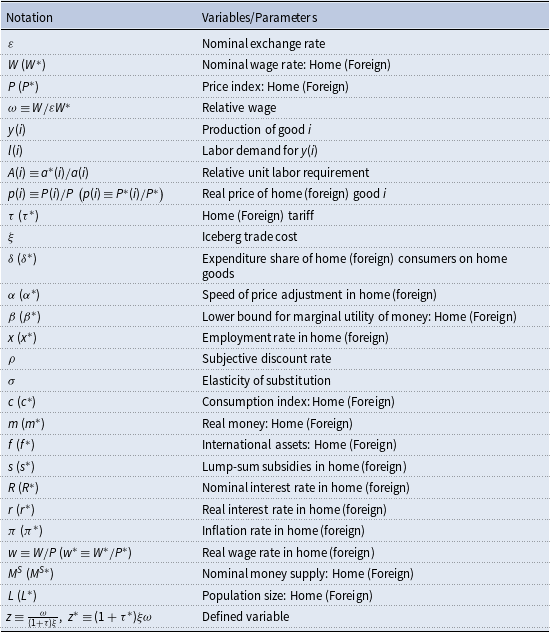
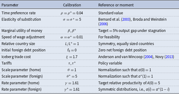

 τ(∗)
 ξ

 τ
 τ∗


