Introduction

The monitoring of small Antarctic glaciers is of interest because the glaciers are expected to be sensitive even to small environmental changes and could therefore provide clear evidence of current and recent climatic changes. The use of traditional methods to obtain the mass balance or to monitor the surface topography involves some problems that could affect the results. It is very difficult to maintain a network of slakes on a glacier surface; stakes may be broken by the wind, be buried in accumulation areas or melt out and fall in ablation areas. The number of measured slakes seldom equals the number initially positioned. These problems are enhanced in Antarctica since it is not possible to have a glaciological party in every year’s expedition.

The use of traditional surveying instruments like theodolites is also problematic in Antarctica. Surveys are restricted by weal her conditions, particularly by the wind. Moreover, traditional survey operations require good visibility between stations.

Global positioning system (GPS) surveying can overcome many of the obstacles to traditional methods. We used continuous kinematic GPS at several Antarctic locations to evaluate the technique for the study of surface variations on smaller glaciers.

Kinematic Gps In Antarctica

Kinematic GPS is a satellite-based survey method that allows the trajectory of a moving receiver to be computed. The relative position accuracy of a moving GPS receiver is related mainly to the quality of the signal reception, to the distance from a fixed reference station and to she satellite constellation available during the survey. Under normal conditions, at mid-latitudes, accuracy over distances of 10–15 km is on the order of a few centimetres (Landau, 1989).

Precision kinematic surveys require a minimum of two geodetic (phase-tracking) GPS receivers. The relative positions (at a few centimetres level of accuracy) with respect to the reference frame of fixed stations tan be available in near real-time mode (Bitelli and others, 1994), if the receivers are equipped with real-lime kinematic (RTK) firmware and hardware, or can be computed after the survey is complete. During an RTK survey the reference station acquires GPS signals and transmits code and phase observations to a roving receiver through a radio link. The rover receiver uses the firmware installed in the instrument to perform precise positioning (using GPS carrier phase measurements) in neat real time, but the final solution is usually computed using one frequency only. Post-processing permits more interaction with data and allows the full use of both GPS carrier frequencies (L1 and L2). Different linear combinations of the L1 and L2 signals permit, for example, mitigation of ionospheric noise or improvement in the ambiguities-resolution techniques. However, the solution is computed after the survey, so it is not possible to navigate along the planned routes with high accuracy.

In equatorial and auroral areas irregularities in the structure of the ionosphere cause a scintillation effect on the GPS signal acquisition. Such interference is particularly critical for high-accuracy GPS surveys because it creates cycle slips which make integer estimation of the phase ambiguities difficult. Using dual-frequency receivers could be useful in these conditions even for short baselines. Advanced

Fig. 1.

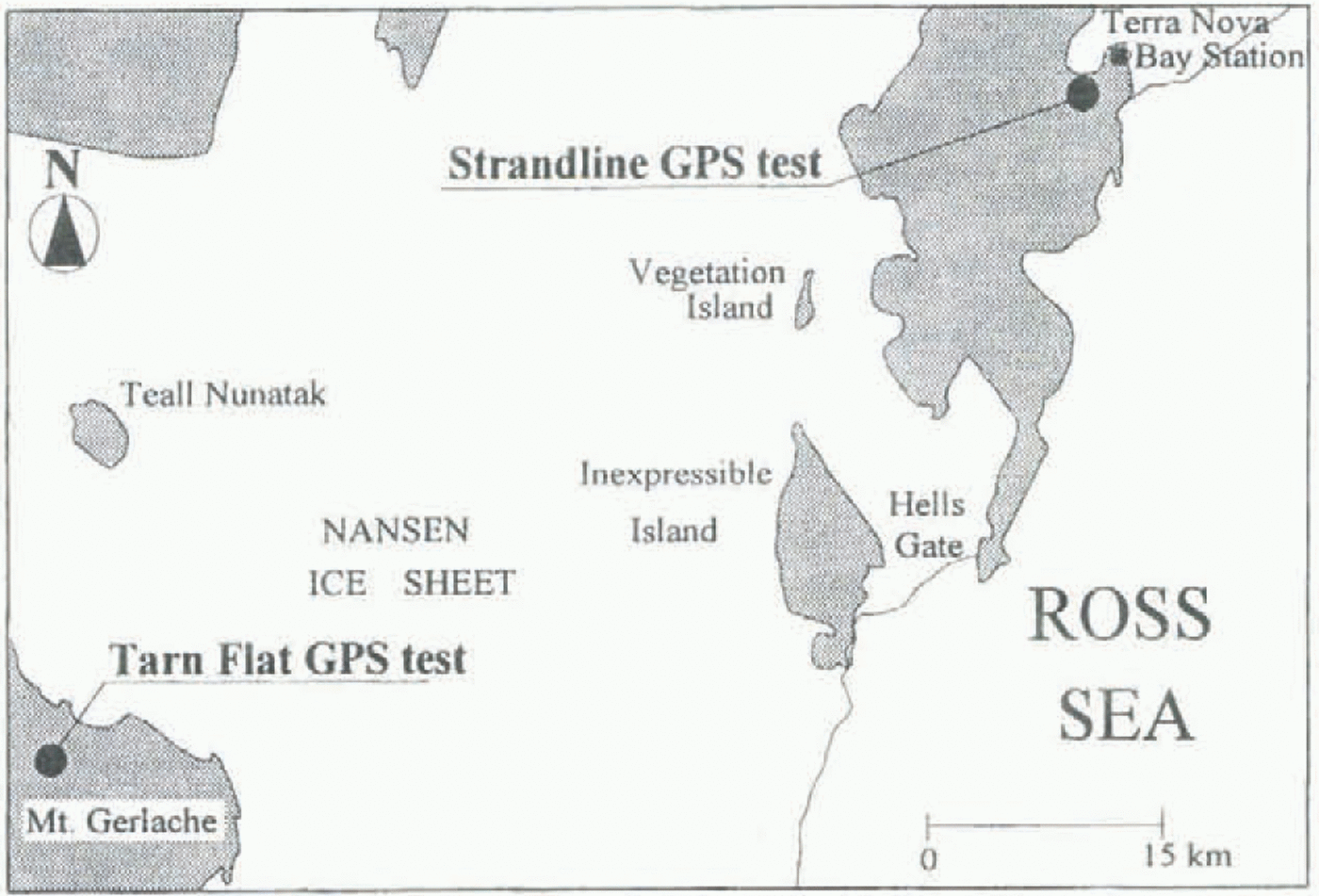
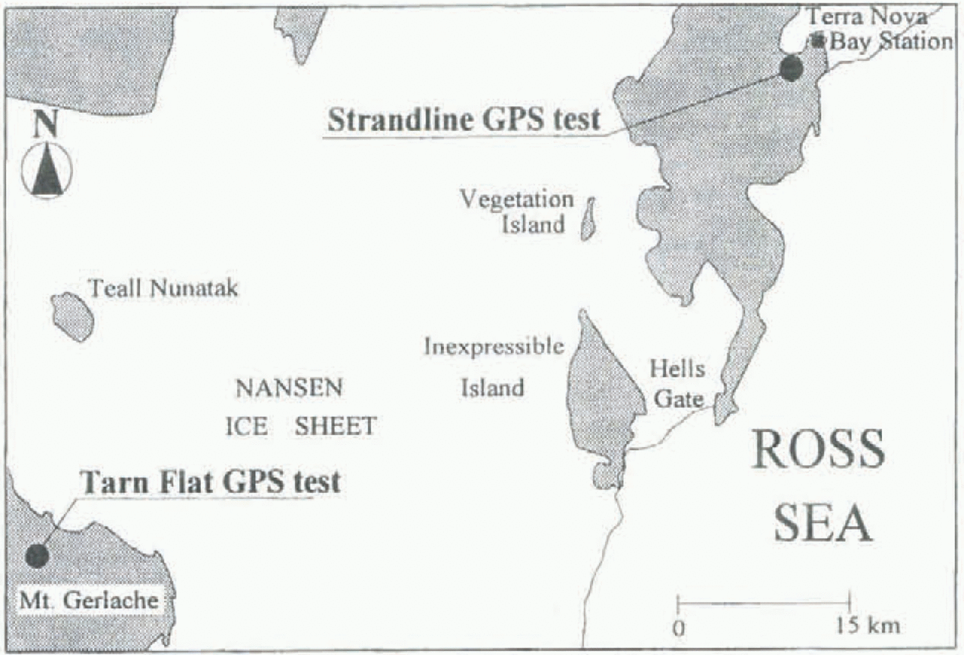
Location of field sites.

post-processing software complete with “On-The-Fly” (OTF) algorithms (Euler and Landau, 1992) can help resolve critical kinematic surveys. OTF techniques allow integer values of the initial phase biases to be fixed without a known initial position or static initialization. These techniques are particularly useful when GPS signals are interrupted (by large or rapid ionospheric disturbances, obstacles, etc.) during the survey.

Experimental Tests

The tests were conducted on two glaciers in the Terra Nova Bay area, Victoria Land, Antarctica. One is Strandline Glacier, so called by Chinn and others (1989); the other is an unnamed glacier located at Tarn Flat, east of Mount Gerlache (Fig. 1). Both glaciers are cold; their accumulation and ablation areas are controlled by wind and are irregularly distributed. The two glaciers have been investigated by Italian researchers since 1987 (see references in Baroni and others (1995)).

Fig. 2.

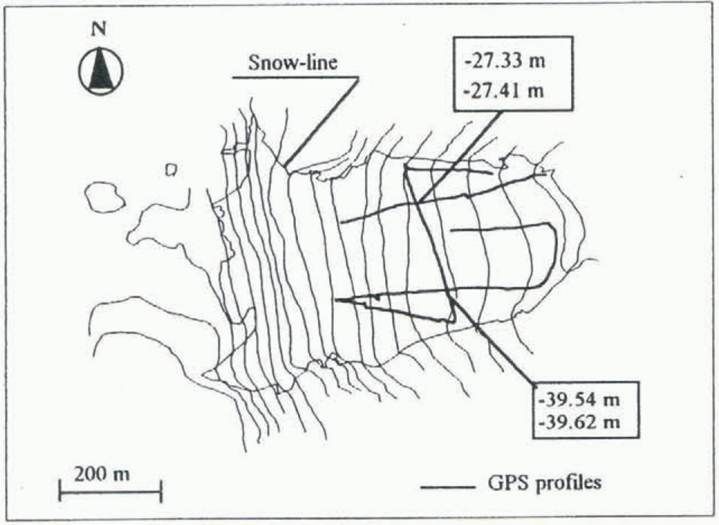
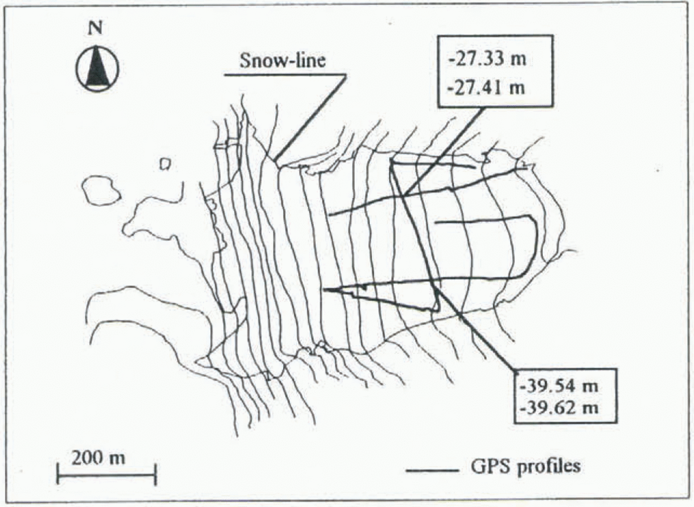
Profiles surveyed by GPS on Strandline Glacier. Elevations above sea level (mean geoidal undulation to WGS84 for the area −57.2 m, contour interval 20 m).

The GPS surveys started during the 1993 91 expedition and were repeated in full during the 1995–90 campaign. During the 1994–95 campaign a partial survey was carried out on Strandline Glacier.

Two sets of GPS antenna and receiver (Trimble 4000 SSEs) were used. For each survey, one of the instruments was set up on a benchmark fixed on a nearby bedrock. The reference points were linked to the Italian geodetic network in order to maintain a common reference system (WGS84)

Fig. 3.

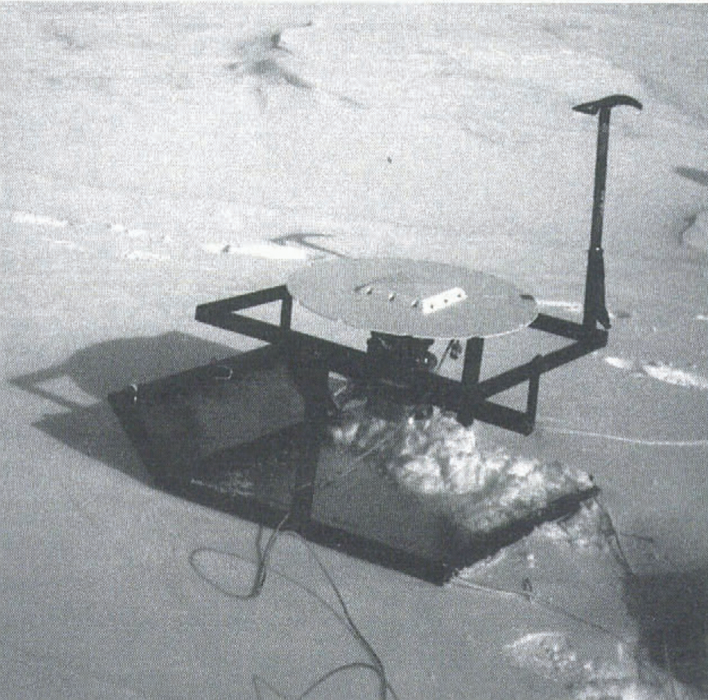
GPS sledge.

in successive campaigns. This fixed receiver was used as reference station, while the second (rover receiver) was carried along a survey path.

Validation (epoch by epoch) of a continuous kinematic GPS survey is possible using at least four receivers (two installed on a mobile object and two located at reference points). Two independent positions are computed (epoch by epoch), and the geometric relation between rover antennas can be used as a test.

In our experiment, however, only two GPS receivers were available. To provide an independent check on the survey, static or fast-static observations (20–45 min of dual-frequency data) were collected at the beginning and end of each surveyed profile or several profiles. This also provided the possibility for traditional kinematic survey initialization in those cases where the OTF initialization failed.

The antenna was fitted with a ground-plane to block signal reflections (multipath). The rover antenna was carried on a special sledge, which maintained the horizontal position of the antenna on steep slopes by a simple cardanic support. A counterbalance was fixed under the antenna to reduce swinging. The sledge was pulled along profiles while maintaining a phase lock with GPS satellites. Figure 2 shows the locations of the surveyed profiles mi Strandline Glacier. A photograph of the sledge is shown in Figure 3.

Data Processing And Comparison

GPS data were usually pre-analyzed to verify their quality and to identify problematic acquisition (i.e. periods affected by multipath or cycle slips). Pre-analysis was done using the Quality Control software of UNAVGO (University Navstar Consortium). The “GPS-Edit” developed by TerraSat (Munich), was used for graphical interaction on problematic acquisitions before and during the processing phase (i.e. elimination of the small part of single satellite acquisition affected by multipath. high noise, etc.). The 1993–94 Strandline Glacier survey required extensive manual interaction to eliminate data affected by high noise.

We then verified that differences between kinematic positions and the static cheek points computed separately

Fig. 4.

Height values at profile intersections during the 1993–94 Strandline survey (WGS84 heights).

were less than 0.1 m. Next, static and kinematic measurements were merged and the rover-receiver trajectory was computed using the Geotracer GPS software developed by TerraSat (Munich). Considering the short distances between rover and fixed receiver (<5 km) a fixed solution on both the L1 and L2 frequencies was easily reached using the OTF algorithm.

OTF algorithms, designed mainly for airborne GPS, are also useful for land kinematic GPS applications because

Fig. 5.

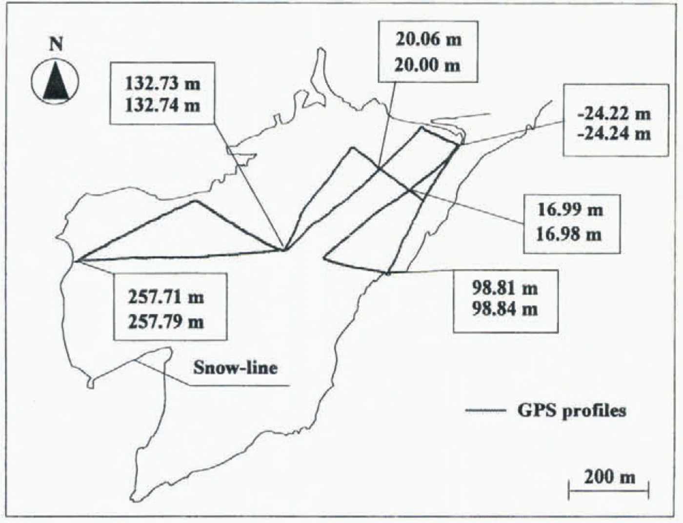
Height values at profile intersections during the 1993–94 Tarn Flat survey (WGS84 heights). GPS profiles are reported on a photogrammetrically derived contour map (1956 flight, contour interval 20 m).

they can tolerate the frequent cycle slips induced by the ionosphere (Vittuari, 1994). Ionospheric interference in auroral areas degrades the signal-to-noise ratio and causes erroneous phase-cycle count, and cycle slips that may occur without apparent loss of lock (Viterbi, 1966; Ciraolo, 1994).

The OTF algorithm included in the Geotracer program consists of the following steps.

A preliminary solution using the code modulated on the GPS frequencies is scanned to locate an optimal observation time-span for ambiguity resolution. The number of satellites in view, time-span of continuous observation, and satellite-geometry (position dilution of precision; PDOP) value are checked. OTF ambiguity resolution is performed on each selected interval using the following procedure:

1. (1) A solution using float carrier phase ambiguities for each satellite is estimated.

2. (2) Estimated ambiguities are used to find a fixed solution.

3. (3) The sets of ambiguities are validated statistically to guarantee the desired (centimetre-level) accuracy.

4. (4) Validated ambiguities are fixed and propagated through the whole tracking time between losses of lock for each satellite.

The post-processing software estimates error due to satellite constellation geometry (geometric dilution of precision; GDOP). The value of GDOP computed epoch-by-epoch for the different surveys did not exceed 6 (usually GDOP <7 is acceptable), and only a few epochs, recorded immediately after a loss of lock and rejected during the subsequent analysis, had/ GDOP values as high as 10.

The repeatability of the method can be estimated from crossover errors. The examples of GPS profile crossovers for Strandline Glacier and Tarn Flat are shown in figures 4 and 5, respectively. The maximum difference in GPS-determined elevation shown in the figures is 0.08 m, and the same level of repeatability was obtained for the other surveys.

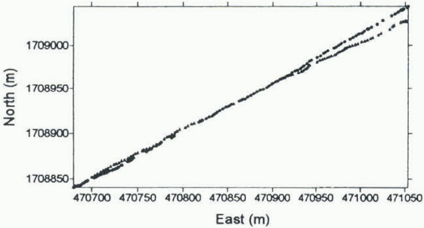
GPS-survey paths from different years differ slightly. This is because all the surveys were made without the instrumental capabilities to solve for the precise position in real-time mode. Natural reference points available on and around glaciers were used instead. Survey path separation is usually a few metres. Thus, direct comparison between homologous profiles is not possible. The problem is greatest where there is a large vertical gradient across the profiles.

Two different methods of inter-survey comparison are tested.

Method 1

For the first comparison, a narrow strip of digital terrain model (DTM) is constructed (1 m grid using a linear kriging method for interpolation) along each profile. All the points available in the area for the same survey are used. Next the planimetric line which best approximates each group of homologous traces is determined. The relative altimetric track of each surface through the planimetric line is computed (with a step of 5 m), in order to build coincident

Fig. 6.

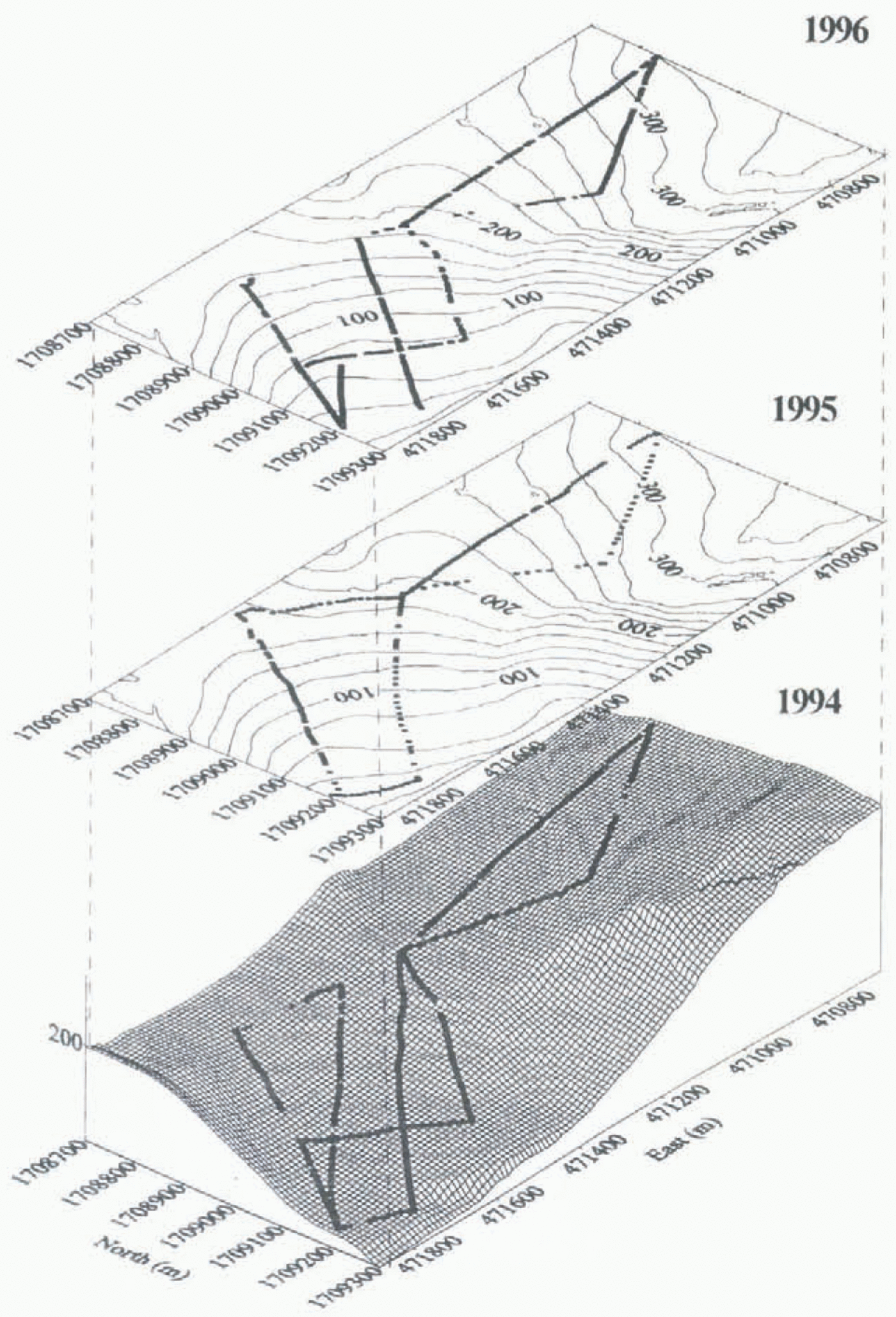
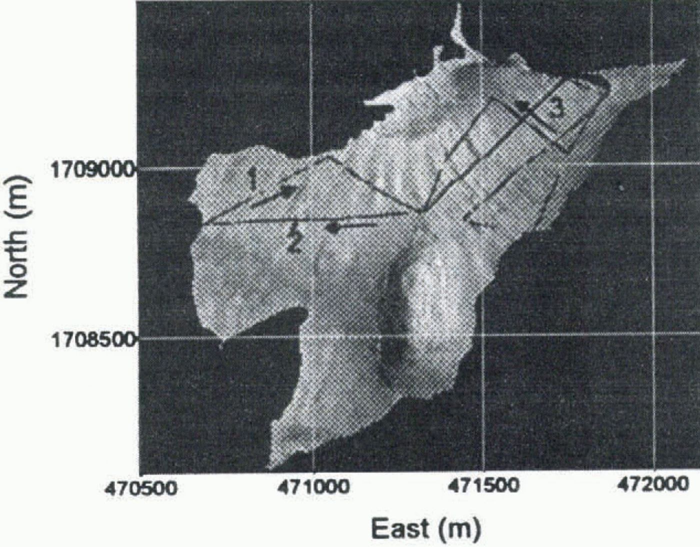
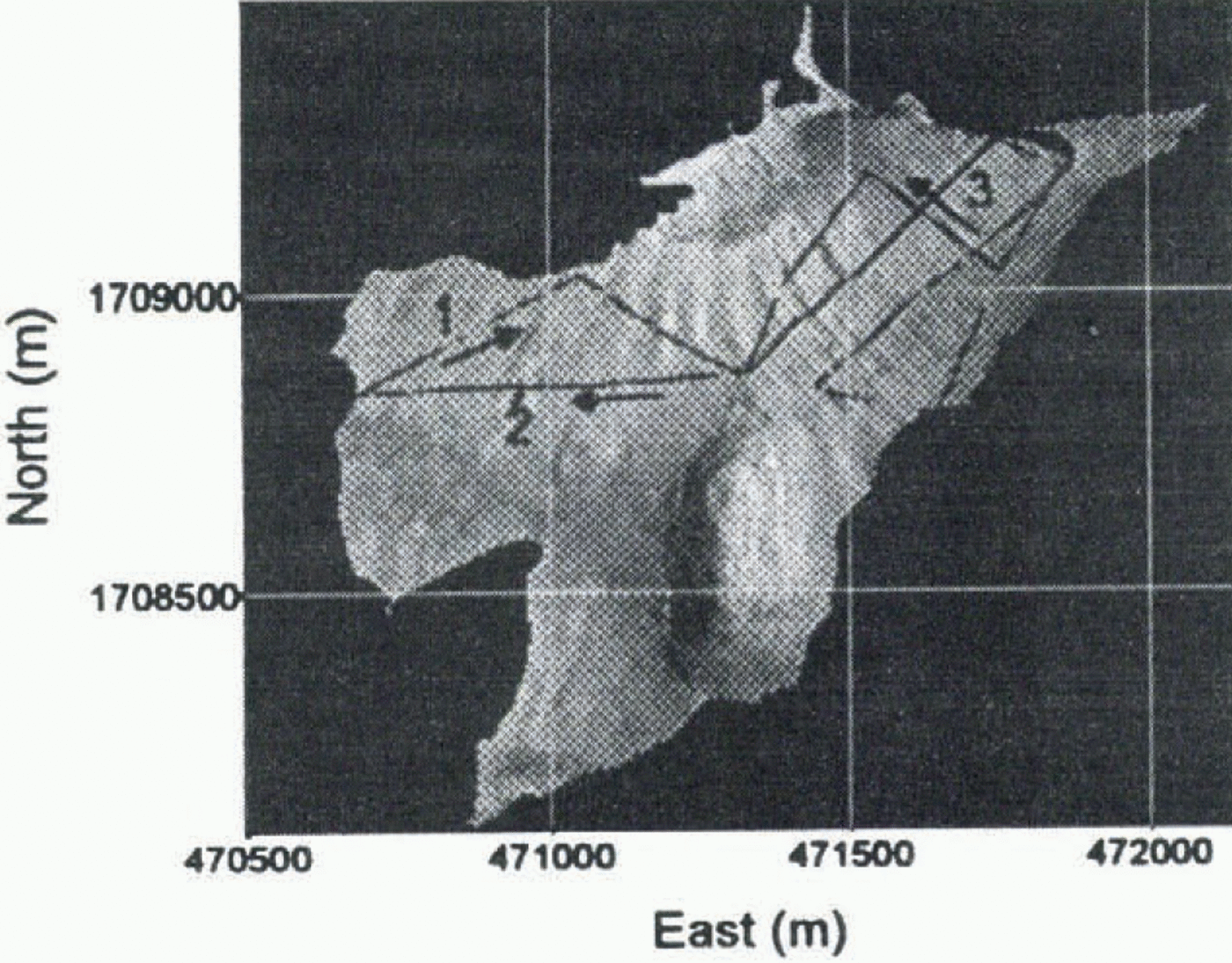
Kinematic GPS routes on Strandline Glacier, plotted on a photogrammetrically derived DTM (UTM–WGS84 coordinates).

Fig. 7.

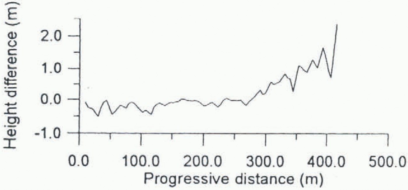
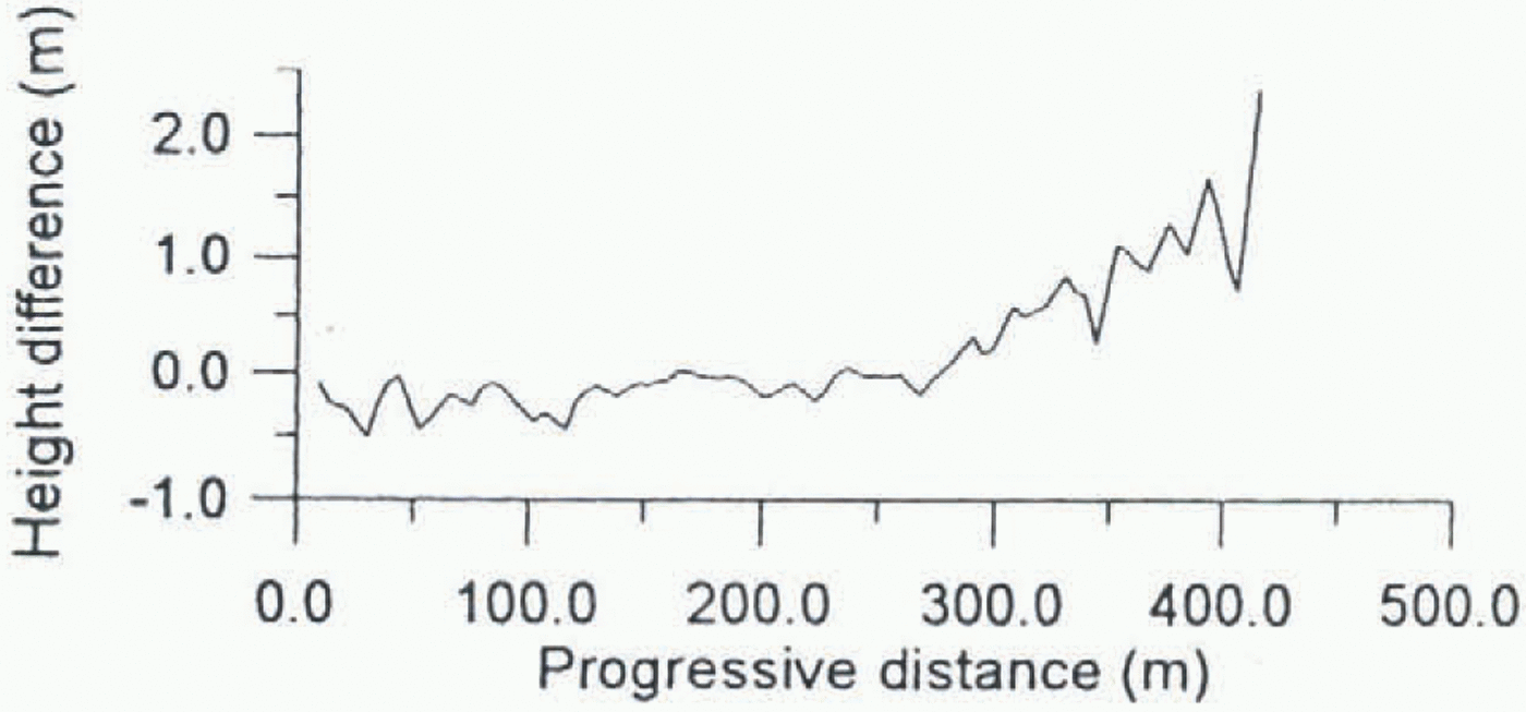
Difference between the 1993–94 and 1995–96 surveys of Strandline Glacier profile 1, computed using the first method (progressive distance is computed from the origin of profile).

Fig. 8.

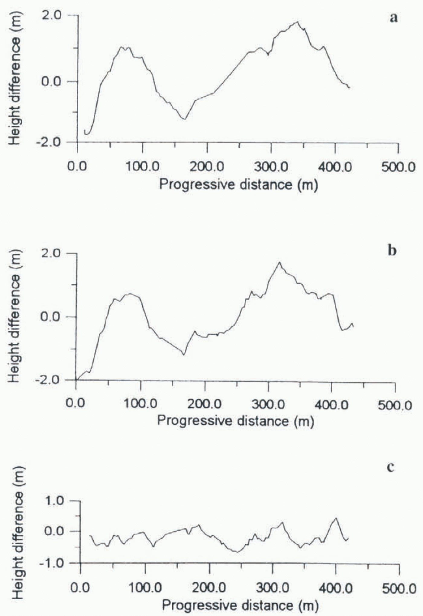
Comparison of profile 1 (progressive distance is computed along the lines that fit profiles). (a) Difference between 1993–94 survey and photogrammetrically derived DTM. (b) Difference between 1995–96 survey and photogrammetrically derived DTM. (c) Difference between curses in (a) and (b).

profiles. In this way comparison may be made on the same planimetric trace.

Method 2

The second approach compares the profiles and a known DTM of the glacier. This is possible on Strandline Glacier, for which a 1985 photo strip is available and a numeric contour map (scale 1:10 000) was obtained by analytical plotting. External orientation of stereo pair is carried out using ground-control points surveyed by static GPS observations made during the 1993–94 campaign. Residuals for the external orientation are at the 1 m level (Baroni and others, 1995).

Starting in the 1993–94 campaign, the geodetic reference system used for all surveys at Terra Nova Bay Station was the International Terrestrial Reference Frame (ITRF). The ITRF was established for the Terra Nova Bay geodetic network through a global adjustment carried out within the framework of international GPS campaigns. This reference system is used for both the photogrammetric ground-control points survey and the reference stations used during kinematic surveys. WGS84 and ITRF can be considered to be equivalent for the purposes of this work.

A DTM with a 5 m grid was computed from the contour map using a linear kriging method for the interpolation. Comparisons between several homologous profiles using the two methods described above are reported here. Planimetric tracks of the considered profiles plotted on the Strandline Glacier DTM are shown in Figure 6.

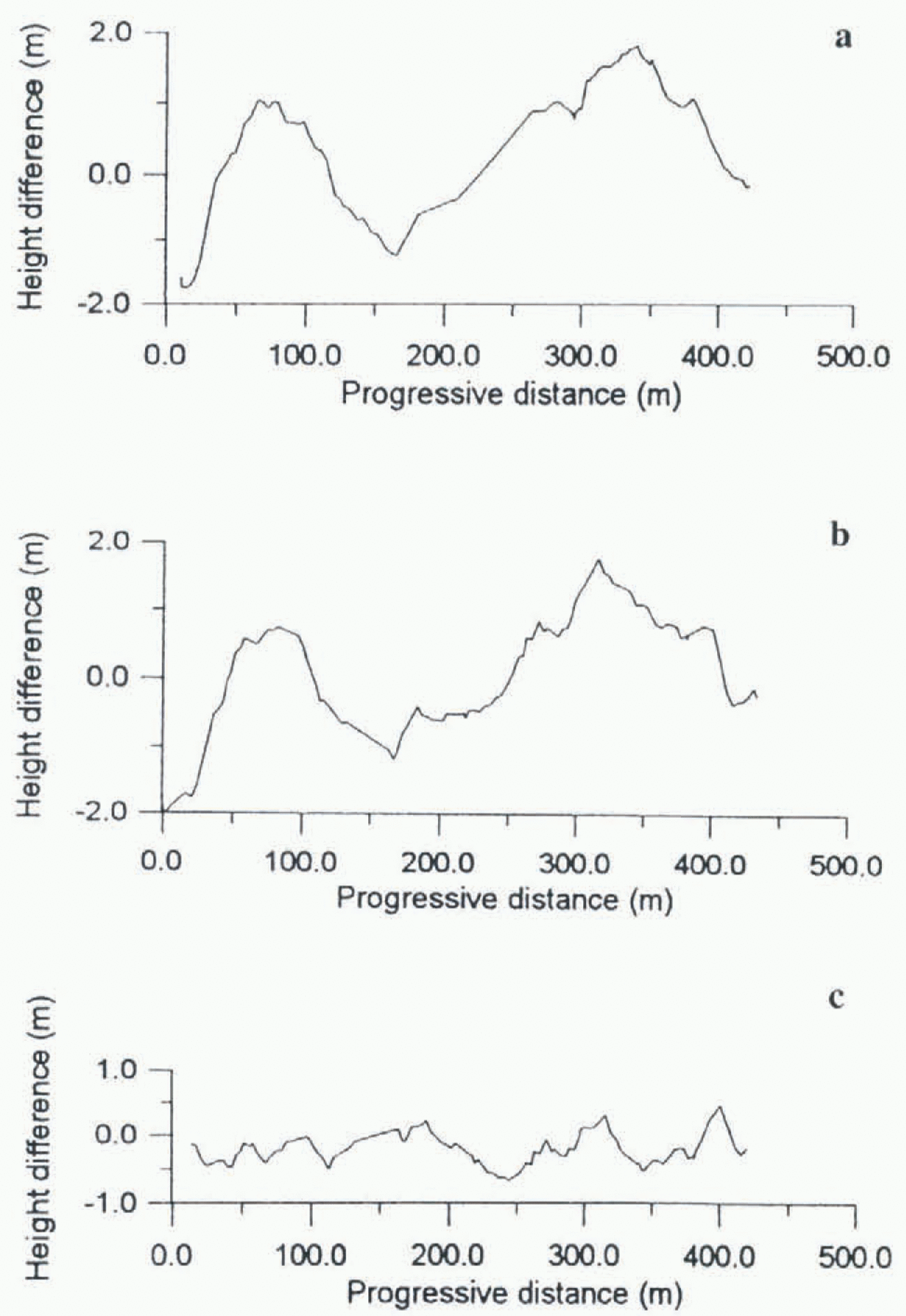
Differences between 1993–94 and 1995–96 elevations along profiles 1, 2 and 3 (Fig. 6) are used to evaluate the two comparison methods. Results for method 1 are shown in Figure 7. For the second comparison method, each year’s

Fig. 9.

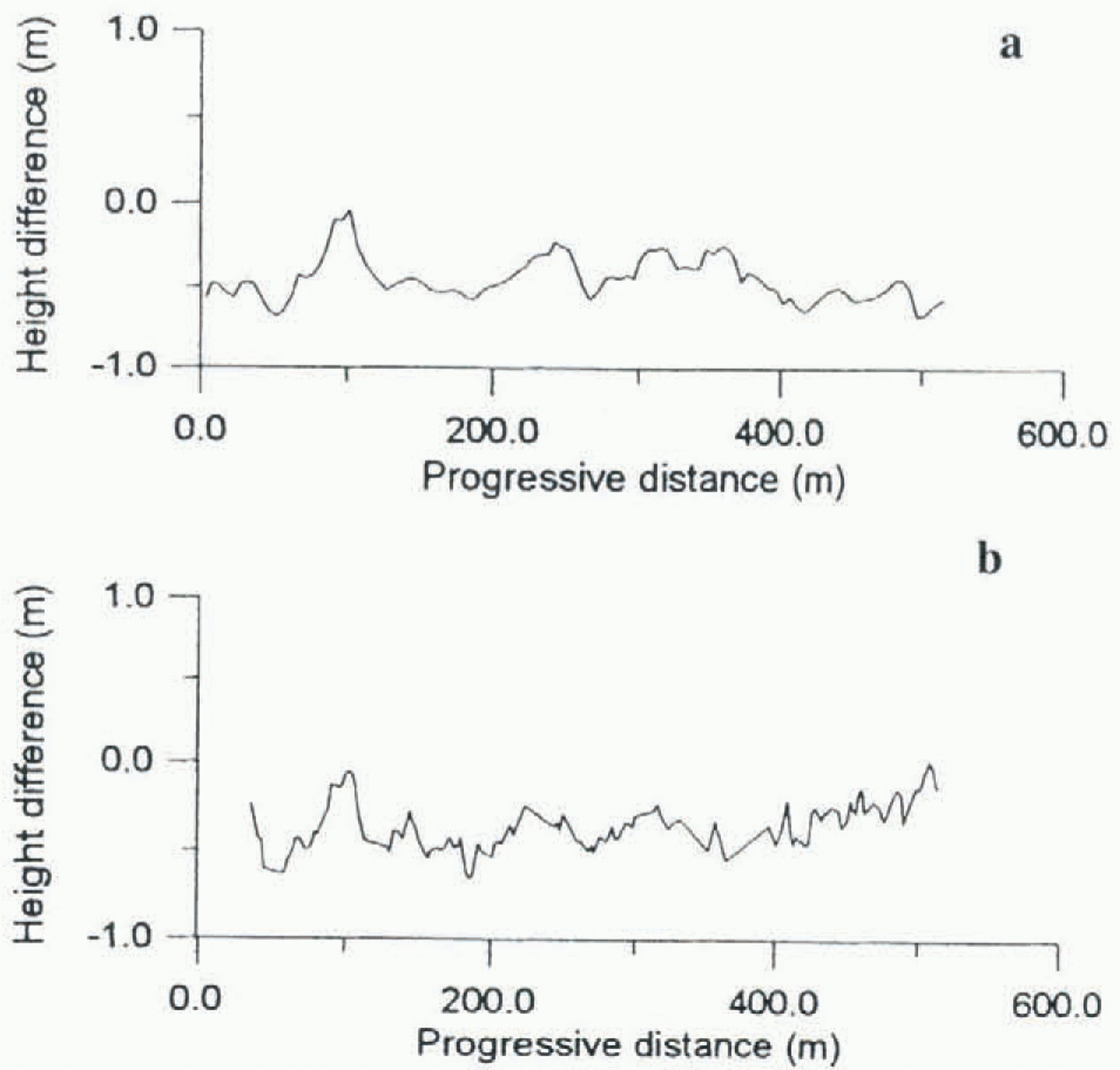
Comparison of profile 2 relative to the determinations of 1993–94 and 1995–96: (a) differences using first approach, (b) differences using the comparison with the known DTM.

Fig. 10.

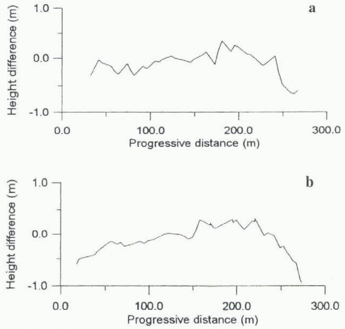
0Comparison of profile 3 relative to the determinations of 1993–94 and 1995–96: (a) differences using first approach, (b) differences using the comparison with the known DTM.

Fig. 11.

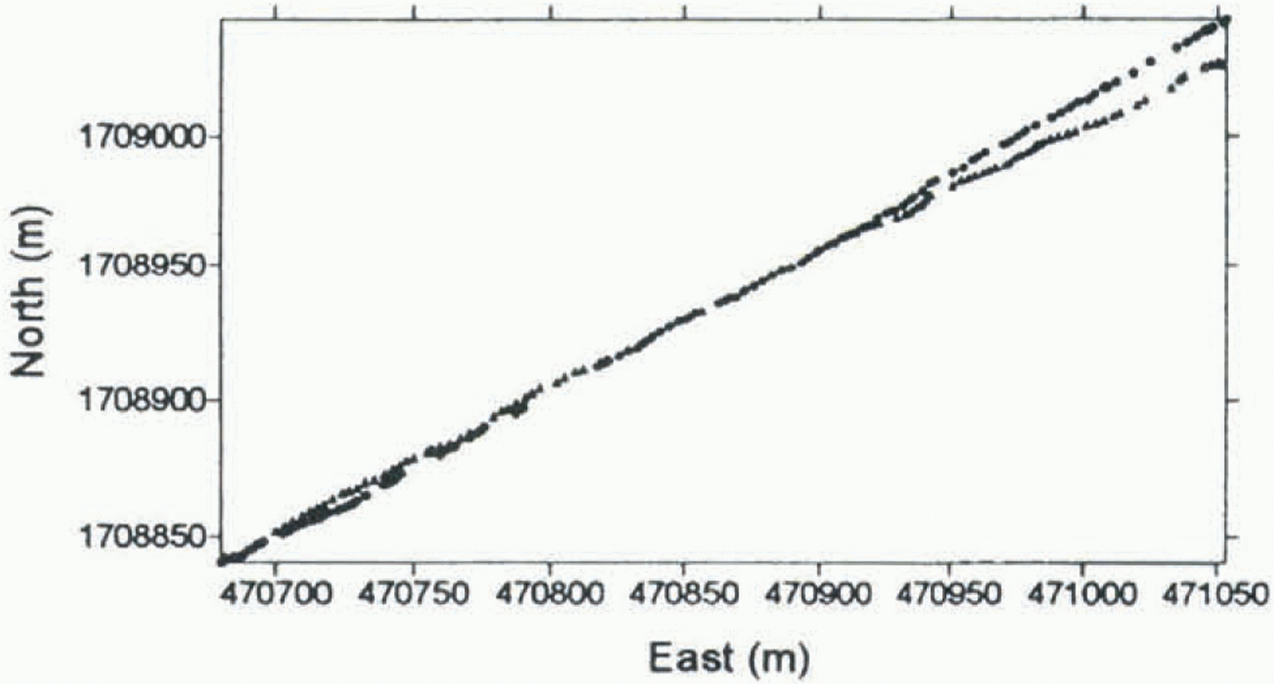
Planimetric displacement between 1993–94 and 1995–96 surveys for profile 1.

GPS survey is compared with the 1985 DTM. Differences between the 1993–94 survey of profile 1 and the DTM and between the 1995–96 survey of profile 1 and the DTM are shown in figure 8a and b, respectively. The difference between the curves in figure 8b and a is shown in figure 8c (progressive distance is computed from the starting-point of the profile).

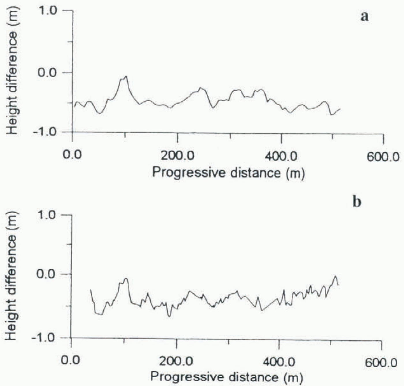
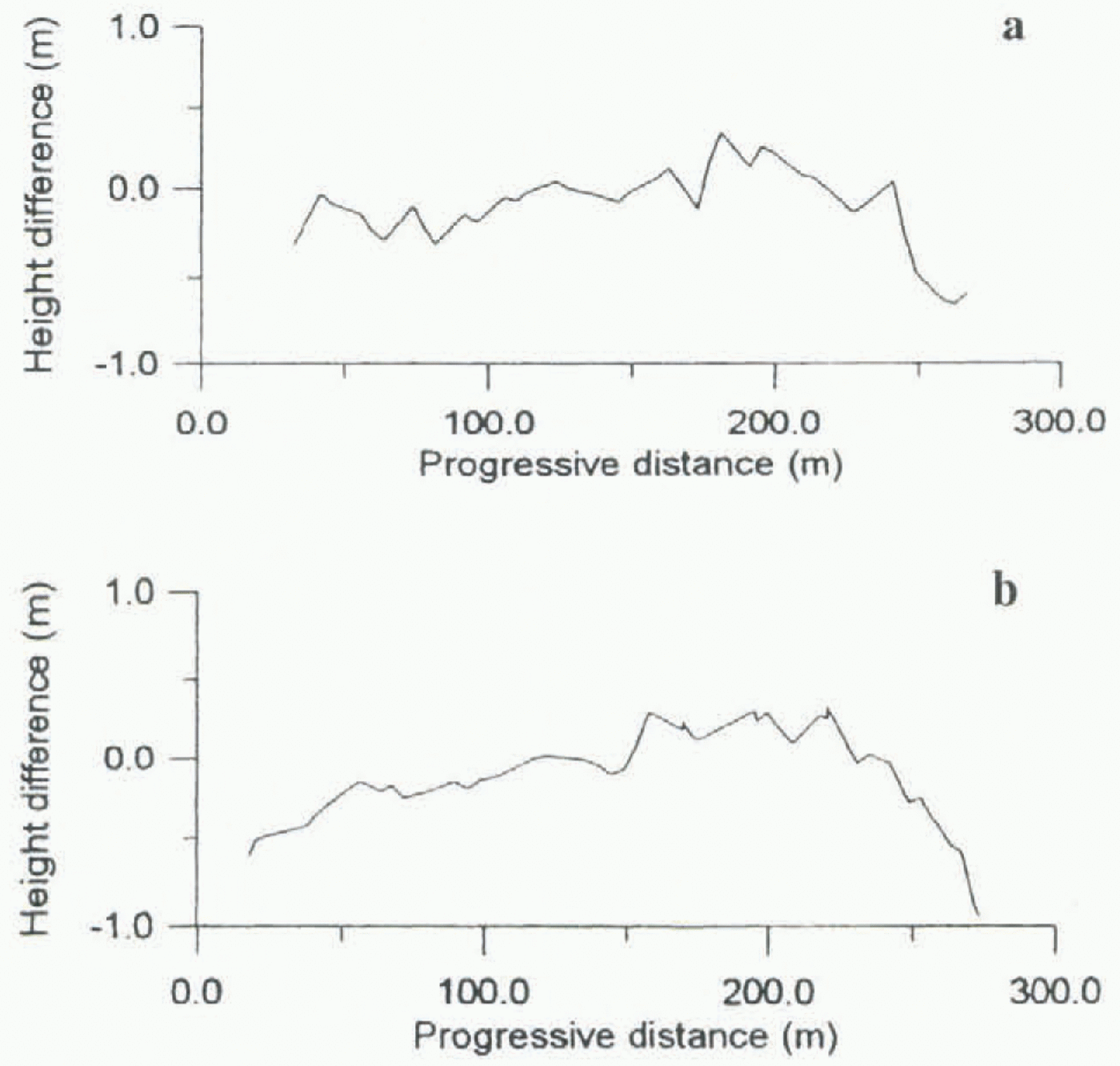
Results of the two methods for profiles 2 and 3 are shown in figures 9 and 10, respectively.

Both methods correct for horizontal displacement of GPS-survey tracks in different years: the first by interpolation of a common profile, the second by consideration of the displacement from a known surface between profiles. The first approach gives reliable results when the surveyed points are evenly distributed. The second approach supplies the variation of the surface with respect to the known DTM. Method 2 may only detect changes when the variation of the surface between successive surveys can be considered homogeneous across the profile for the narrow strip of profile displacement.

Different factors determine the accuracy of the two methods. Method 1 is sensitive to the spatial distribution of surveyed points. This is demonstrated by the difference between the curves in figures 7 and 8c over the interval 350–425 m. Kriging can be used to perform either exact or smoothed interpolation. If the surveyed points are homogeneously distributed and exact interpolation is used, the accuracy of DTM should be at the same level as the original

Table. 1

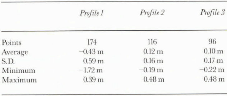
Table 1. Statistics of differences between the curves obtained using method 1 and method 2 for comparison of profiles

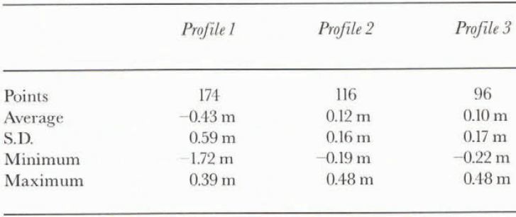
points. The interpolation is poorly constrained at the edge of the DTM. The sensitivity of the first comparison method to edge effects is evident where the planimetric displacement is large (Fig. 11). The second comparison method’s optimal accuracy is equal to that of the known DTM but is degraded by spatial displacement between different years’ surveys. To quantify the errors invoked for the whole process of interpolation a direct comparison is made between the sets of two curves (methods 1 and 2). The results are shown in Table 1. When the displacement between profiles is within a few metres and across-track slopes are small (5–15°) the results of the two methods have standard deviations less than 20 cm (profiles 2 and 3). Both methods partially compensate for the spatial displacement of profiles. (For a 5 m displacement and an across-track slope of 15° the unconnected elevation difference would be 1.3 m.) Where the displacement was large (on the order of 20 m at the end of profile 1) the comparison became useless. It is not possible to attribute the error to the first comparison method because, wish 20 m displacement between profiles, the accuracy of the second method is the same as the accuracy of the original known DTM (± 1 m).

Conclusion

Sledged-GPS surveying provided reliable results in the experiments presented here (in terms of repeatability). The main limitation is spatial displacement between profiles in successive years. Errors due to displacement were reduced by careful interpolation, but the accuracy degraded to the 20 cm level. The problem can be partially avoided using a homogeneous distribution of profiles on the investigated surface or using an accurate known DTM as a reference.

Real-time kinematic positioning would allow profiles to be repeated exactly, avoiding displacement errors entirely. Moreover, this method would open new strategies of GPS monitoring of glaciers, for example, the repetition of measurements on a regular grid of control points.