1 Introduction
Antarctic ice shelves melt by turbulent transport of heat and salt to the ice face, predominantly under the influence of warmer and salty Circumpolar Deep Water entering ice shelf cavities from the surrounding Southern Ocean (Payne et al. Reference Payne, Vieli, Shepherd, Wingham and Rignot2004; Rignot et al. Reference Rignot, Bamber, Van Den Broeke, Davis, Li, Van De Berg and Van Meijgaard2008). The water exiting ice shelf cavities contributes to Antarctic Bottom Water, which in turn is a crucial component of the global thermohaline circulation. Both heat and salinity play a significant role in the melting process which takes place inside a boundary layer on the ice face. Knowledge of the boundary layer, the factors governing melting of the ice, and the feedbacks between them, is needed to predict melting rate and future rises in sea level.
Recent field measurements by Jenkins et al. (Reference Jenkins, Dutrieux, Jacobs, Mcphail, Perrett, Webb and White2010) near Pine Island Glacier used an autonomous underwater vehicle to provide detailed measurements of the water column close to the melting ice sheet. However, the flow field near the ice–water interface is very difficult to measure in the field, and the only observations available come from laboratory experiments on melting of ice under oceanic conditions. For a block of ice with vertical sides in room temperature water with a vertical salinity gradient, experiments show the formation of double-diffusive layers and the efficient mixing of melt water with the surrounding salty water (Huppert & Turner Reference Huppert and Turner1978, Reference Huppert and Turner1980; Huppert & Josberger Reference Huppert and Josberger1980). Other experiments have examined the rate of melting and boundary layer flow at a vertical ice of
 $O(1)$
m high in water at a range of (uniform) far-field temperatures and a salinity (35 ‰) near that of seawater (Josberger & Martin Reference Josberger and Martin1981) or for varying ambient water temperatures between
 $1\,^{\circ }\text{C}$
and
 $15\,^{\circ }\text{C}$
with a relatively low salinity (10 ‰) (Carey & Gebhart Reference Carey and Gebhart1982). When focusing on Antarctic conditions, seawater temperatures are close to
 $0\,^{\circ }\text{C}$
(e.g. Rignot & Jacobs Reference Rignot and Jacobs2002; Payne et al.
Reference Payne, Vieli, Shepherd, Wingham and Rignot2004). At these low temperatures, the change of phase from solid ice to liquid is governed primarily by transfer of solute to the ice–water interface and so is more accurately referred to as dissolution (Woods Reference Woods1992; Kerr Reference Kerr1994a
,Reference Kerr
b
; Wells & Worster Reference Wells and Worster2011). Melting, on the other hand, is governed by heat transfer and occurs in warmer water. Recent laboratory experiments by Kerr & McConnochie (Reference Kerr and Mcconnochie2015) with ice dissolution, again at a 1.2 m scale, gave results that compare well with a new theoretical model they developed for dissolution by turbulent compositional convection. The theory predicts that the dissolution velocity depends on the
 $4/3$
power of the difference between the ocean temperature and its freezing point.
The ice–ocean interaction problem is computationally challenging because the grid size must be sufficiently small that both the thermal and salinity boundary layers are resolved. The salinity boundary layer width
 ${\it\delta}_{s}$
is of the order of 0.1 mm, an order of magnitude smaller than the thermal boundary width
 ${\it\delta}_{H}$
(Kerr & McConnochie Reference Kerr and Mcconnochie2015). At the micro-level the role of the diffusion of salt to the ice–ocean interface, which governs dissolution of the ice, is of key importance (Wells & Worster Reference Wells and Worster2011; Kerr & McConnochie Reference Kerr and Mcconnochie2015). Global ocean models (Holland & Jenkins Reference Holland and Jenkins1999; Holland, Jenkins & Holland Reference Holland, Jenkins and Holland2008) and regional ocean modelling systems (Galton-Fenzi et al.
Reference Galton-Fenzi, Hunter, Coleman, Marsland and Warner2012) resolve the flow field at only much larger scales (
 ${>}O(1)$
km) and rely on parameterizations of the smaller unresolved scales, including the boundary layer against the ice interface. In this first report on direct numerical simulation (DNS) of the turbulent convection and the dissolution we address the problem of a vertical ice face in contact with a uniform ocean in which we assume no motion apart from the convection produced by the ice–ocean contact. We also restrict our simulations to scales used in the previous laboratory experiments, partly for a direct comparison and partly owing to computational demands of larger scales, and show that these can be fully resolved by DNS. The simulations provide the first spatial and temporal information on the turbulent convection. They are used to test previous theoretical and experimental results and to examine the energy input to turbulence, preparing the way to modelling of geophysical conditions.
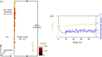
(a) Schematic of the domain used for the simulation: the vertical ice face of height
 $H$
is placed at the left-hand side of the domain and ice is in contact with seawater at initial temperature
 $T_{w}$
and salinity
 $S_{w}$
. The right-hand side of the domain has an open boundary condition by using a sponge layer (Klemp & Durran Reference Klemp and Durran1983). Interface conditions (
 $T_{i},S_{i}$
and dissolution velocity
 $V$
) are evaluated from heat and salinity flux balance at that surface. Superposed is a snapshot of the temperature field
 $T$
in the
 $x$
–
 $z$
plane in a thermally equilibrated numerical simulation. (b) Evolution of the interface temperature and dissolution velocity with time at the mid-depth of the vertical ice face for a far-field temperature
 $T_{w}=2.3\,^{\circ }\text{C}$
and salinity
 $S_{w}=35$
‰.

2 Formulation of the problem and solution techniques
2.1 Problem set-up
The flow field is solved using DNS in a tall rectangular domain with length
 $L$
(normal to the ice interface), width
 $W$
(along the ice interface, in which direction the domain is periodic) and height
 $H$
, as shown in figure 1(a). The saline water has kinematic viscosity
 ${\it\nu}$
, thermal diffusivity
 ${\it\kappa}_{T}$
, salinity diffusivity
 ${\it\kappa}_{S}$
, coefficient of thermal expansion
 ${\it\alpha}$
and coefficient of haline contraction
 ${\it\beta}$
. As the flow involves only a small range of temperature, the real equation of state is closely approximated as linear. Navier–Stokes equations under the Boussinesq approximation are written in Cartesian coordinates [
 $x,y,z$
] and in dimensional form as
 $$\begin{eqnarray}\displaystyle & \displaystyle \boldsymbol{{\rm\nabla}}\boldsymbol{\cdot }\boldsymbol{u}=0, & \displaystyle\end{eqnarray}$$
 $$\begin{eqnarray}\displaystyle & \displaystyle \frac{\text{D}\boldsymbol{u}}{\text{D}t}=-\frac{1}{{\it\rho}_{0}}\boldsymbol{{\rm\nabla}}p^{\ast }+{\it\nu}{\rm\nabla}^{2}\boldsymbol{u}-\frac{{\it\rho}^{\ast }}{{\it\rho}_{0}}g\boldsymbol{k}, & \displaystyle\end{eqnarray}$$
 $$\begin{eqnarray}\displaystyle & \displaystyle \frac{\text{D}T^{\ast }}{\text{D}t}={\it\kappa}_{T}{\rm\nabla}^{2}T^{\ast }, & \displaystyle\end{eqnarray}$$
 $$\begin{eqnarray}\displaystyle & \displaystyle \frac{\text{D}S^{\ast }}{\text{D}t}={\it\kappa}_{S}{\rm\nabla}^{2}S^{\ast }, & \displaystyle\end{eqnarray}$$
 $$\begin{eqnarray}\displaystyle & \displaystyle {\it\rho}^{\ast }={\it\rho}_{0}({\it\beta}S^{\ast }-{\it\alpha}T^{\ast }). & \displaystyle\end{eqnarray}$$
 $\boldsymbol{u}=(u,v,w)$
is the flow velocity,
 ${\it\rho}_{0}$
is fixed reference density and
 $p^{\ast }$
,
 $T^{\ast }$
,
 $S^{\ast }$
and
 ${\it\rho}^{\ast }$
denote deviation from the background hydrostatic pressure
 $p_{b}$
and far-field temperature
 $T_{w}$
, salinity
 $S_{w}$
and density
 ${\it\rho}_{w}$
(e.g.
 $S^{\ast }=S-S_{w}$
). Governing parameters are the Grashof, Prandtl, Schmidt and Stefan numbers, and the buoyancy ratio,
 $$\begin{eqnarray}Gr=\frac{{\it\beta}g(S_{w}-S_{i})H^{3}}{{\it\nu}^{2}},\quad Pr=\frac{{\it\nu}}{{\it\kappa}_{T}},\quad Sc=\frac{{\it\nu}}{{\it\kappa}_{S}},\quad Sf=\frac{{\it\rho}_{s}L_{s}}{{\it\rho}_{w}c_{w}(T_{w}-T_{i})},\quad R_{{\it\rho}}=\frac{{\it\beta}(S_{w}-S_{i})}{{\it\alpha}(T_{w}-T_{i})}\end{eqnarray}$$
respectively, where
 $S_{i}$
and
 $T_{i}$
are salinity and temperature at the interface,
 ${\it\rho}_{s}$
and
 $L_{s}$
are the density and latent heat of the solid and
 $c_{w}$
is the specific heat of the saline water.
Conservation of heat and salt at the interface (
 $x=0$
) plays a key role in determining the dissolution velocity (e.g. Josberger & Martin Reference Josberger and Martin1981; Woods Reference Woods1992; Kerr Reference Kerr1994b
; Holland & Jenkins Reference Holland and Jenkins1999; Wells & Worster Reference Wells and Worster2011; Kerr & McConnochie Reference Kerr and Mcconnochie2015). The interface temperature
 $T_{i}=a_{S}S_{i}$
is controlled by
 $S_{i}$
, where the slope of the liquidus is
 $a_{s}=-6\times 1{0^{-2}\,}^{\circ }\text{C}/$
‰ and we have neglected the pressure dependent of liquidus over 1 m depth scale of the domain. Conservation of heat deals with the balance between latent heat due to dissolution
 $Q_{m}$
and the divergence of heat flux (
 $Q_{i}^{H}-Q_{w}^{H}$
) at the interface as
 $$\begin{eqnarray}Q_{i}^{H}-Q_{w}^{H}=Q_{m},\end{eqnarray}$$
where
 $Q_{i}^{H}={\it\rho}_{s}c_{s}{\it\kappa}_{T}^{S}\partial T/\partial x$
and
 $Q_{w}^{H}={\it\rho}_{w}c_{w}{\it\kappa}_{T}\partial T/\partial x$
are heat fluxes at the interface in the ice and water, respectively, and
 $Q_{m}={\it\rho}_{s}L_{s}V$
is the heat released during ice related to the ablation velocity
 $V$
. Here
 $c_{s}$
and
 ${\it\kappa}_{T}^{s}$
is the specific heat and molecular thermal conductivity of ice. To simplify the numerical formulation we ignore the conduction within the ice (
 $Q_{i}^{H}=0$
); the effect of this conductive heat transfer in the dissolution dynamics is described in Kerr & McConnochie (Reference Kerr and Mcconnochie2015) and is negligible for ice temperatures within several degrees of the interface temperature. The heat balance at the interface is then
 $$\begin{eqnarray}{\it\rho}_{s}L_{s}V=-{\it\rho}_{w}c_{w}{\it\kappa}_{T}\partial T/\partial x.\end{eqnarray}$$
Similarly, a flux balance condition between the fresh water release associated with melting,
 $Q_{s}$
(brine rejection), and the salt flux divergence (
 $Q_{i}^{S}-Q_{w}^{S}$
) at the interface gives
 $$\begin{eqnarray}Q_{i}^{S}-Q_{w}^{S}=Q_{s}.\end{eqnarray}$$
Based on ocean observations (Oerter et al.
Reference Oerter, Kipfstuhl, Determann, Miller, Wagenbach, Minikin and Graf1992) the diffusive salinity flux,
 $Q_{i}^{S}$
, in the ice and the salinity in the ice are negligible. The salt balance at the interface is then
 $$\begin{eqnarray}{\it\rho}_{s}S_{i}V=-{\it\rho}_{w}{\it\kappa}_{S}\partial S/\partial x.\end{eqnarray}$$
The latter condition maintains the interface salinity at
 $S_{i}$
. We impose horizontal velocity
 $u=-{\it\rho}_{s}/{\it\rho}_{w}V$
and
 $w=0$
at right-hand side of the fluid domain. The ice–water interface is assumed to remain planar and is fixed at
 $x=0$
. This assumption is based on a large Stefan number (
 $Sf\gg 1$
) and is supported both by a stable, planar interface observed in laboratory experiments (Kerr & McConnochie Reference Kerr and Mcconnochie2015) and the uniform ablation rate calculated here for the turbulent regime. In any case the assumption is valid over the short duration required for the present solutions. However, we caution that the interface morphology might potentially change with time if there are positive feedbacks between the interface shape, the flow and the ablation rate.
The right-hand side boundary of the computational domain is maintained as an open boundary by relaxing temperature and salinity on the boundary back to its background temperature
 $T_{b}$
and salinity
 $S_{b}$
, respectively (in a ‘sponge’ region
 $x=0.3~\text{m}$
to
 $x=0.5~\text{m}$
). At top and bottom boundaries a no-slip condition is imposed for velocities and a no-flux condition is maintained for the temperature and salinity field.
The simulations use a mixed spectral/finite difference algorithm where spanwise (
 $y$
) derivatives are treated with a pseudo-spectral method, and the wall normal (
 $x$
and
 $z$
) spatial derivatives are computed with second-order finite differences (Gayen et al.
Reference Gayen, Griffiths, Hughes and Saenz2013). A third-order Runge–Kutta method is used for time-stepping, and viscous terms are treated implicitly with the Crank–Nicolson method. The simulation domain, excluding the sponge region, consists of a rectangular box of
 $L=0.5~\text{m}$
length,
 $H=1~\text{m}$
height and
 $W=0.05~\text{m}$
width. The simulations cover the range
 $3\times 10^{10}\leqslant Gr\leqslant 2\times 10^{11}$
with
 $Pr=14$
and
 $Sc=2500$
(corresponding to a Lewis number
 ${\it\kappa}_{T}/{\it\kappa}_{S}=180$
). In the simulations, both
 $R_{{\it\rho}}$
and
 $Sf$
are large (
 $R_{{\it\rho}}$
ranges from 20 to 35, while
 $Sf$
ranges from 10 to 80).
At the interface we solve three equations for interface/boundary conditions (
 $V$
,
 $S_{i}$
and
 $T_{i}$
), using the best estimate of the real salt and heat diffusivities and viscosity at the interface conditions (Schmidt number,
 $Sc=2500$
, and Prandtl number,
 $Pr=14$
). This is where diffusion of solute is important. However, it is not computationally practical to use such a large
 $Sc$
in the entire fluid domain including the turbulent regions. Fortunately diffusive fluxes of solute have a negligible effect on the turbulent flux. We tested solutions with larger salt diffusivity giving
 $Sc=20$
, 50 and 100 in the fluid and found no dependence on
 $Sc$
as long as
 $Sc\geqslant 50$
. We therefore used
 $Sc=100$
in the fluid and
 $Sc=2500$
in the interface conditions for the results reported in the paper. We also ran additional solutions with
 $Sc=100$
and 500 at the interface. This provides a good measure of sensitivity to this quantity. The results for
 $Sc=500$
in the interface conditions showed only a small difference (from
 $Sc=2500$
) of 5–10 % in interface temperature and ablation rate, whereas for
 $Sc=100$
at the interface the ablation rate was 20–30 % smaller. We report the results for a constant value
 $Sc=2500$
, with those for
 $Sc=500$
providing an outside estimate of uncertainty, noting that the molecular properties actually depend on temperature and salinity. The modest sensitivity of ablation rate on the salt diffusivity near
 $Sc=2500$
reflects the nonlinear coupling of the interface salinity and salinity gradient in (2.10).
The grid size in the domain is
 $512\times 256\times 1500$
in the
 $x$
,
 $y$
and
 $z$
directions, respectively, with stretching in
 $x$
. The grid spacing (
 ${\rm\Delta}x_{min}=5\times 10^{-6}~\text{m}$
,
 ${\rm\Delta}x_{max}=0.02~\text{m}$
,
 ${\rm\Delta}z=6\times 10^{-4}~\text{m}$
,
 ${\rm\Delta}y=2\times 10^{-4}~\text{m}$
) is sufficient to resolve turbulent micro-scales for salinity (at
 $Sc=100$
) as well as the salinity boundary layer adjacent to the ice–water interface (with
 $Sc=2500$
). Spanwise grid-spacing was determined to be sufficient by examining the spanwise spectra. Variable time-stepping with a fixed Courant–Friedrichs–Lewy number of 0.55 is used and gives a time step,
 ${\rm\Delta}t\simeq 0.005~\text{s}$
.
3 Results
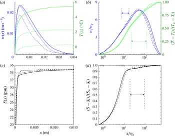
Simulations for initially uniform surroundings were run for a range of field temperatures and salinities. We consider the flow only at times when the bulk of the interior is unaffected by the outflow at the top and the bottom of the domain. Figure 1(b) shows the temporal evolution of interface temperature and dissolution velocity, at mid-depth, for far-field temperature
 $T_{w}=2.3\,^{\circ }\text{C}$
and salinity
 $S_{w}=35$
‰. The simulation begins with no flow apart from an imposed small amplitude of white noise in the velocity field decreasing exponentially with distance from the ice face over 1 mm. The interface temperature and salinity are initially set equal to far-field conditions. At early times during the formation of a boundary layer, dissolution is rapid. The dissolution velocity decreases rapidly and reaches a statistically steady value after approximately 20 s. In the steady state both interface temperature and dissolution velocity show a high-frequency variability. Interface salinity is tied to interface temperature and shows a similar temporal behaviour.
Snapshots of flow solution for the case of the far-field temperature
 $T_{w}=2.3\,^{\circ }\text{C}$
and salinity
 $S_{w}=35$
‰ at time
 $t=72~\text{s}$
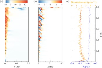
after flow field reaches quasi-steady state. Plots show the instantaneous (a)
 $w$
(
 $\text{mm}~\text{s}^{-1}$
) and (b)
 $v$
(
 $\text{mm}~\text{s}^{-1}$
) on a vertical
 $x$
–
 $z$
plane and (c) vertical profiles of
 $T_{i}$
(
 $^{\circ }\text{C}$
) and
 $|V|$
(
 ${\rm\mu}\text{m}~\text{s}^{-1}$
) at
 $y=0.025~\text{m}$
, along with the spanwise and time-averaged profile of
 $|V|$
(red dashed-dot).

Less saline water released from the interface moves upward and forms a boundary layer adjacent to the ice face (figure 2
a,b). A bidirectional flow field is set up on the lower portion of the ice face, as previously observed in laboratory experiments at similar conditions (Josberger & Martin Reference Josberger and Martin1981). Nilson (Reference Nilson1985) provided a flow-regime map in terms of the buoyancy ratio
 $R_{{\it\rho}}$
and Lewis number
 $Le={\it\kappa}_{T}/{\it\kappa}_{S}$
. By comparison to our present parameter regimes some cases with low ambient temperature would be expected to show counterflow where the inner upward flow is dominant. In this lower region there is a narrow and laminar boundary layer flow with thickness
 $O(0.1)~\text{mm}$
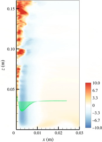
immediately adjacent to the ice face bounded on the outer side by a wider downward flow of thickness of 8–10 mm, as seen at the lower portion of the iceblock in figure 3. At the bottom boundary of the box the downward flow forms an outflow from the ice face. The outer boundary layer grows wider with decreasing
 $z$
but remains laminar. Transition from laminar to turbulent flow occurs in the inner boundary layer at a height of 60–80 mm from the bottom of the box. This inner layer becomes fully turbulent above 100 mm from the bottom boundary, generating large horizontal velocities, as shown in figure 2(b), where we defined the fully developed turbulent region above the height where spanwise fluctuations (
 $v_{rms}$
) reach 10 % or more of the average upward flow and then found the time average at that height. The critical Grashof number for this kind of buoyancy-driven flow against a vertical surface is
 $Gr_{cr}\sim 10^{9}$
(Turner Reference Turner1973), which in our problem corresponds to height
 $H_{cr}\sim 10$
–
 $30~\text{cm}$
depending on the ambient conditions, as consistent with previous experiments (Josberger & Martin Reference Josberger and Martin1981; Carey & Gebhart Reference Carey and Gebhart1982; Johnson & Mollendrof Reference Johnson and Mollendrof1984; McConnochie & Kerr Reference Mcconnochie and Kerr2016). For a given far-field salinity
 $S_{w}$
, upflow becomes turbulent at smaller
 $z$
for larger far-field temperatures
 $T_{w}$
, reflecting faster dissolution for higher
 $T_{w}$
.
Enlarged view of an instantaneous vertical velocity field (
 $\text{mm}~\text{s}^{-1}$
) of figure 2 near the bottom corner of the box, again on a vertical
 $x$
–
 $z$
plane. A profile of
 $w$
is shown at a height of
 $z=0.035~\text{m}$
.

The boundary layer structure also influences the dissolution velocity. In the laminar regime the dissolution velocity is smaller due to a thicker thermal boundary layer. In the transition region the interface temperature and dissolution velocity increase rapidly with height from the bottom of the box. For the solution in figure 2 the dissolution velocity reaches a maximum at
 $z\sim 70~\text{mm}$
. The location of most rapid dissolution is close to the upper limit of the outer downward flow and is likely to cause the formation of a notch in the ice surface, as previously reported in experiments by Josberger & Martin (Reference Josberger and Martin1981). Above this depth the dissolution velocity decreases gradually and becomes independent of height in the fully turbulent boundary layer region, where the flow is also unidirectional.
Small, high-frequency transient fluctuations in the dissolution rate are caused by turbulent motions next to the ice face. The time averaged solutions in the turbulent boundary layer region show no spanwise variation and no significant vertical variation of the dissolution rate (figure 2 c). An absence of spanwise structure on the melting ice face or spanwise variation of melt rate was also note in previous experiments (Josberger & Martin Reference Josberger and Martin1981; Carey & Gebhart Reference Carey and Gebhart1982; Kerr & McConnochie Reference Kerr and Mcconnochie2015).
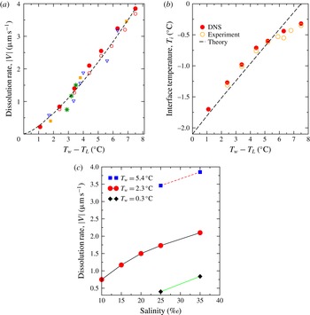
The dissolution velocities and interface temperatures depend on far-field conditions, as illustrated in figure 4 (where both quantities have been averaged over time and over the interface area in the turbulent boundary layer region
 $0.4~\text{m}\leqslant z\leqslant 0.95~\text{m}$
for the long-time statistically steady flow). Larger ambient temperature enhances the heat transfer rate and, hence, increases the dissolution velocity monotonically (figure 4
a). The interface temperature (figure 4
b) also increases with ambient temperature. At ambient temperatures below
 $0\,^{\circ }\text{C}$
dissolution occurs as a result of depression of the freezing point by diffusion of salt to the interface (Woods Reference Woods1992; Kerr & McConnochie Reference Kerr and Mcconnochie2015).
Depth- and time-averaged dissolving velocities (a) and interface temperatures (b) as a function of the temperature difference
 $T_{w}-T_{L}$
, and (c) dissolving velocities replotted as function of far-field salinity
 $S_{w}$
at fixed far-field temperatures
 $T_{w}=0.3$
, 2.3,
 $5.4\,^{\circ }\text{C}$
. In (a) and (b) symbols indicate far-field conditions: ●, DNS
 $S_{w}=35$
‰; ▪, DNS
 $S_{w}=25$
‰ (
 $T_{w}=0.3$
, 2.3,
 $5.4\,^{\circ }\text{C}$
);
 $\ast$
, DNS
 $T_{w}=2.3\,^{\circ }\text{C}$
(
 $S_{w}=10$
, 15, 25 ‰); experimental values (○, Kerr & McConnochie Reference Kerr and Mcconnochie2015; ▿, Josberger & Martin Reference Josberger and Martin1981); – –, theoretical prediction (3.1) for
 $S_{w}=35$
‰. (Experiments had a range of 29 ‰
 ${\leqslant}S_{w}\leqslant 35$
‰.)

Dissolution velocity monotonically increases with increasing ambient salinity (figure 4
c) at fixed ambient temperature. A larger ambient salinity leads to a larger diffusive salt flux inside the boundary layer and a larger salinity at the ice interface. The effect is nonlinear with
 $S_{w}$
because there is a limit to the freezing point depression. The freezing point depression increases the temperature gradient, enhances the heat transfer rate, hence increasing dissolution velocity. The result (figure 4
a) shows that the dissolution velocity is dependent predominantly on the driving difference
 $T_{w}-T_{L}$
, where
 $T_{L}$
is the freezing point temperature corresponding to the ambient salinity
 $S_{w}$
. The DNS results agree well with previous experiments (Josberger & Martin Reference Josberger and Martin1981; Kerr & McConnochie Reference Kerr and Mcconnochie2015). Applying the theory of Kerr & McConnochie (Reference Kerr and Mcconnochie2015) for NaCl solutions and neglecting heat transfer though the ice, we predict a dissolution velocity
 $$\begin{eqnarray}|V|\approx (0.250\pm 0.002)(T_{w}-T_{L})^{1.352\pm 0.004}~{\rm\mu}\text{m}~\text{s}^{-1},\end{eqnarray}$$
for
 $T_{w}\leqslant 6\,^{\circ }\text{C}$
and 30 ‰
 ${\leqslant}S_{w}\leqslant 35$
‰.
(a) Profiles of averaged vertical velocity and temperature as function of distance from the interface at mid-depth for three ambient temperatures at a fixed ambient salinity
 $S_{w}=35$
‰. Averaging is over time and spanwise direction. (b) Normalised velocity and temperature from (a) with logarithmic distance from the ice. Results are for
 $T_{w}=5.4\,^{\circ }\text{C}$
(continuous lines),
 $2.3\,^{\circ }\text{C}$
(dashed) and
 $0.3\,^{\circ }\text{C}$
(dash-dot), respectively. Arrows show logarithmic region. Similarly profiles of averaged salinity are shown in dimensional and normalised forms in (c) and (d), respectively.

Profiles of vertical velocity at mid-depth are shown in figure 5 for three ambient temperatures and the same far-field salinity. The profiles are broader and the flow is faster for higher ambient temperature. These profiles collapse approximately to a single universal profile when velocity is normalized by the buoyancy velocity scale,
 $w_{g}=[g{\it\beta}(S_{w}-S_{i}){\it\kappa}_{S}]^{1/3}$
, distance from the interface is normalised by
 ${\it\eta}_{g}=[{\it\kappa}_{S}^{2}/g{\it\beta}(S_{w}-S_{i})]^{1/3}$
. Temperature and salinity are expressed as
 $(T-T_{i})/(T_{w}-T_{i})$
and
 $(S-S_{i})/(S_{w}-S_{i})$
, respectively. This scaling is that previously found to apply to turbulent boundary layer convection on a heated vertical wall (George & Capp Reference George and Capp1979). The scaled temperature and salinity reach approximately
 $80\,\%$
and
 $95\,\%$
of its far-field values at the location of maximum vertical velocity. Both velocity and temperature show logarithmic profiles (within intervals marked in figure 5
b) in the inner boundary layer, and the logarithmic behaviour of the temperature profiles extends beyond the inner region, as observed for turbulent natural convection at a heated vertical surface (Tsuji & Nagano Reference Tsuji and Nagano1989). We have also calculated the buoyancy given by (2.5). The salinity contribution is an order of magnitude larger than that of temperature and therefore there is no significant difference between the profiles of buoyancy and salinity.
Key quantities averaged in time, spanwise and across the boundary layer width: (a) vertical velocity
 $\langle w\rangle$
(
 $\text{m}~\text{s}^{-1}$
), (b) volume flux
 $\langle Q\rangle$
(
 $\text{m}^{2}~\text{s}^{-1}$
), (c) momentum flux
 $\langle M\rangle$
(
 $\text{m}^{3}~\text{s}^{-2}$
) and (d) buoyancy
 $\langle {\it\Delta}\rangle$
(
 $\text{m}~\text{s}^{-2}$
), as functions of height for three cases with buoyancy flux per unit area
 ${\it\Phi}=1.61\times 10^{-6}~\text{m}^{2}~\text{s}^{-3}$
,
 $1.38\times 10^{-6}~\text{m}^{2}~\text{s}^{-3}$
and
 $1.89\times 10^{-7}~\text{m}^{2}~\text{s}^{-3}$
(upper to lower data sets, respectively). The
 ${\it\Phi}$
values are calculated directly from the interfacial buoyancy fluxes. Dashed lines show the predicted value of as discussed in the text.

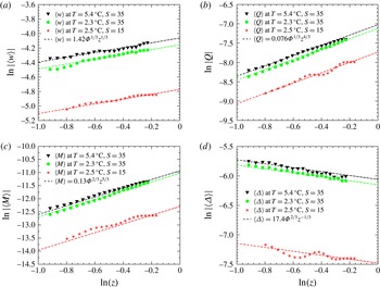
The height dependence of the flow is shown in figure 6, as represented by averaged vertical velocity
 $\langle w\rangle$
, volume flux
 $\langle Q\rangle$
, momentum flux
 $\langle M\rangle$
and averaged buoyancy,
 $\langle {\it\Delta}\rangle$
, where
 ${\it\Delta}=-g({\it\rho}_{p}-{\it\rho}_{w})/{\it\rho}_{0}$
is based on averaged plume density
 ${\it\rho}_{p}(z)$
and ambient density
 ${\it\rho}_{w}$
. These results can be compared with a theoretical model of a vertical natural convective boundary layer on a heated isothermal surface (Wells & Worster Reference Wells and Worster2008) and with a theoretical model a wall plume driven by a uniformly distributed wall buoyancy flux
 ${\it\Phi}$
giving boundary layer flux
 $F=z{\it\Phi}$
(Cooper & Hunt Reference Cooper and Hunt2010). These models assumed top-hat profiles across the plume and a uniform ambient. From Cooper & Hunt (Reference Cooper and Hunt2010) the predicted scaling is for vertical velocity
 $\langle w\rangle =c_{w}{\it\Phi}^{1/3}z^{1/3}$
, volume flux
 $\langle Q\rangle =c_{Q}{\it\Phi}^{1/3}z^{4/3}$
, momentum flux
 $\langle M\rangle =c_{M}{\it\Phi}^{2/3}z^{5/3}$
, and boundary layer buoyancy
 $\langle {\it\Delta}\rangle =c_{{\it\Delta}}{\it\Phi}^{2/3}z^{-1/3}$
. McConnochie & Kerr (Reference Mcconnochie and Kerr2016) revisited this theory in the context of their ice-dissolving experiments concluded that there is a large frictional stress, which is neglected in Cooper & Hunt (Reference Cooper and Hunt2010). The present simulations allow us to evaluate the frictional stress, which we find to be 65 % of the buoyancy force. Most of this frictional stress comes from the viscous drag at the wall (85 % of the total frictional stress), and the reminder is from the turbulent motions within the plume. Both of the frictional components follow the same scaling with height as the buoyancy force within the plume. The model of Cooper & Hunt (Reference Cooper and Hunt2010) can be modified to include friction by writing the momentum equation (from their equation (2.2)) as
 $$\begin{eqnarray}\frac{\text{d}\langle M\rangle }{\text{d}z}=\frac{\langle Q\rangle F}{\langle M\rangle }-{\it\varepsilon}_{F}.\end{eqnarray}$$
Here, the frictional stress
 ${\it\varepsilon}_{F}$
can be modelled by
 ${\it\varepsilon}_{F}=\overline{c}_{D}\langle w\rangle ^{2}$
using a mean drag coefficient
 $c_{D}$
and mean vertical velocity
 $\langle w\rangle$
. The scaling solutions for
 $\langle w\rangle$
,
 $\langle Q\rangle$
,
 $\langle M\rangle$
and
 $\langle {\it\Delta}\rangle$
are as in Cooper & Hunt (Reference Cooper and Hunt2010), (equation (2.3)), while the prefactors are modified and expressed as
 $$\begin{eqnarray}\left.\begin{array}{@{}cc@{}}c_{w}^{\ast }=c_{w}\left(1+\displaystyle \frac{4\overline{c}_{D}}{5{\it\alpha}_{e}}\right)^{-1/3}, & \quad c_{Q}^{\ast }=c_{Q}\left(1+\displaystyle \frac{4\overline{c}_{D}}{5{\it\alpha}_{e}}\right)^{-1/3},\\ c_{M}^{\ast }=c_{M}\left(1+\displaystyle \frac{4\overline{c}_{D}}{5{\it\alpha}_{e}}\right)^{-2/3}, & \quad c_{{\it\Delta}}^{\ast }=c_{{\it\Delta}}\left(1+\displaystyle \frac{4\overline{c}_{D}}{5{\it\alpha}_{e}}\right)^{1/3}.\end{array}\right\}\end{eqnarray}$$
Here,
 ${\it\alpha}_{e}$
is the entrainment coefficient. Our simulations (after integration of the profiles across the boundary layer) show the same depth-dependence and directly provide the constant prefactors
 $c_{w}^{\ast }\approx 1.42$
,
 $c_{Q}^{\ast }\approx 0.076$
,
 $c_{M}^{\ast }\approx 0.13$
and
 $c_{{\it\Delta}}^{\ast }\approx 17.4$
, which are comparable to those inferred from the experiments (McConnochie & Kerr Reference Mcconnochie and Kerr2016). We also estimate
 $\overline{c}_{D}=0.18$
for parameterisation based on averaged velocity across the boundary layer and
 $c_{D}=0.06$
based on the maximum velocity. Such a large drag coefficient is reasonable as the buoyancy induced velocity has a peak value very close to the wall. The wall friction explains the relatively small velocity and momentum flux in both the simulation and experiment compared with those given by the model of Cooper & Hunt (Reference Cooper and Hunt2010), where
 $c_{w}\sim 2.98$
and
 $c_{M}\sim 0.2$
. In some respects our present set-up is also different from the experiments of Cooper & Hunt (Reference Cooper and Hunt2010). Their experiments involve the supply of buoyant fluid though a semipermeable membrane, whereas the present case has buoyancy diffusing from the boundary and forming a distinct laminar sublayer and a different compositional gradient normal to the wall.
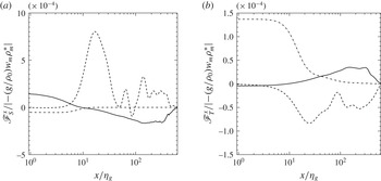
The buoyancy flux in each of the vertical and horizontal directions can be decomposed into mean advective, turbulent and molecular diffusive components. The results in the horizontal direction are shown in figure 7. Profiles of mean advective salinity buoyancy flux show interesting behaviour that is always away from the wall in the viscous sublayer (due to the ablation velocity given the reference frame being used) but becomes inward in the rest of the boundary layer. The horizontal turbulent buoyancy flux is a dominant contribution outside the viscous sublayer. Diffusive flux of salt plays a significant role in the viscous sublayer next to the ice face with a peak at the interface and decays very rapidly beyond this sublayer. We define the horizontal turbulent diffusivity for salinity
 ${\it\kappa}_{S,x}^{tur}=-\overline{u^{\prime }S^{\prime }}/(\text{d}\overline{S}/\text{d}x)$
and temperature
 ${\it\kappa}_{T,x}^{tur}=-\overline{u^{\prime }T^{\prime }}/(\text{d}\overline{T}/\text{d}x)$
based on turbulent fluxes and mean gradients in the wall-normal direction and find
 ${\it\kappa}_{T,x}^{tur}/{\it\kappa}_{T}\sim 100$
–200 and
 ${\it\kappa}_{S,x}^{tur}/{\it\kappa}_{S}\sim 150$
–250 in the turbulent boundary layer. Here the mean (overbar) and fluctuating (primed) components are evaluated in the spanwise
 $y$
direction. Mean salinity buoyancy flux (
 $-g\overline{w}{\it\beta}(\overline{S}-S_{w})$
) is the main source of buoyancy transport in the vertical direction, and is always upward throughout the boundary layer. Its peak appears slightly closer to the ice interface than does the maximum upward mean velocity (not shown here). The profile of thermal buoyancy flux is similar to the mean salinity flux but is always downward. The turbulence component of the buoyancy flux
 $-(g/{\it\rho}_{0})\overline{w^{\prime }{\it\rho}^{\prime }}$
has a negligible role in the buoyancy transport in the vertical direction.
Profiles of averaged horizontal buoyancy flux from (a) salinity and (b) temperature anomaly as functions of normalised distance from the interface at mid-depth for fixed ambient salinity
 $S_{w}=35$
‰ and temperature
 $T_{w}=5.4\,^{\circ }\text{C}$
. Averaging is over time and spanwise direction. Results are for horizontal molecular diffusive flux (dash-dot), horizontal mean advective buoyancy flux (continuous) and turbulent buoyancy flux (dashed), respectively. Results are normalised by the maximum of profile of vertical buoyancy flux.

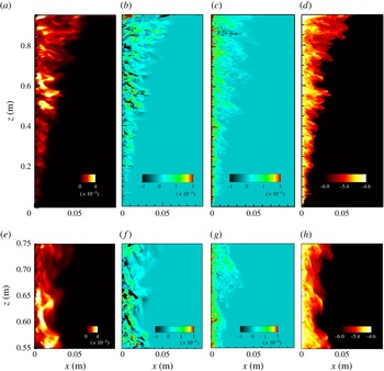
Figure 8 shows the turbulent kinetic energy field, TKE =
 $(1/2)\overline{u_{i}^{\prime }u_{i}^{\prime }}$
, buoyancy flux,
 $B=-(g/{\it\rho}_{0})\overline{{\it\rho}^{\prime }w^{\prime }}$
, turbulent production,
 $-\overline{u_{i}^{\prime }u_{j}^{\prime }}\partial \overline{u_{i}}/\partial x_{j}$
, and the turbulent dissipation,
 ${\it\varepsilon}={\it\nu}(\partial u_{i}^{\prime }/\partial x_{j})(\partial u_{i}^{\prime }/\partial x_{j})$
, where
 $u_{i}^{\prime }=u_{i}-\overline{u_{i}}$
,
 $u_{i}$
is the velocity in the
 $i$
th direction and the mean (overbar) and fluctuating (primed) velocity components are evaluated in the spanwise
 $y$
direction. The amount of TKE increases with height in the transition region and the lower portion of the turbulent boundary layer (
 $z<0.4~\text{m}$
), where the TKE is predominantly produced by the buoyancy flux. In the fully turbulent upper region TKE is supplied from both the shear production and the buoyancy flux at comparable rates, and does not continue to increase with height. Transient patches of larger TKE are observed and are maintained by shear production (which can be seen by comparing figures 8
f and 8
g). Turbulent dissipation rate is a maximum at the wall at any height, as shown in figure 8(d).
Instantaneous distribution of (a) TKE (
 $\text{m}^{2}~\text{s}^{-2}$
), (b) shear production (
 $\text{m}^{2}~\text{s}^{-3}$
), (c) turbulent buoyancy flux (
 $\text{m}^{2}~\text{s}^{-3}$
) and (d) turbulent dissipation (
 $\text{m}^{2}~\text{s}^{-3}$
expressed in log scale) in a single vertical (
 $x$
–
 $z$
) plane and a single time step for far-field temperature
 $T_{w}=2.3\,^{\circ }\text{C}$
and salinity
 $S_{w}=35$
‰. In each case the far-field value is zero. The horizontal scale is enlarged by approximately three times relative to the vertical scale in order to make the boundary layer more visible. Figures (e–h) are similar to (a–d) but focusing on the turbulent region by magnifying the vertical scale.

4 Conclusions
The first DNS of ice dissolution, allowing convection in an otherwise quiescent environment and at temperatures and salinities relevant to the polar regions, show that the diffusion of salt towards the ice–water interface depresses the freezing point and further enhances heat diffusion into the ice. Our simulations capture the complex dissolving dynamics for Grashof numbers well above the transition to fully turbulent flow inside the ascending compositional boundary layer. As previously observed in experiments, the solutions show bidirectional flow, which consists of a narrow upward flow of relatively fresh water from the ice interface and a broader downward flow of cold denser water, near the bottom of the ice face, where the flow is laminar. The flow becomes fully turbulent and unidirectional (upward) over most of the height of the box with the dissolution velocity reaching a maximum at the transition to turbulence. Over the turbulent boundary layer region dissolution velocity is nearly uniform and well predicted by theory for the dissolution of ice, which gives
 $V\sim (T_{w}-T_{L})^{4/3}$
. The computed dissolution velocities are also consistent with previous experiments with saline water. The structure of the boundary layer flow is in agreement with results for boundary layer flow on a heated vertical wall, and with the scaling for a wall plume with distributed buoyancy flux but with different scaling prefactors. The production of turbulence at the modest Grashof numbers achieved here has comparable contributions from both buoyancy and shear in the convective boundary layer. The rate of shear production is, however, expected to increase with Grashof number and future work will need to address larger scales.
In the present work our computational domain is 1 m owing to computational resources. It is also unlikely that much larger Grashof numbers will be simulated using DNS, as LES models are more suitable. Thus, the present DNS provides a valuable comparison for future modelling. Nevertheless our results show that inside the turbulent boundary layer dissolution rate is independent of the depth and magnitude of vertical velocity (figure 2 c). In recent experiments, Kerr & McConnochie (Reference Kerr and Mcconnochie2015) found a similar depth independent dissolution rate above the transition from laminar to turbulent boundary layer flow, and the results are consistent with theory for large Grashof numbers. Therefore, we expect that if the vertical scale of the ice is large enough for the flow to exceed the critical Grashof number, dissolution rate will be given by the asymptotic dynamics.
Other scaling theory (Grossmann & Lohse Reference Grossmann and Lohse2000; Wells & Worster Reference Wells and Worster2008) for both horizontal and vertical boundaries suggests the existence of a second regime of turbulent natural convection at much larger Rayleigh numbers (
 $Ra>10^{16}$
with
 $Pr=0.7$
), where small-scale turbulence and the thickness of the inner laminar subboundary layer near the wall are controlled by shear production in the convective boundary layer flow rather than by direct convective production of turbulence. In the compositional convection during ice dissolution the buoyancy if dominated by the salinity contribution and the large Schmidt number becomes the relevant parameter and the transition is predicted to occur at a salinity Rayleigh number
 $Ra\sim 10^{21}$
, which would require vertical ice heights
 $H$
of several hundreds of metres. Over such a large height other effects such as ambient stratification, the slope of the ice face and the variation of liquidus temperature with pressure will influence the dissolution rate.
Acknowledgements
Computations were carried out using the Australian National Computational Infrastructure, through the National Computational Merit Allocation Scheme supported by the Australian Government. This work was supported by Australian Research Council grants DP120102772 and DP120102744. B.G. was supported by ARC DECRA Fellowship DE140100089.