Introduction
Papers based on designed experiments appearing in agronomy and crop science journals occasionally report bivariate correlations among several traits (response variables) computed from the observed raw data. Almost invariably, these bivariate correlations are estimated and tested for significance, as Pearson's product–moment correlations, without any regard for the randomization layout or treatment structure of the experimental design. This practice is in contrast to the univariate analysis of variance (ANOVA) usually presented for the individual traits, which decomposes total variance into sources of variation due to treatments and the randomization layout. So, univariate and bivariate analyses presented in many research papers are not consistent with one another, and arguably the bivariate analyses presented violate the assumptions made in univariate ANOVA.
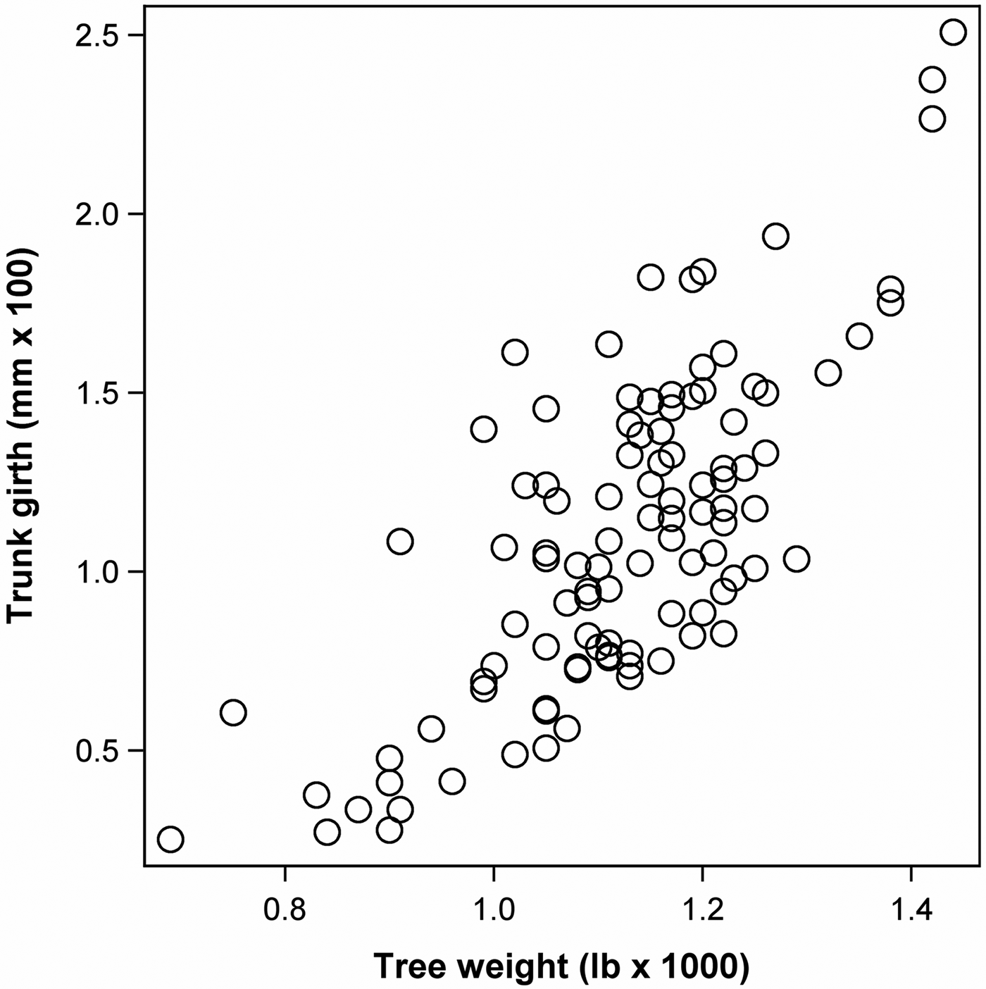
To illustrate the problem, consider data from eight apple trees for each of 13 different rootstocks (Andrews & Herzberg Reference Andrews and Herzberg1985, p. 357–360) (Example 1). Two of the traits measured were trunk girth at 4 years (mm × 100) and weight of tree above ground at 15 years (lb × 1000). The one-way ANOVA for both traits using rootstock as the treatment factor is shown in Table 1. The bivariate raw data are plotted in Fig. 1. With data from this kind of experiment, many research scientists would not hesitate to compute and test pairwise sample correlations r between traits from the observed raw data. A pairwise sample correlation (r) can be regarded as a descriptive statistic and as such is often worth reporting. Here, the sample correlation between trunk girth and tree weight is r = 0.7490 (for the benefit of readers wishing to reproduce these results using their software, results in the current tutorial paper are printed with more digits than would normally be required). When trying to interpret and further investigate this correlation, however, or testing its significance, it becomes necessary to account for the effects involved in the two traits being correlated and make meaningful distributional assumptions accounting for the presence of these effects. This all boils down to thinking carefully about a suitable bivariate model for the two traits (response variables) that are to be correlated. The usual test of significance, for example, assumes that pairs of observations on the two traits are independent, but in the case at hand pairs of data from the same rootstock are likely to be more similar than pairs from different rootstocks because they share effects of the same rootstock, thus violating the assumptions of the usual test. Note that in a univariate ANOVA, comparing the rootstocks (Table 1) requires fitting a treatment effect for rootstocks, so such an effect should also be accounted for in any bivariate analysis.
Scatter plot of trunk girth at 4 years (mm × 100) v. tree weight at 15 years (lb × 1000) for apple (Malus domestica L.) rootstock data from an experiment with 13 rootstocks (Example 1).

Univariate analyses of variance for trunk girth at 4 years (mm × 100) and tree weight at 15 years (lb × 1000) of six rootstocks of apple (Malus domestica L.) each tested on eight trees (Example 1)

In the present paper, it will be demonstrated that it is possible and useful to reconcile univariate and bivariate analyses of traits of interest and perform them in a consistent manner using mixed model procedures (Schabenberger & Pierce Reference Schabenberger and Pierce2002; Littell et al. Reference Littell, Milliken, Stroup, Wolfinger and Schabenberger2006). It will be shown how to account for treatment effects in assessing the correlation among response variables. In the next section, a bivariate model is introduced that is commensurate with the linear model used for univariate analyses (Hill & Thompson Reference Hill and Thompson1978; Singh & El-Bizri Reference Singh and El-Bizri1992; Booth et al. Reference Booth, Federer, Wells and Wolfinger2009). Based on this model, estimation of correlations and associated significance tests are described. The methods are illustrated using the rootstock example (Example 1). Three further examples serve to show a range of settings, where simple correlation might be contemplated initially, but closer investigation leads to alternative analyses, providing more insights.
Materials and methods
This section considers linear models for univariate and bivariate analysis. Several equations are given to explain how analysis of simple correlation is different from a bivariate analysis accounting for treatment and design effects and why the latter is preferable. In the development, it is assumed for simplicity that a single treatment factor has been tested according to a completely randomized design (CRD). Extension to blocked experiments is straightforward and will be illustrated using further examples.
Defining a bivariate model
The linear model underlying a univariate one-way ANOVA for an individual trait is:
 $$y_{ij} = \mu + \tau _i + e_{ij} $$
where y
ij
is the response of the jth replicate of the ith treatment, μ is a general intercept, τ
i
is the effect of the ith treatment, and e
ij
is the residual error term associated with the response y
ij
. All effects are assumed to be fixed, except the error term e
ij
, which is assumed to follow a normal distribution with zero mean and constant variance
 $\sigma _e^2 $
, i.e.
 $$e_{ij}\sim N \left( {0,\sigma _e^2 } \right)$$
where
 $N\left( {0,\sigma _e^2} \right)$
represents a normal distribution, the first argument denoting the mean (0 in this case) and the second argument denoting the variance (
 $\sigma _e^2 $
in this case). The expected value, or mean, of the response y
ij
for a given treatment i is E(y
ij
) = μ + τ
i
. Thus, the response has an assumed normal distribution with mean μ + τ
i
, comprised the fixed effects of the model, and variance
 $\sigma _e^2 $
, which in short-hand notation can be written as
 $$y_{ij}\sim N \left( {\mu + \tau _i,\sigma _e^2 } \right)$$
The natural starting point for bivariate analysis is the model used for univariate ANOVA. It seems reasonable to require that the model holding for univariate ANOVA of each individual trait is also implied by any bivariate model contemplated for the joint analysis of two traits. In other words, the bivariate model should be a natural extension of the univariate model. Thus, model (1) may be assumed to hold for both traits simultaneously. All the effects will need to be trait-specific, of course, so all effects are indexed by traits. For two traits 1 and 2, the two univariate models then are written as:
 $$y_{ij1} = \mu _1 + \tau _{i1} + e_{ij1} $$
and
 $$y_{ij2} = \mu _2 + \tau _{i2} + e_{ij2} $$
The errors are assumed to have zero mean and trait-specific variances:
 $${\mathop{\rm var}} (e_{ij1} ) = \sigma _{e(1)}^2 $$
and
 $${\mathop{\rm var}} (e_{ij2} ) = \sigma _{e(2)}^2 $$
In addition, now that a bivariate analysis is considered, the correlation among traits also needs to be accounted for. Errors for observations on the two traits made on the same plot can be assumed to be correlated with covariance:
 $${\mathop{\rm cov}} (e_{ij1}, e_{ij2} ) = \sigma _{e(1,2)} $$
The correlation is defined as:
 $${\rm corr}(e_{ij1}, e_{ij2} ) = \rho _{e(1,2)} = \displaystyle{{\sigma _{e(1,2)}} \over {\sigma _{e(1)} \sigma _{e(2)}}} $$
For bivariate analysis it is convenient to collect effects of the same type into vectors of length two, allowing Eqns (4) and (5) to be written more compactly as
 $$\left( {\matrix{ {y_{ij1}} \cr {y_{ij2}} \cr}} \right) = \left( {\matrix{ {\mu _1} \cr {\mu _2} \cr}} \right) + \left( {\matrix{ {\tau _{i1}} \cr {\tau _{i2}} \cr}} \right) + \left( {\matrix{ {e_{ij1}} \cr {e_{ij2}} \cr}} \right)$$
A short-hand notation for the distributional assumption for the errors then is
 $$\left( {\matrix{ {e_{ij1}} \cr {e_{ij2}} \cr } } \right)\sim BVN \left[ {\varphi = \left( {\matrix{ 0 \cr 0 \cr } } \right),\Sigma = \left( {\matrix{ {\sigma _{e(1)}^2 } & {\sigma _{e(1,2)}} \cr {\sigma _{e(1,2)}} & {\sigma _{e(2)}^2 } \cr } } \right)} \right]$$
where BVN(φ, Σ) represents a bivariate normal distribution, with the first argument (φ) denoting the mean vector (here, means for both e
ij1 and e
ij2 are zero) and the second (Σ) the variance-covariance matrix with the two variances
 $\sigma _{e(1)}^2 $
and
 $\sigma _{e(2)}^2 $
on the diagonal and the covariance σ
e(1,2) on the off-diagonal. With this assumption, the distributional model for the observed data can be stated as:
 $$\left( {\matrix{ {y_{ij1}} \cr {y_{ij2}} \cr } } \right)\sim BVN \left[ {\left( {\matrix{ {\mu _1 + \tau _{i1}} \cr {\mu _2 + \tau _{i2}} \cr } } \right),\left( {\matrix{ {\sigma _{e(1)}^2 } & {\sigma _{e(1,2)}} \cr {\sigma _{e(1,2)}} & {\sigma _{e(2)}^2 } \cr } } \right)} \right]$$
It is important to note that the bivariate distributional model (12) is consistent with the assumption that the univariate distributional model (3) holds for each of the two traits because both comprise the same set of parameters (effects and variances).
It may now be asked: what is the implicit assumption for the distribution of the bivariate observations (y ij1, y ij2), if simple sample correlations r are computed from the observed data and subjected to a significance test? The answer is that we are effectively assuming that the paired observations are a simple random sample from the same (!) population, implying this bivariate model:
 $$\left( {\matrix{ {y_{ij1}} \cr {y_{ij2}} \cr } } \right)\sim BVN \left[ {\left( {\matrix{ {\mu _1} \cr {\mu _2} \cr } } \right),\left( {\matrix{ {\sigma _{e(1)}^2 } & {\sigma _{e(1,2)}} \cr {\sigma _{e(1,2)}} & {\sigma _{e(2)}^2 } \cr } } \right)} \right]$$
In particular, this is the assumption needed for the classical t-test of the null hypothesis that the two traits are uncorrelated, based on the test statistic
 $t = r\sqrt {n - 2} /\sqrt {1 - r^2} $
where n is the sample size, or the equivalent F-statistic F = t
2 (Mead et al.
Reference Mead, Curnow and Hasted1993). So, when simple correlations are computed and tested, the treatment effects implicitly drop out of the model! From the development of the bivariate model (12) as a natural extension of the univariate model (1), however, it is clear that the simple model (13) violates the distributional assumption made about each individual trait in a univariate ANOVA. Specifically, under model (12), each observation vector (y
ij1, y
ij2) has its own expected value (μ
1 + τ
i1, μ
2 + τ
i2), as opposed to (13), where all observation vectors have the same expectation (μ
1, μ
2). For this reason, model (13) is not tenable for data from a designed experiment, yet many researchers readily assume that model, presumably often without realizing, when computing pairwise correlations from plot data and performing significance tests on them. Subsequently, a method to estimate bivariate correlations will be outlined that takes treatment effects into account. Before doing so, the related problem of assessing the importance of the variability of treatment effects for single traits will be considered. This is done to motivate the approach proposed for bivariate analysis.
Defining and estimating variance and covariance for treatment effects
When computing a marginal correlation for the bivariate observation vector (y ij1, y ij2) in a designed experiment, the effects of the model must be taken into account. Rather than thinking directly in terms of a correlation of the observed data, one may consider correlations at the level of each of the effects in the model. Here is where the bivariate formulation is given in Eqn (10) comes in handy. For a CRD, there are two bivariate vectors of effects that vary across the data, i.e. treatment effects (τ i1, τ i2) and residual errors (e ij1, e ij2). The important point here is that a bivariate correlation for each of these bivariate effects should be expected.
As a prelude to defining a general procedure for estimating bivariate correlations in designed experiments, taking all effects into account, this section considers the problem of estimating a variance of treatment effects for a single trait and the related problem of estimating a covariance of treatment effects for two traits. It will be argued that it is both reasonable and convenient for this particular purpose to consider treatment effects as random and estimate variances and covariances using residual maximum likelihood (REML) (Patterson & Thompson Reference Patterson and Thompson1971; Searle et al. Reference Searle, Casella and McCulloch1992), even in situations where the treatment effect would normally be regarded as fixed. To justify the approach, a variance estimator for a balanced one-way layout as in Example 1 will first be introduced under the assumption of fixed treatment effect. Next, it will be stressed that this estimator coincides with that obtained under a random-effects model. Subsequently, the equivalence of estimators under the fixed and random assumptions will also be demonstrated for the covariance.
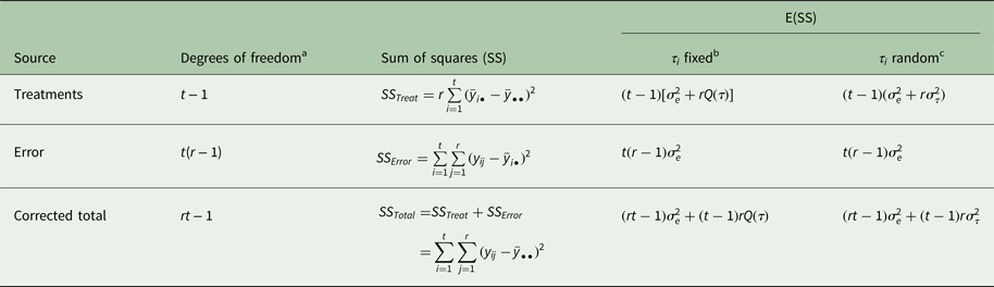
The one-way ANOVA has two sources of variation, corresponding to the two effects in the model, i.e. treatments τ i and error e ij . Table 2 shows the sums of squares of a one-way ANOVA with t treatments and r replications per treatment. It may be of interest to quantify the importance of treatment effects in relation to the total variation. A possible measure is the ‘sample variance’, or finite-population variance, of the fixed treatment effects, given by:
 $$Q(\tau ) = \displaystyle{{\sum\nolimits_{i = 1}^t {(\tau _i - \bar \tau _ \bullet )^2}} \over {t - 1}}$$
where
 $\bar {\hskip-2pt\tau} _ \bullet $
denotes the arithmetic mean of the treatment effects τ
i
.
Variance parameter estimates for the apple (Malus domestica L.) rootstock data in Table 1 (Example 1) under the hypotheses H A : ρ y(1,2) ≠ 0
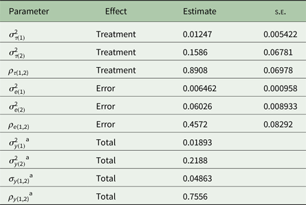
Trait 1 = trunk girth at 4 years (mm × 100), trait 2 = tree weight at 15 years (lb × 1000).
a These values were read off the output of the statistical package and are slightly different from the values one would obtain by plugging the estimates of variances and covariances for the effects shown in this table, which are rounded to the forth decimal place, into Eqns (26)–(28) for the marginal variances, covariance and correlation.
This is a natural measure to quantify the variability of the fixed treatment effects (Winer et al. Reference Winer, Brown and Michels1991; Gelman Reference Gelman2005). Q(τ) can be estimated from the two ANOVA mean squares as
 $$\hat {\hskip-1ptQ} (\tau ) = \displaystyle{{MS_{treat} - MS_{error}} \over r}$$
where MS
treat
= SS
treat
/(t − 1), MS
error
= SS
error
/[t(r − 1)], with treatment and error sums-of-squares a given in Table 3. The error variance is estimated by
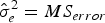 $\hat \sigma _e^2 = MS_{error} $
.
One-way ANOVA table with expected sums of squares (E(SS)) and mean squares for models with fixed and random treatment effects
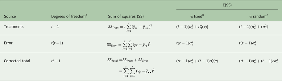
a t = number of treatments; r = number of replications per treatment.
b
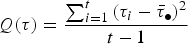 $Q(\tau ) = \displaystyle{{\sum\nolimits_{i = 1}^t {(\tau _i - \bar \tau _ \bullet )^2}} \over {t - 1}}$
; see, e.g. Winer et al. (Reference Winer, Brown and Michels1991, p. 85).
c See, e.g., Winer et al. (1991, p. 92) or Searle et al. (Reference Searle, Casella and McCulloch1992, p. 60).
So far, the treatment effect has been regarded as fixed. Since the interest here is in quantifying variability, one may alternatively consider the treatment effect as random and define a variance of treatment effects,
 $\sigma _\tau ^2 = {\mathop{\rm var}} (\tau _i )$
. Using the expected sums of squares in Table 2, the treatment variance
 $\sigma _\tau ^2 $
can be estimated from the two ANOVA mean squares as:
 $$\hat \sigma _\tau ^2 = \displaystyle{{MS_{treat} - MS_{error}} \over r}$$
This is the ANOVA or methods-of-moments estimator of the treatment variance
 $\sigma _\tau ^2 $
(Winer et al.
Reference Winer, Brown and Michels1991, p. 92; Searle et al.
Reference Searle, Casella and McCulloch1992, p. 59). Assuming normality of the treatment effects and non-negativity of the variance estimator, (16) also coincides with the REML estimator of
 $\sigma _\tau ^2 $
(Searle et al.
Reference Searle, Casella and McCulloch1992, p. 92). The important point to make here is that the estimator of Q(τ) in (15), assuming fixed treatment effects, is identical to the estimator of
 $\sigma _\tau ^2 $
in (16), assuming random effects, i.e.
 $\hat {\hskip-1pt Q}(\tau ) = \hat \sigma _\tau ^2 $
.
The same idea can be applied to define and estimate a covariance between treatment effects. Just as one can define a ‘sample variance’ Q(τ) of fixed treatment effects for a single trait, one can also define a ‘sample covariance’ of fixed treatment effects for two traits as
 $$Q(\tau _1, \tau _2 ) = \displaystyle{{\sum\nolimits_{i = 1}^t {(\tau _{i1} - \bar {\hskip-2pt\tau} _{ \bullet 1} )(\tau _{i2} - \bar {\hskip-2pt\tau} _{ \bullet 2} )}} \over {t - 1}}$$
This covariance can be estimated by the method of moments using two sums of cross-products:
 $$SP_{treat} = r\sum\limits_{i = 1}^t {(\bar y_{i \bullet 1} - \bar y_{ \bullet \bullet 1} )(\bar y_{i \bullet 2} - \bar y_{ \bullet \bullet 2} )} $$
and
 $$SP_{error} = \sum\limits_{i = 1}^t {\sum\limits_{\,j = 1}^r {(y_{ij1} - \bar y_{i \bullet 1} )(y_{ij2} - \bar y_{i \bullet 2} )}} $$
The method-of-moments estimator for (17) and the covariance of errors, σ e(1,2), are:
 $$\hat Q(\tau _1, \tau _2 ) = \displaystyle{{MP_{treat} - MP_{error}} \over r}$$
and
 $$\hat \sigma _{e(1,2)} = MP_{error} $$
where MP
treat
= SP
treat
/(t − 1) and MP
error
= SP
error
/[t(r − 1)]. When treatments are taken as random and there is a covariance between random treatment effects,
 $\sigma _{\tau (1,2)} = {\mathop{\rm cov}} (\tau _{i1}, \tau _{i2} )$
, the same estimators are obtained, i.e.
 $\hat \sigma _{\tau (1,2)} = \hat Q(\hat \tau _1, \hat \tau _2 )$
and
 $\hat \sigma _{e(1,2)} = MP_{error} $
, and these estimators coincide with the REML estimators based on a model with random treatment effects (see the following subsection), provided the variance estimates obtained from (15) are non-negative (Searle et al.
Reference Searle, Casella and McCulloch1992; Thimm Reference Thimm2002, p. 378). It is noted that sums of cross-products can be obtained conveniently from ANOVA means squares for the two traits and their sum or difference (Searle et al.
Reference Searle, Casella and McCulloch1992; Piepho et al.
Reference Piepho, Müller and Jansen2014). For example,
 $$SP_{error} = \displaystyle{{[SS_{error} (y_1 + y_2 ) - SS_{error} (y_1 ) - SS_{error} (y_2 )]} \over 2}$$
where SS error (y 1), SS error (y 2) and SS error (y 1 + y 2) denote the error sum-of-squares for the two traits and their sum, respectively.
The practical upshot of all this is that the same estimator of the variance is obtained as well as the covariance of treatment effects, no matter whether treatment effects are modelled as fixed or random. This suggests that for the purpose of estimating covariance and correlation for treatment effects, treatment effects can be taken as random and fit a bivariate model even in situations where the treatment effect would normally be taken as fixed.
The development here is for the balanced case. Residual maximum likelihood is generally applicable also to unbalanced data, and one of its advantages over an ANOVA approach is the uniqueness of the estimators (Searle et al. Reference Searle, Casella and McCulloch1992). Hence, it is desirable to generally use REML to implement the proposed procedures, which involves the explicit assumption of random effects, which will be examined below.
Decomposing the correlation using random effects
In the statement of model (1), the treatment effects were taken as fixed, and there are usually good reasons for this assumption. For example, the treatments are not usually randomly sampled from a larger population of treatments (Searle et al. Reference Searle, Casella and McCulloch1992; Gelman Reference Gelman2005). The same can often be said about the blocks, for example in a field experiment where blocks are placed adjacent to each other and their position is generally purposely selected (Dixon Reference Dixon2016). Nevertheless, based on the reasoning in the previous section, it is proposed here to take effects as random in such settings for the purpose of defining and estimating covariances and correlations among effects.
There are two possible reactions for the reader at this juncture: (1) one insists on the fixed-effects assumption and concludes that correlations can only be defined by the residual errors (e ij1, e ij2). In this case, a study of marginal correlations at the level of the observed data (y ij1, y ij2), or at the level of treatment effects (τ i1, τ i2) becomes basically meaningless, or (2) one regards the random assumption mainly as a convenient device allowing for estimates of correlation to be obtained and tested for all effects and a marginal correlation to be defined at the level of the observed data. The following considerations are based on this pragmatic view. Before proceeding, however, it should be mentioned that an alternative route to analysis observing all effects but allowing some of them to be fixed is to consider a regression analysis that uses one variate as the response and the other as a regressor variable. This option will be touched upon in Examples 3 and 4, but the focus will remain on correlation.
Assuming that all effects are random corresponds to the assumption of bivariate normality for the vectors of error and treatment effects in model (10). For the errors (e ij1, e ij2), this assumption has been specified in Eqn (11). For treatments the assumption can be stated as:
 $$\left( {\matrix{ {\tau _{i1}} \cr {\tau _{i2}} \cr } } \right)\sim BVN \left[ {\left( {\matrix{ 0 \cr 0 \cr } } \right),\left( {\matrix{ {\sigma _{\tau (1)}^2 } & {\sigma _{\tau (1,2)}} \cr {\sigma _{\tau (1,2)}} & {\sigma _{\tau (2)}^2 } \cr } } \right)} \right]$$
where
 $\sigma _{\tau (1,2)} = {\mathop{\rm cov}} (\tau _{i1}, \tau _{i2} ),\sigma _{\tau (1)}^2 = {\mathop{\rm var}} (\tau _{i1} )$
, and
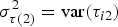 $\sigma _{\tau (2)}^2 = {\mathop{\rm var}} (\tau _{i2} )$
. With this assumption, correlations may be defined for the treatment effects as:
 $$corr(\tau _{i1}, \tau _{i2} ) = \rho _{\tau (1,2)} = \displaystyle{{\sigma _{\tau (1,2)}} \over {\sigma _{\tau (1)} \sigma _{\tau (2)}}} $$
Moreover, the marginal (total) correlation for the observed data (y ij1, y ij2) may be defined as:
 $${\rm corr}(y_{ij1}, y_{ij2} ) = \rho _{y(1,2)} = \displaystyle{{\sigma _{y(1,2)}} \over {\sigma _{y(1)} \sigma _{y(2)}}} $$
where the marginal (total) variances and the covariance of the response variables are defined as the sums of variances and covariances of the corresponding effects:
 $$\sigma _{y(1)}^2 = {\mathop{\rm var}} (y_{ij1} ) = \sigma _{\tau (1)}^2 + \sigma _{e(1)}^2 $$
 $$\sigma _{y(2)}^2 = {\mathop{\rm var}} (y_{ij2} ) = \sigma _{\tau (2)}^2 + \sigma _{e(2)}^2 $$
and
 $$\sigma _{y(1,2)} = {\mathop{\rm cov}} (y_{ij1}, y_{ij2} ) = \sigma _{\tau (1,2)} + \sigma _{e(1,2)} $$
The bivariate mixed model just described may be estimated by REML using a suitable mixed model package. Here, the GLIMMIX procedure of SAS is used. If the assumption of random effects is tenable, correlations may be tested for significance using likelihood-ratio tests (LRT). The random assumption will always be tenable for the error effects, but not necessarily for the other effects in the model. For this reason, the focus here is on the error effects and treatment effects taken as fixed, keeping them in the model throughout. Generally, the test statistic T is computed as the difference in −2 log L R between the reduced model under the null hypothesis (H 0) and the full model under the alternative (H A ), where L R is the maximized residual likelihood. Here, the H 0 is that the errors (e ij1, e ij2) are uncorrelated. In order to obtain the likelihood under H 0, the model under H 0 needs to be fitted to both traits simultaneously, constraining the covariance (or correlation) to be zero. Under the alternative H A , the covariance is allowed to differ from zero. Under the null hypothesis H 0, the test statistic has an approximate chi-squared (χ 2) distribution with degrees of freedom (d.f.) equal to the number of parameters equated to zero under H 0 (Schabenberger & Pierce Reference Schabenberger and Pierce2002). Thus, under the null hypothesis H 0 : ρ e(1,2) = 0, we set σ e(1,2) = 0, so the test statistic T has 1 d.f. One can also test the correlations of other effects by an LRT in the same way, provided the random assumption is tenable. Using the same general approach, one may also perform an LRT of the null hypothesis that error and treatment effects are equally correlated. If this null hypothesis is rejected, interpretation should focus on the correlations for effects. Otherwise, the marginal correlation provides a meaningful measure of association.
An attractive feature of the sample correlation coefficient r is that there is a simple link to the scatterplot of the data. When a bivariate mixed model is fitted, such plots can also be generated for each of the effects using their best linear unbiased predictors (BLUP). In case of the error effects, their estimators correspond to the residuals. The bivariate scatter plots for the effects can further be used to check that the association is approximately linear, which is a prerequisite for the bivariate model to be appropriate, and to inspect the degree of heterogeneity between effects in their bivariate correlations.
Extensions of the bivariate model
In the development of the bivariate mixed model, a CRD has been assumed so the model only had a treatment effect and a residual error. It is straightforward to extend the model to allow for more complex designs and covariance structures. For example, for blocked designs, the model is augmented by adding a block effect for each trait, which has a trait-specific variance and a bivariate correlation (Booth et al. Reference Booth, Federer, Wells and Wolfinger2009). It is also possible to allow for heterogeneity between treatments in the variance of error effects. Both of these extensions will be illustrated with examples.
Application to four examples
This section will look at four examples. Example 1 serves to demonstrate that treatment and error effects can have rather different correlations, in which case it is essential to inspect correlations for each type of effect. Example 2 is used to demonstrate how block effects can be incorporated into the model and that block effects can have a correlation that is rather different from that of treatment effects. Example 3 shows that there may be heterogeneity between treatments in the correlation as well as the variance of residual errors and that a regression analysis may be more informative than a simple correlation analysis. In Example 4, an experiment with subsampling on the plots is considered to demonstrate that the general approach also works with more complex mixed models and that the marginal correlation can provide a meaningful summary of the data when the residual variances are large in comparison with the variances of other effects.
Example 1 (continued)
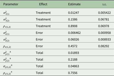
Parameter estimates for the bivariate model for the rootstock data are shown in Table 3. The marginal correlation between trunk girth at 4 years and tree weight at 15 years is estimated as
 $\hat \rho _{y(1,2)} = 0.7556$
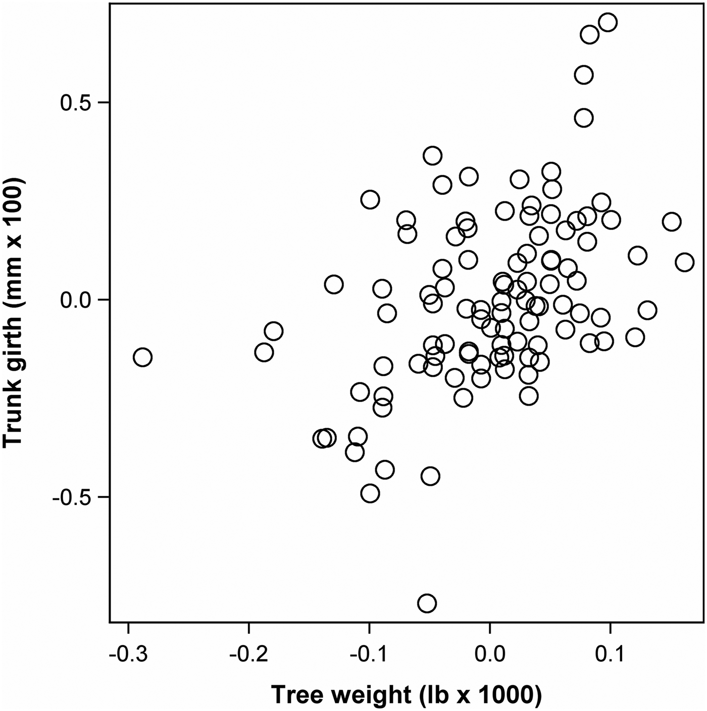
, which is rather similar, but not identical to, the sample correlation of r = 0.7490. These correlations agree with the visual impression from the scatter plot of tree weight against trunk girth in Fig. 1. By contrast, the correlation estimates for the treatment and error effects are
 $\hat \rho _{\tau (1,2)} = 0.8908$
and
 $\hat \rho _{e(1,2)} = 0.4572$
, respectively, which are rather different in value from each other and from the marginal correlation. Notably, there is a relatively high correlation between treatments, but a low correlation for errors within treatments. Taking treatment effects as fixed, the LRT of H
0 : ρ
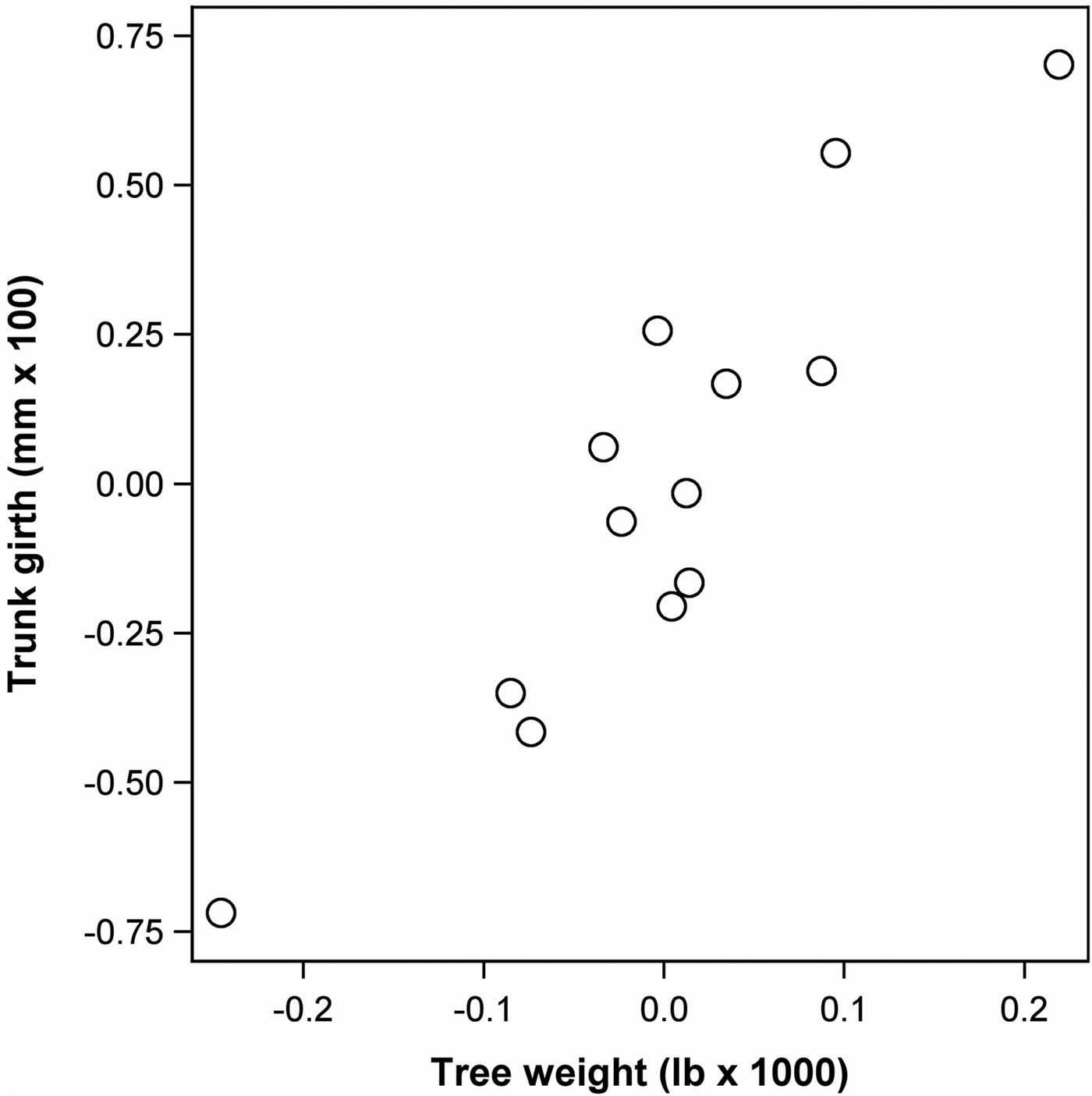
e(1,2) = 0 for residual errors is significant at the 5% level (T = 21.34, d.f. = 1, P < 0.001). The difference in correlations is also apparent from a bivariate plot of BLUPs of random treatment effects (Fig. 2) and of residuals (Fig. 3). These scatter plots show no indication of departure from linearity. A further LRT shows that treatment and error correlations are significantly different (T = 7.16, d.f. = 1, P = 0.0074). The fact that correlations are rather different for error and treatment effects underscores the importance of accounting for treatment effects when estimating correlations and suggests that the marginal correlation ρ
y(1,2) is not a very meaningful summary of the data for this example. It is more informative to focus interpretation on the treatment and error effects.
Scatter plot of BLUPs of treatment effects trunk girth at 4 years (mm × 100) v. tree weight at 15 years (lb × 1000) for apple (Malus domestica L.) rootstock data from an experiment with 13 rootstocks (Example 1).

Scatter plot of residuals for trunk girth at 4 years (mm × 100) v. tree weight at 15 years (lb × 1000) for apple (Malus domestica L.) rootstock data from an experiment with 13 rootstocks (Example 1).

The observant reader may be given to wonder why r and
 $\hat \rho _{y(1,2)} $
are different, for they seem to be estimating the same thing. The answer is that they are clearly different estimators, even if one assumes that they are estimating the same population correlation. The usual estimator r falsely assumes independence of the bivariate observations, while
 $\hat \rho _{y(1,2)} $
accounts for the correlation among bivariate observations induced by the presence of block and treatment effects. The usual estimator r is biased on account of these correlations between bivariate observations. This problem is reminiscent of, for example, the bias in the sample variance estimator in the presence of serial correlation among univariate observations (Anderson Reference Anderson1971, p. 448).
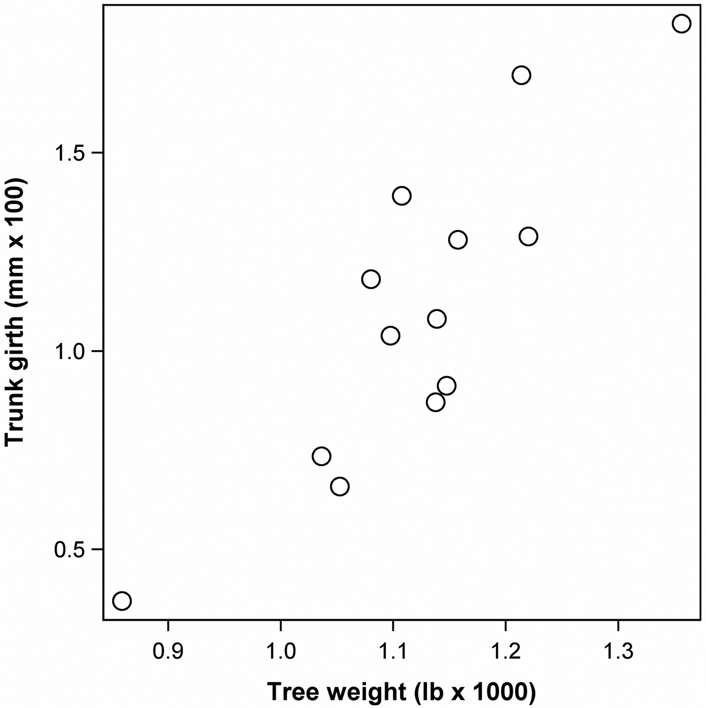
One might consider correlating observed treatment means rather than fitting a bivariate mixed model with correlated treatment effects (Fig. 4). The sample correlation of treatment means is r = 0.8675 (P < 0.001), which is lower than the estimated correlation of random treatment effects under the bivariate mixed model
 $(\hat \rho _{\tau (1,2)} = 0.8908)$
. The reason for this dilution is that sample means (i.e.
 $\bar y_{i \bullet} = \mu + \tau _i + \bar e_{i \bullet} $
) are functions not only of the treatment effects but also of the treatment averages of the residual errors, which have a considerably lower correlation
 $(\hat \rho _{e(1,2)} = 0.4572)$
than the treatment effects. This suggests that it is preferable to fit a bivariate mixed model and inspect the bivariate scatter plot of the BLUPs of treatment effects.
Scatter plot rootstock means for trunk girth at 4 years (mm × 100) v. tree weight at 15 years (lb × 1000) for apple rootstock data from an experiment with 13 apple (Malus domestica L.) rootstocks (Example 1).

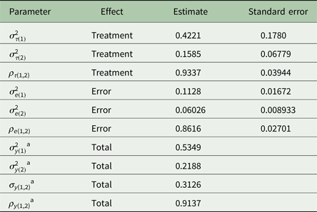
For comparison, tree weight at 15 years was jointly analysed with trunk girth at 15 (not 4!) years (Table 4). The correlations for both treatment and error effects are now rather high and also quite similar
 $(\hat \rho _{\tau (1,2)} = 0.9337\;{\rm and}\;\hat \rho _{e(1,2)} = 0.8616)$
. An LRT reveals no significant difference between the two correlations (T = 2.885, d.f. = 1, P = 0.0894), so the marginal correlation
 $(\hat \rho _{y(1,2)} = 0.9137)$
is a meaningful measure of association that is also close to the sample correlation (r = 0.9127).
Variance parameter estimates for the apple (Malus domestica L.) rootstock data in Table 1 (Example 1) under the hypotheses H A : ρ y(1,2) ≠ 0
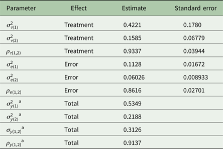
Trait 1 = trunk girth at 15 years (mm × 100), trait 2 = tree weight at 15 years (lb × 1000).
a These values were read off the output of the statistical package and are slightly different from the values one would obtain by plugging the estimates of variances and covariances for the effects shown in this table, which are rounded to the forth decimal place, into Eqns (26)–(28) for the marginal variances, covariance and correlation.
Example 2
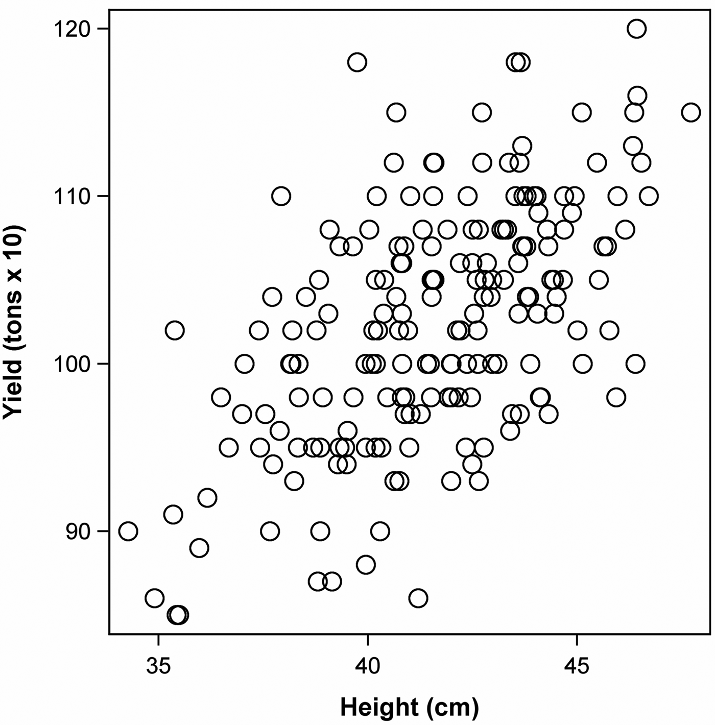
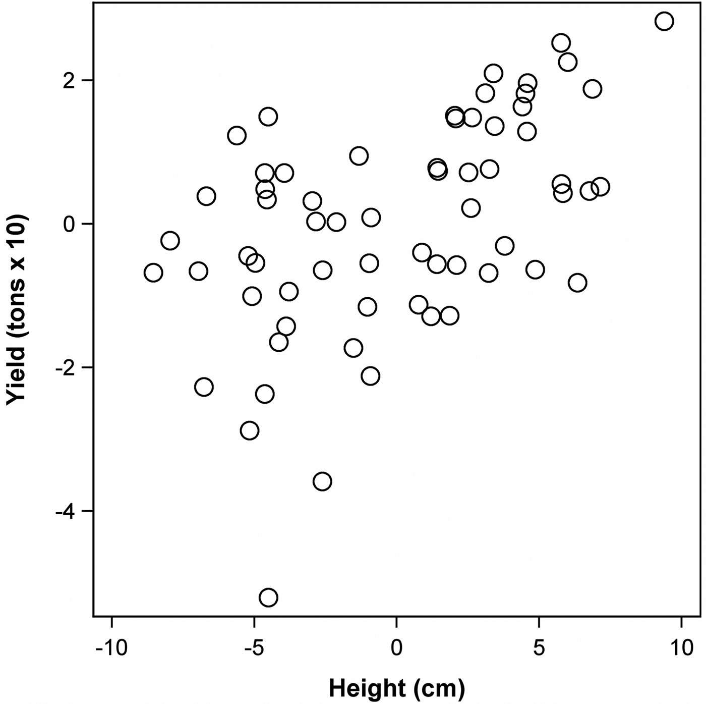
A field experiment with 64 breeding lines of oats (Avena sativa L.) was laid out as a square lattice with three replicates (Friedrich Utz, personal communication). Two of the traits assessed were yield (tonnes/ha × 10) and plant height (cm) (Fig. 5). Three outlying observations for yield were set to missing after careful inspection of residuals (it should be stressed here that outlier removal requires great care and observations should be dropped only with good justification). The sample correlation between the two traits is r = 0.5750 based on n = 189 plots with data on both traits. The following mixed model was fitted:
 $$y_{ijk} = \mu + \tau _i + r_k + b_{\,jk} + e_{ijk} $$
where y ijk is the response of the ith genotype in the jth incomplete block nested within the kth replicate. In addition to the treatment and error effects also present in (1), model (29) has an effect for the kth replicate (r k ) and for the jth incomplete block nested within the kth replicate (b jk ). The bivariate model then involves correlations not only among the treatment and error effects for both traits, but also among the replicate and incomplete block effects.
Scatter plot of yield (kg/ha) v. height (cm) for oat (Avena sativa L.) data (Example 2).

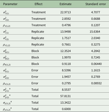
The fitted variance parameters are shown in Table 5. The estimated marginal correlation of
 $\hat \rho _{y(1,2)} = 0.6000$
is slightly larger than the sample correlation. The correlation of treatment effects is rather smaller
 $(\hat \rho _{\tau (1,2)} = 0.4796)$
, as is the correlation of error effects
 $(\hat \rho _{e(1,2)} = 0.2795)$
, whereas the correlation of block effects
 $(\hat \rho _{b(1,2)} = 0.9118)$
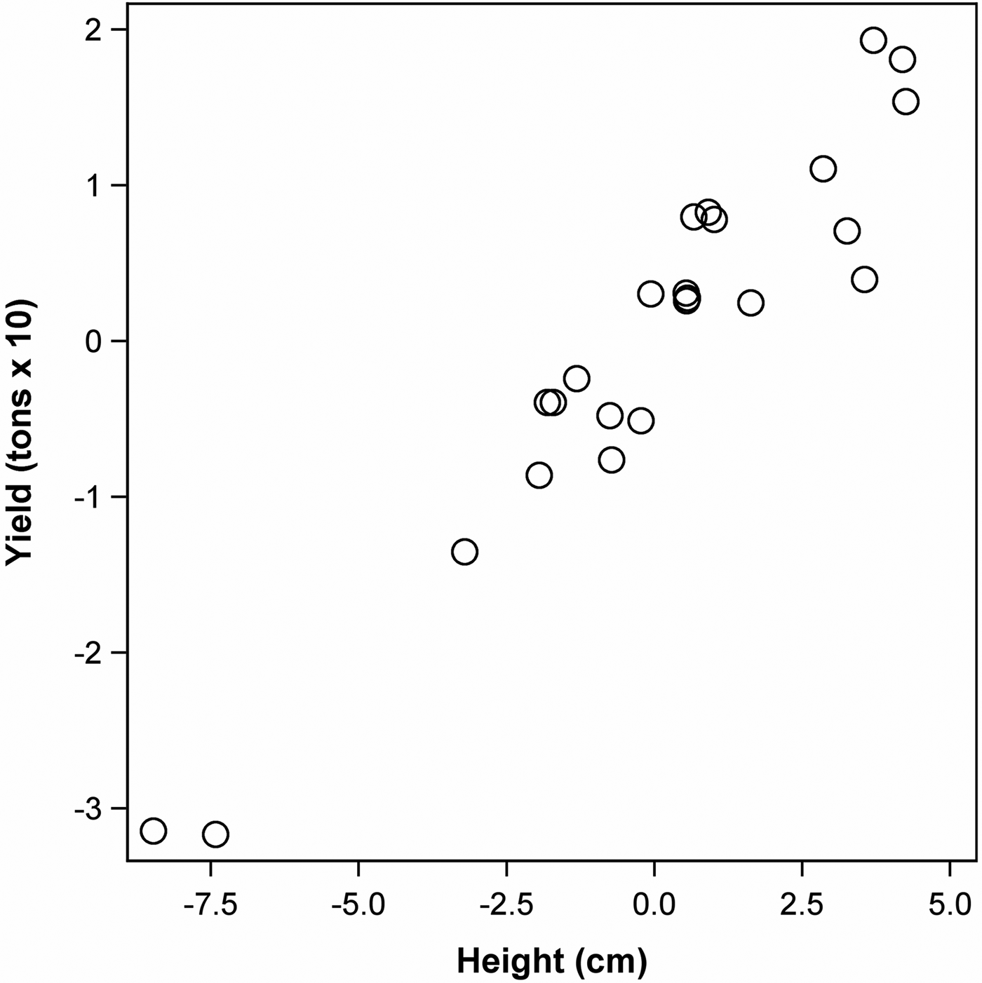
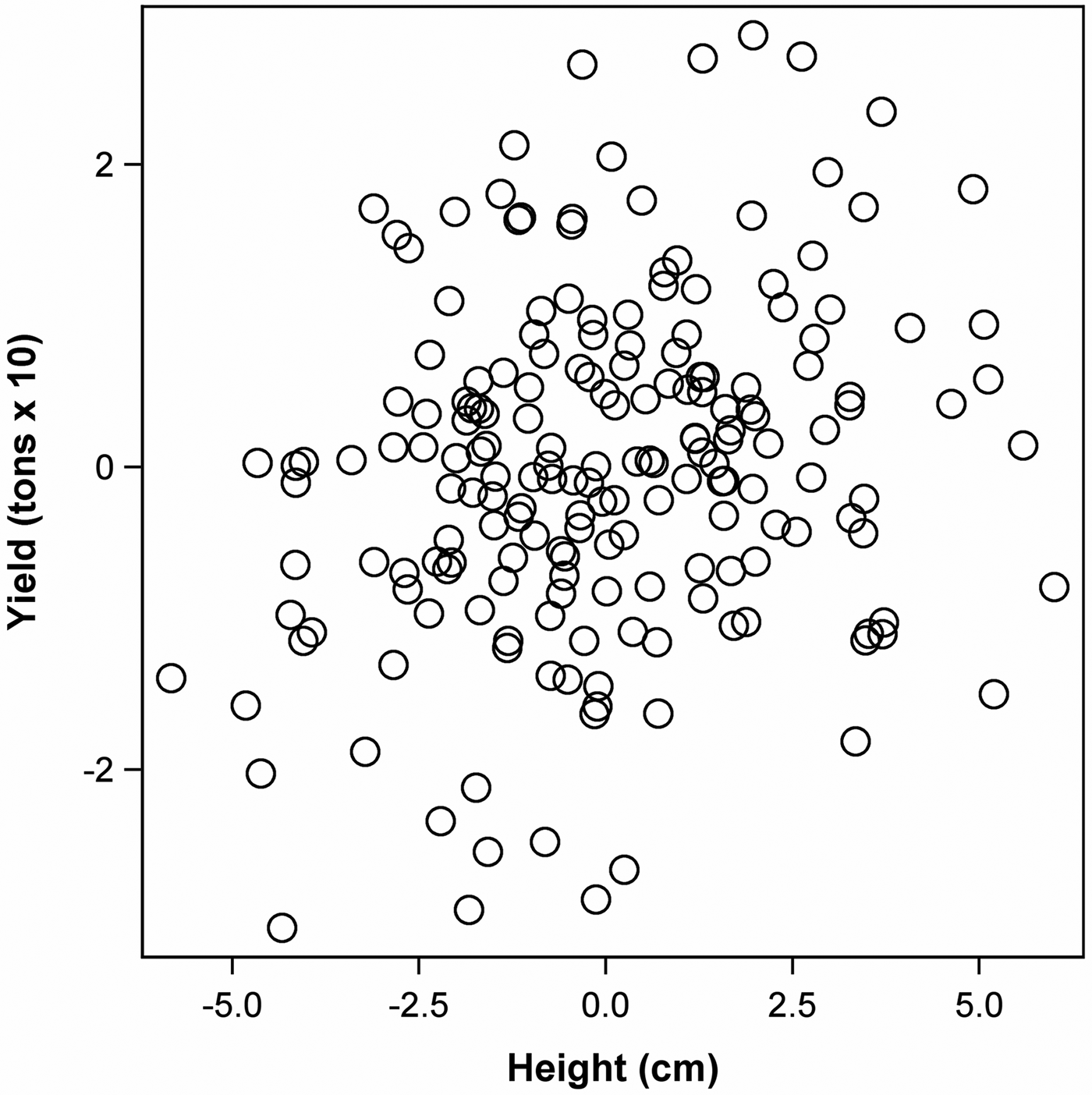
is considerably larger than both the model-based marginal correlation and the sample correlation. The bivariate scatter plots of BLUPs for effects of treatment (Fig. 6) and blocks (Fig. 7) as well as the residual plot (Fig. 8), confirm these divergent correlations. The example reinforces the observation that correlations can be quite different for different effects and it is therefore important to study correlations at the level of effects. In this application, the main interest will be in the correlation among the treatment effects because these can be used to infer if indirect selection for yield via plant height would be a more promising approach than direct selection (Falconer & Mackay Reference Falconer and Mackay1996). The relatively weak correlation for treatment effects suggests that indirect selection is not worthwhile in the case at hand.
Scatter plot of BLUPs of treatment effects for yield (kg/ha) v. height (cm) for oat (Avena sativa L.) data (Example 2).

Scatter plot of BLUPs of block effects for yield (kg/ha) v. height (cm) for oat (Avena sativa L.) data (Example 2).

Scatter plot of residuals for yield (kg/ha) v. height (cm) for oat (Avena sativa) data (Example 2).

Variance parameter estimates for oats (Avena sativa L.) data (Example 2) under the hypotheses H A : ρ y(1,2) ≠ 0
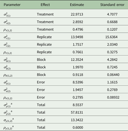
Trait 1 = yield (tonnes × 10), trait 2 = height (cm).
a These values were read off the output of the statistical package and are slightly different from the values one would obtain by plugging the estimates of variances and covariances for the effects shown in this table, which are rounded to the forth decimal place, into Eqns (26)–(28) for the marginal variances, covariance and correlation.
Example 3
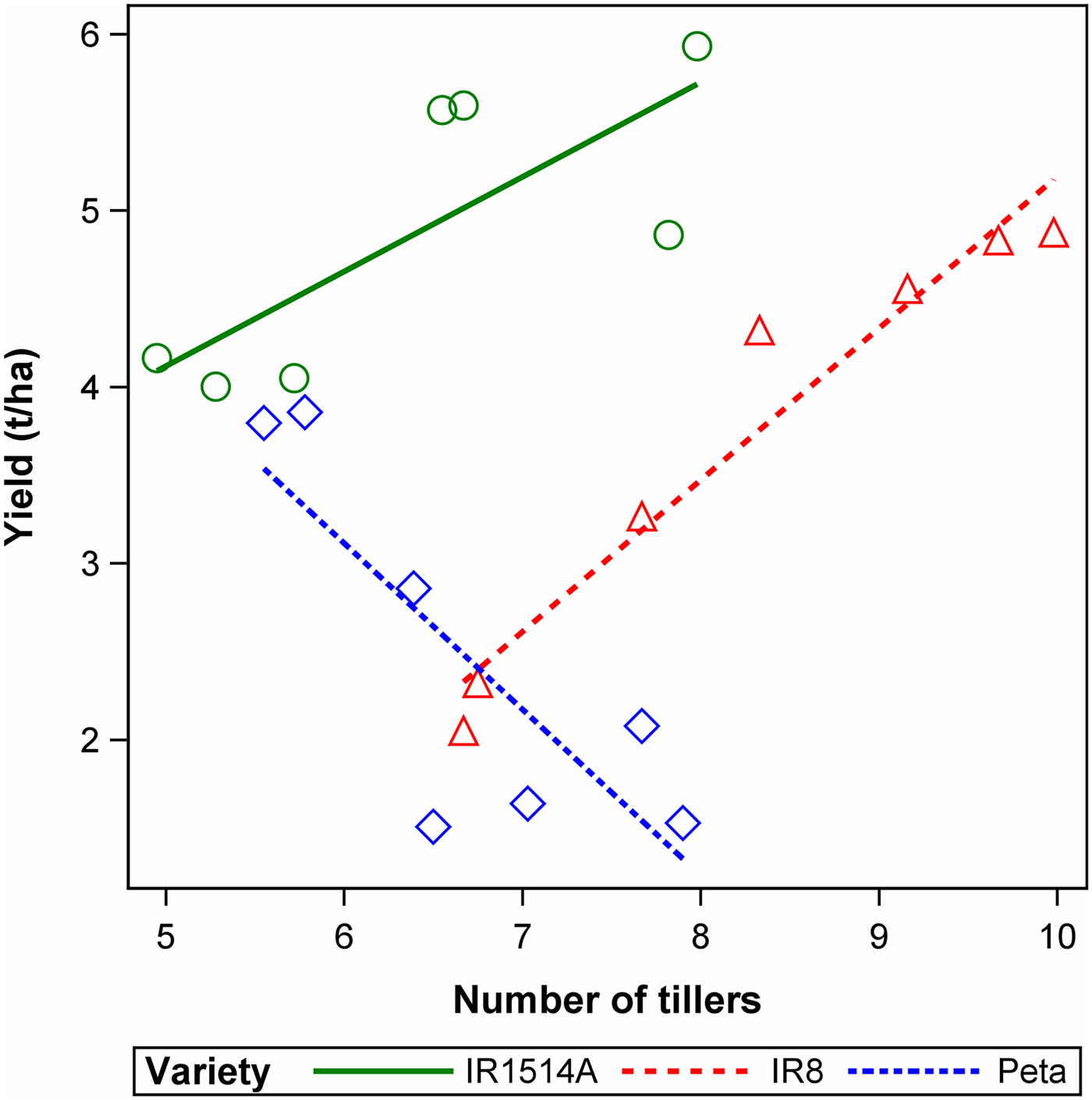
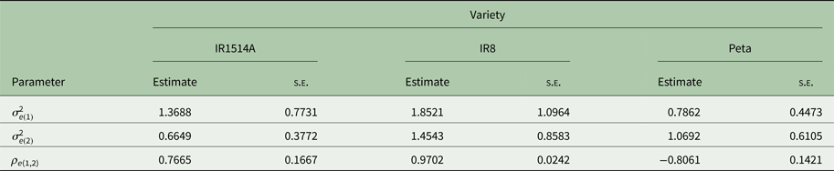
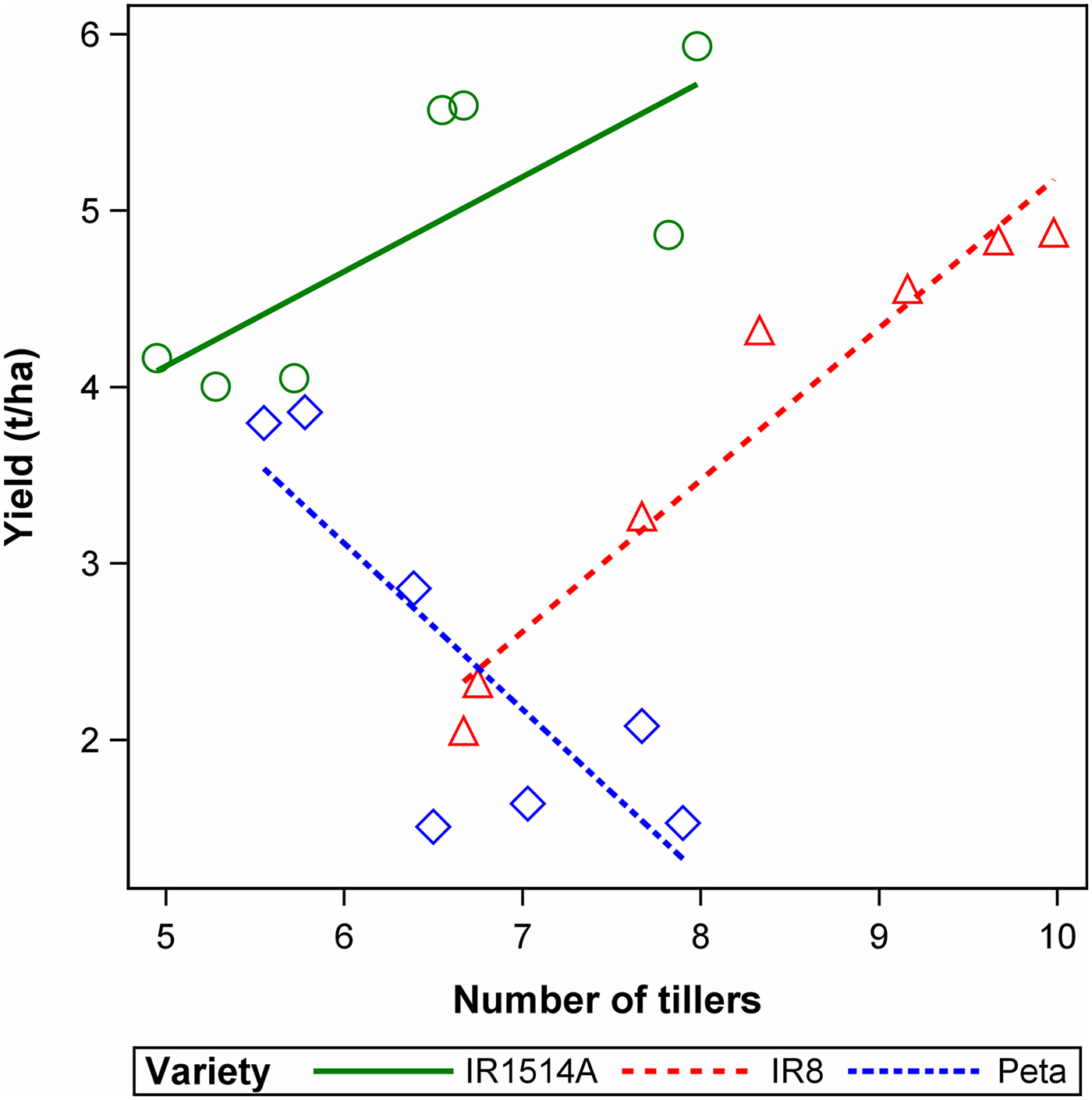
In an experiment with three rice cultivars (IR1514A, IR8 and Peta), the agronomic yield (t/ha) was assessed on seven plots per variety (Gomez & Gomez Reference Gomez and Gomez1984, p. 377, Table 9.4). On each plot, the number of tillers per hill was assessed. It is assumed here that the experiment was completely randomized, because Gomez & Gomez (Reference Gomez and Gomez1984) provide no information on any blocks in their table with the raw data, so our basic model is the one-way model in Eqn (1). Inspection of residuals for both traits indicated that approximate normality could be assumed. The sample correlation between the two traits is r = 0.1973 (P = 0.3912). Figure 9 shows a plot of yield versus the number of tillers, along with fitted regression lines per variety for emphasis of the general pattern. Obviously, there are strong correlations for the individual varieties, so the simple correlation ignoring the factor variety is grossly misleading. Moreover, Fig. 9 suggests that residual correlations differ markedly between varieties, meaning that the bivariate mixed model needs to allow for heterogeneity of residual variances and correlations. Heterogeneity of variance for a random effect is straightforward to implement in a mixed model. For example, in SAS one may use the option GROUP = variety on the REPEATED statement in order to allow the error variance to differ between varieties. Allowing for heterogeneity, the correlation of treatment effects is estimated as
 $\hat \rho _{\tau (1,2)} = - 0.1631$
(s.e. = 0.7734). The fit of the error variance parameters of the heterogeneous model is shown in Table 6. None of the correlations are anywhere near the simple correlation of r = 0.1973. Correlations for the errors are large in absolute value and positive for varieties IR1514A and IR8, but negative for variety Peta. This heterogeneity is significant by an LRT with a chi-squared value of T = 26.73 on 6 d.f. (P < 0.001). Due to the significant heterogeneity, and because correlations for errors are rather different from the correlation between treatment effects, it would be inappropriate here to compute a single marginal correlation for the observed data. This is also clear from graphical inspection of the scatter of points in Fig. 9. Instead, it seems more reasonable to focus on the treatment-specific residual correlations shown in Table 5 or fit variety-specific regression lines as shown in Fig. 3 (Gomez & Gomez Reference Gomez and Gomez1984). In fact, this ‘regression with groups’ with groups corresponding to varieties may be more informative for this dataset, but that analysis will not be explored in detail because our focus is on correlation. It is stressed, however, that correlation and regression analysis have close links. Specifically, a regression model can be derived from a bivariate mixed model by conditioning on one of the variates (Searle et al.
Reference Searle, Casella and McCulloch1992, p. 464). In the example, the slope for the regression of yield of a variety of tiller number can be derived as the ratio of covariance between the two traits over the variance of tiller number for that variety. It should also be pointed out that in general estimating correlation for an effect requires a reasonable number of levels for that effect. Three effects of treatments in this example are clearly a rather small number to make any substantive statement about correlation. This is why the focus was on the within-variety correlation.
Plot of yield (t/ha) v. number of tillers for rice (Oryza sativa L.) data for three varieties of rice, along with fitted regression lines for each variety (Gomez & Gomez Reference Gomez and Gomez1984, p. 377) (Example 3). Colour online.
Residual variance parameter estimates by variety for rice (Oryza sativa L.) data of Gomez & Gomez (Reference Gomez and Gomez1984, p. 377) (Example 3) under a model with heterogeneity between varieties
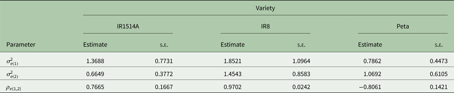
Trait 1 = number of tillers, trait 2 = yield of rice (t/ha).
Example 4
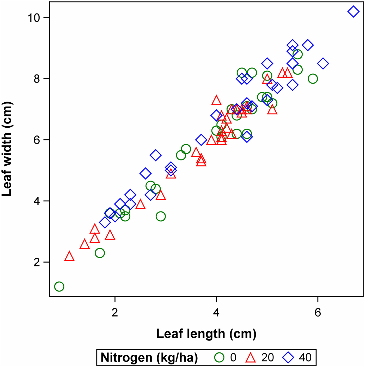
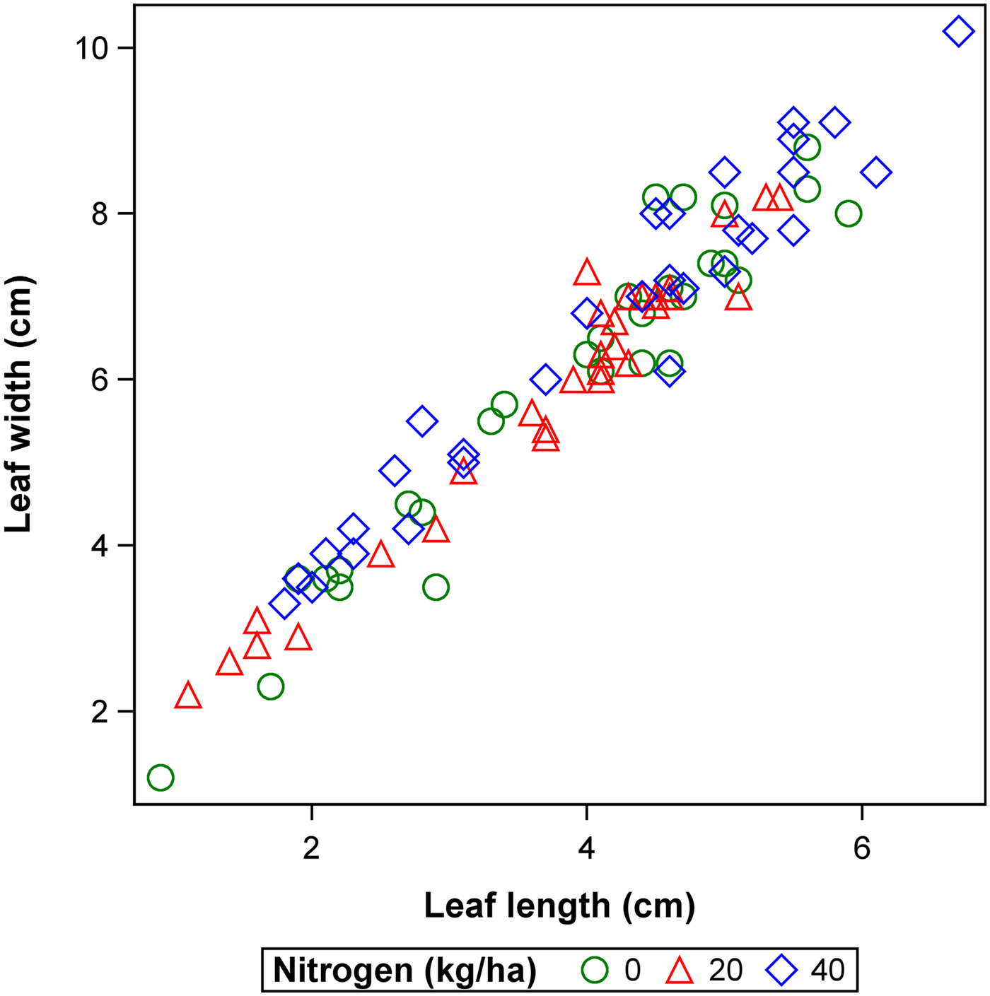
An experiment with chia (Salvia hispanica L.), laid out according to a randomized complete block design (RCBD), was performed in order to derive a prediction model for leaf area as a function of leaf width (cm) and leaf length (cm) (Mack et al. Reference Mack, Capezzone, Munz, Piepho, Claupein, Phillips and Graeff-Hönninger2017). The experiment comprised three nitrogen fertilizer treatments (0, 20 and 40 kg N/ha). On each plot, one chia plant was selected randomly and ten leaves were sampled per plant. For each leaf, the length, width and area were measured. The objective of the experiment was to identify a suitable prediction model for leaf area for individual leaves. As a preliminary step, it was therefore of interest to estimate the marginal correlation between leaf width and leaf length. The Pearson correlation between these two traits is r = 0.9697. The raw data are plotted in Fig. 10.
Scatter plot of leaf length (cm) v. leaf width (cm) for chia (Salvia hispanica L.) leaves from an RCBD experiment with three nitrogen treatments (0, 20 and 40 kg N/ha) (Mack et al. Reference Mack, Capezzone, Munz, Piepho, Claupein, Phillips and Graeff-Hönninger2017) (Example 4). Colour online.
Since there are subsamples (leaves) taken per plot, the linear model needs to be extended to comprise both a plot error as well as a leaf error. For a single trait, the model is:
 $$y_{ijk} = \mu + b_j + \tau _i + e_{ij} + f_{ijk} $$
where y
ijk
is the response of the kth leaf for ith treatment in the jth block, μ is a general intercept, b
j
is the effect of the jth block, τ
i
is the effect of the ith treatment, and e
ij
is the error term associated with the ijth plot, and f
ijk
is the residual leaf error associated with the response y
ijk
. This univariate model is extended to the bivariate model for leaf length and leaf width. Fitting this model, the block variance for leaf length was estimated to be zero (results not shown), and the statistical package reported a message indicating that the final Hessian was not positive definite. This reflects the fact that a correlation cannot be computed if one of the associated variances is zero. Thus, the random block effect for leaf length was dropped from the model. This was implemented by defining a dummy variable z with z = 0 for leaf length and z = 1 for leaf width. In coding the model using the statistical package, a block effect was then multiplied with this variable, such that the effect was ‘switched off’ for leaf length (Piepho et al.
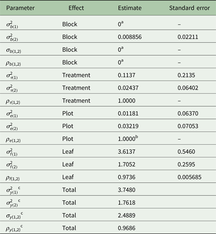
Reference Piepho, Williams and Fleck2006). The fitted model parameters for the bivariate model and the corresponding model under the null hypothesis that all effects are uncorrelated is shown in Table 7. The treatment and plot effects have an estimated correlation of 1.000, whereas the leaf effects have a correlation of
 $\hat \rho _{f(1,2)} = 0.9736$
. These very high correlations also translate into a very large marginal correlation of
 $\hat \rho _{y(1,2)} = 0.9686$
, again a meaningful summary in this case because effect correlations are so similar. The leaf effect correlation is highly significant (T = 248.73, P < 0.001), whereas the correlations for plot effects are not significant (T = 1.21, P = 0.2713). Also, the variances for leaf effects are rather larger than those for treatment and plot effects. Thus, the variance and covariance of leaf effects dominate the corresponding marginal variance and covariance for the observed data. This is also why the leaf error correlation, as well as the marginal correlation, are both rather close to the sample correlation of r = 0.9697. But whether a large sample correlation is also associated with large correlations of all the effects can only be verified by fitting a bivariate model as illustrated here.
Variance parameter estimates for chia (Salvia hispanica L.) data (Mack et al. Reference Mack, Capezzone, Munz, Piepho, Claupein, Phillips and Graeff-Hönninger2017) (Example 4) under the hypotheses H A : ρ y(1,2) ≠ 0
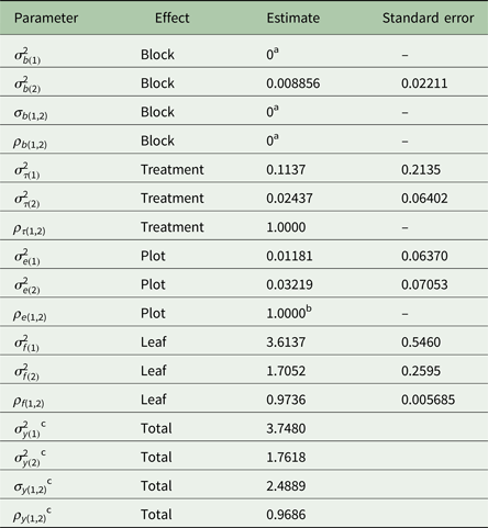
Trait 1 = leaf length (cm), trait 2 = leaf width (cm).
a Fixed at zero at convergence.
b Fixed at unity at convergence.
c These values were read off the output of the statistical package and are slightly different from the values one would obtain by plugging the estimates of variances and covariances for the effects shown in this table, which are rounded to the forth decimal place, into Eqns (26) to (28) for the marginal variances, covariance and correlation.
Concluding remarks
The present paper has considered the question of how to estimate and test correlations among traits in designed experiments. The common practice of merely computing sample correlations from the raw data should be discouraged because such correlations do not account for effects due to treatments and blocks and hence are difficult to interpret and the significance test for these correlations is invalid. The advice given in the current paper, therefore, is that the simple correlation not been used at all when the data have structure, as is the case in designed experiments. The main recommendation here is to use methods that allow accounting for all effects one would consider in a univarate analysis of a single trait, thus making the univariate and bivariate analyses commensurate. If one is primarily interested in correlations, then fitting a bivariate mixed model is suggested as a viable option. The approach allows decomposing correlation according to effects in the model, providing detailed insight into the structure of correlation. If the effects display a correlation of about equal magnitudes, then a marginal correlation accounting for these effects is a meaningful summary measure.
The first step of the analysis is to inspect the correlations for each of the effects of the bivariate model. This can be done using REML estimates of the correlations and use scatter plots of BLUPs of effects and residuals as illustrated with Examples 1 and 2. If correlations of effects are judged to be similar, either based on a non-significant LRT or from graphical inspection of scatter plots, the marginal correlation provides a meaningful summary of the data. Example 4 provides a case where the marginal correlation is the primary focus because good predictions are sought for leaf area at the level of individual observations. If the marginal correlation is high, which was the case here, one may fit a regression model for prediction (Mack et al. Reference Mack, Capezzone, Munz, Piepho, Claupein, Phillips and Graeff-Hönninger2017). Conversely, when correlations are deemed to be substantially heterogeneous between effects, it is necessary to study correlations at the level of individual effects. Most of the time, the research will mainly be interested in the treatment effects. Example 2 provides a pertinent example, where treatments correspond to genotypes and genetic correlation is a key quantitative genetic parameter. In Example 3, by contrast, there was heterogeneity of within-treatment correlation, so the study of the within-treatment error correlations proved to be most interesting. So, which of the effects is of primary interest in case of heterogeneity of correlations between effects needs to be decided on a case-by-case basis.
The proposed approach entails modelling block and treatment effects as random for the purpose of estimating correlations for these effects. If one is prepared to estimate a correlation for an effect, then the assumption of random effects will seem quite natural. Indeed, without assuming random effects, the notion of a correlation or covariance for effects, or of observations composed of these effects, may seem difficult to envisage. Yet, the choice of both treatments and blocks in a designed experiment may be such that the assumption of a random sampling of effects is deemed hard to justify. For this reason, one may insist that these effects should be modelled as fixed (Dixon Reference Dixon2016). It was shown for the case of a CRD, however, that variances and covariance for treatment effects can be defined also for fixed effects and that estimates of variances and covariances coincide under the fixed and random-effects assumptions. This equivalence holds more generally, as pointed out by Gelman (Reference Gelman2005, p. 13), who denotes a fixed-effects variance such as Q(τ) in (14) as finite-population variance, and the random-effects equivalent such as
 $\sigma _\tau ^2 $
as superpopulation variance. This fact lends support to the approach proposed here, i.e. to take effects as random for the purpose of estimating correlations, even in settings where one would otherwise hesitate to model block and treatment effects as random. There is, of course, a long-standing debate in the statistical literature as to whether blocks should be modelled as fixed or random. This is not the place to review that debate, but it should be pointed out that one camp insists that block effects should always be modelled as random, even for an RCBD (Nelder Reference Nelder1965; Casella & Berger Reference Casella and Berger1990, p. 530; Giesbrecht & Gumpertz Reference Giesbrecht and Gumpertz2004, p. 86; Booth et al.
Reference Booth, Federer, Wells and Wolfinger2009). The assumption of random treatment effects is less common, except in breeding experiments where treatments correspond to genotypes which can be regarded as a (usually large) sample from a common breeding population and the main interest is in making inferences about that population, including estimation of genetic correlation between traits, heritability of traits, etc. (Falconer & Mackay Reference Falconer and Mackay1996). But note that even with a relatively small number of levels of an effect and lacking truly random sampling, the random assumption can be beneficial for inference about a treatment effect (James & Stein Reference James, Stein and Neyman1961; Lee et al.
Reference Lee, Nelder and Pawitan2006, p. 151; Forkman & Piepho Reference Forkman and Piepho2013). Certainly, if a Bayesian framework is adopted, there is no conceptual difficulty in assuming a joint probability distribution on all unknown parameters, including effects for treatments (Gelman Reference Gelman2005).
The bivariate model used in the current paper has been considered by Booth et al. (Reference Booth, Federer, Wells and Wolfinger2009), who used it to derive an analysis-of-covariance model by conditioning on the observed values of one of the traits, regarded as the concomitant variable (covariate). The definition of the marginal correlation in (25) is not entirely novel either. It is very similar to the one proposed by Hill & Thompson (Reference Hill and Thompson1978; also see Singh & El-Bizri Reference Singh and El-Bizri1992), also for an RCBD, for the specific context of genetic experiments where treatments correspond to genotypes. The difference is that for a blocked design the marginal correlation in (25) includes the block effects, while Hill & Thompson (Reference Hill and Thompson1978) exclude the block effect from the definition of marginal correlation because it is irrelevant for selection decisions. Depending on the objective one may decide to either include or omit the block effect from the correlation. The same holds for any other design, where one needs to decide if design effects for blocks should be included in the definition of total correlation. The great advantage of the REML framework employed here is its generality and complete flexibility in terms of the effects that are included in the overall model and in the definition of total correlation. In plant breeding and quantitative genetic experiments, where the focus is on genetic correlation, block effects are not relevant in the definition of marginal correlations, but they need to be fitted nonetheless to represent the experimental design (Piepho & Möhring Reference Piepho and Möhring2011).
Before fitting a bivariate random-effects model, it is advisable to fit univariate random-effects models to the individual traits. If a variance for an effect is estimated to be zero for at least one of the traits, a covariance cannot be fitted, because a covariance requires both variances to be non-zero and a correlation cannot be defined otherwise. It is then reasonable to constrain the bivariate model to have a zero covariance for such effects. If the variance of an effect is zero for only one trait, however, it needs to be kept in the model, but the covariance explicitly constrained to be zero. Most mixed models have covariance structures for this case, known as ‘diagonal model’ in some packages. In SAS, the structure is denoted as UN(1). Alternatively, one can use dummy coding as illustrated with Example 4. Diagonal covariance structures can also be used to fit two univariate models simultaneously as a joint bivariate model assuming independence for all effects.
The proposed methods were illustrated using experiments laid out according to a CRD, an RCBD (with sub-sampling per plot) or a lattice design, but the framework is broadly applicable to any experimental design. All that needs to be done is taking each effect of the bivariate model as random, assuming a bivariate normal distribution. Multivariate linear mixed models can also be fitted to more than two traits simultaneously and when data are unbalanced (Holland Reference Holland2006; Piepho & Möhring Reference Piepho and Möhring2011) or when spatial covariance needs to be modelled (Ganesalingam et al. Reference Ganesalingam, Smith, Beeck, Cowling, Thompson and Cullis2013; de Faveri et al. Reference De Faveri, Verbyla, Cullis, Pitchford and Thompson2017), but occasionally convergence problems may hamper such analyses. Good starting values are crucial to larger problems. One option to obtain starting values for the variances is to fit univariate models separately for each trait. Covariances can be obtained from univariate analyses of differences or sums of two traits (see Eqn (22) and accompanying text; Searle et al. Reference Searle, Casella and McCulloch1992; Piepho et al. Reference Piepho, Müller and Jansen2014).
The present paper has focused on correlation in bivariate data, stressing the importance of accounting for effects of blocks and treatments. This is also important when regression is used instead of correlation, which may be more informative. Figure 3 for Example 3 shows fitted regression lines for each variety, providing variety-specific predictions of yield as a function of tiller numbers. The regression lines very clearly show that the associations between yield and tiller number are rather different between varieties. In this example, fitting a single regression line through all points, ignoring the varieties, obviously makes as little sense as computing a simple correlation coefficient. If the regressor variable shows no treatment effect and slopes are identical across treatments, regression analysis accounting for block and treatment effects in the response is known as analysis of covariance (Milliken & Johnson Reference Milliken and Johnson2002; Pearce Reference Pearce, Kotz, Balakrishnan, Read and Vidakovic2006). When there is an interaction between treatment and covariate, i.e. slopes differ between treatments as is the case in Example 3, a regression with groups is appropriate.
Supplementary material
The supplementary material for this article can be found at https://doi.org/10.1017/S0021859618000059.
Acknowledgements
I sincerely thank Philip Dixon (Department of Statistics, Iowa State University) for providing a preprint of his interesting article and for very inspiring discussions on the modelling of block effects in designed experiments during my visit at Iowa State University, which eventually prompted me to finally sit down and write this paper, which I had wanted to write for a long time. Berhard Ludwig (Universität Kassel) is thanked for very helpful comments on an earlier version of the paper. Further, I wish to thank Friedrich Utz (University of Hohenheim) for providing the oats data used in Example 2. Thanks are also due to Laura Mack of the Anton & Petra Research Ehrmann-Stiftung Research Training group ‘Water – People –Agriculture’ at the University of Hohenheim (Germany) for providing the Chia trial data, and to the team at Ihinger Hof (University of Hohenheim, Germany) for invaluable technical support in conducting the trial. The German Research Foundation (DFG) is thanked for financial support (grant PI 377/18-1). Last but not least, I thank the reviewer for very helpful and constructive comments.