

The differential-susceptibility hypothesis, which stipulates that some individuals are more susceptible than others to both positive and negative environmental effects, perhaps most especially parenting, has received substantial attention and empirical support in recent years (Belsky, Bakermans-Kranenburg, & van IJzendoorn, Reference Belsky, Bakermans-Kranenburg and van IJzendoorn2007; Belsky & Pluess, Reference Belsky and Pluess2013; Ellis, Boyce, Belsky, Bakermans-Kranenburg, & van IJzendoorn, Reference Bakermans-Kranenburg and van IJzendoorn2011; Pluess & Belsky, Reference Pluess and Belsky2009, Reference Pluess and Belsky2010), including in research on Gene × Environment (G × E) interaction (Bakermans-Kranenburg & van IJzendoorn, Reference Bakermans-Kranenburg and van IJzendoorn2011; Belsky et al., Reference Belsky, Jonassaint, Pluess, Stanton, Brummett and Williams2009; Belsky & Pluess, Reference Belsky and Pluess2009; Berry, Deater-Deckard, McCartney, Wang, & Petrill, Reference Berry, Deater-Deckard, McCartney, Wang and Petrill2013). Here we test the specific proposition that a set of 12 candidate “plasticity genes,” selected principally on the basis of prior reviews of relevant research (Belsky et al., Reference Belsky, Jonassaint, Pluess, Stanton, Brummett and Williams2009; Belsky & Pluess, Reference Belsky and Pluess2009), will moderate the effects of maternal sensitivity on children's social–emotional and cognitive–linguistic development in a manner consistent with the differential-susceptibility hypothesis. Toward this end, we employ two new statistical methods, applying them to longitudinal data collected from the National Institute of Child Health and Human Development Study of Early Child Care and Youth Development (NICHD SECCYD; NICHD Early Child Care Research Network [ECCRN], 2005), in response to questions raised about the adequacy and appropriateness of existing statistical criteria for evaluating differential susceptibility (Belsky, Pluess, & Widaman, Reference Belsky, Pluess and Widaman2013; Roisman et al., Reference Roisman, Newman, Fraley, Haltigan, Groh and Haydon2012; Widaman et al., Reference Widaman, Helm, Castro-Schilo, Pluess, Stallings and Belsky2012). The application of appropriate analytic criteria for differential susceptibility is necessary to minimize Type 1 errors and failures to replicate that have frustrated previous work on candidate genes and broad phenotypes of human cognition, personality, and social behavior (Charney & English, Reference Charney and English2012; Deary, Reference Deary2012; Wacker, Mueller, Hennig, & Stemmler, Reference Wacker, Mueller, Hennig and Stemmler2012).
Theories of Socialization and Maternal Sensitivity
A central assumption of many developmental perspectives on socialization, whether based, for example, on theories of attachment (Ainsworth, Reference Ainsworth, Caldwell and Ricciuti1973; Sroufe, Reference Sroufe2000), social learning (Patterson, Reference Patterson1986), or evolution (Belsky, Steinberg, & Draper, Reference Belsky, Steinberg and Draper1991), is that parenting matters when it comes to how children develop. Although a myriad of parenting constructs are measured in socialization research, including, for example, authoritative parenting (Baumrind, Reference Baumrind1967, Reference Baumrind1991), coercive parenting (Patterson, Reference Patterson1986), and mutually responsive relationships (Kochanska, Reference Kochanska2002), the focus in the present report is on sensitive parenting, a construct emphasized in attachment theory. According to Ainsworth (1969), sensitive parenting involves reading the child's cues accurately and responding in a timely and appropriate fashion. However, this conceptualization has been operationalized in a number of ways, perhaps most clearly chronicled in De Wolf and van IJzendoorn's (Reference De Wolff and van IJzendoorn1997) meta-analysis of the effects of sensitivity on attachment security, where diverse measures of warmth, responsiveness, expressions of positive affect, and interactional synchrony all proved to function similarly when it came to predicting attachment security.
Early sensitivity is not only clearly and causally related to the development of attachment security (for meta-analysis, see Bakermans-Kranenburg, van IJzendoorn, & Juffer, Reference Bakermans-Kranenburg, van IJzendoorn and Juffer2003) but also predicts a diverse array of developmental outcomes (e.g., Jaafari-Bimmel, Juffer, van IJzendoorn, Bakermans-Kranenburg, & Mooijaart, Reference Jaffari-Bimmel, Juffer, van IJzendoorn, Bakermans-Kranenburg and Mooijaart2006; Sroufe, Egeland, Carlson, & Collins, Reference Sroufe, Egeland, Carlson and Collins2005). In the NICHD SECCYD, for example, a composite measure of sensitivity averaged across the early childhood years proved consistently predictive of virtually every developmental outcome investigated, whether socioemotional or cognitive–linguistic in character, and more so than any measure of childcare experience (Belsky et al., Reference Belsky, Bakermans-Kranenburg and van IJzendoorn2007; Fraley, Roisman, & Haltigan, Reference Fraley, Roisman and Haltigan2013; Haltigan, Roisman, & Fraley, Reference Haltigan, Roisman and Fraley2013; NICHD ECCRN, 2006; Vandell et al., Reference Vandell, Belsky, Burchinal, Steinberg and Vandergrift2010). This program of research was not genetically informed and thus not positioned to discount or illuminate the possible genetic basis of the presumptive environmental effects chronicled (but see Roisman & Fraley, Reference Roisman and Fraley2012). The same limitation should be acknowledged with regard to the research reported here.
Central to most theories of socialization (whether they emphasize sensitive-responsiveness, coercive dyadic exchanges, authoritative parenting, or mutually reciprocal relationships) is the implicit if not explicit assumption that most if not all children are susceptible to the developmental benefits of supportive rearing and/or the adverse consequences of unsupportive parenting. For example, Baumrind's (Reference Baumrind1967) theory of parenting does not presume that some children reap the rewards of authoritative parenting more than others; and the same is true of Patterson's (Reference Patterson1982) view of the antisocial consequences of coercive parenting that inadvertently rewards children's angry, disputatious behavior. Nor is it the case that Ainsworth (Reference Ainsworth, Caldwell and Ricciuti1973) theorized that sensitive parenting would foster secure attachment in only some children and not others or more so in some than others. Belsky et al. (Reference Belsky, Steinberg and Draper1991) raised this possibility in advancing their evolutionary theory of socialization, but only in passing.
The Diathesis–Stress Framework
The notion that individuals differ in their susceptibility to environmental effects has a long history in psychiatry and psychology (Belsky & Pluess, Reference Belsky and Pluess2009). Sameroff's (Reference Sameroff and Mussen1983) transactional model of development raised the possibility that, for example, certain children already at risk for developmental difficulties for organismic reasons (e.g., premature birth) would be especially likely to be adversely affected by contextual sources of development risk, including problematic parenting. Furthermore, this view has been central to a large body of work on Temperament × Parenting interactions (for a review, see Rothbart & Bates, Reference Rothbart, Bates, Eisenberg, Damon and Lerner2006) and psychopathology (Gottesman & Shields, Reference Gottesman and Shields1967; Zuckerman, Reference Zuckerman1999). Implicitly or explicitly, the diathesis–stress conceptual framework has guided much developmental and clinical inquiry.
Central to the diathesis–stress framework is the view that certain individuals are especially vulnerable to contextual adversity (e.g., problematic parenting) as a result of endogenous characteristics (Gottesman & Shields, Reference Gottesman and Shields1967; Zuckerman, Reference Zuckerman1999), most notably, genetic makeup, the focus of this report. Diathesis–stress thinking spawned some of the first G × E interaction research examining the co-action of putative “vulnerability genes” or “risk alleles” and child maltreatment in predicting young adults' antisocial behavior (Caspi et al., Reference Caspi, McClay, Moffitt, Mill, Martin and Craig2002). As another example, diathesis–stress thinking also yielded predictions that prenatal smoking would result in elevated attention-deficit/hyperactivity disorder symptoms when children carried a particular risk allele, the 7 repeat of the dopamine receptor D4 polymorphism (DRD4; Neuman et al., Reference Neuman, Lobos, Reich, Henderson, Sun and Todd2007), as it did.
The Differential-Susceptibility Framework
What was not apparently entertained in the first wave of human G × E research or in developmental research on socialization was that some individuals would not just prove more susceptible to the developmental costs of unsupportive rearing (or other forms of contextual adversity), but that the same putatively “vulnerable” individuals would be especially likely to reap the developmental benefits of supportive parenting (or other forms of contextual support). Yet this is exactly what the differential-susceptibility hypothesis predicts: individual differences in developmental plasticity (Belsky, Reference Belsky1997, Reference Belsky, Ellis and Bjorklund2005; Belsky et al., Reference Belsky, Bakermans-Kranenburg and van IJzendoorn2007, 2010; Belsky & Pluess, Reference Belsky and Pluess2009, Reference Belsky and Pluess2013; Ellis et al., Reference Ellis, Boyce, Belsky, Bakermans-Kranenburg and van IJzdenoorn2011). That is, some children will be more affected by their parenting experiences than others, for better and for worse (Belsky et al., Reference Belsky, Bakermans-Kranenburg and van IJzendoorn2007), as a result of their own temperamental, physiological, and/or genetic makeup, although it is the latter that is of central concern to this report. This evolutionary perspective on parenting effects (and other environmental experiences and exposures) was founded on the view that, because the future is inherently uncertain, parents' and children's inclusive fitness would not be optimized if every child were equally developmentally malleable or plastic.
The logic of this view is that regulating future functioning based on developmental experiences would pay off principally when the future was tolerably consistent with the past, but this would not be the case when the world the child came to live in as she or he grew up diverged markedly from that of childhood (Belsky, Reference Belsky1997, Reference Belsky, Ellis and Bjorklund2005; Ellis et al., Reference Ellis, Boyce, Belsky, Bakermans-Kranenburg and van IJzdenoorn2011). In other words, differential susceptibility to rearing (and other environmental experiences and exposures) could function as a means by which children and parents hedged their inclusive-fitness bets. The biologic here is exactly the same as that which recommends diversification of economic investments. Because one can never know whether an investment offering a fixed and predictable return will lose value over time due to inflation exceeding that figure, and because one can never know whether a particular equity's value will increase or decrease over time, portfolio theory stipulates hedging bets by not putting all eggs in one basket.
There is a large body of recent evidence that seems to indicate that children vary in their susceptibility to rearing effects, and in a for better and for worse manner, and that this is so whether one considers temperamental, physiological, or genetic factors as moderators of environmental effects and thus markers of greater and lesser developmental plasticity (for reviews, see Belsky, Reference Belsky, Ellis and Bjorklund2005; Belsky & Pluess, Reference Belsky and Pluess2009, Reference Belsky and Pluess2013; Obradović & Boyce, Reference Obradović and Boyce2009; Pluess & Belsky, Reference Pluess and Belsky2009, Reference Pluess and Belsky2010). That this appears to be the case for some polymorphisms long regarded as “vulnerability genes” or “risk alleles” served as the impetus for the proposal that they be reconceptualized as “plasticity genes” (Belsky et al., Reference Belsky, Jonassaint, Pluess, Stanton, Brummett and Williams2009). Consider in this regard the following very recent and illustrative findings pertaining to the genetic moderation of parenting effects by each of 3 (of 12) putative plasticity genes examined in the current report:
1. Hankin et al. (Reference Hankin, Jenness, Abela and Smolen2011) observed that positive parenting was more strongly associated with the positive affect of 8- to 12-year-olds (in a for better and for worse fashion) in the case of children carrying short alleles on the serotonin transporter linked polymorphic region gene (5-HTTLPR) than for those carrying other versions of this gene.
2. Knafo, Israel, and Ebstein (Reference Knafo, Israel and Ebstein2011) reported that mother's failure to explain her reasons for punishing the child predicted preschoolers' observed prosocial behavior, again in a differential-susceptibility related manner, and thus only in the case of those carrying the DRD4 7-repeat allele.
3. Finally, Suzuki et al. (Reference Suzuki, Matsumoto, Shibuya, Sadahiro, Kamata and Goto2011) found that retrospectively reported parental rearing predicted the personality trait of self-directedness more strongly in those homozygous for the methionine allele on the brain-derived neurotrophic factor Val66Met polymorphism (BDNF) than those homozygous for the valine allele, such that the former scored highest and lowest on self-directedness as a function of whether they experienced more and less supportive rearing, respectively.
Despite such evidence for plasticity genes, questions can be raised about the interpretation of findings (Roisman et al., Reference Roisman, Newman, Fraley, Haltigan, Groh and Haydon2012). When Belsky (Reference Belsky, Ellis and Bjorklund2005) first reviewed evidence on temperament (and later physiology) and G × E interaction that routinely had been interpreted in diathesis–stress terms but appeared to reflect differential susceptibility (Belsky et al., Reference Belsky, Jonassaint, Pluess, Stanton, Brummett and Williams2009; Belsky & Pluess, Reference Belsky and Pluess2009), he and his associates relied on a very simple method of evaluation: visual inspection of graphic displays of crossover interactions reflecting environmental factor and moderator in predicting some phenotypic measurement. Thus, a liberal criterion was established to raise the prospect of differential susceptibility; more specifically, the predictor–outcome relation had to be stronger and graphically steeper in one subgroup than another once a significant statistical interaction was decomposed.
In attempt to refine the evaluation of differential susceptibility, Belsky et al. (Reference Belsky, Bakermans-Kranenburg and van IJzendoorn2007) delineated more specific and demanding statistical criteria. In addition to the detection of a significant crossover interaction between the environmental predictor (e.g., parenting) and the plasticity or moderating factor (e.g., candidate gene), also required was evidence that the slope reflecting the predictor–outcome association be significant in the case of one subset of research participants but not the other or that the slope of the former be significantly greater than that of the latter. Two independent teams (Belsky et al., Reference Belsky, Pluess and Widaman2013; Roisman et al., Reference Roisman, Newman, Fraley, Haltigan, Groh and Haydon2012; Widaman et al., Reference Widaman, Helm, Castro-Schilo, Pluess, Stallings and Belsky2012) recently offered even more exacting criteria that must be met for a conclusion of differential susceptibility to be embraced. Each is discussed in turn, because each will be employed in the research reported herein when testing the proposition that children carrying specific alleles of candidate genetic plasticity markers will be more susceptible than others to sensitive and insensitive parenting.
The Roisman and Colleagues Approach
Roisman et al. (Reference Roisman, Newman, Fraley, Haltigan, Groh and Haydon2012) proposed a set of recommendations to overcome four limitations of existing methods used to evaluate differential susceptibility. One recommendation is that investigators conduct regions of significance (RoS) tests to determine the full range of values of the moderator for which the regression of the outcome on the predictor (X) is statistically significant. Although these tests, first used by Kochanska, Kim, Barry, and Philibert (Reference Kochanska, Kim, Barry and Philibert2011) in relation to the differential susceptibility hypothesis, can be employed to examine the values of the moderator (M) for which the association between X and Y is significant, these tests can also be used to examine the values of the predictor for which the association between M and Y is significant.
Roisman et al. (Reference Roisman, Newman, Fraley, Haltigan, Groh and Haydon2012) recommend that the difference between those with and without (or high vs. low on) the moderator should be significant both on the low end of X and on the high end of X before concluding that results are consistent with differential-susceptibility predictions. Because the difference can be significant at values of X that are not represented in the sample (e.g., at 14 SD below the mean), Roisman et al. further recommended that investigators conduct RoS tests using common regions of interest (i.e., the range of X for the RoS on X test should be bounded by ±2 SD).
The second recommendation by Roisman et al. (Reference Roisman, Newman, Fraley, Haltigan, Groh and Haydon2012) is to use new metrics specifically designed to index disordinal-interaction effects. Roisman et al. proposed two closely related indices that take advantage of the crossover point of the interaction providing a natural way to conceptualize the point at which an effect of Z on Y can change from “for better” to “for worse.” The first metric, labeled the proportion of interaction (PoI) index, represents the proportion of the total area between the lines of an interaction plot, bounded by ±2 SD on X, that is above the crossover point. In a prototypical interaction plot for differential susceptibility, the lines will cross over near the mean of X; as a result, 50% of the area bounded by the regression lines in such a plot would represent the for better region. In a prototypical case of diathesis–stress (i.e., an ordinal interaction), the crossover point will be on the far right side of the plot and 0% of the total area will represent the for better region.
The second index, labeled the proportion affected or the percentage above (PA) index, is similar to the PoI, but it is designed to quantify the proportion of all people in the sample who fall above the crossover point for the interaction. This value is an estimate of the number of people in the sample who are differentially affected “for the better.” In a prototypical differential susceptibility situation, 50% of people will be differentially affected for the better by Z (e.g., difficult temperament) as a function of X (e.g., parenting). In a prototypical diathesis–stress situation, 0% of people will be differentially affected for the better by Z as a function of X. When used in this manner, Roisman et al. (Reference Roisman, Newman, Fraley, Haltigan, Groh and Haydon2012) recommend that differential susceptibility is highly consistent with PoI values between 40% and 60%, or PA values equal to or greater than 16%.
The third recommendation involves testing for nonlinearity; thus, before investigators conclude in favor of differential susceptibility, they first demonstrate that neither X 2, ZX 2, nor the combination of X 2 and ZX 2 is statistically significant; and if one or more of these terms is significant, then a researcher must demonstrate that the interaction between X and Z holds when these nonlinear terms are statistically controlled. This can be useful because, if predictor X (e.g., maternal sensitivity) has a quadratic association with outcomes, but only when Z is low, it is possible to find evidence suggesting that some individuals experience beneficial effects of Z (e.g., difficult temperament) when they do not.
Roisman et al.'s (Reference Roisman and Fraley2012) fourth recommendation is that investigators attend to Type I error rates when examining multiple interactions in multiwave data sets. They thus offered two ways of solving this problem: use multilevel models to examine differential susceptibility across the entire developmental course under investigation (i.e., an intercepts as outcomes model) and adjust alpha when multiple comparisons are considered.
The Widaman and Colleagues Approach
In an independent contribution, Widaman et al. (Reference Widaman, Helm, Castro-Schilo, Pluess, Stallings and Belsky2012; Belsky et al., Reference Belsky, Pluess and Widaman2013) offered a model-comparison approach for evaluating whether interactions reflect differential susceptibility or diathesis–stress. In contrast to Roisman et al. (Reference Roisman, Newman, Fraley, Haltigan, Groh and Haydon2012), it does not require a statistically significant G × E interaction before proceeding to evaluate the form of the interaction, though formal statistical indices are used to select the best fitting model.
Under diathesis–stress theorizing, the predicted interaction should be ordinal in form. Consider a biallelic polymorphism with three possible genotypes, containing 0, 1, or 2 putative risk alleles. According to diathesis–stress, a regression model with a Linear G × Linear E interaction should reveal four outcomes: a small or zero effect of the environment for the (resilient) group with 0 risk alleles; a stronger, significant effect of the environment for the group with 2 risk alleles; a middling outcome by the group with 1 risk allele; and a crossover point of the linear functions at or near the most positive value for the environment.
Differential susceptibility leads to a contrasting prediction regarding the form of the G × E interaction. The alternate alleles under differential susceptibility are recast as plasticity and nonplasticity alleles, rather than risk and resilience alleles, respectively. The predicted interaction would still have a small (or nil) effect of the environment for the least-plastic group, a stronger, significant effect of the environment for the plastic group, and a moderate effect for the moderately plastic group. The crossover point of these three linear functions would be near the middle of the distribution of scores on the environmental variable, thus revealing a “for better and for worse” pattern (Belsky et al., Reference Belsky, Bakermans-Kranenburg and van IJzendoorn2007), with “better” outcomes (i.e., greater social competence) predicted for the most-plastic group under more favorable environmental conditions and “worse” outcomes (i.e., less social competence) for the most-plastic group under less favorable ones.
The location of the crossover point for the predicted outcomes is therefore the crucial parameter that distinguishes predictions for the G × E interaction for the competing diathesis–stress and differential-susceptibility positions. Widaman et al. (Reference Widaman, Helm, Castro-Schilo, Pluess, Stallings and Belsky2012) proposed a reparameterized regression model that makes the crossover point one of the parameters to be estimated. One major benefit of the reparameterization is that the point estimate of the crossover point is accompanied by a standard error, so that an interval estimate can be calculated. Among other things, the reparameterized model allows model fit under differential-susceptibility and diathesis–stress conditions to be statistically contrasted, with the better fitting model offered as the optimal representation of the data.
Widaman et al. (Reference Widaman, Helm, Castro-Schilo, Pluess, Stallings and Belsky2012; Belsky et al., Reference Belsky, Pluess and Widaman2013) highlighted four reparameterized models that can provide tests of key parameters consistent with (a) weak and (b) strong differential-susceptibility and (c) weak and (d) strong diathesis–stress predictions. Whereas strong models presume that some individuals are not at all susceptible to environmental effects (i.e., zero-order association between predictor and outcome), weak models presume that all are susceptible but that some are more so than others. As with the Roisman et al. (Reference Roisman, Newman, Fraley, Haltigan, Groh and Haydon2012) approach, Widaman et al. (Reference Widaman, Helm, Castro-Schilo, Pluess, Stallings and Belsky2012; Belsky et al., Reference Belsky, Pluess and Widaman2013) stressed that an initial screening should be done to discount the presence of nonlinearities in relations among variables in the model. By the same token, given the model-testing approach central to Widaman et al. (Reference Widaman, Helm, Castro-Schilo, Pluess, Stallings and Belsky2012; Belsky et al., Reference Belsky, Pluess and Widaman2013), only if the nature of the interactions being evaluated prove consistent with the a priori predictions on which the modeling is based would the fit of any model be regarded as meaningful and thus interpretable.
The Current Study
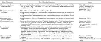
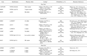
In the current study we employed both of the new statistical approaches just outlined for evaluating differential susceptibility. In particular, we used the six diagnostics for disordinal interactions (e.g., differential susceptibility) described in Table 1. The first four diagnostics and the crossover point reflect the Roisman et al. (Reference Roisman, Newman, Fraley, Haltigan, Groh and Haydon2012) approach, whereas the final two reflect the Widaman et al. (Reference Widaman, Helm, Castro-Schilo, Pluess, Stallings and Belsky2012) approach. We used these diagnostics to evaluate the proposition that maternal sensitivity/insensitivity, measured repeatedly across the opening years of life, differentially predicts, depending on the child's genotype, socioemotional and cognitive–linguistic functioning measured repeatedly from as early as age 24 months to as late as 15 years. More specifically, we focused on 12 candidate plasticity markers to determine whether they moderated the parenting/child-development associations under investigation in a for better and for worse, differential-susceptibility related manner. With two exceptions, the candidate plasticity markers selected for consideration are the ones to which Belsky and Pluess (Reference Belsky and Pluess2009) called attention in their review of G × E evidence seemingly consistent with differential susceptibility. Table 2 delineates the candidate plasticity genes that are the focus of inquiry, whether they were highlighted in the aforementioned review, and which alleles are expected to identify children who are more rather than less susceptible to the effects of maternal sensitivity in a differential-susceptibility related manner; listed in the table as well are some reports that chronicled differential susceptibility using the genes in question.
Six diagnostics for probing Gene × Environment interactions

Note: Per Roisman et al. (Reference Roisman, Newman, Fraley, Haltigan, Groh and Haydon2012), the first four diagnostics should be applied only after one detects a statistically significant interaction effect (i.e., H 0:B 3 = 0), using appropriate Type I error control; regression equation Ŷ i = b 0 + b 1X i + b 2Z i + b 3X iZ i. Diagnostic 5 relies on information indices, such as AIC and BIC, to identify the optimal model.
Plasticity genes

aBased on Belsky and Pluess (Reference Belsky and Pluess2009).
bPercentages may sum to greater than 100%, due to rounding.
cBased on emerging evidence since Belsky and Pluess (Reference Belsky and Pluess2009).
Because virtually all of these 12 genes are implicated in the functioning of the dopaminergic and/or serotonergic neurotransmitter systems in ways discussed and reviewed by Belsky and Pluess (Reference Belsky and Pluess2009), in the interests of space we do not consider here possible biological mechanisms by which these genes may come to moderate the parenting effects under investigation. This also seems reasonable because absolutely no mechanism-related measurements are included in this inquiry, meaning that any and all discussion of how the candidate plasticity genes under investigation might moderate the effects of parenting would be entirely speculative. The question we ask is simply whether genetic moderation in a manner consistent with differential susceptibility proves evident, not why this is the case mechanistically. Moreover, we appreciate that the candidate polymorphisms considered in this report are likely just markers for complex, multigenetic, and multilevel processes, so breathing “mechanistic meaning” into them risks implying that they are much more than proxies for complex biological processes that remain unmeasured (see Charney & English, Reference Charney and English2012).
Table 2 is organized to highlight three candidate genes we were most confident would moderate effects of maternal sensitivity in a differential-susceptibility related manner and nine others we were less confident about, divided into two subgroups for reasons articulated below. The three polymorphisms in the top tier are 5-HTTLPR, DRD4, and BDNF. Not only were the first two highlighted in the research reviewed by Belsky and Pluess (Reference Belsky and Pluess2009), but also multiple additional G × E studies have emerged since the preparation of that review indicating that these polymorphisms operate like plasticity genes (e.g., 5-HTTLPR; Brody et al., Reference Brody, Beach, Chen, Obasi, Philibert and Kogan2011; Carver, Johnson, Joorman, Kim, & Nam, Reference Carver, Johnson, Joormann, Kim and Nam2011; Hankin, Jenness, et al., Reference Hankin, Jenness, Abela and Smolen2011; Hankin, Nederohof, et al., Reference Hankin, Nederhof, Oppenheimer, Jenness, Young and Abela2011; Kuepper et al., Reference Kuepper, Wielpuetz, Alexander, Mueller, Grant and Hennig2012; DRD4: Fortuna et al., Reference Fortuna, van IJzendoorn, Mankuta, Kaitz, Avinun and Epstein2011; Knafo et al., Reference Knafo, Israel and Ebstein2011; Park, Sher, Todorov, & Heath, Reference Park, Sher, Todorov and Heath2011; Verschoor & Markus, Reference Verschoor and Markus2011). The same appears true of BDNF, a candidate gene that was not included in the Belsky and Pluess (Reference Belsky and Pluess2009) review, because it is only in the time since that review was prepared that G × E evidence has emerged repeatedly suggesting that BDNF also operates as a plasticity gene (Hayden et al., 2012; Juhasz et al., Reference Juhasz, Dunham, McKie, Thomas, Downey and Chase2011; Mata, Thompson, & Gotlib, Reference Mata, Thompson and Gotlib2010; Suzuki et al., Reference Suzuki, Matsumoto, Shibuya, Sadahiro, Kamata and Goto2011).
The second set of markers in Table 2 forms the “second tier” because G × E research emerging since the Belsky and Pluess (Reference Belsky and Pluess2009) review was prepared has not continued to highlight these genes as plasticity genes to the same extent as is true for those in the first tier. The third tier includes two polymorphisms that, like BDNF, were not included in the initial review, though they have not yet garnered as much evidence as BDNF that they function as plasticity genes. To be clear, polymorphisms listed in the second and third tiers may have ended up there simply because they are less often the focus of attention in G × E research than those polymorphisms in the first tier. Nevertheless, the judgments regarding the categorization of the two sets of genes are based on the authors' reading of the empirical literature on G × E.
Method
Participants
Families were recruited for the NICHD SECCYD in 1991 from hospitals located in or near Little Rock, Arkansas; Orange County, California; Lawrence, Kansas; Boston, Massachusetts; Pittsburgh, Pennsylvania; Philadelphia, Pennsylvania; Charlottesville, Virginia; Seattle, Washington; Morganton, North Carolina; and Madison, Wisconsin. During selected 24-hr sampling periods, 8,986 women who gave birth were screened, 5,416 of whom met the eligibility criteria for the study. Families were excluded if (a) the mother was younger than 18 years of age, (b) the family planned to move, (c) there was a multiple birth, (d) the infant had a known disability or remained in the hospital more than 7 days, (e) the mother acknowledged substance abuse, (f) the mother did not speak English, and/or (g) the mother lived more than an hour from the laboratory site or in an extremely unsafe neighborhood, as determined by local police. From that group, 1,364 families became study participants upon completing an interview when their infants were 1 month old. Details about recruitment and selection procedures are available in prior publications from the study (see NICHD ECCRN, 2005) and http://secc.rti.org. Note that, although large, demographically diverse, and methodologically rich, the SECCYD was not designed to be a nationally representative study.
Analysis sample
Analyses for this report are based on the subset of 695 of the participants in the NICHD SECCYD for whom buccal cheek cells were acquired when participants were 15 years old and whose mothers received at least one maternal sensitivity rating when participants were observed interacting with their maternal caregivers at 6, 15, 24, and 36 months of age. (A total of 711 SECCYD participants provided DNA samples at age 15, although 4 of these participants did not have any early maternal sensitivity data and 12 additional participants' samples did not produce valid genotypic data on any of the candidate genes examined in this report.) Sample sizes for analyses varied further as a function of the availability of genotypic data for each polymorphism. For all modeling analyses described below, multiple imputation (m = 20 imputations) was used with raw case-level analytic data as input, to produce less biased and more efficient and consistent parameter estimates than techniques such as pairwise or listwise deletion for longitudinal missing data (Newman, Reference Newman2003; Rubin, Reference Rubin1987; Schafer, Reference Schafer1997; Schafer & Graham, Reference Schafer and Graham2002). These analyses are identical to the multiple imputation approach described by Roisman et al. (Reference Roisman, Newman, Fraley, Haltigan, Groh and Haydon2012), which is similar to the multiple imputation approach used by Pluess and Belsky (Reference Pluess and Belsky2009, Reference Pluess and Belsky2010). The only exception to the multiple imputation procedure was that, for the current study, we chose not to impute any genetic data. To generate RoS on Z, RoS on X, PoI, the crossover point for the interaction, and the PA indexes we used a web-based program developed by author Fraley. The application is freely available at http://www.yourpersonality.net/interaction/ and can also be used to generate and explore interaction plots and to conduct simple slopes tests.
Measures
The measures are presented in four sets corresponding to their function in the analytic plan, as follows: (a) variables used to create a composite, early maternal-sensitivity measure, reflecting the observed quality of participants' experience with caregivers in the first 3 years of life; (b) measures of social competence, as assessed by primary caregivers and teachers through the latest assessment for which these data were available (mother: age 15; teacher: Grade 6); (c) measures of academic skills, as rated by teachers and assessed using standardized tests through the latest assessment for which relevant data were acquired (teacher reports: Grade 6; standardized assessments: age 15); and (d) reports of total problem behavior, as assessed by primary caregivers and teachers from the first through the latest assessment for which these data were available (mother: age 15; teacher: Grade 6). In all cases we selected variables that were measured multiple times by multiple reporters using standard assessment tools.
Early maternal sensitivity
Mother–child interactions were videotaped during 15-min semistructured tasks at 6, 15, 24, and 36 months. A number of scales were used to rate the mothers' behavior from these videotapes. More specifically, at 6 months, mothers and children were instructed to play together, first with toys available in the home (or none at all) and then with a standard set of toys. At 15, 24, and 36 months, mothers were asked to show their children age-appropriate toys in three containers in a set order. As in prior studies of this sample (e.g., NICHD ECCRN, 2001), observations of maternal sensitivity from the first 3 years of life (6, 15, 24, and 36 months) were standardized and averaged to create a composite of the observed early sensitivity. Note that at 6, 15, and 24 months, the a priori maternal sensitivity composites were constructed by summing ratings for sensitivity to nondistress, positive regard, and intrusiveness (reversed). At 36 months the supportive presence, respect for autonomy, and hostility (reversed) scales were composited (as reported in NICHD ECCRN, 2001, internal consistencies of composites were 0.75, 0.70, 0.79, and 0.78 for the 6, 15, 24, and 36 month composites, respectively, and intercoder reliabilities on scales > .80). Within-age composites showed stability over time (rs = .30–.48; standardized α for composite measure = 0.73).
Total problem symptomatology
Symptoms of psychopathology from childhood to adolescence were assessed with the total problem scale of the Child Behavior Checklist (CBCL) obtained using the parent (CBCL) and Teacher Report (TRF) versions (Achenbach, Reference Achenbach1991; Achenbach & Edelbrock, Reference Achenbach and Edelbrock1986; Achenbach, Edelbrock, & Howell, Reference Achenbach, Edelbrock and Howell1987). We used T scores. In the current study, maternal reports on the CBCL were used from the following assessment points: a mean composite of the 24- and 36-month CBCL (r = .73, p < .01); 54 months; kindergarten; Grades 1, 3, 4, 5, and 6; and age 15. Teacher reports were used from the following assessment points: kindergarten and Grades 1, 2, 3, 4, 5, and 6. The total problem behavior scale showed adequate reliability across time and had a coefficient α averaging 0.93 for maternal reports and 0.96 for teacher reports across all assessments.
Social competence
Mothers completed the 38-item Social Skills Questionnaire from the Social Skills Rating System (SSRS; Gresham & Elliott, Reference Gresham and Elliott1990) when children were age 54 months; in kindergarten; in Grades 1, 3, 4, 5, and 6; and at age 15, indexing general social competence with adults and other children. To obtain a standardized measure of total social skills, an a priori scale was created by summing all items that index social competence with other children, with higher scores indicating more socially skilled children (αs = 0.87–0.91, M = 0.89). In a parallel fashion, teachers completed the 30-item school version of the Social Skills Questionfrom the SSRS when children were in kindergarten as well as in Grades 1, 2, 3, 4, 5, and 6. As with the mother reports, a standardized total social skills scale was created by summing items indexing social competence (αs = 0.93–0.94, M = 0.94).
Academic skills
Teachers also used the SSRS to rate participants' academic skills when children were in kindergarten, and in Grades 1, 2, 3, 4, and 5 (αs = 0.94–0.95, M = 0.95). For use in this study, an a priori, standardized academic competence scale was created by summing items indexing academic success. In addition, in order to examine a relatively objective assessment of academic skills we used Woodcock–Johnson Psycho-Educational Battery—Revised (WJ-R; Woodcock, Reference Woodcock1990; Woodcock & Johnson, Reference Woodcock and Johnson1989) scores at 54 months; in Grades 1, 3, and 5; and at age 15. Note that for the WJ-R, a slightly different subset of scales was used at each assessment point. For purposes of this analysis, we averaged the W (standard) scores for all available subscales at each time point (within time αs = 0.81–0.91, M = 0.87).
Control variables
Although a large number of potential control variables were considered, we selected four that we have examined in previous research (e.g., Fraley et al., Reference Fraley, Roisman and Haltigan2013; Roisman, Booth-LaForce, Cauffman, Spieker, & the NICHD Early Child Care Research Network, Reference Roisman, Booth-LaForce, Cauffman and Spieker2009; Roisman, Susman, et al., Reference Roisman, Susman, Barnett-Walker, Booth-LaForce, Owen and Belsky2009) and that are known to correlate with maternal sensitivity and the outcomes examined in this report: child gender, child ethnicity, maternal education, and family income to needs ratio. Child gender was coded in a binary fashion (1 = female, 0 = male). Because the majority of the children in the sample were White/non-Hispanic, we created a binary variable to represent ethnicity (1 = White/non-Hispanic, 0 otherwise). Maternal education was coded on an ordered metric representing the number of years of education/highest degree. Family financial resources were operationalized as an income to needs ratio. Income to needs was computed separately within each of four assessment waves (6, 15, 24, and 36 months) and averaged to create a mean income to needs index for early childhood. Each of these variables was entered into all analyses reported below.
Genotyping and DNA reliability
DNA extraction and genotyping for the SECCYD was performed at the Genome Core Facility in the Huck Institutes for Life Sciences at Penn State University under the direction of Deborah S. Grove, Director for Genetic Analysis. For this analysis, on the basis of prior studies that have demonstrated some evidence of genetic differential susceptibility, we selected a fairly comprehensive set of 12 genetic markers from 59 single nucleotide polymorphisms (SNPs) and 4 variable number tandem repeats (VNTRs) currently available on the SECCYD. See Table 2 for details regarding the specific markers examined in this study as well as the proposed risk/plasticity alleles based on prior findings. See also immediately below, where higher values were assigned to hypothesized risk/plasticity variants of the markers examined. With little data available with regard to functional differences between additive versus dominant specifications of our genetic markers, our genetic codings were informed by the extant literature. When codings varied across studies, we adopted the most common coding and/or the most substantively or empirically plausible specification. When too few theoretical or empirical data were available, we erred on the side of additive codings. Frequency distributions for the DRD2 and COMT SNP did not depart significantly from the Hardy–Weinberg equilibrium (HWE). However, the remaining did: BDNF rs6265, χ2 = 5.33, p < .05; TPH1 rs1800532, χ2 = 19.50, p < .001; HTR2A rs6818, χ2 = 9.95, p < .01; OPRM1 rs1799971, χ2 = 23.59, p < .001; CRHR1 rs242924, χ2 = 12.97, p < 001; and CRHR1 rs7209436, χ2 = 19.82, p < .001. We conducted similar analyses for the VNTRs, using exact tests estimated using Markov chains (GENEPOP 4.2; Raymond & Rousset, Reference Raymond and Rousset1995). All tests were conducted with the same allele codings as those used in the substantive analyses (e.g., DRD4 = 7-repeat allele vs. any other allele). HWE tests for the MAOA marker were conducted only for females. Three VNTRs showed statistically significant deviations from HWE, DRD4 (p < .01), DAT1 (p = .03), and MAO (p = .002). The 5-HTT VNTR did not deviate from HWE.
Deviation from HWE can reflect population admixtures and other substantive explanations (e.g., nonrandom mating or protective allele) that are not accounted for in our analyses (Hartl & Clark, Reference Hartl and Clark1989). However, it could also reflect potential genotyping errors. As an attempt to empirically evaluate potential genotyping errors, we conducted reliability analyses for both the SNPs and the VNTRs. Specifically, reliability was ascertained by genotyping n = 72 (~10% of full N = 695) samples twice, with all discrepancies resolved via a third genotyping. For DRD2 rs1800497 (CC = 0; CT or TT [i.e., A1 + ] = 1), 1.3% of available samples could not be genotyped in this subsample (N = 695) and 99% agreement. For COMT rs4680 (AA = 0; AG = 1; GG = 2), 0.9% of available samples could not be genotyped in this subsample and 99% agreement. For BDNF rs6265 (GG = 0; AG or AA = 1 [i.e., positive for met allele]), 13.4% of available samples could not be genotyped and 97% agreement. For TPH1 rs1800532 (CC = 0; AC = 1; AA = 2), 13.7% of available samples could not be genotyped in this subsample and 92% agreement. For HTR2A rs6313 (CC = 0; CT = 1; TT = 2), 5.3% of available samples could not be genotyped in this subsample and 97% agreement. For OPRM1 rs1799971 (GG or AG = 0; AA = 1, although some findings suggest G variant is risk/plasticity allele, see Way, Taylor, & Eisenberger, Reference Way, Taylor and Eisenberger2009), 9.2% of available samples could not be genotyped in this subsample and 97% agreement. For CRHR1 rs242924 (GG = 0; GT = 1; TT = 2), 4.6% of available samples could not be genotyped in this subsample and 99% agreement. Finally, for CRHR1 rs7209436 (CC = 0; CT = 1; TT = 2), 10.1% of available samples could not be genotyped in this subsample and 97% agreement. (Note that, because BDNF rs6265, TPH1 rs1800532, HTR2A rs6313, OPRM1 rs1799971, CRHR1 rs242924, and CRHR1 rs7209436 were assayed during a second round of genotyping, there was an additional set of cases in the N = 695 subsample that were by that time unusable and for which genotyping on these SNP was not attempted; n = 48, 6.9%.)
To the extent possible, we genotyped each sample for the four VNTRs twice. A third genotyping was conducted to resolve discrepancies. However, we defaulted to the original genotype if a sample could not be genotyped a second time or if we were unable to identify a single genotype for a given sample (in some cases, samples were exhausted or degraded such that calls on a given VNTR were no longer possible). For DRD4 VNTR (not 7 repeat carrier = 0; 7 repeat carrier = 1), 4.7% of available samples could not be genotyped in this subsample and 83% agreement. For 5-HTT VNTR (L/L = 0; S/L = 1; S/S = 2), 3.2% of available samples could not be genotyped and 80% agreement. For DAT1 VNTR (10/10 = 0; 9/10 = 1; 9/9 = 2), 2.3% of available samples could not be genotyped and 79% agreement. (Note that a small number [5.5%] of individuals who did not receive final genotypes of 9/9, 9/10, or 10/10 [the more common DAT1 genotypes] were dropped from the analysis of DAT1 and from the reliability data above.) For MAOA (3.5/3.5 or 4/4 = 0; 3/3.5 or 3/5 = 0.5 [females only]; 3/3 = 1), 2.4% of available samples could not be genotyped and p < .001, 86% agreement. (As with DAT1, a small number [3%] of individuals who had low base rate genotypes for MAOA were dropped from the analysis of MAOA and in the reliability data above. We also identified a small number [3.6%] of male participants genotyped as heterozygous for MAOA and dropped them as well due to their biological implausibility given that XY males are hemizygous for MAOA.) Analyses for MAOA were conducted within sex.
Collectively, although we cannot rule out “reliable” genotyping errors, the prototypically reasonable reliabilities across both the SNPs and VNTRs suggest that deviation from HWE is likely not a strong indicator of genotyping error in the present data. Thus, given this, as well as simulation work suggesting that genotyping error may reduce statistical power, but have rather minimal effects on Type 1 error (Fardo, Becker, Bertram, Tanzi, & Lange, Reference Fardo, Becker, Bertram, Tanzi and Lange2009; Yong Zou & Donner, Reference Yong Zou and Donner2006), we felt it reasonable to conduct analyses with all markers, despite some deviations from HWE. For additional details regarding extraction and genotyping, see the online only Supplemental Materials (http://journals.cambridge.org/dpp).
Results
We first report the results of the analyses informed by the Roisman et al. (Reference Roisman, Newman, Fraley, Haltigan, Groh and Haydon2012) approach. These are followed by results of analyses informed by the Widaman et al. (Reference Widaman, Helm, Castro-Schilo, Pluess, Stallings and Belsky2012; Belsky et al., Reference Belsky, Pluess and Widaman2013) approach. With regard to the latter, we focus in most detail on places where the two approaches yielded different findings. We adopt this approach not because we privilege one approach over the other but solely in the interests of space. Detailed results of each approach are displayed in Table 3. Finally, because of reasonable concerns raised by reviewers of potential problems associated with analyzing a multiracial/ethnic sample, we conduct additional analyses using only the Caucasian subsample.
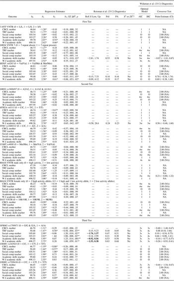
Regression estimates and differential susceptibility/diathesis–stress indices predicting overall effects (time intercepts) in the NICHD SECCYD

Note: Regression equation Y = b 0 + b 1X + b 2Z + b 3XZ, where X = parental sensitivity and Z = susceptibility genes (control variables not reported); RoS X, the regions of significance with respect to maternal sensitivity. Specifically, “low, up” represents the value of maternal sensitivity (standardized) below which and above which the regression of outcome on early sensitivity was statistically significant. PoI, the proportion of the interaction that fell above the cross-over point for the regressions; PA, the proportion of participants who had early sensitivity scores that fell above the crossover point; X 2 or ZX 2?”, whether X 2, ZX 2, or the set of both nonlinear terms together was statistically significant in the equation Y = b 0 + b 1X + b 2Z + b 3XZ + b 4X 2 + b 5ZX 2. For the Widaman et al. diagnostics, the AIC and BIC columns under the optimal model heading record the regression model that best fit the data based on the AIC and BIC information indices. In these columns, 1 = Model 1, 3w = Model 3w, 3s = Model 3s, 4 = Model 4w, 4s = Model 4s, and O indicates that although a non–main-effects' model fit the data best, the form of the interaction was contrary to prediction (e.g., the putatively more malleable group was estimated as being less malleable). Crossover represents the value of X (early sensitivity, standardized to M = 0, SD = 1) at which the regression lines intersected. If Model 3w or 3s fit the data best, both point and 95% CI interval estimates of the crossover point are given; if Model 4w or 4s fit best, the fixed crossover point of 2.00 is shown, and the 95% CI is inapplicable, because this crossover parameter was fixed. If Model 1 fit the data best, there was no crossover point, so both point and interval estimates are not applicable.
*p < .05.
aFalse discovery rate p < .05 (controlling Type I error across multiple tests [multiple dependent variables for each G × E interaction]; Benjamini & Hochberg, Reference Benjamini and Hochberg1995).
Roisman et al. approach
Each row in Table 3 represents a single intercepts as outcomes multilevel model, in which the interaction of early Maternal Sensitivity × Genetic Marker predicts the time intercept of each outcome variable.Footnote 1 For example, the first row of Table 3 displays the regression of mother-reported CBCL (i.e., the time intercept of CBCL across the 15-year period) onto the interaction of Early Maternal Sensitivity × 5-HTT VNTR. The multilevel models were specified with random time intercepts and random time slopes, although only random time intercepts were used as criterion variables, to be consistent with Roisman et al. (Reference Roisman, Newman, Fraley, Haltigan, Groh and Haydon2012). The time variable was centered at fifth grade, following Pluess and Belsky (Reference Pluess and Belsky2010) and Roisman et al. (Reference Roisman, Newman, Fraley, Haltigan, Groh and Haydon2012).
In Table 3, we see arrayed all six of the interaction effect diagnostics that were described in the introductory and listed in Table 1: RoS on X, PoI, PA, X 2 tests, a priori model comparisons, and crossover test. To explain these six diagnostics, we refer to the row in Table 3 in which DRD4 VNTR was the moderator and teacher-rated academic skills were the outcome. The first four columns in Table 3 give the traditional regression estimates from the model Y = b 0 + b 1X + b 2Z + b 3XZ, where X = early maternal sensitivity and Z = susceptibility gene DRD4 VNTR 7. These first four columns show that the interaction effect from the regression model is statistically significant (b 3 = 0.71, ΔR 2 = .010 for the interaction term XZ, and p = .03).Footnote 2
The second four columns give the interaction diagnostics recommended by Roisman et al. (Reference Roisman, Newman, Fraley, Haltigan, Groh and Haydon2012). For the RoS on X test, we see that the Y–Z relationship (i.e., the relationship between DRD4 VNTR 7 and academic skills) is statistically significant in the range above X = 1.74 (i.e., at high maternal sensitivity) and is also statistically significant in the opposite direction in the range below X = –2.81 (i.e., at low maternal sensitivity). Because the lower bound for the RoS on X (X = –2.81) falls outside the recommended range of ±2 SD from the mean of X, the RoS on X test fails to support either diathesis–stress or differential susceptibility. The next two Roisman et al. (Reference Roisman, Newman, Fraley, Haltigan, Groh and Haydon2012) diagnostics are the PoI and the PA the crossover. To support differential susceptibility, the PoI should be near 0.50 (ideally, PoI between 40% and 60%), and the PA index should be greater than 16% (see Roisman et al., Reference Roisman, Newman, Fraley, Haltigan, Groh and Haydon2012). For example, for the DRD4 VNTR 7 gene moderating the effect of maternal sensitivity on teacher-rated academic skills (11th row in Table 3), PoI = 0.53 and PA = 0.58. Thus, the PoI and the PA diagnostics both offer support for differential susceptibility in this case. Finally, for the nonlinearity diagnostic, we note that neither X 2, ZX 2, nor the combination of both X 2 and ZX 2 is statistically significant; thus this DRD4 VNTR 7 × Maternal Sensitivity interaction effect passes the nonlinearity test for inferring differential susceptibility. Overall, then, the form of the DRD4 VNTR 7 × Maternal Sensitivity interaction effect survives three of Roisman et al.'s (Reference Roisman, Newman, Fraley, Haltigan, Groh and Haydon2012) four diagnostics, but it fails the RoS on X test. Therefore, the Roisman et al. procedure yields the conclusion that differential susceptibility is not supported in the case of DRD4 VNTR 7.
Careful consideration of the many Roisman et al. (Reference Roisman, Newman, Fraley, Haltigan, Groh and Haydon2012) differential susceptibility tests reported in Table 3 reveals that few interaction effects meet the Roisman et al. criteria for differential susceptibility. First, we consider the three apparent interaction effects involving BDNF and HTR2A, as all three of these show the same pattern. That is, for the two interaction effects for the BDNF rs6265 gene (teacher-rated academic skills, and Woodcock–Johnson academic skills) and the one apparent interaction effect for the HTR2A rs6313 gene (Woodcock–Johnson academic skills), all three apparent interaction effects commonly fail the Benjamini–Hochberg (Reference Benjamini and Hochberg1995) procedure for Type I error control; fail the RoS on X test because the Y–Z relationship only becomes statistically significant at a value of X far above 2.0 SD above the mean of X (X = 7.33, 4.12, and 28.6, respectively); fail the PoI test that PoI should be near to 0.50 (PoI = 0.18, 0.19, and 0.24, respectively); pass the PA test, which requires that the percentage of the sample above the crossover point should be at or greater than 16% (% above = 16%, 17%, and 23%, respectively); and pass the nonlinearity test.
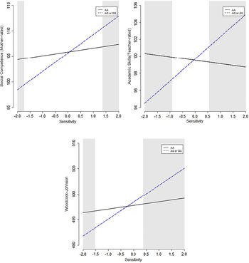
Second, and perhaps more promising, one genotype of a particular marker, OPRM1 rs1799971 AA +, seems to provide more support for a G × E interaction consistent with differential susceptibility. Specifically, five of six interaction effects involving OPRM1 rs1799971 AA+ and maternal sensitivity survive the Benjamini–Hochberg procedure, which controls for overall Type I Error (see Table 3). Of these five statistically–significant interaction effects: three pass the RoS on X test (mother-rated social competence, teacher-rated academic skills, and Woodcock–Johnson academic skills); four pass the PoI test and the PA test (only TRF teacher fails either of these two tests, because PoI = 0.10 and PA = 0.05); and all five pass the nonlinearity test. In brief, three interaction effects prove consistent with differential susceptibility (i.e., a true disordinal interaction), according to the Roisman et al. (Reference Roisman, Newman, Fraley, Haltigan, Groh and Haydon2012) diagnostics. These three differential susceptibility effects are the OPRM1 × Maternal Sensitivity interaction effects on mother-rated social competence, teacher-rated academic skills, and Woodcock–Johnson academic skills. These three differential susceptibility effects are plotted in Figure 1. Of note, in each of these three cases simple slopes analyses (i.e., RoS on Z tests) revealed that the association between the outcome and maternal sensitivity was positive and statistically significant in the hypothesized susceptible group (AA +, n = 455), but not in the comparison group (AG or GG, n = 128). Specifically, the association between social competence (mother rated) and maternal sensitivity was statistically significant in the AA group (b = 3.62, p < .001), but not in the AG|GG group (b = 0.75, p = .522). The association between academic skills and maternal sensitivity was statistically significant among those in the AA group (b = 3.33, p < .001), but not among those in the AG|GG group (b = 0.71, p = .391). The association between academic skills (teacher rated) and maternal sensitivity was statistically significant in the AA group (b = 2.61, p < .001), but not among those in the AG or GG group (b = –0.42, p = .631).
(Color online) Genetic Marker (OPRM1) × Environment (maternal sensitivity) interactions for mother-rated social competence, teacher-rated academic skills, and academic skills as assessed via the Woodcock–Johnson, respectively. The gray regions represent regions of significance.

The Widaman et al. approach
Next, we applied the Widaman et al. (Reference Widaman, Helm, Castro-Schilo, Pluess, Stallings and Belsky2012) criteria for G × E interaction data, the results of which are also displayed in Table 3. When inspecting these results, the following needs to be kept in mind regarding the signs of regression weights: the main (or lower order) effect of maternal sensitivity is shown in the b1 column in Table 3. The sign of the b 1 regression weight should be negative for the negative outcomes of problem behavior rated by mother (CBCL mother) and teacher (TRF teacher), but it should be positive for the remaining four outcome variables if higher levels of maternal sensitivity are associated with more competent functioning. Thus, higher levels of maternal sensitivity should be associated with lower levels of problem behavior, but higher levels of social competence and academic skills. Furthermore, each of the genetic moderators were coded exactly as in the Roisman et al. (Reference Roisman, Newman, Fraley, Haltigan, Groh and Haydon2012) approach, with higher numbers representing the hypothesized plasticity gene (see Table 2). Given this method of coding, the regression weight for the G × E interaction, shown in the b 3 column, should be negative for the two negative outcomes (problem behavior rated by mother and teacher) and positive for the remaining four outcome variables. That is, persons with more risk/plasticity alleles should exhibit a steeper negative slope as a function of maternal sensitivity for the negative outcome variables, but a stronger positive slope for the four positive outcomes. If results for a particular G × E interaction are the reverse of the predicted direction, this is regarded as a failure to confirm either the strong or weak diathesis–stress or differential-susceptibility hypotheses, given that these deal not only with the crossover point but also with the anticipated nature of the relation between predictor and outcome measure.
Table 4 presents an overall summary of the findings. Applying the Widaman et al. approach, 31 of the 78 investigated G × E interactions fitted the main-effects-only model (Model 1) best and in 23 cases support emerged for the differential-susceptibility or diathesis–stress model, with associations consistent with the hypothesized direction of gene action. In most of these instances, the data proved consistent with diathesis–stress, with 12 fitting the weak version (Model 4w) best and 5 fitting the strong version (Model 4s) best. In the remaining six instances in which the data fitted the differential-susceptibility model best, all but one fitted the strong version of the model best (Model 3s). In all other cases, a non–main-effects model fit the data best, but did not prove consistent with predictions and so is labeled “other” in Tables 3 and 4. Even though most of the differential-susceptibility or diathesis–stress related results generated using the Widaman et al. (Reference Widaman, Helm, Castro-Schilo, Pluess, Stallings and Belsky2012) method proved consistent with those obtained using the Roisman et al. (Reference Roisman, Newman, Fraley, Haltigan, Groh and Haydon2012) method, some differences emerged (see Table 3), and these are the exclusive focus of what follows.
Summary of findings

aThese are the results that survived Benjamini–Hochberg adjustment of alpha to avoid false discovery.
bThe non–main-effects' model fit the data best, but the form of the interaction was contrary to prediction.
In the case of DRD4, the weak diathesis–stress model (Model 4w) fitted the data best for teacher ratings of both problem behavior and social competence, and the strong diathesis–stress model (Model 4s) fitted best for Woodcock–Johnson academic skills. For academic skills as rated by teacher, the Akaike information criterion provided support for Model 3w, whereas the Bayesian information criterion supported Model 4w. Given the significance of the G × E interaction for this outcome, Model 3w estimates are displayed in Table 3. Both the point (–0.07) and interval estimates, 95% confidence interval (CI) = (–1.01, 0.87), fell well within the range of the distribution of the environment variable, leading to support for differential susceptibility. Recall that results using the Roisman et al. method indicated that children carrying the DRD4 7-repeat allele were more positively affected by maternal sensitivity than other children in the case of academic skills, whereas no differences between genotypes emerged when maternal sensitivity was low.
For DAT1, the Widaman et al. approach provided support for the weak diathesis–stress model (Model 4w) for two of the outcomes (teacher ratings of social competence and the Woodcock–Johnson measure of academic skills) contrary to the Roisman et al. approach, which yielded no significant G × E findings involving this polymorphism.
For the MAOA female data, DRD2, COMT, and TPH1, five interactions took the weak diathesis–stress form (Model 4w) and two the strong diathesis–stress form (Model 4s), none of which were detected using the Roisman et al. approach.
For the OPRM1 polymorphism, the Widaman et al. (Reference Widaman, Helm, Castro-Schilo, Pluess, Stallings and Belsky2012) criteria indicated that the strong differential susceptibility model (Model 3s) fitted the data best for all six outcomes. Moreover, the point and 95% CI interval estimates of the crossover points for all six dependent variables were consistent with differential susceptibility predictions. Specifically, the 6-point estimates each fell within 1 SD of the maternal sensitivity mean (range = –0.40 to 0.88), and the 95% CIs all fell within 2 SD of the mean on maternal sensitivity. According to the Roisman et al. (Reference Roisman, Newman, Fraley, Haltigan, Groh and Haydon2012) criteria, significant interactions emerged for five of the six dependent variables of which three met criteria for differential susceptibility.
Finally, in the case of CRHR1 rs7209436 and the prediction of mother-reported behavior problems, the strong differential susceptibility model (Model 3s) fitted the data best with the point estimate of the crossover point near the middle of maternal sensitivity, –0.44, and the 95% CI well within the range of the data, whereas in the case of the prediction of academic skills, the weak diathesis–stress model fitted the data best. Recall that the Roisman et al. method indicated no significant G × E findings involving CRHR1 rs7209436.
Reanalysis: Whites only
Due to concerns about risks associated with analyzing a multiethnic sample, all analyses were rerun focusing on the White subsample only; this resulted in only very modest changes in the results reported (and tabled). Although no new statistically significant results emerged using the Roisman et al. (Reference Roisman, Newman, Fraley, Haltigan, Groh and Haydon2012) approach, the few statistically significant results reported for OPRM1 in the full sample were no longer statistically significant when using the White-only sample (i.e., no results exceeded the false discovery rate in the White-only sample). More specifically, out of 78 G × E interaction effects estimated using the full sample, 69 had individual p values greater than .05, 9 had individual p values less than .05, and only 5 of these (i.e., OPRM1 effects) maintained p < .05 after controlling the false discovery rate. By comparison, in the White-only subsample, 68 of the 69 original analyses with individual p values greater than .05 remained as such (the one new effect with individual p < .05 was the DAT1 VNTR effect on WJ-R), 3 of the 9 analyses with individual p values less than .05 remained statistically significant in the White-only sample (i.e., BDNF and OPRM1 effects on teacher-rated academic skills, and HTR2A effect on WJ-R, maintained individual p < .05), but none of the effects in the White-only sample survived at p < .05 after controlling the false discovery rate. In short, the full-sample analyses only support a G × E interaction for 1 out of the 13 genetic variables assessed (i.e., OPRM1), and the White-only analyses support a G × E interaction for none of the 13 genetic variables assessed.
Discussion
Person × Environment interactions, whether involving genes, temperamental characteristics, or physiological factors, can take many forms. This report focused on two such forms and a variety of genetic polymorphisms: differential susceptibility, in which individuals carrying certain alleles prove more susceptible to both beneficial and adverse effects of supportive and risky environments, respectively; and diathesis–stress (or dual-risk), in which individuals carrying certain alleles prove more vulnerable to contextual adversity than do others. Here we sought to determine whether, and perhaps how, early maternal sensitivity/ insensitivity from 6 to 36 months of age interacted with each of a variety of candidate genes in predicting children's social, behavioral, and academic functioning through midadolescence.
This research is distinguished by its sample, the NICHD SECCYD. The relatively large NICHD SECCYD cohort, which was genotyped when participants were at age 15, has a number of strengths, including the genotyping of 12 putative plasticity genes (SNPs and VNTRs), structured in three tiers according to their evidentiary basis in the literature (see Table 2); the environmental factor of early maternal sensitivity, which is the most consistent predictor of children's functioning in the SECCYD (Belsky et al., Reference Belsky, Bakermans-Kranenburg and van IJzendoorn2007; Fraley et al., Reference Fraley, Roisman and Haltigan2013) and other investigations (e.g., Jaafari-Bimmel et al., Reference Jaffari-Bimmel, Juffer, van IJzendoorn, Bakermans-Kranenburg and Mooijaart2006; Sroufe et al., Reference Sroufe, Egeland, Carlson and Collins2005); six outcome assessments from multiple domains involving multiple informants; and outcomes assessed over multiple developmental assessments. Having noted these strengths, we would be remiss if we did not emphasize that, although larger than most of the studies on which the selection of the polymorphisms that were the focus of this report were based, the SECCYD is insufficiently large for estimating G × E effects that are modest in magnitude. For example, Duncan and Keller (Reference Duncan and Keller2011) contend that to estimate a large effect size for a single G × E interaction requires a sample of at least 600 subjects.
This research is also distinguished by its omnibus presentation of study results: specifically, 12 candidate gene polymorphisms interacting with early maternal sensitivity in the prediction of six repeatedly measured outcomes. We adopted this approach because questions have been raised about the confidence that can be placed in many reported findings across the sciences, including G × E interactions in the psychological sciences, the focus of this report. Along with many isolated effects of various SNPs and VNTRs on a host of psychological phenotypes, whether as main effects or in interaction with environmental factors, there have been numerous failures to replicate and evidence of false positives (Chabris et al., Reference Chabris, Hebert, Benjamin, Beauchamp, Cesarini and van der Loos2012; Charney & English, Reference Charney and English2012; Deary, Reference Deary2012). This has raised concerns that selective reporting of positive findings characterizes much of the published literature. The advantage of the omnibus approach is that it provides a bird's-eye view of a totality of possible G × E effects across a broad range of polymorphisms and outcomes using a strong, well-understood data set. The weakness, some might argue, is that such an omnibus approach may not be based on biologically plausible mechanisms by which particular genes come to influence particular phenotypes in interaction with particular environmental exposures. In addition, by focusing upon so many genes and so many dependent variables, adjustments for chance findings raises the bar for detecting significant effects, although interactions in uncorrected analyses were also generally nonsignificant.
A further distinguishing characteristic of this research is its analytic approach, which consists of two independently developed techniques designed to distinguish evidence for differential susceptibility from that of diathesis–stress (Roisman et al., Reference Roisman, Newman, Fraley, Haltigan, Groh and Haydon2012; Widaman et al., Reference Widaman, Helm, Castro-Schilo, Pluess, Stallings and Belsky2012). The need for new analytic techniques to evaluate evidence of differential susceptibility and diathesis–stress reflects the rapid influence these ideas have had on contemporary developmental science (e.g., Belsky & Pluess, Reference Belsky and Pluess2009; Ellis et al., Reference Ellis, Boyce, Belsky, Bakermans-Kranenburg and van IJzdenoorn2011). Originally, evidence for endogenous factors indicative of differential susceptibility was based on simple visual displays of data (Belsky, Reference Belsky, Ellis and Bjorklund2005); later, more formal criteria were established for assessing the presence of crossover interactions and the relative significance of simple slopes involved in interactions (Belsky et al., Reference Belsky, Bakermans-Kranenburg and van IJzendoorn2007; Kochanska et al., Reference Kochanska, Kim, Barry and Philibert2011).
The present analysis reflects further evolution in the assessment of differential susceptibility and diathesis–stress via the Roisman et al. (Reference Roisman, Newman, Fraley, Haltigan, Groh and Haydon2012) and Widaman et al. (Reference Widaman, Helm, Castro-Schilo, Pluess, Stallings and Belsky2012; Belsky et al., Reference Belsky, Pluess and Widaman2013) techniques. Recall that Roisman et al. (Reference Roisman, Newman, Fraley, Haltigan, Groh and Haydon2012) requires four criteria to be met for a determination of differential susceptibility: significant interaction terms using appropriate Type I error control; a RoI test demonstrating that outcomes and moderators (i.e., genetic polymorphisms) are related, with opposite signs (i.e., for better and for worse) at low and high values (i.e., within ±2 SD) of the environmental factor (i.e., maternal sensitivity); a substantial PoI (e.g., 40%–60%) and a substantial proportion of individuals (e.g., 16% or more) lying above the interaction crossover point; and the discounting of nonlinearities. Recall, too, that the Widaman et al. (Reference Widaman, Helm, Castro-Schilo, Pluess, Stallings and Belsky2012; Belsky et al., Reference Belsky, Pluess and Widaman2013) approach does not require a statistically significant interaction before further evaluating the nature of an interaction. Instead, it assesses the best fitting regression model that is reparameterized to highlight the interaction crossover point and its 95% confidence interval. Differential susceptibility is supported when the crossover occurs near the midpoint of the environmental predictor; diathesis–stress when the crossover point is at a high value of the predictor. The width of the confidence interval together with the placement of the crossover point affords insight into whether strong (typically small CI) or weak (typically large CI) forms of differential susceptibility or diathesis–stress are supported. The crossover point is freely modeled or set fixed to a high value of X, and fit indices indicate whether data accord best with models suggesting no interaction, or strong or weak forms of differential susceptibility or diathesis–stress.
When we applied these two methods to the SECCYD data, we found that most of the G × E interactions were weak or close to zero. Whereas maternal sensitivity proved again to be a consistent predictor of child functioning across the primary-school years, candidate polymorphisms did not show many main effects, nor did they tend to amplify or attenuate the predictive significance of maternal sensitivity/insensitivity. Only three interactions met the Roisman et al. (Reference Roisman, Newman, Fraley, Haltigan, Groh and Haydon2012) criteria for differential susceptibility, all involving the third-tier genetic marker OPRM1; and when analyses were restricted to only Whites, none of the previously detected effects survived at p < .05 after controlling the false discovery rate. In short, the full-sample analyses only support a G × E interaction for 1 out of the 13 genetic variables (12 markers but with the MAOA VNTR examined by sex) assessed (i.e., OPRM1), and the White-only analyses support a G × E interaction for none of the 13 genetic variables assessed.
Although there were more interactions supporting differential susceptibility using the Widaman et al. (Reference Widaman, Helm, Castro-Schilo, Pluess, Stallings and Belsky2012) technique, there were also more in which the diathesis–stress model proved the best fitting model. Many of the best fitting Widaman et al. (Reference Widaman, Helm, Castro-Schilo, Pluess, Stallings and Belsky2012) models supported weak versions of diathesis–stress or differential susceptibility. Moreover, one interaction, involving maternal sensitivity, DRD4 VNTR and teacher-rated academic skills, took the form of vantage sensitivity (Pluess & Belsky, Reference Pluess and Belsky2012), reflecting that one genetic subgroup proved disproportionately likely to benefit from supportive rearing while not being disproportionately susceptible to the adverse effects of maternal insensitivity. However, this same interaction did not survive controls for Type 1 error when using the Roisman et al. (Reference Roisman, Newman, Fraley, Haltigan, Groh and Haydon2012) approach. The consistent message across techniques and alternative samples, then, is that there are relatively few measured Gene × Early Maternal Sensitivity interactions in the NICHD SECCYD. Although acknowledgement of this result is important, it is equally important that the generally null G × E results reported here not be overgeneralized to other samples, other predictors, other outcomes, and other candidate genes.
What are other implications of these findings? One lesson may be to not privilege genetic variation over other endogenous characteristics when seeking to identify plasticity, or vulnerability, factors in development (Belsky & Pluess, Reference Belsky and Pluess2013; Kuo, Reference Kuo1967). When the focus has been on early negative emotionality/difficult temperament as the moderating plasticity or risk factor, consistent interactions reflecting both differential susceptibility and diathesis–stress have emerged using SECCYD data (Belsky & Pluess, 2010, Reference Belsky and Pluess2012; Roisman et al., Reference Roisman, Newman, Fraley, Haltigan, Groh and Haydon2012). Is is perhaps also notable that other SECCYD studies have detected evidence of G × E interaction (Belsky & Pluess, Reference Belsky and Pluess2013), although admittedly not using the new analytic approaches employed in the research reported herein. In sum, reflecting the larger scholarly literature, there are relatively few early Sensitivity × Gene interactions within the SECCYD. This does not preclude the possibility that plasticity and risk factors manifested in other forms may interact with maternal sensitivity to influence outcomes of developmental significance.
OPRM1 rs1799971 was an exception to the general lack of Gene × Early Maternal Sensitivity findings in this report. OPRM1, which is a polymorphism of the mu-opioid receptor gene, was listed as a third-tier SNP in Table 2 yet provided the strongest evidence for differential susceptibility. According to the Widaman et al. (Reference Widaman, Helm, Castro-Schilo, Pluess, Stallings and Belsky2012) analysis, the strong form of differential susceptibility was the best fitting model across four of six outcomes. According to the Roisman et al. (Reference Roisman, Newman, Fraley, Haltigan, Groh and Haydon2012) analysis, differential susceptibility was suggested on three of six outcomes: mother-rated social competence and academic skills (teacher-rated and Woodcock–Johnson performance), with diathesis–stress supported for teacher-rated problem symptomology and social competence. What the Roisman et al. (Reference Roisman, Newman, Fraley, Haltigan, Groh and Haydon2012) procedure found to be closer to diathesis–stress was inconsistently classified in Widaman et al. (Reference Widaman, Helm, Castro-Schilo, Pluess, Stallings and Belsky2012) as strongly fitting differential susceptibility using the Akaike information criterion index, but strongly fitting diathesis–stress using the Bayesian information criterion index.
The findings regarding OPRM1 are intriguing, but there are reasons to be cautious about interpreting even these limited G × E effects. The third-tier status of OPRM1 reflects the absence of a substantial knowledge base on this SNP (Troisi et al., Reference Troisi, Frazzetto, Carola, D'Amato, Moles and Siracusano2010, Reference Troisi, Frazzetto, Carola, Di Lorenzo, Coviello and Siracusano2012; Way et al., Reference Way, Taylor and Eisenberger2009). It is also of concern that the genetic subgroup that proves more susceptible to environmental variation is inconsistent across the few relevant G × E studies dealing with OPRM1-A/A carriers here and in one other report (Troisi et al., Reference Troisi, Frazzetto, Carola, Di Lorenzo, Coviello and Siracusano2012), but carriers of the G allele in another (Way et al., Reference Way, Taylor and Eisenberger2009). Moreover, the Roisman et al. (Reference Roisman, Newman, Fraley, Haltigan, Groh and Haydon2012) technique only controls for Type I error within but not across polymorphisms, which raises the possibility that our OPRM1 results reflect chance findings resulting from conducting analyses on 12 different polymorphisms. Of course, even the detected G × E interactions involving OPRM1 proved nonsignificant when the sample was restricted to Whites only and the false-discovery rate was controlled.
The aggregation of outcome variables over time in an intercepts as outcomes approach could be seen as a limitation of this study (Roisman et al., Reference Roisman, Newman, Fraley, Haltigan, Groh and Haydon2012) because reported analyses are not sensitive to developmental differences in the strength of G × E interactions. Notable in this regard is that Belsky and Pluess (Reference Belsky and Pluess2013) found that Gene × Childcare Quality interactions on caregiver-reported externalizing problems and teacher-reported social skills were evident at school entry but dissipated thereafter in a linear fashion. Might similar results have emerged had we set the intercept to earlier ages or assessed developmental trends as Belsky and Pluess (Reference Belsky and Pluess2013) did? As it turns out, preliminary analyses on the data included in the current report using the Roisman et al. (Reference Roisman, Newman, Fraley, Haltigan, Groh and Haydon2012) technique failed to provide support for this possibility (see footnote 1).
Perhaps the most significant limitation of this study is the candidate-gene approach itself. The use of candidate genes has the advantage, relative to behavioral-genetic designs, of actually measuring the biological substance of DNA. At their heart, though, both designs share the same problem: limited ability to speak to biological mechanisms (Plomin et al., Reference Plomin, Haworth, Meaburn, Price and Davis2013). A priori predictions linking genetic polymorphisms to domain-specific environmental features and outcomes are difficult without recourse to these explanatory mechanisms. For instance, what is it about DRD4, MAOA, OPRM1, or any other candidate gene that would interact with environmental variables in ways that are significant to long-term developmental adjustment? Charney and English (Reference Charney and English2012, p. 30) put the matter best: “The model of the relationship between genotype and phenotype used in the social sciences makes scientific discovery in genetics appear deceptively simple: All that is required is a large data set containing relevant behavioral data and genotype data consisting of several polymorphisms. … Statistical modeling takes care of the rest. However, the validity of these statistical models depends foundationally on the validity of the genetic paradigm they presuppose.” We agree with Rutter (Reference Rutter2009, p. 1288) that “biological plausibility” should be a central concern in the study of G × E processes. However, for now, the developmental biology linking genetic variation to complex psychological phenotypes is far more conjecture than it is science.
Alternatives to candidate-gene approaches have begun appearing in the literature, though the nature of the genetic paradigm they presuppose may still be evolving (Plomin, Reference Plomin2012). For example, polygenic approaches are being adopted in which candidate genes that do not yield a significant G × E interaction on their own have been found to amplify other candidate G × E interactions (Drury et al., Reference Drury, Gleason, Theall, Smyke, Nelson and Fox2012). Furthermore, genome-wide association analyses, which use hundreds of thousands of SNPs, permit estimation of general heritability among unrelated participants, as well as specific gene–outcome associations (Plomin et al., Reference Plomin, Haworth, Meaburn, Price and Davis2013).
Plomin (Reference Plomin2012, p. 11) writes that “once genes are found they will transform the ability of developmental research to address questions about developmental continuities, about psychopathological patterns, and about environmental risk patterns.” The rapid advance of technology that permits ever more comprehensive analyses of genetic phenomena, together with the irresistible allure of studying what most believe to be the irreducible element of life, our DNA, almost guarantees more and better research on the intersection of child development and molecular genetics. With this long-term vision, it is perhaps easier to accept that candidate-gene approaches, where effects are small and difficult to replicate and links to biological mechanism are tenuous, is just a first step down a grander path.
Clearly, results from the NICHD SECCYD do not suggest that candidate genetic markers are especially useful as endogenous precipitants of Person × Environment interactions, at least not involving maternal sensitivity and the 12 polymorphisms that are the focus of the current inquiry and the dependent variables considered. The effects that appeared were scattered, inconclusive, or as in the case of OPRM1, unusual, and failed to survive the false-discovery rate when only the White subsample was the focus of analysis. Other endogenous factors, and more advanced assessments of genetic phenomena, may be required to better appreciate the relative importance of differential susceptibility and diathesis–stress in modeling key adjustment markers of childhood and youth. Until then, the clearest message from this NICHD SECCYD report is that the benefits of sensitive mothering and the costs of insensitive mothering early in childhood are robust across a variety of potential genetic moderators.
Supplementary Materials
The supplementary materials mentioned in this article can be found online at http://journals.cambridge.org/dpp.