1. Introduction
Mortality events are incidents that lead to a marked increase in deaths within a population over a specific period. These events can have wide-ranging impacts on public health, the economy, and society at large. In contrast, longevity events refer to trends related to population aging and increased life expectancy. As people live longer, economic challenges arise, including prolonged retirement periods, strained pension systems, and increased public spending on healthcare. Given their profound economic consequences, it becomes a top priority for the insurance and financial services industry, academia, and government to find solutions for mitigating potential economic losses resulting from both mortality and longevity events.
The mortality rate underlying future deaths can be decomposed into an unsystematic component, which captures the idiosyncratic characteristics of individuals, and a systematic component, which is inherent to the entire population and governs mortality trends. While the unsystematic component can be diversified through pooling, the systematic component is undiversifiable. Life insurance is exposed to mortality risk, where actual mortality rates exceed expected, whereas pension funds face longevity risk, where participants live longer than projected. Consequently, both life insurers and pension providers are concerned with deviations of actual mortality rates from the norm.
The interaction of life insurers and pension providers with general investors in the capital market creates a channel to mitigate systematic mortality risk through financial securitization. Unlike traditional reinsurance, securitization as a capital market solution enables the transfer of mortality risk from life insurers or longevity risk from pension providers to the capital market. In particular, mortality-linked securities (MLSs) have emerged as a novel financial instrument for managing systematic mortality risk.Footnote 1
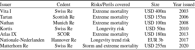
The first MLS, known as Vita I and sponsored by Swiss Re, was issued in December 2003, with a maturity of three years and an issue size of USD 400 million. Since then, a number of insurers and reinsurers have leveraged the capital market to securitize the mortality or longevity risks they face, with major deals prior to the COVID-19 pandemic collected in Table 1.Footnote 2
Examples of mortality-linked securities.

Meanwhile, the broader market for mortality and longevity risk transfers has experienced significant expansion. Blake et al. (Reference Blake, Cairns, Dowd and Kessler2019) provide a comprehensive review of successful capital market solutions for longevity and mortality risks, with a focus on longevity-linked instruments.
The outbreak of COVID-19, through its direct effects on mortality and indirect effects on capital markets, has posed new challenges for MLS development, as illustrated by the two examples below. Vita VI, the latest MLS sponsored by Swiss Re, issued in July 2021 with a maturity of five years and an issue size of USD 120 million, specifically excluded COVID-19-related deaths for the calendar year 2021 as per the deal terms. The La Vie Re 2021-1 mortality catastrophe bond, sponsored by Minnesota Life Insurance Company with an issue size of USD 100 million, was scheduled to launch in December 2021 but was withdrawn due to limited investor support prompted by concerns over the pandemic. These examples highlight an imperative need for developing a framework that accurately models and prices mortality risk.
To undertake this task, it is essential to develop a pricing framework that accounts for the intricate and multifaceted relationship between mortality rates and financial market performance. Mortality rates are influenced by the overall economic conditions within a country or region. A robust economy tends to elevate living standards, improve healthcare, and consequently reduce mortality rates, while a weak economy has the opposite effect. Moreover, substantial market declines can trigger stress and anxiety, potentially impacting both individual and collective health. Conversely, mortality events, such as pandemics and health crises, can directly or indirectly affect financial market performance, including disrupted business activities, decreased consumer spending, and shifts in risk perception and sentiment. Some of these factors may trigger a cascade of consequences across various asset classes and industries.
The relationship between mortality rates and financial market performance has remained a focal point in demographic economics for several decades. Early discussions on this topic can be traced back to Preston (Reference Preston1975). An extensive body of research, including Hanewald (Reference Hanewald2011), Niu and Melenberg (Reference Niu and Melenberg2014), Carvalho et al. (Reference Carvalho, Ferrero and Nechio2016), and Schwandt (Reference Schwandt2018), provides a wealth of empirical evidence and insights. Recently, the COVID-19 pandemic has inspired a new wave of research into this relationship; see, for example, Zhang et al. (Reference Zhang, Hu and Ji2020) and Li et al. (Reference Li, Liu, Tang and Yuan2023), among many others. Note that correlation in this literature does not necessarily imply causation.
In this paper, we employ a general jump-diffusion modeling framework to describe the dynamics of financial and mortality risks. Our model captures the correlation between them and accounts for potential jumps. This aligns closely with recent studies by Li et al. (Reference Li, Liu, Tang and Yuan2023), Arık et al. (Reference Arık, Ugŭr and Kleinow2023), and Deelstra et al. (Reference Deelstra, Devolder and du Vivier2024), who challenge the traditional assumption of independence between financial and mortality risks, propose and empirically test a similar dynamic relationship, and explore its implications for pricing various novel life insurance products.
The pricing of life insurance products is central to life insurance and pension research, particularly in the current era, as hybrid products that blend insurance and financial features continue to emerge. The well-established arbitrage pricing theory naturally emerges as a primary method; see, for example, Milevsky and Promislow (Reference Milevsky and Promislow2001), Blanchet-Scalliet et al. (Reference Blanchet-Scalliet, El Karoui and Martellini2005), Cairns et al. (Reference Cairns, Blake and Dowd2006), and Bayraktar et al. (Reference Bayraktar, Milevsky, Promislow and Young2009).Footnote 3 However, the MLS market is far from complete, making it difficult to decide which pricing measure to use. To address this incompleteness issue, various alternative pricing approaches have been developed in the literature, such as probability transform (Lin and Cox, Reference Lin and Cox2005; Wills and Sherris, Reference Wills and Sherris2010), risk minimization (Dahl and Møller, Reference Dahl2006; Biagini et al., Reference Biagini, Botero and Schreiber2017), entropy minimization (Li and Ng, Reference Li and Ng2011; Tang and Li, Reference Tang and Li2021), tâtonnement or supply-demand methods (Chen et al., Reference Chen, Sherris, Sun and Zhu2013; Zhou et al., Reference Zhou, Li and Tan2015), market-consistent valuation (Malamud et al., Reference Malamud, Trubowitz and Wüthrich2008; Pelsser and Stadje, Reference Pelsser and Stadje2014; Dhaene et al., Reference Dhaene, Stassen, Barigou, Linders and Chen2017; Deelstra et al., Reference Deelstra, Devolder, Gnameho and Hieber2020), and utility indifference pricing (Dahl and Møller, Reference Dahl2006; Ludkovski and Young, Reference Ludkovski and Young2008; Chen et al., Reference Chen, Sherris, Sun and Zhu2013). Given their distinct considerations and justifications, no single approach can be deemed universally superior, as noted by Bauer et al. (Reference Bauer, Börger and Ruß2010).
Among these approaches, we highlight the indifference pricing approach. Consider an agent evaluating the sale of a security with a contingent claim at a future time
 $T\gt0$
. The utility indifference price is defined as the value
 $p$
at which the agent is indifferent to engaging in the transaction, in the sense that their expected utility under optimal trading remains the same whether they receive the price
 $p$
now and settle the payoff at
 $T$
, or forgo both the payment now and the settlement at
 $T$
. Note that
 $p$
represents the seller’s indifference price. In this work, we adopt the indifference pricing approach for its sound economic justifications and its ability to leverage advanced backward stochastic differential equation (BSDE) techniques.
Since its introduction by Hodges and Neuberger (Reference Hodges and Neuberger1989), the indifference pricing approach has been widely applied in incomplete markets. Early contributions include Davis et al. (Reference Davis, Panas and Zariphopoulou1993), Rouge and El Karoui (Reference Rouge and El Karoui2000), and Hu et al. (Reference Hu, Imkeller and Müller2005). Moreover, Carmona (Reference Carmona2009) collects a series of papers providing a comprehensive account of the topic. Among these, Henderson and Hobson (Reference Henderson, Hobson and Carmona2009) offer an excellent overview of the indifference pricing approach and present several compelling arguments in its favor. The indifference pricing approach works solely under the physical measure, thereby circumventing the issue of identifying a pricing measure. Building on the notion of certainty equivalent, this approach allows for the incorporation of risk aversion. Moreover, the resulting indifference price is generally nonlinear in the quantity of a claim. These arguments are particularly relevant for the pricing of various insurance products. Accordingly, it is not surprising that there is an active strand of the insurance literature that employs the indifference pricing approach. See, for example, Young and Zariphopoulou (Reference Young and Zariphopoulou2002), Becherer (Reference Becherer2003), Ludkovski and Young (Reference Ludkovski and Young2008), Delong (Reference Delong2013), Chen and Delong (Reference Chen2015), and Liu et al. (Reference Liu, Tang and Yuan2021), just to name a few that share similarities with our present study.
Utility indifference pricing typically involves solving two related optimization problems linked to the agent’s decision on whether or not to engage in the security under consideration. Within the Markovian setting, these problems are often solved using the dynamic programming principle, resulting in a Hamilton–Jacobi–Bellman (HJB) partial differential equation for the associated value function. However, this technique may not be applicable in more general settings in which the coefficients of Itô processes are stochastic or depend on both present and past values of the underlying processes, or in which the payoffs are path-dependent. These features characterize our setting; see Section 2 for details. In such cases, the dynamic programming principle typically leads to a BSDE. See Lim (Reference Lim2004), Becherer (Reference Becherer2006), and Delong (Reference Delong2013) for related discussions. Therefore, we opt to apply BSDE techniques in this work.
The BSDE literature is extensive and continues to evolve. Early work focuses on the Brownian setting, tracing back to Bismut (Reference Bismut1973) for the linear case and to Pardoux and Peng (Reference Pardoux and Peng1990) for the general nonlinear case. Since then, BSDEs have become a central tool in stochastic control. Subsequent contributions extend the theory to settings with jumps and have led to a broad range of applications, notably in mathematical finance. In particular, BSDEs have been widely used in utility maximization and utility indifference pricing in incomplete markets.
While we refrain from providing a comprehensive review of this vast literature, we cite several representative studies that guide our work. Tang and Li (Reference Tang and Li1994) are among the earliest to introduce random jumps characterized by a Poisson point process and to establish a maximum principle. Hu et al. (Reference Hu, Imkeller and Müller2005) study the utility maximization problem in a Brownian setting and apply the martingale optimality principle to derive a BSDE characterization of the value process. Becherer (Reference Becherer2006) analyzes BSDEs driven by a Brownian motion and a random measure and solves various stochastic optimization problems with exponential utility in a setting with diffusion-type stock prices and a discontinuous underlying filtration. Morlais (Reference Morlais2009) considers utility maximization in a univariate setting driven by a Wiener process and a Poisson point process with a finite Lévy measure and establishes existence and uniqueness for quadratic BSDEs, while Morlais (Reference Morlais2010) extends the analysis to the case allowing an infinite Lévy measure. Laeven and Stadje (Reference Laeven and Stadje2014) consider a setting with both a diffusion and a general jump component, incorporate ambiguity-averse preferences into the model, and establish existence and uniqueness for a general class of BSDEs. Mereu and Stelzer (Reference Mereu and Stelzer2017) investigate exponential utility maximization in a market driven by a Lévy pure-jump process, focusing on structural properties of the associated BSDEs. Most of the studies reviewed above assume a bounded terminal claim, with the exception of Tang and Li (Reference Tang and Li1994) and Mereu and Stelzer (Reference Mereu and Stelzer2017), who focus on theoretical developments rather than explicit solutions. Taken together, these studies highlight the versatility of BSDE techniques for utility maximization problems, with key advantages including numerical tractability via Monte Carlo simulation and the flexibility to accommodate nonconvex constraints. This motivates our adoption of BSDE techniques. Finally, we refer to Delong (Reference Delong2013) for a textbook treatment of BSDEs with a focus on jumps and actuarial applications.
Therefore, our work builds on three strands of literature: mortality-linked securities, utility indifference pricing, and BSDEs. We propose an integrated modeling framework in which financial and mortality risks jointly follow a multivariate Itô process driven by both a multivariate Brownian motion and a Poisson point process. This model captures gradual variations, sudden shocks, and the dynamic relationship between these two risk sources, making it particularly appealing for pricing MLSs as well as for empirical and numerical studies.
Our goal is to price a general MLS with a bounded payoff. We adopt the utility indifference approach, which operates under the physical measure, incorporates risk aversion, and captures how prices respond to the joint dynamics of financial and mortality risks. To determine the utility indifference price, we leverage BSDE techniques, which are well suited to non-Markovian settings. Building on the results of Tang and Li (Reference Tang and Li1994) for BSDEs with Lipschitz generators and on the martingale optimality principle of Hu et al. (Reference Hu, Imkeller and Müller2005), we fully characterize the value process and the optimal investment strategy in this multivariate, jump-inclusive setting. Relative to Morlais (Reference Morlais2009, Reference Morlais2010) and Mereu and Stelzer (Reference Mereu and Stelzer2017), we consider a multivariate setting driven by both diffusion and jump components, and, in particular, our setting allows for the interplay between financial and mortality risks, a key feature of our consideration. More broadly, our methodology, combining utility indifference pricing with BSDE techniques, applies to other pricing tasks in incomplete markets.
Finally, we conduct numerical studies on the valuation of several MLSs, including S-forward contracts, longevity caplets, and unit-linked securities, with a focus on sensitivity analysis of the resulting indifference prices against various key model parameters. To facilitate our numerical implementation, we assume that the risky asset price follows a stochastic volatility model similar to that of Jones (Reference Jones2003) and that the mortality rate follows an affine jump-diffusion process as in Bravo and Nunes (Reference Bravo and Nunes2021), with dependence through their diffusion components. Our results demonstrate that the parameters of the mortality rate process have a more pronounced effect on pricing than those governing the asset price dynamics and that the correlation between the risky asset price and the mortality rate plays a significant role in pricing.
The rest of the paper is organized as follows: Section 2 sets up the modeling framework, including the underlying dynamics and utility indifference pricing; Section 3 develops BSDE techniques for utility indifference pricing; Section 4 presents numerical studies to illustrate our main results; Section 5 concludes the work with a few remarks; and finally, Appendix A collects several technical steps used to establish our main result, along with some additional details.
2. The utility indifference pricing framework
All economic activities are assumed to take place on a time horizon
 $\left[0,T\right] $
for some
 $T\gt0$
. We work in a probability space
 $(\Omega ,\mathcal{F},P)$
, which is rich enough to accommodate an
 $m$
dimensional standard Brownian motion
 $\boldsymbol{W}=\left\{ \boldsymbol{W}(t)\right\}_{0\leq t\leq T}=\left\{ (W_{1}(t),\ldots ,W_{m}(t))^{\intercal }\right\}_{0\leq t\leq T}$
and a Poisson random measure
 $N$
on
 $[0,T]\times \mathbb{R}^{n}$
with compensator
 $\nu (dt,d\boldsymbol{x})=\eta (d\boldsymbol{x})dt$
, where
 $\eta (\!\cdot\!)$
is a finite measure on
 $\mathbb{R}^{n}$
. The corresponding compensated Poisson random measure is denoted by
 $\tilde{N}(dt,d\boldsymbol{x})$
. Let
 $\mathbb{F}=\left\{ \mathcal{F}_{t}\right\}_{0\leq t\leq T}$
be the natural filtration associated with
 $\boldsymbol{W}$
and
 $N$
, assumed to satisfy the usual conditions of
 $P$
completeness and right-continuity. Without loss of generality, we assume that
 $\boldsymbol{W}$
and
 $N$
are independent; see, for example, Theorem 6.3 in Chapter II of Ikeda and Watanabe (Reference Ikeda and Watanabe1981). As usual,
 $1_{(\cdot)}$
denotes the indicator function of an event
 $(\!\cdot\!)$
.
In the following subsections, we present models for asset prices in the financial market and a reference mortality rate and then discuss the general utility indifference pricing framework.
2.1. The financial market
We consider a financial market with one risk-free asset, assumed to have a zero interest rate, and
 $d$
risky assets, whose prices per share at time
 $t$
are denoted by
 $S_{1}(t)$
, …,
 $S_{d}(t)$
. The zero interest rate assumption is made without loss of generality, as explained in Remark 2.1 below. The vector process
 $\left\{ \boldsymbol{S}(t)\right\}_{0\leq t\leq T}=\left\{ \left( S_{1}(t),\ldots ,S_{d}(t)\right) ^{\intercal}\right\} _{0\leq t\leq T}$
, with
 $\boldsymbol{S}(0)\gt\boldsymbol{0}$
understood componentwise, satisfies the system of stochastic differential equations (SDEs)
 \begin{equation}\frac{dS_{i}(t)}{S_{i}(t{\kern.5pt}{-}{\kern-.8pt})}=\mu _{i}(t)dt+\sum_{j=1}^{m}\sigma_{i,j}(t)dW_{j}(t)+\int_{\mathbb{R}^{n}}\theta _{i}(t,\boldsymbol{x})\tilde{N}(dt,d\boldsymbol{x}),\qquad t\in \left[ 0,T\right] ,i=1,\ldots ,d. \end{equation}
The vectors
 $\boldsymbol{\mu }(t)=\left( \mu _{1}(t),\ldots ,\mu_{d}(t)\right) ^{\intercal }\in \mathbb{R}^{d}$
and
 $\boldsymbol{\theta }(t,\boldsymbol{x})=\left( \theta _{1}(t,\boldsymbol{x}),\ldots ,\theta _{d}(t,\boldsymbol{x})\right) ^{\intercal }\gt-\boldsymbol{1}$
and the matrix
 $\Sigma (t)=\left( \sigma _{i,j}(t)\right) \in \mathbb{R}^{d\times m}$
are all assumed to be uniformly bounded and
 $\mathbb{F}$
predictable, so that (2.1) admits a unique strong solution, which is further assumed to be positive; see, for example, Theorem 37 in Chapter II of Protter (Reference Protter2005). We assume that, a.e. with respect to
 $dP\mathcal{\otimes }dt$
,
 $\Sigma (t)$
has full rank, and there exist constants
 $\zeta \gt\varepsilon \gt0$
such that
 $\zeta I_{d}-\Sigma (t)\Sigma ^{\intercal }(t)$
and
 $\ \Sigma (t)\Sigma^{\intercal }(t)-\varepsilon I_{d}\ $
are positive semidefinite, where
 $I_{d} $
represents the identity matrix of dimension
 $d$
. Other than these assumptions, the model is general and covers most popular jump-diffusion models.
2.2. The mortality rate process
We consider a general MLS. By the very definition, an appropriate mortality model is central to establishing the pricing framework. The literature on this topic is extensive, largely inspired by reduced-form models in credit risk theory. We refer the reader to Dahl (Reference Dahl2004), Biffis (Reference Biffis2005), Bauer and Kramer (Reference Bauer and Kramer2016), and Bravo and Nunes (Reference Bravo and Nunes2021), to mention just several. These works model mortality rates as affine processes for analytical and computational tractability.
Following this strand of literature, we consider a general model for the mortality rate process
 $\{\lambda (t)\}_{0\leq t\leq T}$
, evolving according to
 \begin{equation}d\lambda (t)=\mu _{\lambda }(t)dt+\sum_{j=1}^{m}\sigma _{\lambda,j}(t)dW_{j}(t)+\int_{\mathbb{R}^{n}}\theta _{\lambda }(t,\boldsymbol{x})\tilde{N}(dt,d\boldsymbol{x}),\qquad t\in \left[ 0,T\right] ,\end{equation}
where
 $\mu _{\lambda }(t)\in \mathbb{R}$
,
 $\theta _{\lambda }(t,\boldsymbol{x})\in \mathbb{R}$
, and
 $\boldsymbol{\sigma }_{\lambda }(t)=\left( \sigma_{\lambda ,1}(t),\ldots ,\sigma _{\lambda ,m}(t)\right) ^{\intercal }\in\mathbb{R}^{m}$
are assumed to be
 $\mathbb{F}$
predictable processes and such that the integrals involved exist and (2.2) admits a unique strong solution; see, for example, Theorem 1.19 of Øksendal and Sulem (Reference Øksendal and Sulem2019). This covers, in particular, the class of affine mortality models. Note that
 $\{\lambda (t)\}_{0\leq t\leq T}$
in equation (2.2) should be interpreted as the mortality rate of a representative population rather than that of an individual. The model can also be applied to extreme mortality risk, as in Li et al. (Reference Li, Liu, Tang and Yuan2023), with
 $\{\lambda (t)\}_{0\leq t\leq T}$
interpreted accordingly as excess mortality.
It is straightforward to further specify the coefficients to ensure the positivity of the solution
 $\{\lambda (t)\}_{0\leq t\leq T}$
. However, we choose not to impose this restriction but instead allow
 $\{\lambda(t)\}_{0\leq t\leq T}$
to take negative values, in which case the coefficients can be adjusted to render the corresponding probability arbitrarily small. As recently discussed by Liu et al. (Reference Liu, Liu, Tang and Zhu2026), allowing for negative mortality rates, much like negative interest rates, has practical relevance. For example, in estimation, it can help address accounting issues in which over-counting at a previous time point needs to be corrected by subtracting the excess. Often, these accounting adjustments lead to sudden upward or downward changes in estimated mortality rates, which in turn justify both positive and negative jumps in the mortality rate process. This feature can be captured, for example, by using an asymmetric double exponential distribution, as assumed by Bravo and Nunes (Reference Bravo and Nunes2021) in their proposed affine jump–diffusion model for the mortality rate process.
2.3. Utility indifference pricing
Since the market for MLSs is typically incomplete, we employ the utility indifference pricing approach for addressing this incompleteness. Consider an agent—always specified as the issuer or provider of the MLS in this work—who faces a liability represented by a bounded
 $\mathcal{F}_{T}$
measurable random variable
 $C$
, payable at the terminal time
 $T$
. This means that the liability is a general payout contingent on the performance of both the financial market and the mortality rate. Our objective is to determine the utility indifference price
 $p$
at time 0 of the payoff
 $C$
. This price
 $p$
is defined as the value at which the agent is indifferent, meaning that the expected utility under optimal trading is unchanged between (i) receiving
 $p$
at time 0 and settling the payoff
 $C$
at time
 $T$
and (ii) not receiving
 $p$
at time 0 and therefore not settling the payoff
 $C$
at time
 $T$
.
Suppose the agent, with initial wealth of
 $w$
at time 0, invests at each time
 $t\in \left[ 0,T\right] $
an amount
 $\pi _{i}(t)$
in the
 $i$
th risky asset,
 $i\in \left\{ 1,\ldots ,d\right\} $
. In particular, we assume that the process
 $\left\{ \boldsymbol{\pi }(t)\right\} _{0\leq t\leq T}=\{\left(\pi _{1}(t),\ldots ,\pi _{d}(t)\right) ^{\intercal }\}_{0\leq t\leq T}$
belongs to an admissible set
 $\mathcal{A}$
, which consists of all
 $\mathbb{F}$
predictable processes with values in a bounded and closed subset of
 $\mathbb{R}^{d}$
. The wealth
 $X^{w,\boldsymbol{\pi }}(t)$
, accumulated from time 0 to
 $t$
, is then given by
 \begin{equation}X^{w,\boldsymbol{\pi }}(t)=w+\int_{0}^{t}\boldsymbol{\pi ^{\intercal }}(s)\left( \boldsymbol{\mu }(s)ds+\Sigma (s)d\boldsymbol{W}(s)+\int_{\mathbb{R}^{n}}\boldsymbol{\theta }(s,\boldsymbol{x})\tilde{N}(ds,d\boldsymbol{x})\right) , \end{equation}
which is well defined due to the boundedness of the strategies and the coefficients in (2.1).
Assume that the agent has an exponential utility, with a risk aversion parameter
 $\alpha \gt0$
:
 \begin{equation}U(y)=-e^{-\alpha y},\qquad y\in \mathbb{R}. \end{equation}
Exponential utility is widely employed in finance, insurance, and economics, largely due to its analytical tractability. Although it may be unrealistic in certain scenarios, it offers several practical advantages. In particular, it accommodates real-valued wealth, which is essential when modeling both the purchase and sale of securities, and it yields optimal decisions that are independent of initial wealth, thereby supporting pricing consistency across market participants with heterogeneous endowments.Footnote 4
Define the value function
 \begin{equation}V(w,q)=\sup_{\boldsymbol{\pi }\in \mathcal{A}}E\left[ U\left( X^{w,\boldsymbol{\pi }}(T)-qC\right) \right] ,\qquad q\geq 0. \end{equation}
Thus, the utility indifference price
 $p$
is the solution to
 \begin{equation}V(w,0)=V(w+p,1). \end{equation}
Given the agent’s exponential utility function, we notice that
 $V(w,q)=e^{-\alpha w}V(0,q)$
. Hence, relation (2.6) reduces to
 $e^{-\alpha w}V(0,0)=e^{-\alpha (w+p)}V(0,1)$
, which yields a representation of the indifference price as
 \begin{equation}p=\frac{1}{\alpha }\ln \frac{V(0,1)}{V(0,0)}. \end{equation}
Along the same lines, we can derive the indifference price
 $p$
(
 $q$
) for the payoff
 $qC$
with
 $q\gt0$
, and it is easy to further show that
 $p$
(
 $q$
) is convex in the quantity
 $q$
. See Section 2.3 of Carmona (Reference Carmona2009) for related discussions.
Remark 2.1. The zero interest rate assumption for the risk-free asset entails no loss of generality and is commonly adopted in the literature; see, for example, Subsection 1.2.5 of Karatzas and Kardaras (Reference Karatzas and Kardaras2021). Our model remains fully general even when a nontrivial risk-free rate is present, provided that the stock prices, payoffs, investment strategies, and wealth are interpreted as being discounted by the risk-free rate, and the stock returns are understood as expressed in excess of the risk-free rate. Under this interpretation, the zero interest rate assumption reflects a choice of numéraire and imposes no restriction on the dynamics of the financial market.
3. The BSDE method for utility indifference pricing
In this section, we solve the optimization problem (2.5) using a BSDE technique. We assume
 $w=0$
without loss of generality and denote the wealth process (2.3) by
 $\left\{ X^{\boldsymbol{\pi }}(t)\right\}_{0\leq t\leq T}$
.
Before discussing the BSDE technique, we need to set up some notational conventions:
-
• For
 $1\leq r\leq \infty $
,
$\mathcal{S}^{r}$
denotes the set of
$\mathbb{F}$
adapted processes
$Y$
, right-continuous with left limits and taking values in
$\mathbb{R}$
, satisfying
\begin{equation*}\left( E\left[ \sup_{t\in \left[ 0,T\right] }\left\vert Y(t) \right\vert ^{r}\right] \right) ^{\frac{1}{r}}\lt\infty .\end{equation*}
-
•
$\mathcal{L}^{2,m}$
denotes the set of
$\mathbb{F}$
predictable processes
$\boldsymbol{Z}$
taking values in
$\mathbb{R}^{m}$
, satisfyingwhere
\begin{equation*}\left( E\left[ \int_{0}^{T}\left\Vert \boldsymbol{Z}(s)\right\Vert ^{2}ds\right] \right) ^{\frac{1}{2}}\lt\infty ,\end{equation*}
$\left\Vert \cdot \right\Vert $
denotes the Euclidean norm on the space
$\mathbb{R}^{m}$
.
-
•
$H_{\eta }^{2}$
denotes the set of measurable functions
$k\,:\,\mathbb{R}^{n}\rightarrow \mathbb{R}$
, satisfyingwhere
\begin{equation*}\left\Vert k\right\Vert _{2,\eta }=\left( \int_{\mathbb{R}^{n}}k^{2}(\boldsymbol{x})\eta (d\boldsymbol{x})\right) ^{\frac{1}{2}}\lt\infty ,\end{equation*}
$\eta $
is the finite measure in defining the Poisson random measure
$N $
.
-
•
$\mathcal{L}_{\eta }^{2}$
denotes the set of
$\mathbb{F}$
predictable processes
$K\,:\,\Omega \times \lbrack 0,T]\times \mathbb{R}^{n}\rightarrow\mathbb{R}$
, satisfying Observe that the condition
\begin{equation*}\left( E\left[ \int_{0}^{T}\int_{\mathbb{R}^{n}}K^{2}(s,\boldsymbol{x})\eta(d\boldsymbol{x})ds\right] \right) ^{\frac{1}{2}}\lt\infty .\end{equation*}
$K\in \mathcal{L}_{\eta }^{2}$
implies that
$K(t,\cdot )\in H_{\eta }^{2}$
a.e. with respect to
$dP\mathcal{\otimes }dt$
.
-
• A generator is a function
$f\,:\,\Omega \times \left[ 0,T\right] \times\mathbb{R\times R}^{m}\times H_{\eta }^{2}$
$\rightarrow \mathbb{R}$
that is
$\mathcal{P\otimes B}(\mathbb{R}^{m+1})\mathcal{\otimes B}(H_{\eta }^{2})$
measurable, where
$\mathcal{P}$
denotes the predictable
$\sigma $
-algebra on
$\Omega \times \left[ 0,T\right] $
. Moreover, a generator
$f$
is called Lipschitz if there exists a constant
$c\geq 0$
such that the inequality holds a.e. with respect to
\begin{equation*}\left\vert \, f(\omega ,t,y_{1},\boldsymbol{z}_{1},k_{1})-f(\omega ,t,y_{2},\boldsymbol{z}_{2},k_{2})\right\vert \leq c\left( \left\vert y_{1}-y_{2}\right\vert +\left\Vert \boldsymbol{z}_{1}-\boldsymbol{z}_{2}\right\Vert +\left\Vert k_{1}-k_{2}\right\Vert _{2,\eta }\right)\end{equation*}
$dP\mathcal{\otimes }dt$
for any triplets
$(y_{1},\boldsymbol{z}_{1},k_{1})$
and
$(y_{2},\boldsymbol{z}_{2},k_{2})$
from
$\mathbb{R\times R}^{m}\times H_{\eta }^{2}$
. We will write
$f(t,y,\boldsymbol{z},k)$
for simplicity as long as no confusion arises.


To find the value function and an optimal strategy for (2.5), we follow Hu et al. (Reference Hu, Imkeller and Müller2005) to seek a family of stochastic processes
 $\left\{R^{\boldsymbol{\pi }}\right\} _{\boldsymbol{\pi }\in \mathcal{A}}$
fulfilling the following properties:
-
•
$R^{\boldsymbol{\pi }}(T)=-e^{-\alpha (X^{\boldsymbol{\pi }}(T)-C)}$
for all
$\boldsymbol{\pi }\in \mathcal{A}$
; -
•
$R^{\boldsymbol{\pi }}(0) =R(0) $
is constant for all
$\boldsymbol{\pi}\in \mathcal{A}$
; -
•
$\{R^{\boldsymbol{\pi }}(t)\}_{0\leq t\leq T}$
is a supermartingale for all
$\boldsymbol{\pi }\in \mathcal{A}$
, and there exists a strategy
$\boldsymbol{\pi }_{\ast }\in \mathcal{A}$
such that
$\{R^{\boldsymbol{\pi }_{\ast }}(t)\}_{0\leq t\leq T}$
is a martingale.


If
 $R^{\boldsymbol{\pi }}$
is from such a family, then
 \begin{equation}E\left[ R^{\boldsymbol{\pi }}(T)\right] =E\left[ -e^{-\alpha (X^{\boldsymbol{\pi }}(T)-C)}\right] \leq R(0)=E\left[ -e^{-\alpha (X^{\boldsymbol{\pi }_{\ast }}(T)-C)}\right] =V(0,1), \end{equation}
which implies that
 $\boldsymbol{\pi }_{\ast }$
is an optimal strategy. To construct such a family, set
 \begin{equation}R^{\boldsymbol{\pi }}(t)=-e^{-\alpha (X^{\boldsymbol{\pi }}(t)-Y(t))},\qquad t\in \lbrack 0,T],\boldsymbol{\pi }\in \mathcal{A}, \end{equation}
such that
 $(Y,\boldsymbol{Z},K)\in \mathcal{S}^{\infty }\times\mathcal{L}^{2,m}\times \mathcal{L}_{\eta }^{2}$
is a solution to the BSDE
 \begin{eqnarray}Y(t) &=&C+\int_{t}^{T}f\left( s,Y(s-),\boldsymbol{Z}(s),K(s,\cdot )\right) ds\notag \\&&-\int_{t}^{T}\boldsymbol{Z}^{\intercal }(s)d\boldsymbol{W}(s)-\int_{t}^{T}\int_{\mathbb{R}^{n}}K(s,\boldsymbol{x})\tilde{N}(ds,d\boldsymbol{x}), \end{eqnarray}
where
 $f$
is a generator.
To solve (2.5), we aim to find a generator
 $f=f_{\ast }$
for which equation (3.3) admits a unique solution and
 $\{R^{\boldsymbol{\pi }}(t)\}_{0\leq t\leq T}$
is a supermartingale for all
 $\boldsymbol{\pi }\in \mathcal{A}$
, as well as a strategy
 $\boldsymbol{\pi }_{\ast }\in\mathcal{A}$
such that
 $\{R^{\boldsymbol{\pi }_{\ast }}(t)\}_{0\leq t\leq T}$
is a martingale. We achieve these goals in the following theorem, which is the main result of this paper. Notably, the generator satisfying these conditions does not depend on the process
 $\{Y(t)\}_{0\leq t\leq T}$
due to the exponential utility.
Theorem 3.1. For every
 $\mathcal{F}_{T}$
measurable and bounded random variable C:
-
(i) There exists a unique solution
$(Y,\boldsymbol{Z},K)\in \mathcal{S}^{\infty }\times \mathcal{L}^{2,m}\times \mathcal{L}_{\eta}^{2}$
to the BSDE (3.4)where, for every
\begin{eqnarray}Y(t) &=&C+\int_{t}^{T}\mathop{\mathrm{ess\,inf}}\limits_{\boldsymbol{\pi }\in \mathcal{A}}\left\{ f^{\boldsymbol{\pi }}\left( s,\boldsymbol{Z}(s),K(s,\cdot )\right) \right\} ds\notag \\&&-\int_{t}^{T}\boldsymbol{Z}^{\intercal }(s)d\boldsymbol{W}(s)-\int_{t}^{T}\int_{\mathbb{R}^{n}}K(s,\boldsymbol{x})\tilde{N}(ds,d\boldsymbol{x}),\qquad t\in \left[ 0,T\right] , \end{eqnarray}
$(s,\boldsymbol{z},k)\in \left[ 0,T\right] \times \mathbb{R}^{m}\times H_{\eta }^{2}$
and
$\boldsymbol{\pi }\in \mathcal{A}$
, (3.5)with
\begin{eqnarray}&&f^{\boldsymbol{\pi }}(s,\boldsymbol{z},k) \notag \\&=&-\boldsymbol{\pi }^{\intercal }(s)\boldsymbol{\mu }(s)+\frac{1}{2}\alpha\left\Vert \boldsymbol{\pi }^{\intercal }(s)\Sigma (s)-\boldsymbol{z}^{\intercal }\right\Vert ^{2} \notag \\&&+\int_{\mathbb{R}^{n}}\frac{1}{\alpha }\left( \alpha (\boldsymbol{\pi }^{\intercal }(s)\boldsymbol{\theta }(s,\boldsymbol{x})-k(\boldsymbol{x}))+e^{-\alpha (\boldsymbol{\pi }^{\intercal }(s)\boldsymbol{\theta }(s,\boldsymbol{x})-k(\boldsymbol{x}))}-1\right) \eta (d\boldsymbol{x}),\end{eqnarray}
$k\in H_{\eta }^{2}$
corresponding to the function
$K(s,\cdot )$
with
$\omega \in \Omega $
and
$s\in \left[ 0,T\right] $
fixed.
-
(ii) There exists an optimal admissible investment strategy
$\boldsymbol{\pi }_{\ast }\in \mathcal{A}\,$
for the utility maximization problem in (2.5) with
$w=0$
and
$q=1$
. Furthermore,
$\boldsymbol{\pi }_{\ast }$
is optimal if and only if the essential infimum in (3.4) is attained at
$\boldsymbol{\pi }_{\ast }$
. The optimal value of the optimization problem is
$V(0,1)=-e^{\alpha Y(0)}$
.


To prove Theorem 3.1(i), we rely on classical existence and uniqueness results for BSDEs with Lipschitz generators from Tang and Li (Reference Tang and Li1994), while the proof of Theorem 3.1(ii) uses the martingale optimality principle from Hu et al. (Reference Hu, Imkeller and Müller2005). The complete proof is deferred to Appendix A.1.
Note that, by definition, the process
 $Y\in \mathcal{S}^{\infty }$
is adapted to
 $\mathbb{F}$
. Thus,
 $Y(0)\in \mathcal{F}_{0}$
, which means that
 $Y(0)$
is a constant, and so is
 $V(0,1)=-e^{\alpha Y(0)}$
.
4. Numerical studies
We conduct numerical studies on the valuation of various MLSs based on the BSDE characterization developed in Section 3. Using numerical implementations via the least squares Monte Carlo (LSMC) method, we analyze the sensitivity of indifference prices to variations in key model parameters and compare the impacts of financial market conditions, mortality dynamics, and their interactions on pricing outcomes. To focus on our message and keep the paper concise, we do not perform full calibration of a stock price model or a mortality model, but instead rely on empirical findings from the recent literature. Extensive empirical studies on this topic are available in both financial econometrics (e.g., Eraker et al., Reference Eraker, Johannes and Polson2003; Aït-Sahalia and Jacod, Reference Aït-Sahalia and Jacod2014) and mortality modeling (e.g., Bauer and Kramer, Reference Bauer and Kramer2016; Bravo and Nunes, Reference Bravo and Nunes2021).
4.1. Various payoff structures
The financial market considered consists of a risk-free asset paying no interest and a risky asset whose price follows a stochastic volatility process. Furthermore, a mortality rate process
 $\{\lambda (t)\}_{0\leq t\leq T}$
is modeled as an affine jump-diffusion process to account for potential mortality shocks. Then,
 $e^{-\Lambda (T)}$
, with
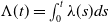 $\Lambda(t)=\int_{0}^{t}\lambda (s)ds$
for
 $t\geq 0$
, would represent the realized survival probability over [0,
 $T$
]. Since
 $e^{-\Lambda (T)}$
could theoretically exceed 1 due to the possibility of large negative jumps in the mortality rate process, we redefine the realized survival probability at maturity
 $T$
as
 $e^{-\Lambda _{0}(T)}$
, where
 $\Lambda _{0}(T)=\max \left\{\Lambda (T),0\right\} $
. Nevertheless, in our specific model, the probability of
 $e^{-\Lambda (T)}$
exceeding 1 is extremely low, so in practice,
 $\Lambda _{0}(T)=\Lambda (T)$
, making this adjustment just a theoretical safeguard.
For compactness, given
 $0\leq x_{\min }\leq x_{\max }\leq \infty $
and
 $x\in\mathbb{R}$
, we define the two-sided truncation of
 $x$
as
 $(x)_{x_{\min},x_{\max }}=\min \left\{ \max \left\{ x,x_{\min }\right\} ,x_{\max}\right\} $
. In particular,
 $\Lambda _{0}(T)=(\Lambda (T))_{0,\infty }$
.
We now introduce various payoff structures to be considered:
-
• S-forward: The payoff at maturity is given by
This can be interpreted as
\begin{equation*}C=a(e^{-\Lambda _{0}(T)}-b),\qquad a\gt0,b\in (0,1).\end{equation*}
$a$
units of a zero coupon swap, where a fixed survival probability
$b$
is exchanged for the realized survival probability
$e^{-\Lambda _{0}(T)}$
at maturity
$T$
. This derivative provides a hedge against the risk of a specified population deviating from a reference survival probability. For example, a pension fund or an insurance company facing longevity risk might agree to pay a fixed amount based on an initially expected survival rate. In return, the counterparty would pay a variable amount determined by the actual observed survival rates over the term of the contract. S-forward contracts have been extensively studied in the actuarial literature; see, for example, Bravo and Nunes (Reference Bravo and Nunes2021), Tang and Li (Reference Tang and Li2021), and Zeddouk and Devolder (Reference Zeddouk and Devolder2024).
-
• Longevity caplet: The payoff at maturity is given by
This is an option-type longevity derivative that pays
\begin{equation*}C=a(e^{-\Lambda _{0}(T)}-b)_{0,\infty },\qquad a\gt0,b\in (0,1).\end{equation*}
$a(e^{-\Lambda_{0}(T)}-b)$
if the realized survival probability
$e^{-\Lambda _{0}(T)}$
at maturity
$T$
exceeds a prespecified cap rate
$b$
, and zero otherwise. Unlike an S-forward, this derivative triggers a payoff only if the realized survival rate at maturity exceeds the threshold
$b$
. This payoff structure may be more appealing to insurers, as it transfers only extreme longevity risk and thus reduces the capital requirement. See Bauer et al. (Reference Bauer, Börger and Ruß2010) and Bravo and Nunes (Reference Bravo and Nunes2021) for related discussions.
-
• Unit-linked security: The payoff at maturity is given by
where
\begin{equation*}C=1_{(e^{-\Lambda _{0}(T)}\gt b)}(S(T))_{G_{\min },G_{\max }},\qquad b\in (0,1),\end{equation*}
$0\leq G_{\min }\lt G_{\max }\leq \infty $
represent the minimum and maximum guaranteed amounts provided by the contract issuer, respectively, and
$S$
(
$T$
) is the terminal value of a stock price. This investment-linked payout ensures that if the reference survival probability exceeds an agreed threshold
$b$
, the contract holder is paid based on the stock price at terminal
$T$
, subject to minimum and maximum guarantees. The unit-linked security provides protection against both extreme longevity risk and financial market downside risk—an idea akin to the hybrid catastrophe bonds concept proposed by Barrieu and Loubergé (Reference Barrieu and Loubergé2009). Given potential interactions between mortality outcomes and market performance, this dual protection feature could increase demand for the security. By the way, it is easy to see that (4.1)
\begin{equation}C=\underbrace{1_{(e^{-\Lambda _{0}(T)}\gt b)}G_{\min }}_{\text{guaranteed portion}}+\underbrace{1_{(e^{-\Lambda _{0}(T)}\gt b)}(S(T)-G_{\min})_{0,G_{\max }-G_{\min }}}_{\text{liability portion}}. \end{equation}


4.2. Dynamics of the asset price and mortality rate
Introduce a three-dimensional standard Brownian motion
 $\{\boldsymbol{W}(t)\}_{0\leq t\leq T}$
, to be used to model the dynamics of the risky asset price and mortality rate. As mentioned earlier, we consider a financial market consisting of a risk-free asset paying no interest and a risky asset. Suppose that the price per share of the risky asset, denoted by
 $\{S(t)\}_{0\leq t\leq T}$
, follows the stochastic volatility model, for
 $t\in \lbrack 0,T]$
,
 \begin{align}\frac{dS(t)}{S(t)} & = \mu dt+\Sigma (t)d\boldsymbol{W}(t), \nonumber\\\Sigma (t) & = (v(t))_{v_{\min },v_{\max }}^{0.5}\left( \rho ,\sqrt{1-\rho^{2}}\psi ,\sqrt{1-\rho ^{2}}\sqrt{1-\psi ^{2}}\right) , \end{align}
 \begin{align} dv(t) &=(\beta _{0}+\beta _{1}v(t))dt+{\sigma _{v}}(v(t))_{v_{\min},v_{\max }}^{\gamma }dW_{2}(t), \end{align}
where
 $\mu ,\beta _{0},\beta _{1}\in \mathbb{R}$
,
 ${\sigma _{v},}\gamma \gt0$
,
 $\rho ,\psi \in ({-}1,1)$
,
 $0 \lt v_{\min }\lt v_{\max }\lt \infty $
, and
 $S(0),v(0)\gt0$
are all constants. The existence of a unique solution to (4.3) is evident, as the volatility function
 ${\sigma _{v}(}v)_{{v_{\min }},v_{\max}}^{\gamma }$
, due to the two-sided truncation, is Lipschitz continuous. This stochastic volatility model is a slightly modified version of model (3) in Jones (Reference Jones2003), who, in studying the dynamic behavior of the volatility of equity index returns, proposes a generalization of the Heston model to incorporate a time-varying leverage effect on the instantaneous variance. It is common practice in financial modeling to employ truncation on the volatility process; for related discussions, see, for example, Appendix B of Davydov and Linetsky (Reference Davydov and Linetsky2001).
We assume that the reference mortality rate process
 $\{\lambda (t)\}_{0\leq t\leq T}$
evolves according to
 \begin{equation}d\lambda (t)=(a_{0}+a_{1}\lambda (t))dt+\sigma _{\lambda}dW_{1}(t)+d\sum_{i=1}^{N(t)}J_{i},\qquad t\in \left[ 0,T\right] ,\end{equation}
where
 $a_{0},a_{1}\in \mathbb{R}$
and
 $\sigma _{\lambda }$
 $\gt0$
are constants,
 $\{N(t)\}_{0\leq t\leq T}$
is a Poisson process with constant intensity
 ${\delta }\gt0$
, and
 $\{J_{i}\}_{i=1}^{\infty }$
is a sequence of independent and identically distributed jumps. Further assume that these jumps follow a common asymmetric double exponential distribution, with probability density function
 \begin{equation}\frac{\phi }{\varepsilon _{1}}e^{-u/\varepsilon _{1}}1_{(u\geq 0)}+\frac{1-\phi }{\varepsilon _{2}}e^{u/\varepsilon _{2}}1_{(u\lt0)},\qquad u\in\mathbb{R}, \end{equation}
for
 $\varepsilon _{1},\varepsilon _{2}\gt0$
and
 $\phi \in \lbrack 0,1]$
. As usual, assume that
 $\{\boldsymbol{W}(t)\}_{0\leq t\leq T}$
,
 $\{N(t)\}_{0\leq t\leq T}$
, and
 $\{J_{i}\}_{i=1}^{\infty }$
are mutually independent.
Notably, the reference mortality process
 $\{\lambda (t)\}_{0\leq t\leq T}$
and the asset price process
 $\{S(t)\}_{0\leq t\leq T}$
are allowed to be dependent, with the instantaneous correlation
 \begin{align*}\mathrm{corr}\left( \frac{dS(t)}{S(t)},d\lambda (t)\right) =\rho \frac{E\left[ \sqrt{(v(t))_{v_{\min },v_{\max }}(a_{0}+a_{1}\lambda (t))}\right] }{\sqrt{E[(v(t))_{v_{\min },v_{\max }}](E\left[ a_{0}+a_{1}\lambda (t)\right]+\delta E\left[ J^{2}\right] )}}.\end{align*}
Furthermore, we suppose that the set of admissible strategies consists of all real-valued and
 $\mathbb{F}$
predictable processes with values in the interval
 $\left[ \pi _{\min },{\pi _{\max }}\right] $
, where
 $-\infty \lt\pi_{\min }\lt\pi _{\max }\lt\infty $
.
4.3. Numerical approximation of the utility indifference price
To obtain the utility indifference price
 $p$
in (2.7) for an MLS, we need the values of
 $V$
(0,1) and
 $V$
(0,0). By Theorem 3.1, calculating these values reduces to evaluating
 $-e^{\alpha Y(0)}$
with
 $C$
set to the security’s payoff and
 $C=0$
, respectively. Alternatively, we can evaluate
 $-\tilde{Y}(0)$
, where
 $\{\tilde{Y}(t)\}_{0\leq t\leq T}$
corresponds to the auxiliary BSDE (A.1). We estimate the price
 $p$
using this alternative approach and numerically solve the auxiliary BSDE (A.1) to approximate
 $-\tilde{Y}(0)$
. The reason for following this approach is that discrete-time approximations for forward-BSDEs typically require the generator of the BSDE to be Lipschitz continuous; see Section 1 of Bouchard and Elie (Reference Bouchard and Elie2008).
The asset price process
 $\{S(t)\}_{0\leq t\leq T}$
described in (4.2) does not contain jumps, which implies that, under the general formula (2.1),
 $\theta (t,x)=0$
a.e. with respect to
 $dP\mathcal{\otimes }d\eta \mathcal{\otimes }dt$
. Thus, (A.1) simplifies to
 \begin{eqnarray}\tilde{Y}(t) &=&e^{\alpha C}+\int_{t}^{T}\left\{ -\alpha \pi _{\ast}(s)\left( \mu \tilde{Y}(s)+\Sigma (s){\tilde{\boldsymbol{Z}}}(s)\right) +\frac{1}{2}\alpha ^{2}\pi _{\ast }^{2}(s)\left\Vert \Sigma (s)\right\Vert ^{2}\tilde{Y}(s)\right\} ds \notag \\[7pt]&&-\int_{t}^{T}{\tilde{\boldsymbol{Z}}}^{\intercal }(s)d\boldsymbol{W}(s)-\int_{t}^{T}\int_{\mathbb{R}}\tilde{K}(s,x)\tilde{N}(ds,dx),\qquad t\in\lbrack 0,T], \end{eqnarray}
where
 \begin{equation*}\pi _{\ast }(t)=\left( \frac{1}{\alpha }\left\Vert \Sigma (t)\right\Vert ^{-2}\left( \mu +\Sigma (t)\tilde{\boldsymbol{Z}}(t)(\tilde{Y}(t))^{-1}\right) \right) _{\pi _{\min },\pi _{\max }}.\end{equation*}
We now describe a discrete-time approximation for the forward-BSDEs (4.2)–(4.6). This approximation is then implemented using an LSMC algorithm.
For every
 $t\in \lbrack 0,T]$
, define
 $\boldsymbol{\chi }(t)=\left(S(t),v(t),\lambda (t),\Lambda (t)\right) ^{\intercal }$
, where
 $S$
(
 $t$
),
 $v$
(
 $t$
), and
 $\lambda (t)$
are given by equations (4.2)–(4.4), respectively, and
 $\Lambda(t)=\int_{0}^{t}\lambda (s)ds$
. Let
 $0=t_{0}\lt t_{1}\lt \ldots \lt t_{m_{p}}=T$
be a partition of [0,
 $T$
] with an equal spacing of
 $h=\frac{T}{m_{p}}$
. A discrete-time approximation of
 $\{\boldsymbol{\chi }(t)\}_{0\leq t\leq T}$
, denoted by
 $\{\boldsymbol{\chi }_{h}(t)\}_{0\leq t\leq T}$
 $=\{\left(S_{h}(t),v_{h}(t),\lambda _{h}(t),\Lambda _{h}(t)\right) ^{\intercal}\}_{0\leq t\leq T}$
, is given by the Euler scheme. Consider a payoff of the form
 $C=c(\boldsymbol{\chi }(T))$
, where
 $c(\!\cdot\!)$
is a real-valued and bounded measurable function. Given the approximation
 $\{\boldsymbol{\chi }_{h}(t)\}_{0\leq t\leq T}$
, an approximated solution
 $( \tilde{Y}_{h}(t),{\tilde{\boldsymbol{Z}}}_{h}(t)) _{0\leq t\leq T}$
to the BSDE (4.6) is given by the backward recursion
 \begin{equation*}\left\{\begin{array}{l}\displaystyle\tilde{Y}_{h}(T)=e^{\alpha c(\boldsymbol{\chi }_{h}(T))}, \\[8pt] \displaystyle {\tilde{\boldsymbol{Z}}}_{h}(t_{i})=\frac{1}{h}E\left[ \left. \tilde{Y}_{h}(t_{i+1})\left( \boldsymbol{W}(t_{i+1})-\boldsymbol{W}(t_{i})\right)\right\vert \mathcal{F}_{t_{i}}\right] , \\[12pt] \displaystyle \tilde{Y}_{h}(t_{i})=E\big[ \tilde{Y}_{h}(t_{i+1})+g\big(\boldsymbol{\chi }_{h}(t_{i}),\tilde{Y}_{h}(t_{i+1}),{\tilde{\boldsymbol{Z}}}_{h}(t_{i})\big) h\big\vert \mathcal{F}_{t_{i}}\big] ,\end{array}\right.\end{equation*}
and
 $( \tilde{Y}_{h}(t),{\tilde{\boldsymbol{Z}}}_{h}(t)) =(\tilde{Y}_{h}(t_{i}),{\tilde{\boldsymbol{Z}}}_{h}(t_{i})) $
for
 $t_{i}\leq t\lt t_{i+1}$
, where
 $i=0,\ldots ,m_{p}-1$
and
 $g(\!\cdot\!)$
corresponds to the generator of (4.6). The conditional expectations are approximated using the LSMC method with four sets of
 $m_{b}$
dimensional basis functions,
 $\boldsymbol{b}_{l}(\!\cdot\!)=\left( b_{l,1}(\!\cdot\!),\ldots,b_{l,m_{b}}(\!\cdot\!)\right) ^{\intercal }$
for
 $l=0,1,2,3$
; see Longstaff and Schwartz (Reference Longstaff and Schwartz2001).
We now describe how to simulate
 $m_{s}$
sample paths of
 $\{\tilde{Y}(t)\}_{0\leq t\leq T}$
using the LSMC algorithm. To facilitate the description, we define three independent random objects:
-
• a three-dimensional normal random vector
$\Delta \boldsymbol{W}_{h}$
with independent components, each having mean 0 and variance
$h\gt0$
; -
• a random variable
$\Delta N_{h}$
following a Poisson distribution with mean
${\delta }h$
; -
• a random variable
$J$
following an asymmetric double exponential distribution (4.5) with parameters
$(\varepsilon _{1},\varepsilon_{2},\phi )$
.


We apply the LSMC algorithm according to the following steps:
-
1. Simulate
$m_{p}\times m_{s}$
independent copies of
$\Delta \boldsymbol{W}_{h}$
and
$\Delta N_{h}$
and store them in
$\Delta \boldsymbol{W}^{j}(i+1) $
and
$\Delta N^{j}(i+1)$
, respectively, for
$i=0,\ldots ,m_{p}-1$
and
$j=1,\ldots ,m_{s}$
. Then, simulate
$\Delta N^{j}(i+1)$
independent copies of
$J$
for
$i=0,\ldots ,m_{p}-1$
and
$j=1,\ldots ,m_{s}$
. -
2. Generate
$m_{s}$
independent copies of
$\left\{ \boldsymbol{\chi }_{h}(t_{i})\right\} _{i=1}^{m_{p}}$
according to the Euler scheme and store them in
$\{\boldsymbol{\chi }_{h}^{j}(t_{i})\}_{i=1}^{m_{p}}$
for
$j=1,\ldots,m_{s}$
. -
3. Set
$\hat{Y}\left( T,\boldsymbol{\chi }_{h}^{j}(T)\right) =e^{\alpha c(\boldsymbol{\chi }_{h}^{j}(T))}$
for
$j=1,\ldots ,m_{s}$
. -
4. For
$i=0,\ldots ,m_{p}-1$
,-
(a) solve the least-squares regression
and set
\begin{equation*}\boldsymbol{\xi }_{l}=\mathop{\mathrm{arg\,min}}\limits_{\boldsymbol{\xi }\in \mathbb{R}^{m_{b}}}\left\{ \frac{1}{m_{s}}\sum_{j=1}^{m_{s}}\left\vert \frac{1}{h}\hat{Y}\left( t_{i+1},\boldsymbol{\chi }_{h}^{j}(t_{i+1})\right) \Delta W_{l}^{j}(i+1)-\boldsymbol{\xi }^{\intercal }\boldsymbol{b}_{l}\left(\boldsymbol{\chi }_{h}^{j}(t_{i})\right) \right\vert ^{2}\right\}\end{equation*}
$\hat{Z}_{l}\left( t_{i},\boldsymbol{\chi }_{h}^{j}(t_{i})\right) =\boldsymbol{\xi }_{l}^{\top }\boldsymbol{b}_{l}\left( \boldsymbol{\chi }_{h}^{j}(t_{i})\right) $
for
$l=1,2,3$
and
$j=1,\ldots ,m_{s}$
;
-
(b) solve the least-squares regression
and set
\begin{eqnarray*}\boldsymbol{\xi }_{0} &=&\mathop{\mathrm{arg\,min}}\limits_{\boldsymbol{\xi }\in \mathbb{R}^{m_{b}}}\left\{ \frac{1}{m_{s}}\sum_{j=1}^{m_{s}}\left\vert \hat{Y}\left(t_{i+1},\boldsymbol{\chi }_{h}^{j}(t_{i+1})\right) \right. \right. \\&&\left. \left. +g\left( \boldsymbol{\chi }_{h}^{j}(t_{i}),\hat{Y}\left(t_{i+1},\boldsymbol{\chi }_{h}^{j}(t_{i+1})\right) ,{\hat{\boldsymbol{Z}}}\left( t_{i},\boldsymbol{\chi }_{h}^{j}(t_{i})\right) \right) h-\boldsymbol{\xi }^{\intercal }\boldsymbol{b}_{0}\left( \boldsymbol{\chi }_{h}^{j}(t_{i})\right) \vphantom{\tilde{Y}^{j}}\right\vert ^{2}\vphantom{\sum_{j=1}^{m}}\right\} ,\end{eqnarray*}
$\hat{Y}\left( t_{i},\boldsymbol{\chi }_{h}^{j}(t_{i})\right) =\boldsymbol{\xi }_{0}^{\intercal }\boldsymbol{b}_{0}\left( \boldsymbol{\chi }_{h}^{j}(t_{i})\right) $
and
$j=1,\ldots ,m_{s}$
.
-


The procedure above yields approximated sample paths for the solution
 $\{\tilde{Y}(t)\}_{0\leq t\leq T}$
of the auxiliary BSDE (A.1) with
 $C $
equal to the payoff of the security. We then set
 $V(0,1)=-\tilde{Y}(0)$
. The procedure is repeated using the same process with
 $C=0$
to generate sample paths of
 $\{\tilde{Y}(t)\}_{0\leq t\leq T}$
, which results in the estimate
 $V(0,0)=-\tilde{Y}(0)$
. The utility indifference price of the contract at
 $t=0$
is then obtained by plugging these values to (2.7).
4.4. Implementation and results
In our numerical studies, we compute the indifference prices of the three MLSs introduced earlier in Subsection 4.1: S-forward, longevity caplet, and unit-linked security. Specifically, we illustrate the impact of the mortality rate parameters, the correlation parameter, and short-selling constraints on these indifference prices. Our results demonstrate that the parameters of the mortality rate, particularly the drift coefficient
 $a_{1}$
and the jump intensity
 $\delta $
, have a more pronounced effect on pricing than those governing the asset price dynamics. Furthermore, the correlation between the risky asset price and the mortality rate significantly influences pricing, especially for unit-linked securities.
Baseline estimation
For the mortality rate in (4.4), we use the parameters calibrated by Bravo and Nunes (Reference Bravo and Nunes2021), based on annual mortality data from 1950 to 2017 for the total US population aged 65 years in 1990. For the price process of the risky asset described by (4.2)–(4.3), we estimate its parameters using daily closing prices of the S&P 500 index from 2005 to 2017, employing the SVDNF package in R (Arsenault-Mahjoubi et al., Reference Arsenault-Mahjoubi, Bégin and Boudreault2024). This ensures using time windows with the same ending year when estimating parameters for the asset price and mortality rate models. We refrain from a full joint re-estimation of both models due to the mismatch in data frequencies—mortality data are annual, while stock price data are daily.
For the three MLSs, we consider a time horizon
 $T=10$
. The absolute risk aversion parameter
 $\alpha $
in (2.4) is set to
 $0.02$
, which falls within the range of absolute risk aversion estimates surveyed by Babcock et al. (Reference Babcock, Choi and Feinerman1993). The values of
 $b$
and
 $G_{\min }$
are set to the median of the simulated values of
 $e^{-\Lambda _{0}(T)}$
and
 $S$
(
 $T$
), respectively, indicating that the survival probability threshold and the minimum guarantee reasonably reflect expectations of future values of reference survival probabilities and asset price values. The initial values
 $S(0)$
and
 $v$
(0) and the parameters
 $a$
,
 $G_{\max }$
,
 $v_{\min }$
,
 $v_{\max} $
,
 $\pi _{\min }$
, and
 $\pi _{\max }$
are set to arbitrary but reasonable values. In particular, the values of
 $\pi _{\min }$
and
 $\pi _{\max }$
are set far from 0 to ensure that they have virtually no impact on pricing. The number of partitions
 $m_{p}$
and the number of simulations
 $m_{s}$
are set to 150 and 25,000, respectively. In the LSMC implementation, we use Laguerre polynomials of degree up to
 $m_{b}=2$
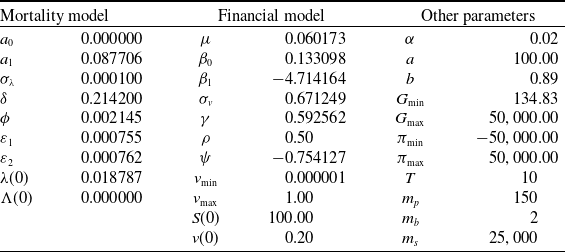
as basis functions for each state variable. The choice of basis functions can be adjusted without significant impact on the results; see Longstaff and Schwartz (Reference Longstaff and Schwartz2001). Table 2 collects all the parameter values used in the baseline investigation.
Parameters used for the base numerical experiments.

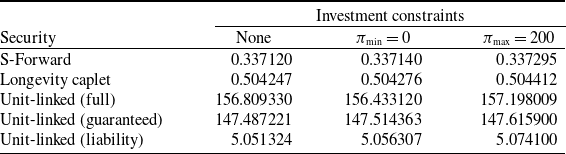
The first set of results, shown in Table 3, illustrates the impact of portfolio constraints on the indifference prices of the three MLSs we consider. Regarding the unit-linked security, we report the prices of three payoffs: one for the full payoff
 $C$
on the left-hand side of (4.1) and the other two for the guaranteed and liability portions from the decomposition on the right-hand side of (4.1). From these results, we find that imposing a short-selling restriction (
 $\pi _{\min }=0$
) or an upper investment constraint (
 $\pi_{\max }=200$
) has little to no impact on the indifference prices.
Indifference prices for the mortality- and unit-linked securities with and without investment constraints.

Notably, the results in the last three rows indicate that the indifference prices for the three payoffs related to the unit-linked security satisfy super-additivity, though this has not been established in a general context. We also note that, although the mortality rate model includes jumps, the parameter estimates do not account for the mortality shocks caused by the COVID-19 pandemic. Nevertheless, we conduct a sensitivity analysis of the indifference prices, with particular attention to the jump intensity
 $\delta$
of the mortality rate process.
Sensitivity analysis
We now conduct a sensitivity test of indifference prices against various key parameters in the mortality rate and asset price models, including the correlation parameter
 $\rho $
, the jump intensity
 $\delta $
and the drift
 $a_{1}$
of the mortality rate, the expected rate of return
 $\mu $
, and the drift
 $\beta _{1}$
of the volatility process. Additionally, we consider the absolute risk aversion parameter
 $\alpha $
in (2.4). The ranges for some of these parameters are
 $\rho \in (-1,1)$
,
 $\delta \in \lbrack 0,2]$
, and
 $\alpha \in (0,0.03]$
, while the other parameters
 $a_{1}$
,
 $\mu $
, and
 $\beta _{1}$
vary within
 $\pm 10\%$
of their baseline values listed in Table 2.
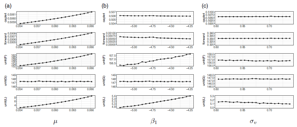
The results of the sensitivity analysis are visualized in Figure 1. To supplement the visual analysis, we compute the arc elasticities of the indifference prices with respect to the model parameters using the following formula:
 \begin{equation*}\text{arc-elasticity}=\left\vert \frac{y_{2}-y_{1}}{\frac{1}{2}(y_{1}+y_{2})}\cdot \frac{\frac{1}{2}(x_{1}+x_{2})}{x_{2}-x_{1}}\right\vert ,\end{equation*}
where
 $x_{1},x_{2}$
represent the values of a specific parameter under consideration, and
 $y_{1},y_{2}$
the resulting indifference prices.
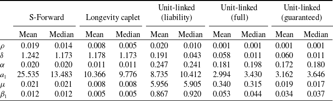
The arc elasticities are computed for each adjacent pair of parameter values and indifference prices. In Table 4, we report the mean and median arc elasticity for each security with respect to each parameter under consideration. These are regarded as measures of central tendency due to the occurrence of outliers, particularly when the parameter value changes from a value close to zero. Since the elasticities are, by definition, nonnegative, the overall direction of the impact can be gleaned from Figure 1.
Arc elasticities of indifference prices with respect to various key mortality and financial parameters.

Indifference prices for various values of key mortality and financial parameters.

For the S-forward and longevity caplet derivatives, whose payoffs depend solely on the mortality rate, the indifference prices are primarily influenced by mortality rate parameters, with financial model parameters having a “second-order” effect. This is evident from the relatively high (median) elasticities with respect to the mortality rate parameters
 $\delta $
and
 $a_{1}$
, compared to other parameters in the asset price model. Moreover, the indifference prices of these instruments exhibit mild elasticity with respect to
 $\rho $
.
In contrast, for the unit-linked security, the effect of mortality shocks is less pronounced, as indicated by the elasticities with respect to
 $\delta $
. Furthermore, the indifference prices corresponding to the unit-linked security, particularly the liability portion, are more sensitive to changes in
 $\rho $
.
The S-forward and longevity caplet are both highly elastic with respect to changes in the jump intensity
 $\delta $
of the mortality rate process. As
 $\delta $
increases, the likelihood of jumps in the mortality process rises, which in turn boosts the payoff. In contrast, the indifference price of the unit-linked security exhibits a less straightforward relationship with
 $\delta $
, exhibiting an upward trend that slows at higher levels of
 $\delta $
.
Apparently, the indifference prices of all three securities increase with the coefficient of absolute risk aversion
 $\alpha $
. The issuer, when becoming more risk-averse, demands a higher price to issue a contract to the buyer.
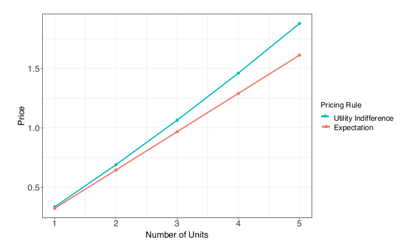
In Appendix A.3, we show that the performance of financial assets, even when assumed to be independent of the mortality rate, still influences the pricing of mortality derivatives.
In the baseline case, the mortality rate process
 $\{\lambda (t)\}_{0\leq t\leq T}$
is not mean-reverting since
 $a_{1}\gt0$
. This implies that, in the long run, its continuous part exhibits an upward trend, with a higher
 $a_{1}$
indicating a faster rate of increase. Our numerical experiments show that the indifference prices of the longevity caplet and the S-forward are highly sensitive to changes in
 $a_{1}$
. These prices decrease as
 $a_{1}$
increases because, as the mortality rate rises over time, the payoff declines, leading the issuer to demand a lower price. For the unit-linked security, a higher mortality rate reduces the likelihood of a payoff, and thus its price also tends to decrease with
 $a_{1}$
, though the effect is less significant than for the longevity caplet and the S-forward.
5. Concluding remarks
This paper explores the pricing of a general MLS, where the mortality rate and asset prices jointly follow a multivariate Itô process with jumps. The proposed pricing framework follows the utility indifference approach and leverages BSDE techniques. Numerical studies demonstrate its effectiveness in capturing the impacts of various parameters governing the mortality rate and asset prices, with a particular focus on their correlation.
We acknowledge several limitations of the present research. In our theoretical development, we assume that the coefficients of the Itô process, the admissible strategies, and the payoff are bounded. Allowing any of these to be unbounded would introduce significant technical complexities. We adopt exponential utility, which greatly simplifies the utility indifference analysis. Extending our work to other non-exponential utility functions would require substantial changes. Additionally, we consider a single payoff occurring at maturity, whereas most financial instruments involve a series of payments (e.g., coupon and principal payments). This would require developing the pricing framework in a multistage setting. Most critically, the payoff is assumed to depend only on the history of the mortality rate and asset prices. In practice, however, other risk factors—such as the issuer’s default risk, the buyer’s surrender risk, market liquidity risk, and broader economic conditions—may significantly affect the price. These additional risk factors would require advanced techniques such as filtration enlargement to address. Extensions in these directions are practically relevant but theoretically challenging, and they warrant further research.
Acknowledgments
The authors thank two anonymous referees and Editor Łukasz Delong for their helpful comments on earlier versions of this paper. Garces acknowledges support from the Australian Research Council Centre of Excellence in Population Ageing (CE170100005). Gómez acknowledges support from the UNSW’s SHARP Fund for Postdoctoral Fellowships. Tang acknowledges support from the Australian Government through the Australian Research Council’s Discovery Projects funding scheme (DP200101859, DP220100090, and DP250100078).
Appendix A
Appendix A.1 presents the proof of Theorem 3.1, Appendix A.2 collects auxiliary derivations required for the proof, and Appendix A.3 provides additional clarifying comments.
A.1. Proof of Theorem 3.1
We will apply Itô’s lemma for semimartingales multiple times, and follow the complete version given in Theorem 5.1 in Chapter II of Ikeda and Watanabe (Reference Ikeda and Watanabe1981).
(i) This proof builds on Lemma 2.4 from Tang and Li (Reference Tang and Li1994), which establishes the existence and uniqueness of solutions to BSDEs with a Lipschitz generator. Specifically, we manage to connect the BSDE (3.4) to the one considered in Lemma 2.4 of Tang and Li (Reference Tang and Li1994).
We begin by proving the uniqueness of the solution to the BSDE (3.4). Assume that
 $(Y,\boldsymbol{Z},K)\in \mathcal{S}^{\infty}\times \mathcal{L}^{2,m}\times \mathcal{L}_{\eta }^{2}$
solves (3.4). For
 $t\in \left[ 0,T\right] $
, we make the changes of variables
 \begin{equation*}\left\{\begin{array}{l}\displaystyle\tilde{Y}(t)=e^{\alpha Y(t)},\\[4pt]\displaystyle{\tilde{\boldsymbol{Z}}}(t)=\alpha \tilde{Y}(t)\boldsymbol{Z}(t), \\[4pt]\displaystyle\tilde{K}(t,\cdot )=\tilde{Y}(t-)\left( e^{\alpha K(t,\cdot )}-1\right) .\end{array}\right.\end{equation*}
By Itô’s lemma, we can show that
 $( \tilde{Y}(t),{{\tilde{\boldsymbol{Z}}}}(t),\tilde{K}(t)) _{0\leq t\leq T}$
satisfies the BSDE
 \begin{eqnarray}\tilde{Y}(t) &=&e^{\alpha C}+\int_{t}^{T}\mathop{\mathrm{ess\,inf}}\limits_{\boldsymbol{\pi }\in\mathcal{A}}\, \{ g^{\boldsymbol{\pi }}( s,\tilde{Y}(s),{\tilde{\boldsymbol{Z}}}(s),\tilde{K}(s,\cdot )) \} ds \notag \\[4pt]&&-\int_{t}^{T}{\tilde{\boldsymbol{Z}}}^{\intercal }(s)d\boldsymbol{W}(s)-\int_{t}^{T}\int_{\mathbb{R}^{n}}\tilde{K}(s,\boldsymbol{x})\tilde{N}(ds,d\boldsymbol{x}), \end{eqnarray}
where, for every
 $(s,y,\boldsymbol{z},k)\in \left[ 0,T\right] \times \mathbb{R}\times \mathbb{R}^{m}\times H_{\eta }^{2}$
and
 $\boldsymbol{\pi }\in\mathcal{A}$
,
 \begin{eqnarray}g^{\boldsymbol{\pi }}(s,y,\boldsymbol{z},k) &=&-\alpha \boldsymbol{\pi }^{\intercal }(s)\left( \boldsymbol{\mu }(s)y+\Sigma (s)\boldsymbol{z}\right)+\frac{1}{2}\alpha ^{2}\left\Vert \boldsymbol{\pi }^{\intercal }(s)\Sigma(s)\right\Vert ^{2}y \notag \\[4pt]&&+\int_{\mathbb{R}^{n}}\left( e^{-\alpha \boldsymbol{\pi }^{\intercal }(s)\boldsymbol{\theta }(s,\boldsymbol{x})}-1\right) k(\boldsymbol{x})\eta (d\boldsymbol{x}) \notag \\[4pt]&&+\int_{\mathbb{R}^{n}}\left( \alpha \boldsymbol{\pi }^{\intercal }(s)\boldsymbol{\theta }(s,\boldsymbol{x})+e^{-\alpha \boldsymbol{\pi }^{\intercal }(s)\boldsymbol{\theta }(s,\boldsymbol{x})}-1\right) \eta (d\boldsymbol{x})y. \end{eqnarray}
See Appendix A.2.1 for a detailed derivation. Based on this relationship, we reduce the analysis of (3.4) to that of (A.1).
With
 $s\in \left[ 0,T\right] $
fixed, define
 \begin{equation}g(s,y,\boldsymbol{z},k)=\mathop{\mathrm{ess\,inf}}\limits_{\boldsymbol{\pi }\in \mathcal{A}}\left\{g^{\boldsymbol{\pi }}(s,y,\boldsymbol{z},k) \right\},\qquad (y,\boldsymbol{z},k)\in\mathbb{R}\times \mathbb{R}^{m}\times H_{\eta }^{2}. \end{equation}
Since
 $\left\{ g^{\boldsymbol{\pi }}(\!\cdot\!)\right\} _{\boldsymbol{\pi }\in\mathcal{A}}$
is a collection of Lipschitz continuous functions sharing a common Lipschitz constant, and the strategies in
 $\mathcal{A}$
are bounded, the infimum of this family over
 $\boldsymbol{\pi }\in \mathcal{A}$
, denoted
 $g(\!\cdot\!)$
, is also a Lipschitz continuous function with the same Lipschitz constant; see, for example, Proposition 1.32 of Weaver (Reference Weaver2018). According to Lemma 2.4 of Tang and Li (Reference Tang and Li1994), there exists a unique solution
 $(\tilde{Y}_{1},{\tilde{\boldsymbol{Z}}}_{1},\tilde{K}_{1})\in \mathcal{S}^{2}\times \mathcal{L}^{2,m}\times \mathcal{L}_{\eta }^{2}$
to the BSDE (A.1), which implies that
 $(Y,\boldsymbol{Z},K)\in \mathcal{S}^{\infty}\times \mathcal{L}^{2,m}\times \mathcal{L}_{\eta }^{2}$
uniquely solves (3.4).
We now proceed to establish the existence of a solution to (3.4). Let
 $(\tilde{Y},{\tilde{\boldsymbol{Z}}},\tilde{K})\in \mathcal{S}^{2}\times\mathcal{L}^{2,m}\times \mathcal{L}_{\eta }^{2}$
be the unique solution to the BSDE (A.1). By employing a measurable selection argument similar to Lemma 11 of Hu et al. (Reference Hu, Imkeller and Müller2005) and Lemma 5.5 of Quenez and Sulem (Reference Quenez and Sulem2013), there exists a strategy
 $\left\{ \boldsymbol{\pi }_{\ast}(t)\right\} _{0\leq t\leq T}$
satisfying, a.e. with respect to
 $dP\mathcal{\otimes }dt$
,
 \begin{equation*}g( t,\tilde{Y}(t),{\tilde{\boldsymbol{Z}}}(t),\tilde{K}(t,\cdot ))=g^{\boldsymbol{\pi }_{\ast }}( t,\tilde{Y}(t),{\tilde{\boldsymbol{Z}}}(t),\tilde{K}(t,\cdot )) .\end{equation*}
By Theorem 3.4 of Quenez and Sulem (Reference Quenez and Sulem2013), we can show that
 $\{\tilde{Y}(t)\}_{0\leq t\leq T}$
has the representation
 \begin{eqnarray}\tilde{Y}(t) &=&E^{Q}\left[ \exp \left\{ \alpha C+\int_{t}^{T}\left( \vphantom{\int}-\alpha \boldsymbol{\pi }_{\ast }^{\intercal }(s)\boldsymbol{\mu }(s)+\frac{1}{2}\alpha ^{2}\left\Vert \boldsymbol{\pi }_{\ast}^{\intercal }(s)\Sigma (s)\right\Vert ^{2}\right. \right. \right. \notag \\&&\left. \left. \left. \left. +\int_{\mathbb{R}^{n}}\big( \alpha\boldsymbol{\pi }_{\ast }^{\intercal }(s)\boldsymbol{\theta }(s,\boldsymbol{x})+e^{-\alpha \boldsymbol{\pi }_{\ast }^{\intercal }(s)\boldsymbol{\theta }(s,\boldsymbol{x})}-1\big) \eta (d\boldsymbol{x})\right) ds\right\}\right\vert \mathcal{F}_{t}\right] , \end{eqnarray}
where the equivalent measure
 $Q$
is defined by
 \begin{equation}\frac{dQ}{dP}=\zeta (T), \end{equation}
with
 $\{\zeta (t)\}_{0\leq t\leq T}$
being the unique solution to
 \begin{equation}\left\{\begin{array}{l}\displaystyle\frac{d\zeta (t)}{\zeta (t-)}=-\alpha \boldsymbol{\pi }_{\ast }^{\intercal}(t)\Sigma (t)d\boldsymbol{W}(t)+\int_{\mathbb{R}^{n}}\big( e^{-\alpha\boldsymbol{\pi }_{\ast }^{\intercal }(t)\boldsymbol{\theta }(t,\boldsymbol{x})}-1\big) \tilde{N}(dt,d\boldsymbol{x}), \\[13pt]\displaystyle\zeta (0)=1.\end{array}\right. \end{equation}
See Appendix A.2.2 for a detailed explanation.
The representation (A.4) demonstrates that
 $\{\tilde{Y}(t)\}_{0\leq t\leq T}$
is strictly positive and bounded both above and away from zero. Consequently,
 $\{\tilde{K}(t,\boldsymbol{x})\}_{0\leq t\leq T,\boldsymbol{x}\in \mathbb{R}^{n}}$
, which constitutes the jump part of
 $\{\tilde{Y}(t)\}_{0\leq t\leq T}$
through (A.1), must also be bounded. For
 $t\in \left[ 0,T\right] $
, we introduce the transformation
 \begin{equation*}\left\{\begin{array}{l}\displaystyle Y(t)=\frac{1}{\alpha }\ln \tilde{Y}(t), \\[15pt]\boldsymbol{Z}(t)=\dfrac{1}{\alpha }\dfrac{{\tilde{\boldsymbol{Z}}}(t)}{\tilde{Y}(t)},\\[15pt]\displaystyle K(t,\cdot )=\frac{1}{\alpha }\ln \left( \frac{\tilde{K}(t,\cdot )}{\tilde{Y}(t-)}+1\right) .\end{array}\right.\end{equation*}
By using Itô’s formula again, we can show that the process
 $(Y,\boldsymbol{Z},K)\in \mathcal{S}^{\infty }\times \mathcal{L}^{2,m}\times \mathcal{L}_{\eta }^{2}$
satisfies the BSDE (3.4). The verification follows the same approach as in Appendix A.2.1. This proves the existence of a solution to the BSDE (3.4).
(ii) This proof consists of the following steps. We shall establish the existence of an admissible strategy
 $\boldsymbol{\pi }_{\ast }\in \mathcal{A}$
for the utility maximization problem in (2.5) with
 $w=0$
and
 $q=1$
by utilizing the construction outlined in (3.2) and (3.3). In doing so, we first introduce
 $f_{\ast }(\!\cdot\!)$
and
 $\left\{ \boldsymbol{\pi }_{\ast }(t)\right\} _{0\leq t\leq T}$
, as defined in (A.10) and (A.11) below, respectively. We then demonstrate that
 $\{R^{\boldsymbol{\pi }}(t)\}_{0\leq t\leq T}$
in (3.2), with generator
 $f_{\ast }(\!\cdot\!)$
, is a supermartingale for all
 $\boldsymbol{\pi }\in\mathcal{A}$
and
 $\{R^{\boldsymbol{\pi }_{\ast }}(t)\}_{0\leq t\leq T}$
is a martingale. From (3.1), we observe that the supremum in (2.5) is attained at
 $\left\{ \boldsymbol{\pi }_{\ast }(t)\right\}_{0\leq t\leq T}$
and that
 $V(0,1)=-e^{\alpha Y(0)}$
. Having established the existence of an optimal strategy
 $\boldsymbol{\pi }_{\ast }\in \mathcal{A}$
, we finally verify that attaining the infimum in (A.10) is a necessary condition for the optimality in (2.5).
For every
 $t\in \lbrack 0,T]$
and
 $\boldsymbol{\pi }\in \mathcal{A}$
, it follows from (2.3) and (3.3) that
 \begin{eqnarray*}&&-\alpha (X^{\boldsymbol{\pi }}(t)-Y(t)) \\&=&\alpha Y(0)-\alpha \int_{0}^{t}(\boldsymbol{\pi }^{\intercal }(s)\boldsymbol{\mu }(s)+f\left( s,Y(s),\boldsymbol{Z}(s),K(s,\cdot )\right)\!)ds\\&&-\alpha \int_{0}^{t}(\boldsymbol{\pi }^{\intercal }(s)\Sigma (s)-\boldsymbol{Z}^{\intercal }(s))d\boldsymbol{W}(s)-\alpha \int_{0}^{t}\int_{\mathbb{R}^{n}}(\boldsymbol{\pi }^{\intercal }(s)\boldsymbol{\theta }(s,\boldsymbol{x})-K(s,\boldsymbol{x}))\tilde{N}(ds,d\boldsymbol{x}).\end{eqnarray*}
Then by Itô’s lemma, we can prove that
 $\{R^{\boldsymbol{\pi }}(t)\}_{0\leq t\leq T}$
in (3.2) satisfies
 \begin{equation}\frac{dR^{\boldsymbol{\pi }}(t)}{R^{\boldsymbol{\pi }}(t-)}=d(M_{W}^{\boldsymbol{\pi }}(t)+M_{N}^{\boldsymbol{\pi }}(t))+dA^{\boldsymbol{\pi }}(t),\qquad t\in \lbrack 0,T],\boldsymbol{\pi }\in \mathcal{A},\end{equation}
where
 \begin{equation}\left\{\begin{array}{l}\displaystyle M_{W}^{\boldsymbol{\pi }}(t)=\int_{0}^{t}-\alpha (\boldsymbol{\pi }^{\intercal }(s)\Sigma (s)-\boldsymbol{Z}^{\intercal }(s))d\boldsymbol{W}(s), \\[14pt] \displaystyle M_{N}^{\boldsymbol{\pi }}(t)=\int_{0}^{t}\int_{\mathbb{R}^{n}}\left(e^{-\alpha (\boldsymbol{\pi }^{\intercal }(s)\boldsymbol{\theta }(s,\boldsymbol{x})-K(s,\boldsymbol{x}))}-1\right) \tilde{N}(ds,d\boldsymbol{x}), \\[14pt] \displaystyle A^{\boldsymbol{\pi }}(t)=\int_{0}^{t}(\!-\alpha f\left( s,Y(s),\boldsymbol{Z}(s),K(s,\cdot )\right) +\alpha f^{\boldsymbol{\pi }}\left( s,\boldsymbol{Z}(s),K(s,\cdot )\right) )ds,\end{array}\right. \end{equation}
and
 $f^{\boldsymbol{\pi }}(\!\cdot\!)$
is given in (3.5). Equivalently,
 \begin{equation*}R^{\boldsymbol{\pi }}(t)=\mathcal{E}\left\{ M_{W}^{\boldsymbol{\pi }}+M_{N}^{\boldsymbol{\pi }}+A^{\boldsymbol{\pi }}\right\} (t),\qquad t\in \lbrack0,T],\boldsymbol{\pi }\in \mathcal{A},\end{equation*}
where
 $\mathcal{E}$
denotes the stochastic exponential operator. For every
 $\boldsymbol{\pi }\in \mathcal{A}$
, by Theorem 38 in Chapter II of Protter (Reference Protter2005) with
 $X=M_{W}^{\boldsymbol{\pi }}+M_{N}^{\boldsymbol{\pi }}$
and
 $Y=A^{\boldsymbol{\pi }}$
, we obtain
 \begin{equation}R^{\boldsymbol{\pi }}(t)=R(0)M^{\boldsymbol{\pi }}(t)e^{A^{\boldsymbol{\pi }}(t)},\qquad t\in \lbrack 0,T],\boldsymbol{\pi }\in \mathcal{A},\end{equation}
where
 $M^{\boldsymbol{\pi }}(t)=\mathcal{E}\left\{ M_{W}^{\boldsymbol{\pi }}+M_{N}^{\boldsymbol{\pi }}\right\} (t)$
. Based on this representation, for
 $s\in \left[ 0,T\right] $
fixed, we introduce
 \begin{equation}f_{\ast }(s,\boldsymbol{z},k)=\mathop{\mathrm{ess\,inf}}\limits_{\boldsymbol{\pi }\in \mathcal{A}}\,\left\{f^{\boldsymbol{\pi }}(s,\boldsymbol{z},k) \right\},\qquad (\boldsymbol{z},k)\in \mathbb{R}^{m}\times H_{\eta }^{2}. \end{equation}
Subject to a measurable selection argument, we can find a strategy
 $\left\{\boldsymbol{\pi }_{\ast }(t)\right\} _{0\leq t\leq T}$
such that, a.e. with respect to
 $dP\mathcal{\otimes }dt$
,
 \begin{equation}f_{\ast }\left( t,\boldsymbol{Z}(t),K(t,\cdot )\right) =f^{\boldsymbol{\pi }_{\ast }}\left( t,\boldsymbol{Z}(t),K(t,\cdot )\right) . \end{equation}
Since
 $\{M^{\boldsymbol{\pi }}(t)\}_{0\leq t\leq T}$
is a positive local martingale for all
 $\boldsymbol{\pi }\in \mathcal{A}$
, there exists a sequence of stopping times
 $\left\{ \tau _{l}\right\} _{l\geq 1}$
, with
 $\tau _{l}\rightarrow T$
as
 $l\rightarrow \infty $
, such that
 $\left\{ M^{\boldsymbol{\pi }}(t\wedge \tau _{l})\right\} _{0\leq t\leq T}$
is a positive martingale. By
 $f_{\ast }(\!\cdot\!)$
in (A.10), the process
 $\{ e^{A^{\boldsymbol{\pi }}(t)}\} _{0\leq t\leq T}$
is nondecreasing. Consequently,
 $\left\{ R^{\boldsymbol{\pi }}(t\wedge \tau_{l})\right\} _{0\leq t\leq T}$
is a supermartingale; namely, it holds for every
 $s\leq t$
and
 $B\in \mathcal{F}_{s}$
that
 \begin{equation}E\left[ R^{\boldsymbol{\pi }}(t\wedge \tau _{l})1_{B}\right] \leq E\left[ R^{\boldsymbol{\pi }}(s\wedge \tau _{l})1_{B}\right] . \end{equation}
For each
 $\boldsymbol{\pi }\in \mathcal{A}$
, it is not difficult to see that the family
 $\left\{ -e^{-\alpha X^{\boldsymbol{\pi }}(\tau )}\,:\,\tau \text{ is an }\mathbb{F}\text{ stopping time}\right\}$
is uniformly integrable. The argument for this result proceeds along the same lines as the proof of Lemma 1 in Morlais (Reference Morlais2009). Moreover, since
 $Y$
is uniformly bounded, it follows that
 \begin{equation*}\left\{ R^{\boldsymbol{\pi }}(\tau )\,:\,\tau \text{ is an }\mathbb{F}\text{ stopping time}\right\}\end{equation*}
is uniformly integrable. Therefore, we can take the limit
 $l\rightarrow\infty $
in (A.12) to obtain the supermartingale property of
 $\{R^{\boldsymbol{\pi }}(t)\}_{0\leq t\leq T}$
. Since
 $A^{\boldsymbol{\pi }_{\ast}}(t)=0$
due to (A.10), the stochastic exponential
 $R^{\boldsymbol{\pi }_{\ast }}(t)$
is a true martingale. See Appendix A.2.3 for a verification.
Finally, we prove that if
 $\boldsymbol{\tilde{\pi}}\in \mathcal{A}$
is a strategy that attains the supremum in (2.5), then it must also attain the infimum in (A.10). We proceed by contradiction. Assume
 $\boldsymbol{\tilde{\pi}}\in \mathcal{A}$
is a strategy that attains the supremum in (2.5) but does not attain the infimum in (A.10). This leads to the following contradiction:
 \begin{align*}V(0,1) & = E\left[ R^{\boldsymbol{\tilde{\pi}}}(T)\right] \nonumber\\& = E\big[ -e^{\alpha Y(0)}M^{\boldsymbol{\tilde{\pi}}}(T)e^{A^{\boldsymbol{\tilde{\pi}}}(T)}\big] \nonumber\\& \gt -e^{\alpha Y(0)}E\left[ M^{\boldsymbol{\tilde{\pi}}}(T)\right] \nonumber\\& = V(0,1),\end{align*}
where the second step follows from the representation in (A.9), the third step holds because
 $A^{\boldsymbol{\tilde{\pi}}}(T)\geq 0$
and
 $A^{\boldsymbol{\tilde{\pi}}}(T)\gt0$
with positive probability, and the last step holds because
 $\{M^{\boldsymbol{\tilde{\pi}}}(t)\}_{0\leq t\leq T}$
is a martingale.
A.2. Auxiliary derivations for the proof of Theorem 3.1
A.2.1 Derivation of (A.1)–(A.2)
We aim to derive the dynamics of
 $\{\tilde{Y}(t)\}_{0\leq t\leq T}=\{e^{\alpha Y(t)}\}_{0\leq t\leq T}$
. To do so, we employ Itô’s lemma, with
 $F(y)=e^{\alpha y}$
for
 $y\in \mathbb{R}$
. Recall from (3.4) that
 $\{Y(t)\}_{0\leq t\leq T}$
satisfies
 \begin{equation*}dY(t)=-a(t)dt+\boldsymbol{Z}^{\intercal }(t)d\boldsymbol{W}(t)+\int_{\mathbb{R}^{n}}K(t,\boldsymbol{x})\tilde{N}(dt,d\boldsymbol{x}),\end{equation*}
where
 $a(t)=\mathop{\mathrm{ess\,inf}}\limits_{\boldsymbol{\pi }\in \mathcal{A}}\left\{ f^{\boldsymbol{\pi }}\left( t,\boldsymbol{Z}(t),K(t,\cdot )\right) \right\}$
and
 $f^{\boldsymbol{\pi }}(\!\cdot\!)$
is defined in (3.5). Consequently,
 \begin{eqnarray*}dF(Y(t)) &=&-F^{\prime }(Y(t))a(t)dt+F^{\prime }(Y(t))\boldsymbol{Z}^{\intercal }(t)d\boldsymbol{W}(t)+\frac{1}{2}F^{\prime \prime}(Y(t))\left\Vert \boldsymbol{Z}(t)\right\Vert ^{2}dt \\[5pt]&&+\int_{\mathbb{R}^{n}}\left( F(Y(t-)+K(t,\boldsymbol{x}))-F(Y(t-))\right)\tilde{N}(dt,d\boldsymbol{x}) \\[5pt]&&+\int_{\mathbb{R}^{n}}\left( F(Y(t)+K(t,\boldsymbol{x}))-F(Y(t))-K(t,\boldsymbol{x})F^{\prime }(Y(t))\right) \eta (d\boldsymbol{x})dt.\end{eqnarray*}
We write more explicitly,
 \begin{eqnarray*}de^{\alpha Y(t)} &=&-\alpha e^{\alpha Y(t)}a(t)dt+\alpha e^{\alpha Y(t)}\boldsymbol{Z}^{\intercal }(t)d\boldsymbol{W}(t)+\frac{1}{2}\alpha^{2}e^{\alpha Y(t)}\left\Vert \boldsymbol{Z}(t)\right\Vert ^{2}dt \\&&+\int_{\mathbb{R}^{n}}\left( e^{\alpha (Y(t-)+K(t,\boldsymbol{x}))}-e^{\alpha Y(t-)}\right) \tilde{N}(dt,d\boldsymbol{x}) \\&&+\int_{\mathbb{R}^{n}}\left( e^{\alpha (Y(t)+K(t,\boldsymbol{x}))}-e^{\alpha Y(t)}-\alpha K(t,\boldsymbol{x})e^{\alpha Y(t)}\right) \eta (d\boldsymbol{x})dt \\&=&-\alpha \tilde{Y}(t)a(t)dt+{\tilde{\boldsymbol{Z}}}^{\intercal }(t)d\boldsymbol{W}(t)+\frac{1}{2}\alpha ^{2}\tilde{Y}(t)\left\Vert \boldsymbol{Z}(t)\right\Vert ^{2}dt \\&&+\int_{\mathbb{R}^{n}}\tilde{K}(t,\boldsymbol{x})\tilde{N}(dt,d\boldsymbol{x})+\int_{\mathbb{R}^{n}}\tilde{Y}(t)\left( e^{\alpha K(t,\boldsymbol{x})}-1-\alpha K(t,\boldsymbol{x})\right) \eta (d\boldsymbol{x})dt.\end{eqnarray*}
We now deal with the sum of the integrands in the three
 $dt$
terms, which yields the generator of
 $\{\tilde{Y}(t)\}_{0\leq t\leq T}$
. We begin by noting that
 \begin{equation*}-\alpha \tilde{Y}(t)a(t)=-\alpha \tilde{Y}(t)\,\mathop{\mathrm{ess\,inf}}\limits_{\boldsymbol{\pi }\in\mathcal{A}}\,\left\{ f^{\boldsymbol{\pi }}\left( t,\boldsymbol{Z}(t),K(t,\cdot )\right) \right\} =\mathop{\mathrm{ess\,sup}}\limits_{\boldsymbol{\pi }\in \mathcal{A}}\,\left\{ -\alpha \tilde{Y}(t)f^{\boldsymbol{\pi }}\left( t,\boldsymbol{Z}(t),K(t,\cdot )\right) \right\} .\end{equation*}
Thus, instead of working with
 $-\alpha \tilde{Y}(t)a(t)$
, we work with
 $-\alpha \tilde{Y}(t)f^{\boldsymbol{\pi }}\left( t,\boldsymbol{Z}(t),K(t,\cdot )\right) $
for a fixed
 $\boldsymbol{\pi }\in \mathcal{A}$
, and then take the essential supremum over
 $\boldsymbol{\pi }\in \mathcal{A}$
. Observe that
 \begin{eqnarray}&&-\alpha \tilde{Y}(t)f^{\boldsymbol{\pi }}\left( t,\boldsymbol{Z}(t),K(t,\cdot )\right) +\frac{1}{2}\alpha ^{2}\tilde{Y}(t)\left\Vert \boldsymbol{Z}(t)\right\Vert ^{2}+\int_{\mathbb{R}^{n}}\tilde{Y}(t)\left(e^{\alpha K(t,\boldsymbol{x})}-1-\alpha K(t,\boldsymbol{x})\right) \eta (d\boldsymbol{x}) \notag \\&=&\alpha \boldsymbol{\pi }^{\intercal }(t)\boldsymbol{\mu }(t)\tilde{Y}(t)-\frac{1}{2}\alpha ^{2}\left\Vert \boldsymbol{\pi }^{\intercal }(t)\Sigma (t)-\boldsymbol{Z}^{\intercal }(t)\right\Vert ^{2}\tilde{Y}(t)+\frac{1}{2}\alpha^{2}\left\Vert \boldsymbol{Z}(t)\right\Vert ^{2}\tilde{Y}(t) \notag \\&&+\int_{\mathbb{R}^{n}}\tilde{Y}(t)\left( -\alpha (\boldsymbol{\pi }^{\intercal }(t)\boldsymbol{\theta }(t,\boldsymbol{x})-K(t,\boldsymbol{x}))-e^{-\alpha (\boldsymbol{\pi }^{\intercal }(t)\boldsymbol{\theta }(t,\boldsymbol{x})-K(t,\boldsymbol{x}))}+1\right) \eta (d\boldsymbol{x}) \notag\\&&+\int_{\mathbb{R}^{n}}\tilde{Y}(t)\left( e^{\alpha K(t,\boldsymbol{x})}-1-\alpha K(t,\boldsymbol{x})\right) \eta (d\boldsymbol{x}).\end{eqnarray}
By the expansion
 $\left\Vert \boldsymbol{\pi }^{\intercal }(t)\Sigma (t)-\boldsymbol{Z}^{\intercal }(t)\right\Vert ^{2}=\left\Vert \boldsymbol{\pi }^{\intercal }(t)\Sigma (t)\right\Vert ^{2}+\left\Vert \boldsymbol{Z}(t)\right\Vert ^{2}-2\boldsymbol{\pi }^{\intercal }(t)\Sigma (t)\boldsymbol{Z}(t)$
, we obtain
 \begin{eqnarray}&&\alpha \boldsymbol{\pi }^{\intercal }(t)\boldsymbol{\mu }(t)\tilde{Y}(t)-\frac{1}{2}\alpha ^{2}\left\Vert \boldsymbol{\pi }^{\intercal }(t)\Sigma (t)-\boldsymbol{Z}^{\intercal }(t)\right\Vert ^{2}\tilde{Y}(t)+\frac{1}{2}\alpha^{2}\left\Vert \boldsymbol{Z}(t)\right\Vert ^{2}\tilde{Y}(t) \notag \\&=&\alpha \boldsymbol{\pi }^{\intercal }(t)\boldsymbol{\mu }(t)\tilde{Y}(t)-\frac{1}{2}\alpha ^{2}\left\Vert \boldsymbol{\pi }^{\intercal }(t)\Sigma(t)\right\Vert ^{2}\tilde{Y}(t)+\alpha ^{2}\boldsymbol{\pi }^{\intercal}(t)\Sigma (t)\boldsymbol{Z}(t)\tilde{Y}(t) \notag \\&=&\alpha \boldsymbol{\pi }^{\intercal }(t)\left( \boldsymbol{\mu }(t)\tilde{Y}(t)+\Sigma (t){\tilde{\boldsymbol{Z}}}(t)\right) -\frac{1}{2}\alpha^{2}\left\Vert \boldsymbol{\pi }^{\intercal }(t)\Sigma (t)\right\Vert ^{2}\tilde{Y}(t). \end{eqnarray}
Furthermore,
 \begin{eqnarray}&&\int_{\mathbb{R}^{n}}\tilde{Y}(t)\left( -\alpha (\boldsymbol{\pi }^{\intercal }(t)\boldsymbol{\theta }(t,\boldsymbol{x})-K(t,\boldsymbol{x}))-e^{-\alpha (\boldsymbol{\pi }^{\intercal }(t)\boldsymbol{\theta }(t,\boldsymbol{x})-K(t,\boldsymbol{x}))}+1\right) \eta (d\boldsymbol{x}) \notag\\&&+\int_{\mathbb{R}^{n}}\tilde{Y}(t)\left( e^{\alpha K(t,\boldsymbol{x})}-1-\alpha K(t,\boldsymbol{x})\right) \eta (d\boldsymbol{x}) \notag \\&=&\int_{\mathbb{R}^{n}}-\alpha \tilde{Y}(t)\boldsymbol{\pi}^{\intercal }(t)\boldsymbol{\theta }(t,\boldsymbol{x})\eta (d\boldsymbol{x})+\int_{\mathbb{R}^{n}}\tilde{Y}(t)e^{\alpha K(t,\boldsymbol{x})}\left( 1-e^{-\alpha\boldsymbol{\pi }^{\intercal }(t)\boldsymbol{\theta }(t,\boldsymbol{x})}\right) \eta (d\boldsymbol{x})\notag\\&=&\int_{\mathbb{R}^{n}}-\alpha \tilde{Y}(t)\boldsymbol{\pi }^{\intercal }(t)\boldsymbol{\theta }(t,\boldsymbol{x})\eta (d\boldsymbol{x})+\int_{\mathbb{R}^{n}}\left( \tilde{K}(t,\boldsymbol{x})+\tilde{Y}(t)\right) \left(1-e^{-\alpha \boldsymbol{\pi }^{\intercal }(t)\boldsymbol{\theta }(t,\boldsymbol{x})}\right) \eta (d\boldsymbol{x}) \notag \\&=&\int_{\mathbb{R}^{n}}\left( -\alpha \boldsymbol{\pi }^{\intercal }(t)\boldsymbol{\theta }(t,\boldsymbol{x})-e^{-\alpha \boldsymbol{\pi }^{\intercal }(t)\boldsymbol{\theta }(t,\boldsymbol{x})}+1\right) \tilde{Y}(t)\eta (d\boldsymbol{x}) \notag \\&&+\int_{\mathbb{R}^{n}}\tilde{K}(t,\boldsymbol{x})\left( 1-e^{-\alpha\boldsymbol{\pi }^{\intercal }(t)\boldsymbol{\theta }(t,\boldsymbol{x})}\right) \eta (d\boldsymbol{x}), \end{eqnarray}
where the second equality follows because
 $\tilde{Y}(t-)=\tilde{Y}(t)$
a.e. with respect to
 $dP\mathcal{\otimes }dt$
. After plugging in (A.14) and (A.15) into (A.13), and taking the essential supremum over
 $\boldsymbol{\pi }\in \mathcal{A}$
, we conclude that the generator corresponding to
 $\{\tilde{Y}(t)\}_{0\leq t\leq T}$
is
 $g(\!\cdot\!)$
in (A.3).
A.2.2. Derivation of (A.4) and (A.6)
We aim to show that
 $\{\tilde{Y}(t)\}_{0\leq t\leq T}$
given by (A.1)–(A.2) under
 $\left\{ \boldsymbol{\pi }_{\ast }(t)\right\}_{0\leq t\leq T}$
admits the representation (A.4). Write the dynamics
 \begin{equation}\left\{\begin{array}{l}-d\tilde{Y}(t)=g^{\boldsymbol{\pi }_{\ast }} ( t,\tilde{Y}(t),{\tilde{\boldsymbol{Z}}}(t),\tilde{K}(t,\cdot )) dt-{\tilde{\boldsymbol{Z}}}^{\intercal }(t)d\boldsymbol{W}(t)-\int_{\mathbb{R}^{n}}\tilde{K}(t,\boldsymbol{x})\tilde{N}(dt,d\boldsymbol{x}), \\[5pt]\tilde{Y}(T)=e^{\alpha C},\end{array}\right. \end{equation}
where
 \begin{eqnarray*}g^{\boldsymbol{\pi }_{\ast }} ( t,\tilde{Y}(t),{\tilde{\boldsymbol{Z}}}(t),\tilde{K}(t,\cdot )) &=&-\alpha \boldsymbol{\pi }_{\ast }^{\intercal}(t) ( \boldsymbol{\mu }(t)\tilde{Y}(t)+\Sigma (t){\tilde{\boldsymbol{Z}}}(t)) +\frac{1}{2}\alpha ^{2}\left\Vert \boldsymbol{\pi }_{\ast}^{\intercal }(t)\Sigma (t)\right\Vert ^{2}\tilde{Y}(t) \\[5pt]&&+\int_{\mathbb{R}^{n}} ( e^{-\alpha \boldsymbol{\pi }_{\ast}^{\intercal }(t)\boldsymbol{\theta }(t,\boldsymbol{x})}-1) \tilde{K}(t,\boldsymbol{x})\eta (d\boldsymbol{x}) \\[5pt]&&+\int_{\mathbb{R}^{n}} ( \alpha \boldsymbol{\pi }_{\ast }^{\intercal}(t)\boldsymbol{\theta }(t,\boldsymbol{x})+e^{-\alpha \boldsymbol{\pi }_{\ast }^{\intercal }(t)\boldsymbol{\theta }(t,\boldsymbol{x})}-1)\eta (d\boldsymbol{x})\tilde{Y}(t).\end{eqnarray*}
To solve (A.16), we apply Theorem 3.4 from Quenez and Sulem (Reference Quenez and Sulem2013), which offers a representation result for general linear BSDEs. While their theorem is presented in a univariate setting, a careful inspection of the proof shows that it can be readily extended to the multivariate setting we are considering, as the authors themselves note on page 3330. We directly copy their linear BSDE (3.7) below, using the same notation, but adapted to a multivariate setting:
 \begin{equation}\left\{\begin{array}{l}-dX_{t}=\left( \varphi _{t}+\delta _{t}X_{t}+\boldsymbol{\beta }_{t}^{\intercal }\boldsymbol{\pi }_{t}+\int_{\mathbb{R}^{n}}\gamma _{t}(\boldsymbol{x})l_{t}(\boldsymbol{x})\nu (d\boldsymbol{x})\right) dt-\boldsymbol{\pi }_{t}^{\intercal }d\boldsymbol{W}_{t}-\int_{\mathbb{R}^{n}}l_{t}(\boldsymbol{x})\tilde{N}(dt,d\boldsymbol{x}), \\[5pt]X_{T}=\xi .\end{array}\right. \end{equation}
By their Theorem 3.4,
 $\left\{ X_{t}\right\} _{0\leq t\leq T}$
can be represented as
 \begin{equation}X_{t}=E\left[ \left. \Gamma _{t,T}\xi +\int_{t}^{T}\Gamma _{t,s}\varphi_{s}ds\right\vert \mathcal{F}_{t}\right] , \end{equation}
where
 $\{ \Gamma _{t,s}\} _{t\leq s\leq T}$
is the unique solution to
 \begin{equation*}\left\{\begin{array}{l}d\Gamma _{t,s}=\Gamma _{t,s-}\left( \delta _{s}ds+\boldsymbol{\beta }_{s}^{\intercal }d\boldsymbol{W}_{s}+\int_{\mathbb{R}^{n}}\gamma _{s}(\boldsymbol{x})\tilde{N}(ds,d\boldsymbol{x})\right) , \\[5pt]\Gamma _{t,t}=1.\end{array}\right.\end{equation*}
The process
 $\left\{ \Gamma _{t,s}\right\} _{t\leq s\leq T}$
can be written as
 \begin{equation*}\Gamma _{t,s}=e^{\int_{t}^{s}\delta _{u}du}Z_{t,s},\end{equation*}
where
 \begin{equation}\left\{\begin{array}{l}dZ_{t,s}=Z_{t,s-}\left( \boldsymbol{\beta }_{s}^{\intercal }d\boldsymbol{W}_{s}+\int_{\mathbb{R}^{n}}\gamma _{s}(\boldsymbol{x})\tilde{N}(ds,d\boldsymbol{x})\right) , \\[6pt]Z_{t,t}=1.\end{array}\right. \end{equation}
Note that the dynamics (A.16) for
 $(\tilde{Y}(t),{{\tilde{\boldsymbol{Z}}}}(t),\tilde{K}(t,\cdot ))_{0\leq t\leq T}$
conforms to the dynamics (A.17) for
 $(X_{t},\boldsymbol{\pi }_{t},l_{t}(\!\cdot\!))_{0\leq t\leq T}$
, with the specifications
 \begin{equation*}\left\{\begin{array}{l}\varphi _{t}=0, \\[4pt]\delta _{t}=-\alpha \boldsymbol{\pi }_{\ast }^{\intercal }(t)\boldsymbol{\mu}(t)+\frac{1}{2}\alpha ^{2}\left\Vert \boldsymbol{\pi }_{\ast }^{\intercal}(t)\Sigma (t)\right\Vert ^{2}+\int_{\mathbb{R}^{n}}(\alpha \boldsymbol{\pi }_{\ast }^{\intercal }(t)\boldsymbol{\theta }(t,\boldsymbol{x})+e^{-\alpha\boldsymbol{\pi }_{\ast }^{\intercal }(t)\boldsymbol{\theta }(t,\boldsymbol{x})}-1)\eta (d\boldsymbol{x}), \\[4pt]\boldsymbol{\beta }_{t}=-\alpha \Sigma ^{\intercal }(t)\boldsymbol{\pi }_{\ast }(t), \\[4pt]\gamma _{t}(\!\cdot\!)=e^{-\alpha \boldsymbol{\pi }_{\ast }^{\intercal }(t)\boldsymbol{\theta }(t,\cdot )}-1, \\[4pt]\nu (\!\cdot\!)=\eta (\!\cdot\!), \\\xi =e^{\alpha C}.\end{array}\right.\end{equation*}
Thus, (A.6) follows from (A.19), where
 $\left\{ \zeta(t)\right\} _{0\leq t\leq T}$
in (A.6) is understood as
 $\left\{Z_{0,t}\right\} _{0\leq t\leq T}$
in (A.19). Define the equivalent measure
 $Q$
by (A.5), so that
 \begin{equation*}\left( \frac{dQ}{dP}\right) _{t}=E\left[ \left. \frac{dQ}{dP}\right\vert \mathcal{F}_{t}\right] =E\left[ \left. Z_{0,T}\right\vert \mathcal{F}_{t}\right] =Z_{0,t},\end{equation*}
where the last equality holds due to
 $\left\{ Z_{0,t}\right\} _{0\leq t\leq T}$
is a martingale due to Lemma A.1. We start from (A.18) and derive
 \begin{eqnarray*}\tilde{Y}(t) &=&E\left[ \left. \Gamma _{t,T}\xi +\int_{t}^{T}\Gamma_{s,T}\varphi _{s}ds\right\vert \mathcal{F}_{t}\right] \\[4pt]&=&E\left[ \left. e^{\int_{t}^{T}\delta _{u}du}Z_{t,T}\xi \right\vert \mathcal{F}_{t}\right] \\[4pt]&=&E\left[ \left. e^{\int_{t}^{T}\delta _{u}du}\frac{Z_{0,T}}{Z_{0,t}}\xi\right\vert \mathcal{F}_{t}\right] \\[4pt]&=&E^{Q}\left[ \left. e^{\alpha C+\int_{t}^{T}\delta _{s}ds}\right\vert \mathcal{F}_{t}\right] ,\end{eqnarray*}
where the last step follows from Bayes’ rule. This gives (A.4).
A.2.3. Derivation of the martingale property of the stochastic exponential
$\{R^{\boldsymbol{\pi }_{\ast }}(t)\}_{0\leq t\leq T}$

For a martingale
 $\{M(t)\}_{0\leq t\leq T}$
with respect to
 $\mathbb{F}$
, denote its quadratic variation by
 $\{\left[ M\right] (t)\}_{0\leq t\leq T}$
. A martingale
 $\{M(t)\}_{0\leq t\leq T}$
is said to be of bounded mean oscillation (BMO) if its jumps
 $\Delta M(t)=M(t)-M(t-\!)$
are uniformly bounded and
 \begin{equation}\sup_{\tau \in \ \{\mathbb{F}\text{ stopping times}\}}\sqrt{E\left[ \left. \left[ M\right] _{T}-\left[ M\right] _{\tau }\right\vert \mathcal{F}_{\tau }\right] }\lt\infty . \end{equation}
As typical examples, the integral processes
 $\int_{0}^{t}\boldsymbol{\Psi }^{\intercal }(s)d\boldsymbol{W}(s)$
and
 $\int_{0}^{t}\int_{\mathbb{R}^{n}}\kappa (t,\boldsymbol{x})\tilde{N}(ds,d\boldsymbol{x})$
are BMO martingales, provided that
 $\{\boldsymbol{\Psi }(t)\}_{0\leq t\leq T}$
and
 $\{\kappa (t,\boldsymbol{x})\}_{0\leq t\leq T,\boldsymbol{x}\in \mathbb{R}^{n}}$
are uniformly bounded.
The following result, asserting that the stochastic exponential of a BMO martingale is a uniformly integrable martingale, is well known; see, for example, Remark 3.1 of Kazamaki (Reference Kazamaki1994).
Lemma A.1. Let
 $\{M(t)\}_{0\leq t\leq T}$
be a BMO martingale satisfying
 $\Delta M(t)\geq -1+\delta $
a.e. with respect to
 $dP\mathcal{\otimes }dt$
for some
 $\delta \gt0$
. Then
 $\left\{ \mathcal{E}\left\{M\right\} (t)\right\} _{0\leq t\leq T}$
is a uniformly integrable martingale.
We proceed to verify the martingale property of the stochastic exponential
 $\{R^{\boldsymbol{\pi }_{\ast }}(t)\}_{0\leq t\leq T}$
. Let
 $(Y,\boldsymbol{Z},K)\in \mathcal{S}^{\infty }\times \mathcal{L}^{2,m}\times\mathcal{L}_{\eta }^{2}$
be the unique solution to (3.4). Recall the representation given in (A.7) with
 $\boldsymbol{\pi }=\boldsymbol{\pi }_{\ast }$
. By Lemma A.1, to verify that
 $\{R^{\boldsymbol{\pi }_{\ast }}(t)\}_{0\leq t\leq T}$
is a true martingale, it suffices to show that both
 $\{M_{W}^{\boldsymbol{\pi }_{\ast }}(t)\}_{0\leq t\leq T}$
and
 $\{M_{N}^{\boldsymbol{\pi }_{\ast }}(t)\}_{0\leq t\leq T}$
are BMO martingales. Furthermore, based on (A.8), we only need to show that
 $\int_{0}^{t}\boldsymbol{Z}^{\intercal }(s)d\boldsymbol{W}(s)$
is a BMO martingale, as the other martingales involved clearly are. In doing so, we closely follow Lemma 12 of Hu et al. (Reference Hu, Imkeller and Müller2005).
We first rewrite the integrand associated with the bounded variation term in (3.4) as
 \begin{eqnarray}&&f^{\boldsymbol{\pi }_{\ast }}\left( t,\boldsymbol{Z}(t),K(t,\cdot )\right)\notag \\[4pt]&=&-\boldsymbol{\pi }_{\ast }^{\intercal }(t)\boldsymbol{\mu }(t)+\frac{1}{2}\alpha \left\Vert \boldsymbol{\pi }_{\ast }^{\intercal }(t)\Sigma (t)-\boldsymbol{Z}^{\intercal }(t)\right\Vert ^{2} \notag \\[4pt]&&+\int_{\mathbb{R}^{n}}\frac{1}{\alpha }\left( \alpha (\boldsymbol{\pi }_{\ast }^{\intercal }(t)\boldsymbol{\theta }(t,\boldsymbol{x})-K(\boldsymbol{x},t))+e^{-\alpha (\boldsymbol{\pi }_{\ast }^{\intercal }(t)\boldsymbol{\theta }(t,\boldsymbol{x})-K(\boldsymbol{x},t))}-1\right) \eta (d\boldsymbol{x}) \notag \\[4pt]&=&\frac{1}{2}\alpha \left\Vert \boldsymbol{\pi }_{\ast }^{\intercal}(t)\Sigma (t)-\left( \boldsymbol{Z}^{\intercal }(t)+\frac{1}{\alpha }\boldsymbol{\varphi }^{\intercal }(t)\right) \right\Vert ^{2}-\frac{1}{2\alpha }\left\Vert \boldsymbol{\varphi }(t)\right\Vert ^{2}-\boldsymbol{Z}^{\intercal }(t)\boldsymbol{\varphi }(t) \notag \\[4pt]&&+\int_{\mathbb{R}^{n}}\frac{1}{\alpha }\left( \alpha (\boldsymbol{\pi }_{\ast }^{\intercal }(t)\boldsymbol{\theta }(t,\boldsymbol{x})-K(\boldsymbol{x},t))+e^{-\alpha (\boldsymbol{\pi }_{\ast }^{\intercal }(t)\boldsymbol{\theta }(t,\boldsymbol{x})-K(\boldsymbol{x},t))}-1\right) \eta (d\boldsymbol{x}), \end{eqnarray}
where
 \begin{equation*}\boldsymbol{\varphi }(t)=\Sigma ^{\intercal }(t)(\Sigma (t)\Sigma^{\intercal }(t))^{-1}\boldsymbol{\mu }(t),\qquad t\in \lbrack 0,T].\end{equation*}
Let
 $\hat{y}$
be the upper bound of the uniformly bounded process
 $\{Y(t)\}_{0\leq t\leq T}$
. By Itô’s lemma,
 \begin{eqnarray*}&&d\left( Y(t)-\hat{y}\right) ^{2} \\[4pt]&=&-2\left( Y(t)-\hat{y}\right) f^{\boldsymbol{\pi }_{\ast }}\left( t,\boldsymbol{Z}(t),K(t,\cdot )\right) dt+2\left( Y(t)-\hat{y}\right)\boldsymbol{Z}^{\intercal }(t)d\boldsymbol{W}(t)+\left\Vert \boldsymbol{Z}(t)\right\Vert ^{2}dt \\[4pt]&&+\int_{\mathbb{R}^{n}}\left( K^{2}(t,\boldsymbol{x})+2K(t,\boldsymbol{x})\left( Y(t-)-\hat{y}\right) \right) \tilde{N}(dt,d\boldsymbol{x})+\int_{\mathbb{R}^{n}}K^{2}(t,\boldsymbol{x})\eta (d\boldsymbol{x})dt.\end{eqnarray*}
Thus, for every
 $\mathbb{F}$
stopping time
 $\tau $
,
 \begin{eqnarray*}E\left[ \left. \int_{\tau }^{T}\left\Vert \boldsymbol{Z}(t)\right\Vert ^{2}dt\right\vert \mathcal{F}_{\tau }\right] &=&E\left[ \left. (C-\hat{y})^{2}\right\vert \mathcal{F}_{\tau }\right] -(Y(\tau )-\hat{y})^{2} \\[4pt]&&+2E\left[ \left. \int_{\tau }^{T}\left( Y(t)-\hat{y}\right) f^{\boldsymbol{\pi }_{\ast }}\left( t,\boldsymbol{Z}(t),K(t,\cdot )\right) dt\right\vert \mathcal{F}_{\tau }\right] \\[4pt]&&-E\left[ \left. \int_{\tau }^{T}\int_{\mathbb{R}^{n}}K^{2}(t,\boldsymbol{x})\eta (d\boldsymbol{x})dt\right\vert \mathcal{F}_{\tau }\right] .\end{eqnarray*}
By (A.21), along with the various boundedness conditions, there exist positive constants
 $c_{1}$
,
 $c_{2}$
and
 $\tilde{c}$
such that
 \begin{eqnarray*}E\left[ \left. \int_{\tau }^{T}\left\Vert \boldsymbol{Z}(t)\right\Vert ^{2}dt\right\vert \mathcal{F}_{\tau }\right] &\leq &c_{1}+c_{2}E\left[\left. \int_{\tau }^{T}\left\Vert \boldsymbol{Z}(t)+1\right\Vert dt\right\vert \mathcal{F}_{\tau }\right] \\[4pt]&\leq &\tilde{c}+\frac{1}{2}E\left[ \left. \int_{\tau }^{T}\left\Vert \boldsymbol{Z}(t)\right\Vert ^{2}dt\right\vert \mathcal{F}_{\tau }\right] .\end{eqnarray*}
This implies (A.20), and thus
 $\int_{0}^{t}\boldsymbol{Z}^{\intercal}(s)d\boldsymbol{W}(s)$
is a BMO martingale.
Indifference prices for various values of key financial parameters when
 $\rho = 0$
.

Comparison of the prices, as functions of the number of securities held, under the utility indifference pricing rule and the QP rule for the S-forward contract.

A.3. Indifference pricing for independent contingent claims
We adopt the utility indifference pricing approach under exponential utility. As this approach incorporates the agent’s risk preferences and investment opportunities, it naturally yields prices that respond to changes in market conditions, even when the contingent claim
 $C$
is statistically independent of the financial market dynamics. This aligns with economic intuition that when the financial market performs exceptionally well, the agent faces higher opportunity costs and consequently requires a greater premium to take on
 $C$
.
In contrast, Artzner et al. (Reference Artzner, Eisele and Schmidt2024) propose valuing insurance contracts using the so-called QP rule. According to their Proposition 4.1, if the contingent claim
 $C$
is independent of financial market dynamics, then its price is given by
 $p=E_{Q\circ P}\left[ C\right] =E_{P}\left[ C\right] $
, implying that market conditions become entirely irrelevant for pricing an independent claim. Moreover, Pelsser and Stadje (Reference Pelsser and Stadje2014) propose the two-step exponential principle, which incorporates risk aversion. According to this principle,
 $p=\frac{1}{\alpha }\log E_{P}\left[ e^{\alpha C}\right] $
. While there are rare, exceptional cases where the utility indifference price coincides with this expression—such as Theorem 3 of Musiela and Zariphopoulou (Reference Musiela and Zariphopoulou2004)—the indifference pricing framework introduced in Section 3 generally provides a more realistic valuation that is responsive to both agent preferences and prevailing market conditions.
We implement the baseline configuration described in Table 2, setting
 $\rho =0$
. Figure A.1 illustrates how indifference prices respond to variations in financial market parameters. Figure A.2 compares the prices, as functions of the number of securities held, under the utility indifference pricing rule and the QP rule for the S-forward contract. As expected, the utility indifference pricing rule yields a significant risk margin.