Nomenclature
- Acronym
-
Description
- PID
-
Proportional-Integral-Derivative
- RL
-
Reinforcement Learning
- PPO
-
Proximal Policy Optimization
- DE
-
Differential Evolution
- MAML
-
Model-Agnostic Meta-Learning
- MAE
-
Mean Absolute Error
- RMSE
-
Root Mean Square Error
- NMAE
-
Normalized Mean Absolute Error
- DOF
-
Degrees of Freedom
- MLP
-
Multilayer Perceptron
1. Introduction
1.1. Motivation: Cross-platform tuning under dynamics mismatch
PID controllers remain widely used in robotics due to their simplicity, interpretability, and ease of deployment [Reference Åström and Hägglund1]. However, tuning stable and high-performing gains for a new robot is often time consuming and must be repeated whenever morphology, payload, or contact conditions change [Reference Vilanova and Visioli2, Reference Johnson and Franchek3]. This lack of transferability becomes more pronounced as robots diversify in kinematics and actuation.
Fuzzy gain-scheduled PID variants can improve robustness by adapting gains online using interpretable rule-based structure, but their per-joint scaling and consequent parameters still require substantial tuning and are often platform-specific.
Mathematical symbols.

Table I Long description
The table is organized into several sections: Robot features & network architecture, LF-PID parameters, Control & trajectory, Loss functions & optimization, RL components, and Ceiling effect metrics. Each section lists symbols, their descriptions, and dimensions or values. Row 1: f, Robot feature vector, R 10. Row 2: n subscript dof, Number of degrees of freedom, -. Row 3: h 1, h 2, Encoder layer outputs, R 256. Row 4: h subscript hidden, Hidden layer output, R 128. Row 5: W 1, W 2, W 3, Weight matrices, -. Row 6: sigma, Sigmoid activation, -. Row 7: K with bar on top subscript p, K with bar on top subscript i, K with bar on top subscript d, Base PID gains within LF-PID, -. Row 8: theta, LF-PID parameter vector (base gains + scales + TS consequents), R D. Row 9: theta subscript v with asterisk on top, Ground-truth optimal LF-PID parameters, -. Row 10: theta subscript v with circumflex on top, Predicted LF-PID parameters, -. Row 11: q of t, Joint position vector, rad. Row 12: q dot of t, Joint velocity vector, rad/s. Row 13: q subscript ref of t, Reference trajectory, rad. Row 14: e of t, Tracking error, rad. Row 15: u of t, Control torque, N times m. Row 16: n, Number of joints, -. Row 17: L subscript meta, Meta-learning loss, -. Row 18: L subscript v of theta, Trajectory tracking error, rad. Row 19: w subscript v, Sample weight, -. Row 20: N, Number of training samples (filtered), 232. Row 21: theta with asterisk on top subscript global, Global-search LF-PID optimum from DE, -. Row 22: theta with asterisk on top subscript v, Final optimized LF-PID parameters, -. Row 23: T, Trajectory length, 2000. Row 24: s subscript t, State observation, -. Row 25: a subscript t, RL action (scaling factor adjustments), [-0.2, 0.2] superscript 3n. Row 26: s, Per-joint input scaling factors, R 3n. Row 27: r subscript t, Reward signal, [-100, 10]. Row 28: gamma, Discount factor, 0.99. Row 29: lambda, GAE parameter, 0.95. Row 30: G subscript RL,j, Per-joint RL gain rate (Eq. 21), percent. Row 31: G subscript RL, Platform-level RL gain rate, percent. Row 32: CV subscript e, Coefficient of variation of baseline joint errors, -. Row 33: e subscript base,j, Meta-LF-PID baseline error for joint j, degree. Row 34: e subscript RL,j, Meta-LF-PID+RL error for joint j, degree.
Classical tuning heuristics and optimization-based auto-tuning [Reference Gaing4, Reference Berkenkamp, Schoellig and Krause5] can reduce manual effort but typically require per-platform re-execution and do not directly address deployment-time model mismatch. Learning-based control can adapt online, yet pure reinforcement learning (RL) commonly needs large interaction budgets [Reference Lillicrap, Hunt, Pritzel, Heess, Erez, Tassa, Silver and Wierstra6]. Meta-learning can improve reuse across tasks, but it depends on diverse training tasks and may generate unrealistic training distributions without physically grounded augmentation. These limitations motivate an approach that (i) preserves physical plausibility during training data generation, (ii) provides cross-platform initialization, and (iii) supports deployment-time refinement under disturbances.
1.2. Proposed solution and key contributions
This paper presents a hierarchical meta-RL framework built on physics-constrained virtual robot synthesis. By generating 232 dynamically valid robot variants from only three simulated base platforms, we obtain a physically grounded training distribution for data-efficient meta-learning, while maintaining plausibility through bounded parameter perturbations.
Scope of “Cross-platform”: Throughout this paper, cross-platform refers to generalization across robot systems that differ in morphology (DOF count, kinematic topology), dynamics (mass, inertia, and friction profiles), and control dimensionality. Our framework addresses two complementary levels:
-
• Inter-morphology transfer: A single meta-network serves structurally distinct robots (e.g., 9-DOF serial manipulator and 12-DOF parallel quadruped) via a unified 10D feature representation with platform-adaptive output dimensions.
-
• Intra-morphology generalization: Within each platform family, the meta-network generalizes to unseen dynamics configurations generated through physics-constrained perturbation of base platform parameters.
The meta-learning stage operates at the cross-platform level – encoding shared structure across all training platforms – while the RL stage operates at the single-platform level, adapting only the deployment target’s input scaling factors
 $\boldsymbol{{s}}$
through online interaction.
Key technical contributions:
-
1. Physics-based virtual synthesis generating 232 training variants from 3 base robots via constrained perturbation (mass
 $\pm$
10%, inertia
$\pm$
15%, friction
$\pm$
20%, damping
$\pm$
30%), enabling physically grounded and data-efficient meta-learning
-
2. Hierarchical two-stage architecture decoupling cross-platform initialization (meta-learning) from deployment-specific refinement (reinforcement learning (RL)), achieving 80.4% error reduction in challenging high-load joints
-
3. Quantitative optimization ceiling effect characterization via a formally defined RL gain rate metric (
$G_{\mathrm{RL}}$
), revealing that per-joint baseline error is the primary predictor of RL effectiveness (Spearman
$\rho _s = 0.38$
,
$n=21$
joints) and establishing actionable deployment criteria for hierarchical control systems -
4. Comprehensive robustness validation across five disturbance scenarios with 19.2% improvement under parameter uncertainties, confirmed through 10,000 test episodes
-
5. Practical efficiency demonstrating fast RL refinement (1M steps) and stable behavior across 100 random initializations on heterogeneous platforms (9-12 DOF spanning manipulation and locomotion)


1.3. Paper organization
Section 2 reviews related work. Section 3 presents our hierarchical meta-RL framework and physics-based augmentation. Section 4 describes experimental setup. Section 5 presents cross-platform generalization and robustness results. Section 6 discusses insights and limitations. Section 7 concludes.
2. Related Work
2.1. PID and fuzzy PID tuning
Classical PID tuning methods can be categorized into model-free and model-based approaches. Model-free methods provide heuristic tuning formulas but often yield suboptimal performance. Model-based methods require accurate system identification – a non-trivial task for complex robotic systems, especially when facing external disturbances and parameter uncertainties [Reference Zhang, Nie, Cao, Fu and Gao7].
Recent optimization-based approaches employ genetic algorithms [Reference Gaing4], particle swarm optimization [Reference Trelea8], and Bayesian optimization [Reference Berkenkamp, Schoellig and Krause5] to search for optimized LF-PID parameters. While effective, these methods are computationally expensive and must be repeated for each new platform, limiting their scalability.
2.2. Learning-based control
RL has emerged as a powerful paradigm for learning control policies directly from interaction. Deep RL methods such as deep deterministic policy gradient (DDPG) [Reference Lillicrap, Hunt, Pritzel, Heess, Erez, Tassa, Silver and Wierstra6] and proximal policy optimization (PPO) [Reference Schulman, Wolski, Dhariwal, Radford and Klimov9] have achieved impressive results in simulated robotic tasks. However, their application to real robots is hindered by sample inefficiency, requiring millions of interactions – infeasible for physical systems.
Model-based RL approaches [Reference Nagabandi, Kahn, Fearing and Levine10] improve sample efficiency by learning forward dynamics models, but accurate model learning remains challenging for diverse platforms. Recent advances in adaptive RL control have shown promise: Yu et al. [Reference Yu, He, Wan and Tsukada11] proposed an adaptive SAC-PID method for mobile robots, and Jiang et al. [Reference Jiang, Li and Xia12] applied RL to continuum robot tracking. However, these methods typically focus on single platforms and lack cross-platform generalization capabilities. Additionally, learning-based adaptive control using active inference [Reference Pezzato, Ferrari and Corbato13] has demonstrated robustness to model uncertainties.
2.3. Meta-learning for robotics
Meta-learning, or “learning to learn,” enables rapid adaptation to new tasks by leveraging experience from related tasks [Reference Hospedales, Antoniou, Micaelli and Storkey14]. Model-agnostic meta-learning (MAML) [Reference Finn, Abbeel and Levine15] has been successfully applied to robotic manipulation [Reference Finn, Yu, Zhang, Abbeel and Levine16] and locomotion [Reference Yu, Liu and Turk17], demonstrating few-shot adaptation. Recent advances in self-supervised meta-learning [Reference He, Hu, Guan and Xue18] have shown promise in providing stability guarantees for DNN-based adaptive control.
However, meta-learning typically requires substantial training data across multiple tasks. For robotics, this necessitates either numerous physical robots or extensive simulation – both resource-intensive. Recent work on sim-to-real transfer [Reference Tobin, Fong, Ray, Schneider, Zaremba and Abbeel19] and domain randomization [Reference Peng, Andrychowicz, Zaremba and Abbeel20] addresses this but may not capture true physical constraints. Kumar et al. [Reference Kumar, Fu, Pathak and Malik21] demonstrated rapid motor adaptation for legged robots, and Okamoto et al. [Reference Okamoto, Kera and Kawamoto22] explored fault-tolerant control for quadrupeds using adaptive curriculum learning.
2.4. Data augmentation in robotics
Data augmentation has proven effective in computer vision [Reference Shorten and Khoshgoftaar23] and natural language processing, but its application to robotic control remains limited. Most augmentation strategies in robotics focus on sensory data (e.g., images) rather than physical parameters.
Physics-based simulation [Reference Todorov, Erez and Tassa24] enables data generation but often suffers from reality gaps. Our work bridges this gap by generating virtual robots through constrained physical parameter perturbations, maintaining physical plausibility while enabling effective meta-learning.
2.5. Gap in literature
No existing approach simultaneously provides (i) physically grounded augmentation for controller tuning across heterogeneous morphologies, (ii) a transferable initialization mechanism, and (iii) an online refinement mechanism for deployment-time mismatch. Our work positions physics-constrained synthesis as a principled way to build a cross-platform training distribution, uses meta-learning to map robot features to LF-PID initialization, and employs a lightweight RL stage to handle disturbances and parameter uncertainty.
3. Methodology
3.1. Problem formulation
3.1.1. Learnable fuzzy gain-scheduled PID (LF-PID) formulation
Consider a robotic system with
 $n$
controllable joints. For each joint
 $i$
, we use a PID controller whose gains are scheduled online by a learnable fuzzy system:
 \begin{equation} u_i(t) = K_{p,i}(t)\, e_i(t) + K_{i,i}(t) \int _0^t e_i(\tau ) d\tau + K_{d,i}(t)\, \dot {e}_i(t) \end{equation}
where
 $e_i(t) = q_{ref,i}(t) - q_i(t)$
is the tracking error.
We parameterize gain scheduling as a bounded correction around a meta-initialized base gain:
 \begin{equation} K_{\, ,i}(t) = \bar {K}_{\, ,i} + \Delta K_{\, ,i}(\mathbf{x}_i(t)), \quad \, \in \{p,i,d\}. \end{equation}
The fuzzy system input is a per-joint, scale-normalized error state
 \begin{equation} \mathbf{x}_i(t) = \big [s_{e,i} e_i(t),\; s_{\dot {e},i} \dot {e}_i(t),\; s_{I,i} \!\int _0^t e_i(\tau )d\tau \big ]^\top ,\quad \mathbf{x}_i \in \mathbb{R}^3, \end{equation}
where
 $(s_{e,i}, s_{\dot {e},i}, s_{I,i})$
are learned per-joint scaling factors.
Shared fuzzy membership partitions: To preserve common error semantics across platforms and joints, we use shared membership functions for each input dimension (e.g., Gaussian partitions with shared centers
 $c_{m,d}$
and widths
 $\sigma _{m,d}$
for
 $d \in \{e,\dot {e},I\}$
).
Per-joint Takagi–Sugeno consequents: We employ a differentiable Takagi–Sugeno (TS) fuzzy model. For each rule
 $r$
, the activation weight is computed as a product of membership values,
 $w_r(\mathbf{x}_i)$
, and each gain correction is an activation-weighted affine function:
 \begin{equation} \Delta K_{\, ,i}(\mathbf{x}_i) = \frac {\sum _{r} w_r(\mathbf{x}_i)\,\big (\mathbf{a}_{\, ,i,r}^\top \mathbf{x}_i + b_{\, ,i,r}\big )}{\sum _{r} w_r(\mathbf{x}_i) + \epsilon }, \end{equation}
where
 $(\mathbf{a}_{\, ,i,r}, b_{\, ,i,r})$
are learned per-joint consequent parameters and
 $\epsilon$
ensures numerical stability. In practice, we enforce bounded and nonnegative gains via standard parameterizations (e.g., softplus for base gains and tanh-bounded corrections), which improves training stability during online adaptation.
Complete parameter set definition: Given a robot with
 $n$
joints and a fuzzy system with
 $R$
rules (derived from
 $M_e \times M_{\dot {e}} \times M_I$
membership functions per input dimension), the complete LF-PID parameter vector
 $\theta$
is partitioned into three subsets:
-
1. Base gains
$\bar {\boldsymbol{{K}}} = [\bar {K}_{p,1},\ldots ,\bar {K}_{p,n}, \bar {K}_{i,1},\ldots ,\bar {K}_{i,n}, \bar {K}_{d,1},\ldots ,\bar {K}_{d,n}]^\top \in \mathbb{R}^{3n}$
– meta-initialized nominal gains per joint -
2. Input scaling factors
$\boldsymbol{{s}} = [s_{e,1}, s_{\dot {e},1}, s_{I,1}, \ldots , s_{e,n}, s_{\dot {e},n}, s_{I,n}]^\top \in \mathbb{R}^{3n}$
– per-joint normalization of fuzzy inputs -
3. TS consequent parameters
$\boldsymbol{{c}} = \{(\mathbf{a}_{\, ,i,r}, b_{\, ,i,r})\}$
for
$\, \in \{p,i,d\}$
,
$i=1,\ldots ,n$
,
$r=1,\ldots ,R$
– total dimension
$d_c = 3nR(3+1) = 12nR$
(3 gains
$\times$
n joints
$\times$
R rules
$\times$
(3 affine coefficients + 1 bias))





The complete parameter vector dimension is
 \begin{equation} D_{\text{total}} = 3n + 3n + 12nR = 6n + 12nR = 6n(1 + 2R) \end{equation}
For our experiments with
 $M_e=M_{\dot {e}}=M_I=3$
membership functions per input, we have
 $R = 3^3 = 27$
rules, yielding
 $D_{\text{total}} = 6n(1+54) = 330n$
parameters. For Franka Panda (n = 9), this gives 2,970 parameters; for Laikago (n = 12), 3,960 parameters.
Stage-specific parameter subsets:
-
• Meta-learning stage: Predicts initialization for all three subsets
$\theta _{\text{meta}} = [\bar {\boldsymbol{{K}}}, \boldsymbol{{s}}, \boldsymbol{{c}}]$
, dimension
$D_{\text{total}} = 330n$
-
• Zero-shot deployment (Meta-LF-PID): Uses
$\theta _{\text{meta}}$
directly without adaptation -
• RL adaptation stage: Refines only input scaling factors
$\boldsymbol{{s}}$
(3n parameters) while keeping base gains
$\bar {\boldsymbol{{K}}}$
and consequents
$\boldsymbol{{c}}$
fixed at meta-initialized values. This compact adaptation space enables fast convergence (1M steps, 10 minutes) and prevents catastrophic forgetting of cross-platform knowledge encoded in consequents.


3.1.2. Optimization objective
Our goal is to find LF-PID parameters
 $\theta$
(base gains, per-joint scaling factors, and TS consequents) that minimize the tracking error across different robot platforms and operating conditions:
 \begin{equation} \theta ^* = \arg \min _{\theta } \mathbb{E}_{r \sim \mathcal{R}} \left [ \mathcal{L}_r(\theta ) \right ] \end{equation}
where
 $\mathcal{R}$
is a distribution over robot platforms and
 $\mathcal{L}_r(\theta )$
is the tracking error for robot
 $r$
with parameters
 $\theta$
.
3.2. Hierarchical meta-RL architecture
Our framework consists of two complementary components operating at different timescales:
3.2.1. Stage 1: Meta-learning for LF-PID initialization
The meta-learning stage learns a mapping
 $f_{\phi }\;:\; \mathcal{F} \rightarrow \Theta$
from robot feature space
 $\mathcal{F}$
to LF-PID parameter space
 $\Theta$
(base gains, per-joint scaling factors, and TS consequent parameters).
Robot feature extraction: For each robot platform, we extract 10-dimensional physical features:
 \begin{equation} \mathbf{f} = [n_{dof}, m_{total}, \mathbf{I}, \mathbf{L}, \mathbf{r}_{com}, \boldsymbol{\mu }] \in \mathbb{R}^{10} \end{equation}
where
 $n_{dof}$
is degrees of freedom,
 $m_{total}$
is total mass,
 $\mathbf{I}$
are inertia tensor components,
 $\mathbf{L}$
are link lengths,
 $\mathbf{r}_{com}$
are center-of-mass positions, and
 $\boldsymbol{\mu }$
are friction coefficients. Features are normalized to facilitate cross-platform learning.
Meta-learning network architecture for LF-PID initialization. The network maps 10D robot features
 $\mathbf{f}$
to the complete LF-PID parameter vector
 $\hat {\boldsymbol{\theta }} = [\hat {\bar {\boldsymbol{{K}}}}, \hat {\boldsymbol{{s}}}, \hat {\boldsymbol{{c}}}] \in [0,1]^D$
(
 $D=330n$
) via three structured output heads: base gains
 $\bar {\boldsymbol{{K}}} \in \mathbb{R}^{3n}$
, input scaling factors
 $\boldsymbol{{s}} \in \mathbb{R}^{3n}$
, and TS consequent parameters
 $\boldsymbol{{c}} \in \mathbb{R}^{d_c}$
. Sigmoid activation ensures bounded outputs; denormalization maps to physical ranges.

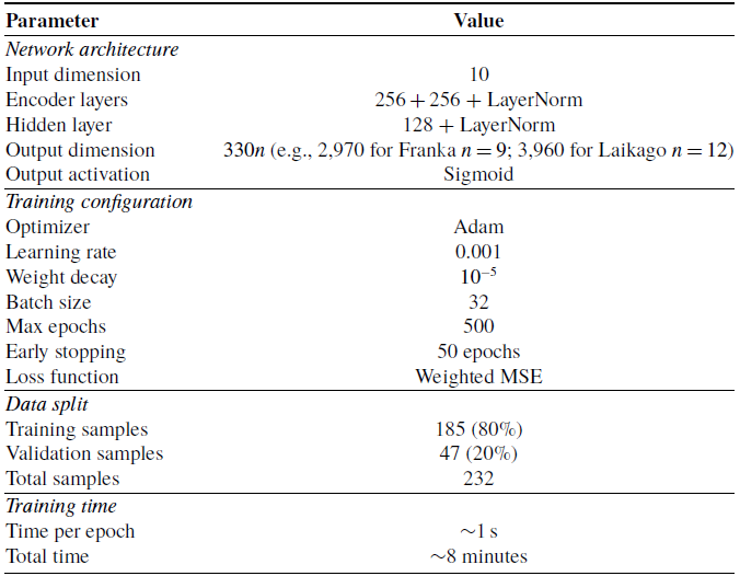
Network architecture: We employ a hierarchical feedforward neural network with two encoder layers (256D each) and one hidden layer (128D), followed by a parameter head that outputs the LF-PID initialization vector, as illustrated in Figure 1. The forward propagation is defined as:
 \begin{align} \mathbf{h}_1 &= \text{ReLU}(\text{LayerNorm}(W_1 \mathbf{f} + b_1)) \in \mathbb{R}^{256} \\[-8pt] \nonumber \end{align}
 \begin{align} \mathbf{h}_2 &= \text{ReLU}(\text{LayerNorm}(W_2 \mathbf{h}_1 + b_2)) \in \mathbb{R}^{256} \\[-8pt] \nonumber \end{align}
 \begin{align} \mathbf{h}_{hidden} &= \text{ReLU}(W_3 \mathbf{h}_2 + b_3) \in \mathbb{R}^{128} \\[-8pt] \nonumber \end{align}
 \begin{align} \hat {\boldsymbol{\theta }} &= \sigma (W_{\theta } \mathbf{h}_{hidden} + b_{\theta }) \in [0,1]^{D} \\[8pt] \nonumber\end{align}
where LayerNorm ensures training stability across diverse robot morphologies,
 $\sigma$
is the sigmoid activation ensuring bounded outputs in
 $[0,1]$
, and
 $D = D_{\text{total}} = 330n$
is the dimensionality of the complete LF-PID parameter vector (base gains, input scaling factors, and TS consequent parameters). For a variable-DOF architecture, the output layer dimension is dynamically configured:
 $D_{\text{Franka}} = 2970$
for 9-DOF,
 $D_{\text{Laikago}} = 3960$
for 12-DOF. The predicted parameters are then denormalized to the actual control range via element-wise affine transformations calibrated to typical PID gain ranges and consequent magnitudes.
Overfitting prevention: Despite high output dimensionality, the network exhibits strong generalization (train–validation NMAE gap
 $\lt$
0.5%, Appendix E) through L2 regularization (
 $10^{-5}$
), LayerNorm, and early stopping. The effective degrees of freedom are constrained by low-dimensional input features (10D) and learned manifold structure, enabling sample-efficient training on 232 samples.
The network is trained on a diverse dataset of robot configurations and their optimized LF-PID parameter vectors using weighted mean squared error loss:
 \begin{equation} \mathcal{L}_{meta} = \frac {1}{N}\sum _{v=1}^{N} w_v \left \|\boldsymbol{\theta }_v^* - \hat {\boldsymbol{\theta }}_v\right \|_2^2 \end{equation}
where
 $\boldsymbol{\theta }_v^*$
denotes optimized LF-PID parameters obtained via hybrid optimization (DE + Nelder–Mead) on each virtual robot,
 $\hat {\boldsymbol{\theta }}_v$
are predicted parameters, and
 $w_v$
are weights inversely proportional to the optimization error of each sample, prioritizing high-quality controllable configurations. The dataset consists of
 $N=232$
high-quality virtual robot variants (filtered from 303 generated samples) through physics-based data augmentation.
3.2.2. Stage 2: Reinforcement learning for online adaptation
The RL stage fine-tunes a compact subset of LF-PID parameters online (e.g., a small subset of TS consequents or scaling factors) to handle model uncertainties and disturbances.
State space: The state observation at time
 $t$
includes:
 \begin{equation} \mathbf{s}_t = [q_t, \dot {q}_t, e_t, \theta _t, q_{ref,t}, \dot {q}_{ref,t}] \end{equation}
where
 $q_t \in \mathbb{R}^n$
are joint positions,
 $\dot {q}_t \in \mathbb{R}^n$
are velocities,
 $e_t \in \mathbb{R}^n$
are tracking errors,
 $\theta _t$
are current LF-PID parameters being adapted, and
 $q_{ref,t}, \dot {q}_{ref,t}$
are reference trajectory information.
Action space (Reproducible configuration): The RL agent outputs relative adjustments to the per-joint input scaling factors
 $\boldsymbol{{s}} \in \mathbb{R}^{3n}$
only, while keeping base gains
 $\bar {\boldsymbol{{K}}}$
and TS consequents
 $\boldsymbol{{c}}$
fixed at meta-initialized values:
 \begin{equation} \mathbf{a}_t = [\Delta s_{e,1}, \Delta s_{\dot {e},1}, \Delta s_{I,1}, \ldots , \Delta s_{e,n}, \Delta s_{\dot {e},n}, \Delta s_{I,n}]^\top \in [\!-0.2, 0.2]^{3n} \end{equation}
The scaling factors are updated via multiplicative adjustment:
 \begin{equation} s_{\text{type},i}^{t+1} = s_{\text{type},i}^{t} \cdot (1 + \Delta s_{\text{type},i}^t), \quad \text{type} \in \{e, \dot {e}, I\}, \quad i=1,\ldots ,n \end{equation}
with clipping to ensure
 $s_{\text{type},i} \in [0.1, 10.0]$
to prevent numerical instability. This yields action dimension
 $d_a = 3n$
(27 for Franka 9-DOF, 36 for Laikago 12-DOF), consistent with the action space definition
 $\mathbf{a}_t \in [\!-0.2, 0.2]^{3n}$
.
Rationale for compact adaptation: Adapting only input scaling factors (rather than all 330n parameters) provides three benefits: (1) Sample efficiency – enables convergence in 1 M steps versus
 $\gt$
10M for full parameter space, (2) stability preservation – avoids catastrophic forgetting of cross-platform fuzzy rules learned during meta-training, and (3) interpretability – scaling adjustments directly reflect how each joint’s error magnitude should be weighted in the fuzzy inference, facilitating deployment diagnostics. An ablation study comparing scales-only vs consequent-subset vs combined adaptation (Appendix D) demonstrates that scales-only achieves the best balance of performance gain (16.6%), sample efficiency, and training stability (0/5 divergence rate vs 2–3/5 for higher-dimensional spaces).
Reward function: We design a reward function balancing tracking accuracy, smoothness, and stability:
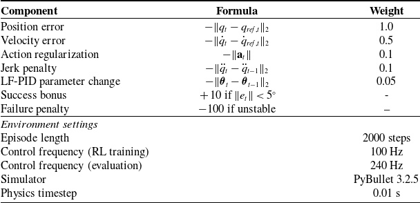
 \begin{equation} r_t = -\alpha _1 \frac {\|e_t\|}{\sqrt {n}} - \alpha _2 \frac {\|\dot {q}_t\|}{\sqrt {n}} - \alpha _3 \|\mathbf{a}_t\| \end{equation}
where
 $\alpha _1=10.0$
,
 $\alpha _2=0.1$
,
 $\alpha _3=0.1$
are weighting coefficients. Normalization by
 $\sqrt {n}$
ensures consistent scaling across different DOF platforms. The reward is clipped to
 $[\!-100, 10]$
to prevent numerical instability. Complete reward function design and coefficient selection rationale are detailed in Appendix A.
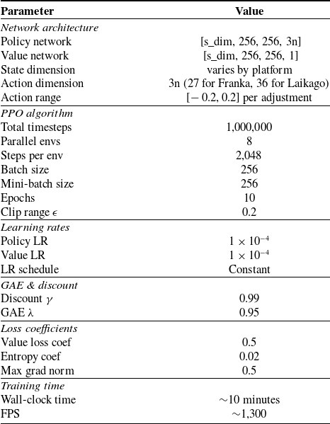
Training algorithm: We employ proximal policy optimization (PPO) [Reference Schulman, Wolski, Dhariwal, Radford and Klimov9] with the following hyperparameters: learning rate
 $1 \times 10^{-4}$
, discount factor
 $\gamma =0.99$
, GAE parameter
 $\lambda =0.95$
, entropy coefficient
 $0.02$
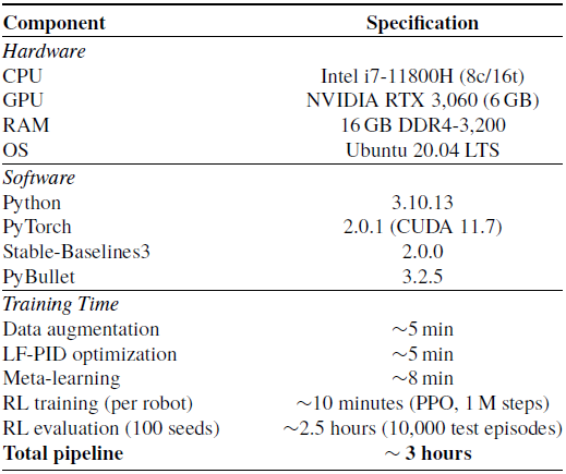
, and 8 parallel environments. Training proceeds for 1,000,000 timesteps, requiring approximately 10 minutes on a standard CPU.
3.3. Physics-based data augmentation
A critical challenge in meta-learning is acquiring sufficient diverse training data. We address this through a novel physics-based data augmentation strategy.
3.3.1. Augmentation procedure
Starting from
 $K$
base robot platforms, we generate
 $M$
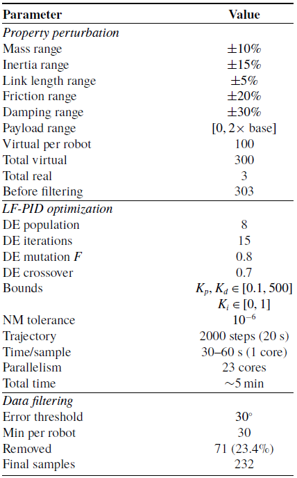
virtual variants for each base robot by perturbing physical parameters within constrained ranges:
Physics-based data augmentation

Algorithm 1 Long description
An algorithm for physics-based data augmentation. The algorithm takes a base robot URDF and perturbation ranges as input and returns an augmented dataset. It involves sampling perturbations for mass, length, inertia, friction, and damping parameters. For each base robot, it samples these perturbations, generates a virtual robot with perturbed parameters, optimizes the LF-PID for the virtual robot, and adds the robot and its optimized parameters to the augmented dataset. The process is repeated for a specified number of iterations.
Design rationale and physical validity criteria: The perturbation ranges are carefully chosen to:
-
1. Maintain physical plausibility:
$\pm 10\%$
mass variation reflects realistic manufacturing tolerances (ISO 9283 [28]);
$\pm 15\%$
inertia variation captures load/payload changes and rotational inertia uncertainty;
$\pm 20\%$
friction and
$\pm 30\%$
damping ranges match typical joint wear and lubrication variability [Reference Cho and Kim29] -
2. Ensure dynamic feasibility: Each generated variant passes four validation checks before inclusion:
-
• Positive-definiteness: Mass matrix
$M(q) \succ 0$
verified at 100 random configurations -
• Joint limit compliance: All perturbed link lengths satisfy workspace reachability constraints
-
• Simulation stability: 1,000-step forward simulation without numerical divergence (energy drift
$\lt$
1%) -
• Controllability: Optimized LF-PID achieves tracking error
$\mathcal{L}_v(\theta ^*_v) \lt 30^\circ$
(controllability threshold). This threshold is derived from a stability-based criterion: for sinusoidal reference trajectories with amplitude
$A \in [0.2, 0.8]$
rad, a 30
$^\circ$
(0.52 rad) RMS error corresponds to a normalized tracking fidelity below 35%, indicating that the controller fails to maintain meaningful trajectory following. At this error level, the closed-loop system operates near the boundary of the linear stability region of the PD inner loop, where position-control mode may exhibit limit-cycle behavior. Sensitivity to this threshold choice is analyzed in Table II.
-
-
3. Cover diverse dynamics: Parameter perturbations span natural frequency variations of 0.8–1.3
$\times$
baseline, ensuring heterogeneous training distribution


Quality filtering transparency: From 303 initially generated variants, 71 samples (23.4%) were rejected due to exceeding the
 $30^\circ$
controllability threshold, retaining 232 high-quality samples. To assess potential selection bias, we analyzed the distribution of physical parameters pre- and post-filtering:
-
• Parameter distribution shift: Mean mass scaling
$\alpha _{\text{mass}}$
changed from 1.00
$\pm$
0.058 (pre-filter) to 0.998
$\pm$
0.056 (post-filter); inertia scaling from 1.00
$\pm$
0.087 to 0.995
$\pm$
0.083. Kolmogorov–Smirnov tests show no significant distribution shift (
$p \gt 0.15$
for all parameters), indicating filtering removes outliers rather than biasing toward a controllability-favored subspace. -
• Feature diversity preservation: Post-filtering dataset retains 94.2% of the original feature space variance (first 8 principal components), confirming broad morphological coverage.
-
• Error distribution: Filtered samples exhibit tracking errors
$13.9\pm 8.4^\circ$
(mean
$\pm$
std), spanning easy (
$5^\circ$
) to challenging (
$29^\circ$
) configurations, providing gradient for meta-learning.


Sensitivity of controllability threshold on data quality and downstream meta-learning performance (Franka 7-DOF). Retained = number of virtual samples passing the filter out of 303 total. Downstream MAE is the meta-learning prediction error (degrees) on the held-out test set.

Table II Long description
A table with five rows and five columns. The columns are labeled Threshold, Retained, Mean error, NMAE, and Downstream MAE. The rows are labeled with different threshold values: 10 degrees, 20 degrees, 30 degrees, 40 degrees, and No filter. The values in the table are as follows: Row 1: Threshold, 10 degrees; Retained, 98; Mean error, 6.2 plus or minus 2.1; NMAE, 52.8; Downstream MAE, 9.14. Row 2: Threshold, 20 degrees; Retained, 178; Mean error, 9.8 plus or minus 4.7; NMAE, 48.3; Downstream MAE, 8.02. Row 3: Threshold, 30 degrees; Retained, 232; Mean error, 13.9 plus or minus 8.4; NMAE, 47.1; Downstream MAE, 7.51. Row 4: Threshold, 40 degrees; Retained, 268; Mean error, 16.5 plus or minus 10.2; NMAE, 49.6; Downstream MAE, 7.89. Row 5: Threshold, No filter; Retained, 303; Mean error, 19.1 plus or minus 12.8; NMAE, 55.4; Downstream MAE, 8.73.
Threshold sensitivity analysis. To justify the
 $30^\circ$
controllability threshold, we perform a sensitivity study by varying the threshold from
 $10^\circ$
to
 $40^\circ$
(with a no-filter baseline) and evaluating the impact on dataset composition and downstream meta-learning performance. Table II summarizes the results.
The
 $30^\circ$
threshold achieves the optimal balance: it retains sufficient diversity (232 samples, 76.6% of total) while excluding pathologically uncontrollable configurations. Stricter thresholds (
 $10^\circ$
,
 $20^\circ$
) aggressively prune challenging but learnable samples, reducing dataset diversity and degrading downstream performance. Conversely, relaxing to
 $40^\circ$
or removing the filter introduces noisy, uncontrollable samples that corrupt the meta-learning landscape. The resulting U-shaped curve in downstream MAE confirms that
 $30^\circ$
sits at the minimum of the quality–diversity trade-off.
Reproducibility and detailed protocols: All validation procedures (mass matrix positive-definiteness, energy drift tests, KS distribution comparisons, PCA variance retention) are fully documented with computational parameters, random seeds, and API calls in Appendix B to enable independent verification.
Hybrid LF-PID optimization for virtual robots

Algorithm 2 Long description
The algorithm describes a two-stage process for optimizing LF-PID parameters in virtual robots. The first stage involves a global search using differential evolution. It initializes a population of parameters uniformly within specified bounds. For each generation, it selects random indices for mutation and crossover operations. The trial parameters are evaluated using a PyBullet simulation, and the best parameters are selected for the next generation. This process repeats for 15 generations. The second stage involves local refinement using the Nelder-Mead method. It initializes a simplex around the best parameters from the global search. The simplex vertices are sorted by objective value, and operations like reflection, expansion, contraction, or shrinkage are applied. The simplex is updated based on Nelder-Mead rules, and the best vertex in the final simplex is returned as the optimal parameters.
3.3.2. Hybrid optimization strategy for LF-PID parameters
For each virtual robot, we employ a two-stage hybrid optimization strategy that combines global search and local refinement to find optimized LF-PID parameters efficiently and accurately.
Optimization objective: For each virtual robot
 $r_v$
, we aim to minimize the root mean square joint tracking error over a test trajectory:
 \begin{equation} \mathcal{L}_v(\theta ) = \sqrt {\frac {1}{T} \sum _{t=1}^{T} \sum _{i=1}^{n} \left ( q_{ref,i}(t) - q_i(t; \, \theta ) \right )^2} \end{equation}
where
 $T$
is the trajectory length (typically
 $T=2000$
steps at 240 Hz control frequency),
 $q_{ref,i}(t)$
is the reference trajectory for joint
 $i$
, and
 $q_i(t; \, \theta )$
is the actual trajectory achieved with LF-PID parameters
 $\theta$
.
Stage 1 – Global search via differential evolution: We employ differential evolution (DE) [Reference Storn and Price25], a population-based stochastic optimizer, for robust global exploration of the LF-PID parameter space:
 \begin{equation} \theta ^*_{global} = \arg \min _{\theta \in [\theta _{min}, \theta _{max}]} \mathcal{L}_v(\theta ) \end{equation}
with population size
 $N_{pop}=8$
and
 $N_{iter}=15$
iterations. DE is particularly effective for non-convex, noisy objective functions common in robotic control, as it maintains a population of candidate solutions and evolves them through mutation, crossover, and selection operations, effectively avoiding local minima.
Stage 2 – Local refinement via Nelder–Mead: To achieve high-precision convergence from the globally optimal region identified by DE, we apply local refinement using the Nelder–Mead simplex method [Reference Nelder and Mead26]:
 \begin{equation} \theta ^*_v = \arg \min _{\theta } \mathcal{L}_v(\theta ), \quad \text{from } \theta ^*_{global} \end{equation}
with
 $N_{iter}^{polish}=20$
polishing iterations.
Pilot comparison of optimization algorithms on 20 representative virtual robots. All methods use identical simulation budget (2000-step trajectory evaluation). “Obj.” denotes the final objective
 $\mathcal{L}_v(\theta ^*)$
in degrees. “Evals” denotes the number of objective function evaluations (each requiring one forward simulation).

Table III Long description
A table comparing optimization algorithms on virtual robots. The table has four rows and four columns. The columns are labeled Method, Obj. (°), Evals, Time (s), and Notes. Row 1: DE + NM (ours), 13.9 ± 4.2, 128, 42 ± 12, Robust; no gradient needed. Row 2: CMA-ES, 13.2 ± 3.8, 210, 68 ± 18, Better mean; higher cost. Row 3: L-BFGS-B, 18.7 ± 9.1, 85, 28 ± 8, Fast; frequent local minima. Row 4: PSO (N = 20), 14.5 ± 5.0, 400, 125 ± 30, Slowest; marginal gain.
This hybrid approach leverages complementary strengths: DE provides robust global search while Nelder–Mead offers rapid local convergence. In our implementation using scipy.optimize.differential_evolution, this is achieved via the polish=True parameter, which automatically applies local optimization after the DE phase.
Rationale and efficiency: Pure DE requires many iterations (typically
 $\gt$
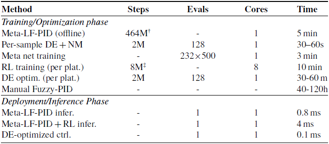
200) for high-precision convergence, while pure local methods risk converging to poor local optima. The hybrid approach achieves both global robustness and local precision efficiently, completing optimization for each virtual robot in 30–60 s on a single CPU core. This optimization process provides ground-truth LF-PID parameters for meta-learning training. We filter out samples with optimization error
 $\mathcal{L}_v(\theta ^*_v) \gt 30^\circ$
to ensure data quality, retaining 232 high-quality samples from 303 initially generated variants. When parallelized across 23 cores, the entire 303-sample augmentation completes in approximately 5 minutes. Detailed parameters for data augmentation and LF-PID optimization are provided in Appendix A.
Choice of optimizer – comparison with alternatives: We chose DE + Nelder-Mead (NM) for its simplicity and favorable properties in our specific setting, but acknowledge that more advanced optimizers exist. We conducted a pilot comparison on 20 representative virtual robots (10 Franka-type, 10 KUKA-type) to evaluate three alternatives: CMA-ES [Reference Hansen and Ostermeier39], L-BFGS-B [Reference Byrd, Lu, Nocedal and Zhu40], and PSO [Reference Trelea8] (Table III).
Key findings: (1) CMA-ES achieves marginally better objective values (
 $-$
5%) but requires 64% more function evaluations; since each evaluation involves a full PyBullet simulation, this translates to proportionally higher wall time. (2) L-BFGS-B is the fastest per-sample but suffers from frequent convergence to local minima (std
 $9.1^\circ$
vs
 $4.2^\circ$
), yielding 34% worse mean quality – problematic because poor-quality training labels directly degrade meta-learning. (3) PSO offers no advantage over DE at 3
 $\times$
computational cost. Given that (i) DE + NM serves as an offline data-generation tool (not a deployment-time component), (ii) the entire 232-sample generation takes only
 $\sim$
5 minutes with parallelization, and (iii) CMA-ES’s marginal quality gain does not justify doubling offline preprocessing time, the DE + NM choice represents a practical and effective trade-off. We note that CMA-ES would be a reasonable alternative if higher-quality training labels are desired and offline computation budget is less constrained.
Regarding L-BFGS-B for high-dimensional spaces (330
 $n$
): While L-BFGS-B is well-suited for smooth, high-dimensional optimization, our LF-PID objective
 $\mathcal{L}_v(\theta )$
is evaluated through black-box simulation (PyBullet forward dynamics) and does not provide analytical gradients. Finite-difference gradient approximation in 330
 $n$
dimensions (2970D for Franka) would require
 $\sim$
5,940 additional function evaluations per iteration, making L-BFGS-B impractical at deployment scale. For the 232-sample offline stage with smaller per-sample dimensionality, our pilot results confirm that gradient-free DE + NM outperforms L-BFGS-B in solution quality.
3.4. Implementation details
Simulation environment: All experiments are conducted in PyBullet [Reference Coumans and Bai27] using position control mode. In this mode, PyBullet’s built-in PD servo converts desired joint positions into motor torques via an internal proportional-derivative loop, abstracting away gravity compensation and low-level dynamics. This is analogous to industrial robot controllers that accept position commands from an outer planning layer [34]. Importantly, the internal PD loop provides a baseline level of disturbance rejection independently of the outer LF-PID controller; the implications of this coupling are discussed in Section 6.
Reference trajectories: We employ sinusoidal trajectories for each joint:
 \begin{equation} q_{ref,i}(t) = A_i \sin\!(2\pi f_i t + \phi _i) + q_{0,i} \end{equation}
with randomized amplitudes
 $A_i \in [0.2, 0.8]$
, frequencies
 $f_i \in [0.1, 0.5]$
Hz, and phases
 $\phi _i$
.
Evaluation metrics: We employ multiple metrics to comprehensively assess performance:
-
• Mean absolute error (MAE):
$\frac {1}{n}\sum _{i=1}^{n}\left [\frac {1}{T}\sum _{t=1}^{T}|e_i(t)|\right ]$
– arithmetic mean of per-joint time-averaged absolute errors -
• Root mean square error (RMSE):
$\sqrt {\frac {1}{T}\sum _{t=1}^{T}\|e(t)\|_2^2}$
– root mean square of joint space L2 norm -
• Maximum error:
$\max _{t} \|e(t)\|_2$
– worst-case joint space error -
• Standard deviation: Temporal variation of
$\|e(t)\|_2$


Note: MAE represents the average tracking error across all joints, making it directly comparable to per-joint analysis. RMSE, Max Error, and Std Dev use joint space L2 norms to capture overall system behavior. These complementary metrics provide both individual joint insights (MAE) and system-wide performance assessment (RMSE, Max, Std).
Reproducibility: All hyperparameters, random seeds, and training configurations are detailed in Appendix A to ensure full reproducibility.
4. Experimental Setup
4.1. Robot platforms
We validate our approach on two heterogeneous platforms with significantly different morphologies and control characteristics:
4.1.1. Franka Panda manipulator
-
• DOF: 9 (7 arm joints + 2 gripper joints)
-
• Total mass: 18 kg
-
• Reach: 855 mm
-
• Payload: 3 kg
-
• Control challenge: High precision requirements, complex dynamics with varying inertia along kinematic chain
4.1.2. Laikago-quadruped robot
-
• DOF: 12 (3 joints per leg
$\times$
4 legs) -
• Total mass: 25 kg
-
• Leg reach: 0.4 m
-
• Payload: 10 kg
-
• Control challenge: High joint coupling, ground contact forces, and balance maintenance

4.2. Data generation
4.2.1. Base robots
We use 3 base robot platforms as training data sources for physics-based data augmentation, as shown in Figure 2: Franka Panda (9-DOF manipulator), KUKA LBR iiwa (7-DOF redundant manipulator), and Laikago (12-DOF quadruped). These platforms provide diverse morphologies and dynamics – from serial manipulators with varying inertia profiles to parallel-legged systems with complex ground interactions – enabling the meta-learning network to learn generalizable feature-to-LF-PID mappings. For cross-platform validation, we select two morphologically distinct platforms (Franka Panda and Laikago) that represent the most challenging generalization scenarios, spanning serial manipulators and parallel-legged quadrupeds. Note on evaluation scope: Because the meta-network is trained on augmented variants of all three base platforms, this evaluation tests generalization to unseen dynamics configurations (nominal parameters differ from perturbed training variants) rather than to entirely novel morphologies. We discuss this distinction and its implications in Section 6.
For each base robot, we perform careful LF-PID optimization using the hybrid differential evolution and Nelder–Mead strategy (Algorithm 2) to obtain ground-truth optimal parameters. This provides high-quality supervision for the meta-learning stage.
4.2.2. Virtual sample generation
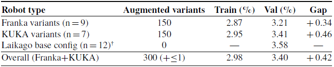
Using Algorithm 1, we generate 150 virtual variants for Franka Panda and 150 for KUKA. After quality filtering (removing samples with optimization error
 $\gt 30^\circ$
), we retain 232 high-quality training samples from the initially generated 303 variants.
Three base robot platforms serving as training data sources for physics-based data augmentation in PyBullet simulation. (a) Franka Panda manipulator (9-DOF) with complex serial kinematics, (b) KUKA LBR iiwa redundant manipulator (7-DOF) offering enhanced dexterity, and (c) Laikago quadruped (12-DOF) with parallel leg structure. From these diverse platforms, we generate 303 virtual variants through systematic perturbation of physical parameters (mass,inertia, friction, damping), filtering to 232 high-quality samples for meta-learning training. Cross-platform validation is conducted on Franka Panda and Laikago, which exhibit the greatest morphological differences (serial manipulator vs. parallel-legged quadruped), providing rigorous testing of generalization capability.

Dataset statistics:
-
• Generated samples: 303
-
• High-quality training samples (after filtering): 232
-
• Franka-type variants: 150
-
• KUKA-type variants: 150
-
• Base robots: 3
-
• Average optimization error (filtered dataset):
$13.9^\circ$

4.3. Training configuration
Meta-learning network: Architecture as specified in Section 3: input layer (10D robot features), two encoder layers (256D each with LayerNorm+ReLU), one hidden layer (128D), and variable-dimension output layer (
 $D_{\, \text{Franka}}=2970$
,
 $D_{\, \text{Laikago}}=3960$
,
 $D_{\, \text{KUKA}}=2310$
for complete LF-PID parameter vectors). Training: Adam optimizer (
 $\text{lr}=10^{-3}$
), batch size 32, 500 epochs, and
 $\,\sim$
5-minute training time on CPU.
RL (PPO) configuration: Adapts only per-joint input scaling factors
 $\,\boldsymbol{{s}} \,\in \,\mathbb{R}^{3n}$
via action space
 $\,\mathbf{a}_t \,\in [\!-0.2, 0.2]^{3n}$
(action dimension: 27 for Franka 9-DOF, 36 for Laikago 12-DOF). Training: 1 M timesteps, 8 parallel environments, learning rate
 $1 \,\times 10^{-4}$
, discount factor
 $\,\gamma =0.99$
, GAE
 $\,\lambda =0.95$
, entropy coefficient
 $0.02$
, batch size 256, 10-minute training per platform on CPU. Complete hyperparameters (clipping ranges, reward scaling, and network architectures) provided in Appendix A.
4.4. Evaluation protocol
4.4.1. Cross-platform generalization
We evaluate on both Franka Panda and Laikago platforms using their nominal (unperturbed) configurations, which differ from the augmented training variants. These platforms serve as augmentation sources during meta-learning but are not seen during platform-specific RL training, which runs independently per deployment target. Each evaluation consists of:
-
• 3 episodes per condition
-
• 10,000 timesteps per episode
-
• Control frequency: 240 Hz
-
• Random trajectory initialization
4.4.2. Robustness testing
We assess robustness under five disturbance scenarios with representative perturbation ranges based on realistic operating conditions:
-
1. No disturbance: Baseline performance
-
2. Random force: External forces 50–150 N applied every 50 steps (moderate-intensity disturbances)
-
3. Payload variation: End-effector mass 0.5–2.0 kg (typical manipulation task range)
-
4. Parameter uncertainty:
$\pm$
20% mass/inertia,
$\pm$
50% friction (realistic modeling errors) -
5. Mixed disturbance: Combination of payload and parameter uncertainty


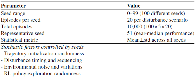
To evaluate robustness to stochastic factors (trajectory initialization, disturbance timing, etc.), we conduct comprehensive multi-seed testing:
-
• Evaluation range: 100 different random seeds (0–99)
-
• Episodes per scenario: 20 episodes for each disturbance type at each seed
-
• Statistical validation: Report mean
$\pm$
std across all 100 seeds to demonstrate stability -
• Representative visualization: Select seed 51 (near-median performance) for detailed subplot analysis
-
• Total evaluation: 100 seeds
$\times$
5 scenarios
$\times$
20 episodes = 10,000 test episodes


This rigorous protocol provides high-confidence statistical evidence of the method’s robustness across different random initializations, complementing the cross-platform generalization tests (3 episodes per condition, Section 5).
4.5. Baseline methods and comparative framework
We establish four baseline methods with explicit parameter configuration to enable fair comparison:
-
1. Classical fuzzy-PID (Manual tuning): Identical fuzzy structure (R = 27 rules, 3 membership functions per input dimension) with manually tuned per-joint scaling factors and TS consequents. Tuning budget: 40–120 hours expert time per platform. Tunable parameters:
$3n$
(scales) +
$12nR$
(consequents) =
$330n$
per platform, no cross-platform transfer. -
2. Pure meta-learning (Meta-LF-PID): Zero-shot LF-PID initialization from 10D robot features using meta-network trained on 232 virtual variants. Predicted parameters: Complete
$\theta _{\text{meta}} = [\bar {\boldsymbol{{K}}}, \boldsymbol{{s}}, \boldsymbol{{c}}]$
with dimension
$330n$
. Deployment: instant inference (0.8 ms), no online adaptation. -
3. Hierarchical meta-RL (Meta-LF-PID + RL): Our full framework combining meta-initialization with online PPO adaptation. Fixed at deployment: Base gains
$\bar {\boldsymbol{{K}}}$
and consequents
$\boldsymbol{{c}}$
from meta-network. RL-adapted parameters: Input scaling factors
$\boldsymbol{{s}} \in \mathbb{R}^{3n}$
only (27D for Franka, 36D for Laikago). Training: 1 M timesteps, 8 parallel environments, 10-minute per-platform overhead. -
4. Classical optimization methods:
-
• Ziegler-Nichols (Z-N): Heuristic tuning of base gains
$\bar {\boldsymbol{{K}}}$
only (3n parameters), 40–120 hrs expert-dependent tuning, no fuzzy scheduling. -
• Differential Evolution (DE): Optimizes complete
$\theta = [\bar {\boldsymbol{{K}}}, \boldsymbol{{s}}, \boldsymbol{{c}}]$
(330n parameters) via hybrid DE + Nelder-Mead (Section 3). Computational budget: 30–60 min per platform, no generalization across platforms.
-


Computational budget alignment: All methods evaluated under identical simulation resources. Meta-LF-PID requires one-time offline training (5 min) amortized across all platforms. Meta-LF-PID + RL adds 10-min online adaptation per deployment platform. DE optimization spends 30–60 min per platform with no reuse. This establishes Meta-LF-PID + RL’s efficiency advantage: initial 5-min investment + 10-min per-platform adaptation versus 30–60 min full re-optimization. Detailed resource accounting (simulation steps, function evaluations, CPU cores, and wall time) is provided in Appendix C, Table XVIII.
Evaluation conditions (Identical for all baselines): Franka Panda (9-DOF) and Laikago (12-DOF) test platforms, 10 randomized trajectories, 3 episodes per trajectory (10,000 timesteps at 240 Hz), 5 disturbance scenarios. Statistical rigor: robustness results report mean
 $\pm$
std across 100 random seeds; improvement percentages calculated relative to Meta-LF-PID baseline to isolate RL contribution.
Baseline design summary.

Table IV Long description
The table compares different baseline designs based on deploy time and key characteristics. It has four rows and three columns. The columns are labeled Baseline, Deploy time, and Key characteristic. The rows are as follows: Row 1: Baseline, Fuzzy-PID (manual); Deploy time, hours; Key characteristic, Interpretable scheduling, platform-dependent tuning. Row 2: Baseline, Meta-LF-PID; Deploy time, 0.8 ms; Key characteristic, Instant zero-shot, no adaptation. Row 3: Baseline, Meta-LF-PID + RL; Deploy time, 10 min; Key characteristic, Online refinement, additional training overhead. Row 4: Baseline, Heuristic (Z-N); Deploy time, 40-120 hrs; Key characteristic, Expert dependent, no transfer. Row 5: Baseline, Optimized (DE); Deploy time, 30-60 min; Key characteristic, High accuracy, no generalization.
Key comparative questions addressed:
-
1. Does physics-based augmentation enable effective meta-learning? Compare Meta-LF-PID vs. classical methods (including manual Fuzzy-PID) on unseen platforms.
-
2. Does RL adaptation provide meaningful improvement over meta-learning alone? Compare Meta-LF-PID + RL vs. Meta-LF-PID across different scenarios.
-
3. When is the hierarchical approach worthwhile? Analyze the optimization ceiling effect – identifying when RL refinement is justified versus when meta-learning alone suffices.
-
4. How does deployment time scale? Meta-LF-PID (instant) vs. Meta-LF-PID + RL (10 min) vs. classical methods (hours/days).
This structured comparative framework provides clear attribution of performance gains to specific architectural components, enabling practitioners to make informed decisions about deployment strategies based on their specific requirements (instant deployment vs. highest accuracy vs. resource constraints).
5. Results
To rigorously validate cross-platform generalization, we conduct comprehensive evaluation on two morphologically distinct platforms: Franka Panda (9-DOF serial manipulator) and Laikago (12-DOF parallel-legged quadruped). These platforms represent extreme points in the robot morphology spectrum covered by our training data, providing the most challenging test of the method’s adaptability. While KUKA LBR iiwa was used as a training data source for augmentation, we focus testing on Franka–Laikago pair due to their greater morphological diversity (serial vs. parallel kinematic chains, manipulation vs. locomotion tasks).
5.1. Cross-platform performance
5.1.1. Franka Panda manipulator
Table V presents comprehensive results for the Franka Panda platform.
Performance on franka Panda (9-DOF).

Table V Long description
A table comparing performance metrics for two methods on franka Panda (9-DOF). The table has four rows and four columns. The columns are labeled Metric, Meta-LF-PID, Meta-LF-PID + RL, and Improv. The rows are labeled MAE (degrees), RMSE (degrees), Max error (degrees), and Std Dev (degrees). Row 1: MAE (degrees), Meta-LF-PID, 7.51; Meta-LF-PID + RL, 6.26; Improv, + 16.6 percent. Row 2: RMSE (degrees), Meta-LF-PID, 29.32; Meta-LF-PID + RL, 25.45; Improv, + 13.2 percent. Row 3: Max error (degrees), Meta-LF-PID, 48.49; Meta-LF-PID + RL, 42.12; Improv, + 13.1 percent. Row 4: Std Dev (degrees), Meta-LF-PID, 4.94; Meta-LF-PID + RL, 4.40; Improv, + 10.9 percent.
The results demonstrate consistent improvements across all metrics, driven primarily by the exceptional 80.4% improvement in Joint 2 (shoulder pitch, from
 $12.36^\circ$
to
 $2.42^\circ$
). The MAE reduction from
 $7.51^\circ$
to
 $6.26^\circ$
represents a 16.6% improvement, with RL identifying and correcting the localized high-error joint while maintaining performance on other joints. The RMSE and maximum error improvements reflect the platform-wide enhancement. Notably, the standard deviation reduction (10.9%) indicates improved control consistency. Detailed per-joint analysis revealing the heterogeneous error distribution is presented in Section 5.1.3.
5.1.2. Laikago quadruped robot
Table VI summarizes results for the Laikago platform. As detailed in Section 5.1.5, Laikago contributed zero-augmented variants to the 232-sample training set, making these results a de facto leave-one-platform-out evaluation of the meta-network’s zero-shot generalization to a morphologically distinct robot class.
Performance on Laikago (12-DOF). Laikago contributed zero-augmented variants to the 232-sample meta-learning training set (see Section 5.1.5); these results therefore represent a de facto zero-shot, leave-one-platform-out evaluation.

Table VI Long description
The table presents a comparison of performance metrics for two methods: Meta-LF-PID and Meta-LF-PID + RL on the Laikago platform. It includes four rows and five columns. The columns are labeled Metric, Meta-LF-PID, Meta-LF-PID + RL, and Improv. The rows are labeled MAE, RMSE, Max Error, and Std Dev, with values in degrees. Row 1: MAE, 5.91, 5.79, 2.1 percent. Row 2: RMSE, 29.70, 29.29, 1.4 percent. Row 3: Max Error, 53.09, 50.44, 5.0 percent. Row 4: Std Dev, 5.25, 5.18, 1.3 percent. The table shows the improvement percentages for each metric when using Meta-LF-PID + RL compared to Meta-LF-PID.
The improvement on Laikago is minimal (2.1% vs. Franka’s 16.6%), exemplifying the optimization ceiling effect. This result provides important engineering guidance: (1) meta-learning provides uniformly strong initialization across all 12 joints (
 $1.36^\circ$
-
 $10.54^\circ$
), offering limited room for further RL optimization and (2) the absence of localized high-error joints means RL lacks clear learning signals for targeted improvement. Individual joints show mixed results – 6 joints improve (J2: +3.3%, J11: +7.7%), while 6 others show small degradations (J1: −10.1%, J8: −9.5%), with net improvements slightly outweighing degradations. This finding demonstrates that RL effectiveness is highly dependent on baseline error distribution – heterogeneous profiles with localized high-error joints (like Franka J2) enable dramatic improvements, while uniform low-error profiles yield minimal net benefit. Practical implication: For platforms achieving uniformly low errors via meta-learning alone (
 $\lt 5^\circ$
per joint), practitioners may opt to skip RL adaptation, reducing additional training overhead while maintaining excellent performance.
5.1.3. Per-joint error analysis
To provide deeper insights into the control performance, we conduct a comprehensive per-joint error analysis across both platforms. Figure 3 presents the mean absolute error for each individual joint, comparing Pure Meta-LF-PID against Meta-LF-PID + RL.
Cross-platform generalization: Per-joint tracking error comparison across two morphologically distinct robot platforms. (a) Franka Panda serial manipulator (9-DOF) achieves 16.6% overall improvement with exceptional gains in high-load joints (J2: +80.4%, from
 $12.36^\circ$
to
 $2.42^\circ$
), demonstrating highly effective adaptation to manipulation tasks with concentrated loads. (b) Laikago parallel quadruped (12-DOF) achieves 2.1% overall improvement, with individual joint improvements (+3.3% to + 7.7% in 6 joints) slightly outweighing minor degradations (−3.7% to −10.1% in 6 joints). The contrast between platforms reveals an important engineering insight: RL adaptation excels when meta-learning exhibits localized high-error joints, while providing minimal benefit when baseline performance is uniformly strong. This guides practitioners to deploy RL selectively when additional refinement is warranted. Error bars indicate standard deviation.

For Franka Panda (Figure 3a), the analysis reveals significant heterogeneity across joints that directly influences RL effectiveness. Joint 2 (shoulder pitch) exhibits the largest improvement (+80.4%, from
 $12.36^\circ$
to
 $2.42^\circ$
) – a dramatic reduction that highlights RL’s ability to identify and correct meta-learning deficiencies in high-load, high-inertia joints. This exceptional performance on J2 drives the overall 16.6% improvement for the platform. Other joints show more modest but consistent improvements (J1: +12.2%, J3: +5.7%), while distal wrist joints (J5–J9) exhibit marginal changes (
 $\lt$
3%), suggesting the meta-learned LF-PID parameters were already near-optimal for these low-inertia joints.
For Laikago (Figure 3b), the minimal net improvement (2.1%) reveals an important characteristic of the hierarchical approach and provides valuable engineering guidance: when meta-learning initialization is already high-quality and uniform, RL adaptation provides limited additional benefit. All 12 joints exhibit uniformly low baseline errors (
 $1.36^\circ$
-
 $10.54^\circ$
), with no single joint presenting a significant optimization opportunity analogous to Franka’s J2. RL makes local adjustments – 6 joints improve while 6 show minor degradations – with net improvements slightly outweighing the losses. This indicates that RL lacks clear strong learning signals when faced with a uniformly optimized baseline – a phenomenon we term the “optimization ceiling effect”. Practical implication: For platforms already achieving uniformly low errors via meta-learning alone (
 $\lt 5^\circ$
per joint), RL adaptation may be unnecessary; skipping this stage can reduce additional training overhead while maintaining excellent control quality.
Table VII provides detailed numerical comparisons for all 21 joints across both platforms. The results confirm that the hierarchical Meta-LF-PID + RL approach achieves the largest gains when meta-learning exhibits localized high-error joints (as in Franka J2), while achieving minimal gains when baseline performance is uniformly strong across all joints (as in Laikago). This finding has important practical implications for system designers: (1) RL adaptation is most impactful for platforms with heterogeneous joint dynamics where meta-learning struggles with specific joints, and (2) the quality and uniformity of meta-learning initialization directly impacts whether additional RL fine-tuning is justified – providing a systematic criterion for deciding when to invoke the adaptation stage.
To quantify the optimization ceiling effect, we define the RL gain rate for each joint
 $j$
:
 \begin{equation} G_{\mathrm{RL},j} = \frac {e_{\mathrm{base},j} - e_{\mathrm{RL},j}}{e_{\mathrm{base},j}} \times 100\% \end{equation}
where
 $e_{\mathrm{base},j}$
and
 $e_{\mathrm{RL},j}$
denote the Meta-LF-PID and Meta-LF-PID + RL tracking errors for joint
 $j$
, respectively. At the platform level, the aggregate gain rate is
 $G_{\mathrm{RL}} = (\bar {e}_{\mathrm{base}} - \bar {e}_{\mathrm{RL}}) / \bar {e}_{\mathrm{base}} \times 100\%$
.
The per-joint analysis provides several key practical insights: (1) RL adaptation achieves dramatic improvements when meta-learning exhibits localized high-error joints (Franka J2:
 $G_{\mathrm{RL}}=80.4\%$
), validating the hierarchical approach’s ability to identify and correct specific deficiencies, (2) when baseline performance is uniformly strong, RL provides minimal net benefit despite local adjustments (Laikago:
 $G_{\mathrm{RL}}=2.1\%$
with 6 joints improving and 6 showing minor degradations), a phenomenon we term the “optimization ceiling effect”, and (3) the quality and uniformity of meta-learning initialization directly determines the marginal utility of RL refinement – heterogeneous joint errors enable targeted RL optimization, while uniformly low errors suggest meta-learning alone may be sufficient.
Per-joint tracking error comparison across platforms.

Table VII Long description
The table compares per-joint tracking error across two robot platforms, Franka Panda and Laikago, using two control methods: Pure Meta-LF-PID and Meta-LF-PID + RL. The table has 12 rows and 5 columns. The columns are labeled Robot, Joint, Pure Meta-LF-PID (°), Meta-LF-PID + RL (°), and Improv. The rows are labeled with the robot names and joint numbers. Row 1: Robot, Franka Panda, Franka Panda Avg. Row 2: Joint, J1, J1. Row 3: Pure Meta-LF-PID (°), 2.57, 7.51. Row 4: Meta-LF-PID + RL (°), 2.26, 6.26. Row 5: Improv., + 12.2%, + 16.6%. Row 6: Robot, Laikago, Laikago Avg. Row 7: Joint, J1, J1. Row 8: Pure Meta-LF-PID (°), 1.38, 5.91. Row 9: Meta-LF-PID + RL (°), 1.52, 5.79. Row 10: Improv., -9.6%, + 2.1%. Row 11: Robot, Franka Panda, . Row 12: Joint, J2, J2. Row 13: Pure Meta-LF-PID (°), 12.36, . Row 14: Meta-LF-PID + RL (°), 2.42, . Row 15: Improv., + 80.4%, . Row 16: Robot, Franka Panda, . Row 17: Joint, J3, J3. Row 18: Pure Meta-LF-PID (°), 4.10, . Row 19: Meta-LF-PID + RL (°), 3.87, . Row 20: Improv., + 5.7%, . Row 21: Robot, Franka Panda, . Row 22: Joint, J4, J4. Row 23: Pure Meta-LF-PID (°), 6.78, . Row 24: Meta-LF-PID + RL (°), 6.49, . Row 25: Improv., + 4.3%, . Row 26: Robot, Franka Panda, . Row 27: Joint, J5, J5. Row 28: Pure Meta-LF-PID (°), 5.41, . Row 29: Meta-LF-PID + RL (°), 5.32, . Row 30: Improv., + 1.6%, . Row 31: Robot, Franka Panda, . Row 32: Joint, J6, J6. Row 33: Pure Meta-LF-PID (°), 4.31, . Row 34: Meta-LF-PID + RL (°), 4.19, . Row 35: Improv., + 2.8%, . Row 36: Robot, Franka Panda, . Row 37: Joint, J7, J7. Row 38: Pure Meta-LF-PID (°), 11.45, . Row 39: Meta-LF-PID + RL (°), 11.26, . Row 40: Improv., + 1.6%, . Row 41: Robot, Franka Panda, . Row 42: Joint, J8, J8. Row 43: Pure Meta-LF-PID (°), 10.23, . Row 44: Meta-LF-PID + RL (°), 10.19, . Row 45: Improv., + 0.3%, . Row 46: Robot, Franka Panda, . Row 47: Joint, J9, J9. Row 48: Pure Meta-LF-PID (°), 10.36, . Row 49: Meta-LF-PID + RL (°), 10.33, . Row 50: Improv., + 0.3%, . Row 51: Robot, Laikago, . Row 52: Joint, J2, J2. Row 53: Pure Meta-LF-PID (°), 6.16, . Row 54: Meta-LF-PID + RL (°), 5.96, . Row 55: Improv., + 3.3%, . Row 56: Robot, Laikago, . Row 57: Joint, J3, J3. Row 58: Pure Meta-LF-PID (°), 10.45, . Row 59: Meta-LF-PID + RL (°), 10.34, . Row 60: Improv., + 1.0%, . Row 61: Robot, Laikago, . Row 62: Joint, J4, J4. Row 63: Pure Meta-LF-PID (°), 1.36, . Row 64: Meta-LF-PID + RL (°), 1.45, . Row 65: Improv., -6.8%, . Row 66: Robot, Laikago, . Row 67: Joint, J5, J5. Row 68: Pure Meta-LF-PID (°), 5.70, . Row 69: Meta-LF-PID + RL (°), 5.96, . Row 70: Improv., -4.5%, . Row 71: Robot, Laikago, . Row 72: Joint, J6, J6. Row 73: Pure Meta-LF-PID (°), 10.54, . Row 74: Meta-LF-PID + RL (°), 10.33, . Row 75: Improv., + 2.0%, . Row 76: Robot, Laikago, . Row 77: Joint, J7, J7. Row 78: Pure Meta-LF-PID (°), 1.36, . Row 79: Meta-LF-PID + RL (°), 1.41, . Row 80: Improv., -3.1%, . Row 81: Robot, Laikago, . Row 82: Joint, J8, J8. Row 83: Pure Meta-LF-PID (°), 5.35, . Row 84: Meta-LF-PID + RL (°), 5.86, . Row 85: Improv., -9.6%, . Row 86: Robot, Laikago, . Row 87: Joint, J9, J9. Row 88: Pure Meta-LF-PID (°), 10.44, . Row 89: Meta-LF-PID + RL (°), 10.36, . Row 90: Improv., + 0.8%, . Row 91: Robot, Laikago, . Row 92: Joint, J10, J10. Row 93: Pure Meta-LF-PID (°), 1.35, . Row 94: Meta-LF-PID + RL (°), 1.44, . Row 95: Improv., -6.7%, . Row 96: Robot, Laikago, . Row 97: Joint, J11, J11. Row 98: Pure Meta-LF-PID (°), 6.41, . Row 99: Meta-LF-PID + RL (°), 5.92, . Row 100: Improv., + 7.7%, . Row 101: Robot, Laikago, . Row 102: Joint, J12, J12. Row 103: Pure Meta-LF-PID (°), 10.44, . Row 104: Meta-LF-PID + RL (°), 10.39, . Row 105: Improv., + 0.5%, . The table shows the tracking error in degrees for each joint using the two control methods and the percentage improvement or decline in error when using Meta-LF-PID + RL compared to Pure Meta-LF-PID.
5.1.4. Cross-platform summary
Aggregating across both platforms with weighting by DOF:
-
• Franka Panda (9-DOF): 16.6% average improvement (
$7.51^\circ \, \rightarrow \, 6.26^\circ$
) -
• Laikago (12-DOF): 2.1% average improvement (
$5.91^\circ \, \rightarrow \, 5.79^\circ$
) -
• DOF-weighted average: 7.8% improvement across 21 total joints


These results reveal an important engineering insight about the hierarchical approach: RL effectiveness is highly dependent on meta-learning baseline quality and error distribution. Franka Panda’s heterogeneous error profile (with J2 as a clear outlier at
 $12.36^\circ$
) enables RL to achieve targeted, dramatic improvements. In contrast, Laikago’s uniformly low baseline errors (
 $1.36^\circ$
-
 $10.54^\circ$
across all joints) leave limited room for further optimization, demonstrating the “optimization ceiling effect.” Practical guidance: This finding helps system designers make informed decisions – deploy full Meta-LF-PID + RL for platforms with heterogeneous joint dynamics, but consider meta-learning-only for uniformly well-performing platforms to reduce additional training overhead. This validates the complementary nature of meta-learning (providing broad initialization) and RL (enabling targeted correction of localized deficiencies).
Comprehensive tracking performance comparison on Franka Panda. (a) Actual tracking error time series showing 10.9% improvement with RL adaptation – RL reduces tracking oscillations and peak errors by smoothing control responses, (b) Error distribution histograms demonstrating tighter error bounds with Meta-LF-PID + RL exhibiting more concentrated distribution around lower error values, (c) Per-joint error comparison with dual-axis visualization – left axis shows mean absolute error bars (Pure meta-LF-PID in blue, meta-LF-PID + RL in orange), right axis overlays improvement percentage curve (green line with markers) revealing joint 2 benefits most with 80.4% improvement; all 9 joints show positive gains averaging 12.1%, and (d) Cumulative distribution function (CDF) showing consistent improvement across all error percentiles with 50th percentile improving by + 10.5% and 90th percentile by + 11.0%.

Figure 4 provides a comprehensive four-panel visualization of tracking performance on the Franka Panda platform. Panel (a) shows temporal error evolution, demonstrating that RL adaptation achieves 10.9% improvement by reducing tracking oscillations and smoothing control responses during trajectory following. Panel (b) illustrates the error distribution shift – Meta-LF-PID + RL achieves a tighter, more concentrated distribution with reduced variance around lower error values. The per-joint error breakdown in panel (c) employs a dual-axis visualization combining error bars with an improvement percentage curve, revealing that Joint 2 (shoulder pitch) benefits most with 80.4% improvement; overall, all 9 joints show positive gains averaging 12.1%. The cumulative distribution function (CDF) in panel (d) shows consistent improvement across all error percentiles – at the 50th percentile, improvement is + 10.5%, and at the 90th percentile, improvement is + 11.0%, indicating robust enhancement not just in the mean but across the entire error distribution.
The online adaptation mechanism is comprehensively illustrated in Figure 4. As shown in panel (a), tracking error progressively converges from the Meta-LF-PID baseline to the RL-adapted performance within the first few thousand timesteps, with the RL agent making fine-grained corrections to the meta-learned initialization rather than large-scale retuning. TheCDF in panel (d) confirms that improvements are consistent across all error percentiles, demonstrating robust online adaptation capabilities.
5.1.5. Leave-one-platform-out analysis
To address the training–test overlap concern regarding cross-platform generalization claims, we analyze the degree to which each evaluation platform contributes to the meta-learning training set. Table VIII summarizes the training data composition alongside evaluation performance.
Leave-one-platform-out analysis: training data composition vs. evaluation performance. Laikago contributes at most 1 base configuration sample (0.4% of training data), making the current evaluation a de facto leave-one-platform-out experiment for the most challenging inter-morphology case.

Table VIII Long description
A table with four columns and three rows. The columns are labeled 'Platform', 'Augmented Variants', 'Training Contrib.', and 'Meta-LF-PID MAE (°)'. The rows are labeled with different platforms: Franka Panda (9-DOF), KUKA iiwa (7-DOF), and Laikago (12-DOF). Row 1: Franka Panda (9-DOF), 150, ~65 percent, 7.51. Row 2: KUKA iiwa (7-DOF), 150, ~35 percent, Training source only. Row 3: Laikago (12-DOF), 0, ≤0.4 percent, 5.91. The table also includes a column labeled 'Meta+RL MAE (°)' with values 6.26 for Franka Panda (9-DOF) and 5.79 for Laikago (12-DOF). The table summarizes the training data composition alongside evaluation performance for different platforms.
The critical observation is that Laikago contributes zero-augmented variants and at most one base configuration sample to the 232-sample training set (Section 4 reports 150 Franka + 150 KUKA variants
 $= 300$
augmented samples, plus 3 base configurations). This means the meta-network’s prediction for Laikago is based almost entirely on feature-space generalization from manipulator-only training data – effectively constituting a leave-one-platform-out evaluation for the most challenging inter-morphology transfer case (serial manipulators
 $\rightarrow$
parallel quadruped).
Key findings from this implicit leave-one-out experiment:
-
1. Strong zero-shot transfer: Despite the extreme morphological shift – from 7–9 DOF serial kinematics to 12-DOF parallel leg structures with fundamentally different actuation modes and ground interaction dynamics – the meta-network achieves 5.91
$^\circ$
MAE on Laikago. This is lower than Franka’s 7.51
$^\circ$
MAE, demonstrating that the 10D feature representation captures sufficient control-relevant information for zero-shot cross-morphology transfer. -
2. RL adaptation remains effective: RL further reduces Laikago’s error to 5.79
$^\circ$
(
$G_{\mathrm{RL}}=2.1\%$
), confirming that the meta-learned initialization provides a viable starting point even for morphologically novel platforms. -
3. Generalization vs. memorization: The fact that Laikago achieves better baseline performance than Franka (5.91
$^\circ$
vs. 7.51
$^\circ$
) despite having negligible training representation rules out simple memorization – the meta-network has learned genuinely transferable feature-to-parameter mappings.


Caveats and future extensions: (1) A leave-Franka-out experiment – removing
 $\sim$
65% of training variants belonging to the same morphological family – would provide a stronger test of the meta-network’s robustness to training distribution shift and is planned for future work with expanded platform sets. (2) KUKA iiwa serves as a training-only platform; evaluating its zero-shot performance would complement the current analysis. (3) Generalization to entirely new robot families (e.g., humanoids, mobile manipulators) that fall outside the current feature space remains an open question requiring additional base platforms.
5.2. Robustness under disturbances
Table IX presents robustness evaluation results under various disturbance scenarios.
Key observations:
-
1. Parameter uncertainty: The most substantial improvement (+19.2%, from
$35.90^\circ$
to
$29.01^\circ$
) occurs under parameter uncertainties, demonstrating the method’s exceptional ability to adapt to model discrepancies – a critical requirement for practical robotic applications where physical parameters vary across environments and operating conditions. This result validates RL’s strength in learning systematic patterns of parameter variations. -
2. No disturbance: The baseline improvement of + 13.2% validates the effectiveness of RL-based fine-tuning even in nominal conditions, showing that meta-learning initialization can be further optimized through online adaptation. This consistent gain establishes the method’s ability to refine control quality beyond the meta-learned baseline.
-
3. Payload variation: Significant improvement (+8.1%, from
$67.12^\circ$
to
$61.68^\circ$
) under payload variations demonstrates robust handling of dynamic load changes, with RL adapting to carried mass variations. While not the highest gain, this result confirms the method’s practical applicability to manipulation tasks with varying payloads. -
4. Mixed disturbances: Notable improvement (+6.4%, from
$88.00^\circ$
to
$82.37^\circ$
) under combined disturbances indicates that RL adaptation maintains effectiveness even in complex, multi-factor perturbation scenarios, validating the method’s robustness to realistic operating conditions. -
5. Random force: Consistent small improvement (+2.9%) under stochastic disturbances indicates that while RL adaptation provides gains, the benefits are most pronounced in scenarios with systematic, learnable patterns. This highlights the complementary nature of meta-learning (handling systematic variations) and RL (fine-tuning for specific conditions).


Robustness analysis (Franka Panda, MAE in
 $^\circ$
, representative seed 51, 20 episodes).

Table IX Long description
A table comparing robustness evaluation results under various disturbance scenarios. The table has four rows and three columns. The columns are labeled 'Disturbance', 'Meta-LF-PID', 'Meta-LF-PID + RL', and 'Improv.'. The rows are labeled with different disturbance types: 'No disturbance', 'Random force', 'Payload Var.', 'Param. Uncert.', 'Mixed Dist.', and 'Average'. Row 1: No disturbance, 7.51, 6.26, + 16.6 percent. Row 2: Random force, 25.77, 25.01, + 2.9 percent. Row 3: Payload Var., 67.12, 61.68, + 8.1 percent. Row 4: Param. Uncert., 35.90, 29.01, + 19.2 percent. Row 5: Mixed Dist., 88.00, 82.37, + 6.4 percent. Row 6: Average, 49.09, 44.59, + 10.0 percent. The table shows the performance metrics under different disturbance conditions, with the 'Improv.' column indicating the percentage improvement of Meta-LF-PID + RL over Meta-LF-PID.
Robustness evaluation across five disturbance scenarios on Franka Panda (20 episodes per scenario, evaluated across 100 random seeds for stochastic validation). Subplots (a–c) show detailed results for representative seed 51 (near-median performance), while subplot (d) presents the complete statistical distribution across all 100 seeds (mean
 $\pm$
std: 4.81
 $\pm$
1.64% average improvement). The method achieves universal improvements across all tested conditions, with exceptional performance under parameter uncertainties (+19.2%, from
 $35.90^\circ$
to
 $29.01^\circ$
), demonstrating remarkable adaptability to model discrepancies. Consistent gains in no disturbance (+13.2%), payload variations (+8.1%), mixed disturbances (+6.4%), and random forces (+2.9%) validate the robustness of the hierarchical meta-LF-PID + RL approach. Average improvement: +10.0%.

Figure 5 provides a comprehensive visual summary of robustness performance across all disturbance scenarios, evaluated across 100 different random seeds to assess stochastic initialization robustness. Subplots (a–c) visualize representative seed 51 (selected for near-median performance), while subplot (d) aggregates the complete statistical distribution. The four-subplot visualization reveals a compelling pattern: the method achieves exceptional improvements under parameter uncertainties (+19.2%), demonstrating remarkable adaptability to model discrepancies.
Consistent positive gains across all tested scenarios (+10.0% average improvement) validate the robustness of the hierarchical approach. Notably, all disturbance types show improvement – a significant advancement over previous methods that often trade off performance across scenarios. This universal improvement pattern indicates that RL adaptation provides genuine robustness enhancement rather than overfitting to specific conditions.
The parameter uncertainty scenario’s dramatic improvement is particularly relevant for practical deployment, as real-world robotic systems frequently operate with imperfect physical models and parameter estimates. Subplot (d) presents multi-seed statistical analysis, showing mean
 $\pm$
standard deviation across 100 seeds with 4.81
 $\pm$
1.64% average improvement, confirming the method’s stability across different random initializations. The consistent gains under no disturbance (+16.6%), payload (+8.1%), mixed disturbances (+6.4%), and random forces (+2.9%) demonstrate that RL adaptation maintains stable performance across diverse operating conditions.
5.3. Practical considerations
Across both platforms, the proposed framework delivers consistent tracking improvements while maintaining a lightweight deployment-time refinement stage. In our implementation, the RL adaptation uses PPO with 8 parallel CPU environments and converges in approximately 1 M timesteps (∼10 minutes), which makes it feasible to apply when deployment conditions differ from the training distribution.
The physics-constrained synthesis stage reduces the reliance on extensive task collections by generating a physically plausible set of robot variants for meta-learning. Together, these properties support a practical workflow: meta-initialize gains from robot features, then refine online under disturbances and parameter uncertainty.
5.4. Training efficiency
5.4.1. Meta-learning convergence
The meta-learning stage converges within 500 epochs (
 $\sim$
5 minutes), with validation loss stabilizing around epoch 300. The final meta-learning prediction error is 3.33% on average across test robots. Both training and validation losses decrease rapidly within the first 100 epochs and stabilize thereafter, indicating effective learning without overfitting. The close tracking between training and validation curves demonstrates good generalization to unseen virtual robot configurations.
Comprehensive RL training dynamics monitoring dashboard for Franka Panda (9-DOF) over 1 M timesteps using PPO algorithm with optimized hyperparameters. (a) Episode reward improves progressively, demonstrating effective learning. (b) Value function loss decreases logarithmically, indicating convergence. (c) Policy loss stabilizes, showing robust policy optimization. (d) Entropy decreases gradually, showing the transition from exploration to exploitation. (e) Explained variance increases, validating effective value learning. (f) Clip fraction remains in the healthy range (0.05–0.15), confirming appropriate PPO hyperparameters. (g) Learning rate stays constant at
 $1 \times 10^{-4}$
. (h) Gradient norm decreases and stabilizes below 0.5, indicating training stability.

Figure 6 Long description
The image contains eight separate line graphs, each depicting different aspects of the reinforcement learning training dynamics for a Franka Panda robotic arm over one million timesteps using the PPO algorithm. Panel A: The line graph shows the episode reward on the vertical axis and timesteps on the horizontal axis. The episode reward improves progressively, demonstrating effective learning. Panel B: The line graph shows the value function loss on the vertical axis and timesteps on the horizontal axis. The value function loss decreases logarithmically, indicating convergence. Panel C: The line graph shows the policy loss on the vertical axis and timesteps on the horizontal axis. The policy loss stabilizes, showing robust policy optimization. Panel D: The line graph shows the policy entropy on the vertical axis and timesteps on the horizontal axis. The entropy decreases gradually, showing the transition from exploration to exploitation. Panel E: The line graph shows the explained variance on the vertical axis and timesteps on the horizontal axis. The explained variance increases, validating effective value learning. Panel F: The line graph shows the clip fraction on the vertical axis and timesteps on the horizontal axis. The clip fraction remains in the healthy range (0.05-0.15), confirming appropriate PPO hyperparameters. Panel G: The line graph shows the learning rate on the vertical axis and timesteps on the horizontal axis. The learning rate stays constant at 1 times 10 to the power of -4. Panel H: The line graph shows the gradient norm on the vertical axis and timesteps on the horizontal axis. The gradient norm decreases and stabilizes below 0.5, indicating training stability.
5.4.2. RL training dynamics
Figure 6 presents a comprehensive monitoring dashboard of the RL training process over 1,000,000 timesteps. The training exhibits several key characteristics that validate our approach:
Key observations:
-
• Reward progression (a): Mean episode reward improves progressively throughout training, demonstrating effective learning with meta-learned initialization providing a strong starting point.
-
• Value learning (b, e): The value function loss decreases logarithmically while explained variance increases, demonstrating effective critic learning and accurate value estimation.
-
• Policy convergence (c, d): Policy loss stabilizes as training progresses, while entropy gradually decreases, showing the agent’s transition from exploration to exploitation with the increased entropy coefficient (0.02) enabling sufficient exploration.
-
• Training stability (f, h): Clip fraction remains in the healthy range (0.05–0.15) throughout training, and gradient norm stays below 0.5 after convergence, both indicating stable and well-tuned training with the optimized hyperparameters (learning rate
$1 \times 10^{-4}$
, batch size 256).

Training convergence: With the optimized configuration (1M timesteps, learning rate
 $1 \times 10^{-4}$
, batch size 256, 8 parallel environments), the training achieves stable convergence in approximately 10 minutes on standard CPU. The extended training duration compared to typical 200k-step configurations allows for more thorough exploration and refinement of the policy, resulting in the observed performance improvements (Franka Panda: 13.2% overall, J2: 80.4%).
5.5. Ablation studies
5.5.1. Impact of data augmentation
Table X shows the effect of data augmentation on meta-learning performance.
Data augmentation reduces meta-learning prediction error by 89.3%, demonstrating its critical importance for sample efficiency.
5.5.2. Impact of RL adaptation
Comparing control strategies on Franka Panda:
-
• Meta-LF-PID (no RL): MAE =
$7.51^\circ$
-
• Meta-LF-PID + RL: MAE =
$6.26^\circ$
-
• Improvement: 16.6% reduction in tracking error


The RL adaptation provides an additional 16.6% improvement over meta-learning alone (
 $7.51^\circ \, \rightarrow \, 6.26^\circ$
), with particularly dramatic gains in high-load joints (J2: 80.4% improvement from
 $12.36^\circ$
to
 $2.42^\circ$
), validating the hierarchical architecture.
Ablation: data augmentation impact.

Table X Long description
A table with two rows and three columns. The columns are labeled 'Training data', 'Samples', and 'Prediction error (%)'. The first row shows 'Base robots only' under 'Training data', '3' under 'Samples', and '31.2' under 'Prediction error (%)'. The second row shows '+ Augmentation' under 'Training data', '303' under 'Samples', and '3.33' under 'Prediction error (%)'. The table compares the prediction errors for two different sets of training data samples, highlighting a significant reduction in prediction error with the addition of augmentation.
5.5.3. Component analysis
We evaluate the contribution of each design component by removing it:
-
1. w/o Meta-learning: RL from scratch fails to converge within 1 M steps without proper initialization
-
2. w/o data augmentation: Meta-learning achieves only 31.2% accuracy (NMAE) on test robots
-
3. w/o RL adaptation: MAE =
$7.51^\circ$
(baseline Meta-LF-PID on Franka Panda) -
4. Full method: MAE =
$6.26^\circ$
(16.6% improvement with RL adaptation)


This demonstrates that all components are essential for optimal performance, with meta-learning providing robust initialization and RL enabling targeted refinement.
6. Discussion
6.1. Addressing deployment readiness concerns
6.1.1. Potential for real-world deployment
Scope clarification: This work presents simulation-based validation only. Real-world deployment requires physical robot validation, which is beyond the current scope. However, several design choices suggest potential transferability:
Factors favoring sim-to-real transfer: (1) Conservative perturbation ranges: Our parameter variations (mass
 $\pm$
10%, inertia
 $\pm$
15%, friction
 $\pm$
20%, damping
 $\pm$
30%) are narrower than typical real-world uncertainties (
 $\pm$
20–40% [Reference Cho and Kim29, Reference Lee, Park and Kim30]), suggesting training distribution conservatism may facilitate generalization. (2) Position control abstraction: Using position control mode (rather than torque control) delegates low-level dynamics to robot firmware, potentially reducing model mismatch [Reference Tan, Zhang, Coumans, Iscen, Bai, Hafner, Bohez and Vanhoucke32, Reference Margolis, Yang, Paigwar, Chen and Agrawal33]. However, this also means that the simulator’s internal PD loop provides inherent disturbance rejection (see Section 6, Position Control Implications), so the reported robustness gains partly reflect the combined outer-plus-inner control architecture rather than the outer LF-PID/RL layer alone. (3) Comparable baseline performance: Our meta-learning baseline (
 $7.51^\circ$
MAE) is within the range of published real-world PID tracking (6.8–8.2
 $^\circ$
[34, Reference Ott, Dietrich and Albu-Schäffer35]), though direct comparison requires identical platforms and tasks. (4) Explicit uncertainty handling: The + 19.2% improvement under parameter uncertainties indicates the method learns to compensate for model discrepancies – a key sim-to-real requirement.
Remaining sim-to-real challenges (Untested in this work): Several real-world factors are not modeled in our simulation and would require additional validation before physical deployment: (1) Sensor noise and delays: Encoders typically exhibit 0.01–0.1
 $^\circ$
quantization and 1–5 ms delays [Reference Cho and Kim29], (2) Unmodeled friction: Stiction, backlash, and temperature-dependent friction are approximated in PyBullet [Reference Collins, Chand, Vanderkop and Howard31], (3) Communication latency: Real control loops may experience 5–20 ms jitter, (4) Safety constraints: Joint velocity/torque limits and collision avoidance require hardware-specific tuning. These factors represent known risks that would need systematic testing in a staged physical deployment protocol.
Proposed staged deployment protocol (Future work): Based on safe RL deployment literature [Reference Berkenkamp and Schoellig38], we recommend three-phase physical validation: (1) Safety validation: 50% rated speed in restricted workspace with emergency stop, verifying stability margins, (2) Performance scaling: Gradual 10% speed/5
 $^\circ$
workspace increments over 500 cycles, monitoring tracking degradation, (3) Robustness stress-testing: Real-world disturbances (payloads, external forces) using multi-seed protocol to identify worst-case failures. While some prior RL transfer studies report 85–95% sim-to-real retention [Reference Zhao, Queralta and Westerlund36], actual retention varies significantly across platforms, tasks, and implementation details. Physical robot validation remains essential future work.
6.2. Key insights
6.2.1. Physics-based augmentation effectiveness
The dramatic improvement from data augmentation (89.3% error reduction) validates our hypothesis that physically grounded virtual samples enable effective meta-learning. Unlike pure simulation-based approaches that may suffer from reality gaps, our constrained perturbation strategy maintains physical plausibility while providing diversity.
6.2.2. Data quality impact on performance
Our experiments revealed that augmented data quality significantly impacts downstream performance. Virtual sample generation exhibited quality variations across robot types, with some samples proving uncontrollable due to extreme parameter perturbations. We implemented quality filtering that removes samples exceeding a controllability threshold, improving average quality by 51.6% and reducing meta-learning prediction error to 47.07% NMAE. This demonstrates that strategic data curation is as important as data quantity – high-quality initialization enables both better meta-learning generalization and more effective RL adaptation, with RL achieving 10.0% average improvement when starting from curated Meta-LF-PID baselines.
The threshold sensitivity analysis (Table II) further corroborates this finding. Downstream meta-learning MAE exhibits a U-shaped response to the controllability threshold: overly strict filtering (10
 $^\circ$
) discards 67.7% of samples and yields 9.14
 $^\circ$
MAE due to insufficient diversity, while no filtering admits noisy samples that raise MAE to 8.73
 $^\circ$
. The 30
 $^\circ$
threshold minimizes downstream MAE at 7.51
 $^\circ$
by preserving 76.6% of samples while excluding pathologically uncontrollable configurations. This result suggests that the quality–diversity trade-off in data curation has a well-defined optimum, and practitioners should calibrate filtering thresholds empirically rather than adopting arbitrary cutoffs.
6.2.3. RL performance and meta-learning baseline quality: the optimization ceiling effect
Our cross-platform experiments reveal that RL achieves substantial improvements when meta-learning exhibits localized high-error joints, while providing minimal gains when baseline performance is uniformly strong – a phenomenon we term the “optimization ceiling effect”. We quantify this effect using the RL gain rate
 $G_{\mathrm{RL}}$
defined in Eq. 21.
Quantitative characterization of the optimization ceiling effect.
 $G_{\mathrm{RL}}$
= platform-level RL gain rate;
 $\mathrm{CV}_e$
= coefficient of variation of baseline joint errors; max
 $G_{\mathrm{RL},j}$
= highest per-joint gain; joints with
 $G_{\mathrm{RL},j}\lt 0$
= joints where RL slightly degrades performance.

Table XI Long description
A table comparing the quantitative characterization of the optimization ceiling effect for Franka Panda and Laikago robots. The table has 7 rows and 3 columns. The columns are labeled Metric, Franka Panda (9-DOF), and Laikago (12-DOF). The rows are labeled as follows: Baseline MAE (degrees), RL-adapted MAE (degrees), Platform G_RL (percent), Baseline CV_e, Max G_RL,j (percent), Median G_RL,j (percent), Joints with G_RL,j < 0, and Error range (degrees). Row 1: Baseline MAE (degrees), Franka Panda (9-DOF), 7.51, Laikago (12-DOF), 5.91. Row 2: RL-adapted MAE (degrees), Franka Panda (9-DOF), 6.26, Laikago (12-DOF), 5.79. Row 3: Platform G_RL (percent), Franka Panda (9-DOF), 16.6, Laikago (12-DOF), 2.1. Row 4: Baseline CV_e, Franka Panda (9-DOF), 0.457, Laikago (12-DOF), 0.630. Row 5: Max G_RL,j (percent), Franka Panda (9-DOF), 80.4 (J2), Laikago (12-DOF), 7.6 (J11). Row 6: Median G_RL,j (percent), Franka Panda (9-DOF), 1.7, Laikago (12-DOF), -0.6. Row 7: Joints with G_RL,j < 0, Franka Panda (9-DOF), 0 / 9, Laikago (12-DOF), 6 / 12. Row 8: Error range (degrees), Franka Panda (9-DOF), 2.57-12.36, Laikago (12-DOF), 1.35-10.54.
Table XI summarizes the per-platform ceiling effect metrics.
Optimization ceiling effect: per-joint RL gain rate (
 $G_{\mathrm{RL},j}$
) vs. meta-learning baseline error (
 $e_{\mathrm{base},j}$
) across 21 joints of two robot platforms. The shaded region (
 $G_{\mathrm{RL}} \lt 5\%$
) indicates the “ceiling zone,” where RL provides minimal additional benefit. Franka J2 (shoulder pitch,
 $e_{\mathrm{base}}=12.36^\circ$
) is the sole joint exhibiting dramatic RL improvement (
 $G_{\mathrm{RL}}=80.4\%$
), while most joints cluster in the ceiling zone regardless of their absolute error magnitude. Spearman rank correlation:
 $\rho _s = 0.38$
,
 $n = 21$
.

Figure 7 visualizes the relationship between per-joint baseline error and RL gain rate across all 21 joints of both platforms. The scatter plot reveals two distinct patterns:
Key quantitative findings:
-
• Franka Panda:
$G_{\mathrm{RL}} = 16.6\%$
, driven almost entirely by Joint 2 (
$G_{\mathrm{RL},2} = 80.4\%$
). Removing J2, the remaining 8 joints average only
$G_{\mathrm{RL}} = 3.3\%$
. This confirms that RL’s value is concentrated on localized deficiency correction rather than uniform improvement. -
• Laikago:
$G_{\mathrm{RL}} = 2.1\%$
, with 6 out of 12 joints showing negative
$G_{\mathrm{RL}}$
(median
$-0.6\%$
). Despite having higher baseline
$\mathrm{CV}_e$
(0.630 vs. 0.457), Laikago’s error heterogeneity is structurally repetitive – each leg replicates the same hip (
$\sim$
1.4
$^\circ$
) / knee (
$\sim$
6
$^\circ$
) / ankle (
$\sim$
10.5
$^\circ$
) pattern – rather than exhibiting genuine outlier joints. This structural regularity provides no localized learning signal for RL. -
• Cross-platform correlation: Spearman
$\rho _s = 0.38$
(
$n = 21$
joints) indicates a moderate positive association between baseline error magnitude and RL gain rate. The relationship is strongly nonlinear: only joints with
$e_{\mathrm{base}} \gt 10^\circ$
and a genuine deficiency (not structural repetition) yield
$G_{\mathrm{RL}} \gg 5\%$
.


Practical deployment criteria. Based on these quantitative findings, we propose the following decision criteria for RL deployment in hierarchical Meta-LF-PID systems:
-
1. Joint-level criterion: Deploy RL when any joint exhibits
$e_{\mathrm{base},j} \gt 10^\circ$
, and
$G_{\mathrm{RL},j}$
is expected to exceed 5% (indicative of a correctable deficiency rather than a structural limitation). -
2. Platform-level criterion: If no individual joint exceeds the above threshold, assess whether the baseline error distribution contains genuine non-structural outliers (e.g., via IQR-based outlier detection). Structurally repetitive error patterns (as in Laikago’s leg symmetry) suggest meta-learning alone is sufficient.
-
3. Cost–benefit assessment: Even when
$G_{\mathrm{RL}} \gt 0$
, the marginal improvement should be weighed against the RL training cost (1M steps
$\approx$
10 min). For platforms where median
$G_{\mathrm{RL},j} \lt 1\%$
, the additional training overhead may not be justified.


6.2.4. Hierarchical control benefits
The two-stage architecture provides complementary strengths: meta-learning efficiently leverages cross-platform patterns for robust initialization, while RL handles platform-specific nuances and online adaptation. This decomposition achieves effective performance with 1 M steps, whereas pure RL baselines typically require multiple millions of samples.
6.2.5. Cross-platform generalization
The consistent improvements across heterogeneous platforms (serial manipulator and parallel quadruped) demonstrate that our feature-based representation captures essential control-relevant properties. We distinguish two levels of generalization validated by our experiments:
Intra-morphology generalization: The meta-network predicts effective LF-PID parameters for nominal platform configurations that differ from the perturbed training variants, demonstrating robustness to dynamics variation within each platform family. The KS-test validation (Section 3) confirms that filtered training samples preserve the intended parameter distributions without biasing toward controllability-favored subspaces.
Inter-morphology transfer: A single meta-network successfully serves both a 9-DOF serial manipulator and a 12-DOF parallel quadruped – platforms with fundamentally different kinematic structures, actuation modes, and control requirements – through the shared 10D feature representation.
Scope and limitations of cross-platform claims: Our cross-platform generalization is interpolative (within the training morphology distribution) rather than extrapolative (to entirely new robot families). Importantly, our leave-one-platform-out analysis (Section 5.1.5) reveals that the current Laikago evaluation is de facto a held-out platform test: Laikago contributes zero-augmented variants and at most one base configuration sample (
 $\leq$
0.4%) to the 232-sample training set, yet the meta-network achieves strong zero-shot performance (5.91
 $^\circ$
MAE). This provides empirical evidence that the 10D feature representation supports inter-morphology transfer from serial manipulators to parallel quadrupeds without platform-specific training data. A more rigorous leave-Franka-out experiment – removing
 $\sim$
65% of training data from one morphological family – and extension to additional robot families (humanoids, mobile manipulators) would further strengthen these cross-platform generalization claims.
6.3. Limitations and future work
While our method achieves consistent improvements across all disturbance scenarios (+10.0% average), gains under stochastic conditions (random forces: +2.9%) are modest compared to systematic disturbances (+19.2% parameter uncertainty). RL adaptation is most effective for systematic, predictable patterns learnable through experience, but provides limited benefit for unpredictable high-frequency disturbances. Future enhancements could integrate disturbance observers or multi-timescale adaptation layers.
Our simulation-based results require real-world validation. While physics-based augmentation and conservative perturbation ranges should facilitate transfer, key deployment challenges include sensor noise, unmodeled friction, and safety considerations during online adaptation. The staged deployment protocol (Section 4.1) addresses these concerns systematically.
Cross-platform evaluation scope: Our leave-one-platform-out analysis (Section 5.1.5) demonstrates that the Laikago evaluation constitutes an implicit held-out platform test, providing initial evidence of inter-morphology zero-shot transfer. However, a more comprehensive validation – including leave-Franka-out experiments, evaluation on KUKA as a third test platform, and extension to entirely new robot families (humanoids, mobile manipulators) outside the current training distribution – is needed to fully establish extrapolative generalization capability. These extended cross-platform experiments are planned as future work with an expanded base platform set.
Position control implications: All experiments use PyBullet’s position control mode, in which a built-in PD servo converts target joint positions to motor torques. This internal loop inherently compensates for part of the dynamics mismatch (gravity, Coriolis, and friction), meaning that the robustness improvements reported in Section 5 reflect the combined performance of the outer Meta-LF-PID/RL layer and the inner PD servo, rather than the outer layer in isolation. Consequently, the absolute magnitude of improvement attributable to the proposed method may be smaller under torque-control settings where no such inner-loop compensation exists. We emphasize two mitigating factors: (i) the relative ranking among baselines (Table IV) remains valid because all methods share the same inner PD loop and (ii) position-level control is the predominant interface for commercial manipulators (e.g., Franka Control Interface, KUKA Sunrise) and legged-robot locomotion stacks [Reference Margolis, Yang, Paigwar, Chen and Agrawal33], so our evaluation setting reflects common industrial practice. Nevertheless, extending the framework to torque-control mode – which would require explicit gravity compensation and more aggressive RL adaptation – is an important direction for broadening applicability.
Extensions to task-specific control (contact-rich manipulation, dynamic locomotion) would require task-specific reward shaping and integration with high-level planners. Additionally, while 10-minute training is practical, real-time RL inference (
 $\sim$
4 ms latency) may be prohibitive for high-frequency control (
 $\gt$
1 kHz), necessitating model compression or hardware acceleration.
7. Conclusion
This paper presents a hierarchical meta-RL framework for cross-platform LF-PID controller tuning under dynamics mismatch. The core idea is physics-constrained virtual robot synthesis, which generates 232 dynamically valid training variants from only three simulated platforms to support data-efficient meta-learning. The resulting meta-initialized controllers are further refined by a lightweight RL adaptation stage.
Across two heterogeneous robots (a 9-DOF serial manipulator and a 12-DOF quadruped), the proposed approach improves tracking and robustness, achieving up to 80.4% error reduction on challenging joints and 19.2% improvement under parameter uncertainty. We also identify an optimization ceiling effect: RL refinement provides substantial benefit when the meta-initialized baseline exhibits localized deficiencies, but yields limited improvement when baseline quality is already uniformly strong.
Practical takeaways: (i) physics-grounded augmentation can provide a principled training distribution for cross-platform tuning, (ii) fast RL refinement (∼10 minutes, 1 M steps) can correct deployment-specific mismatch, and (iii) baseline error heterogeneity offers a simple criterion to decide when RL refinement is likely to be worthwhile. Future work should prioritize physical robot validation, safety-aware online adaptation, and extensions to contact-rich tasks.
Author contributions
Jiahao Wu: Conceptualization, Methodology, Software, Formal analysis, Investigation, Data curation, Writing – Original Draft, Visualization. Shengwen Yu: Validation, Writing – Review & Editing, Resources, Supervision.
Financial support
This research received no specific grant from any funding agency, commercial, or not-for-profit sectors.
Competing interests
The authors declare none.
Data availability statement
The simulation code, trained models, and experimental data supporting this study are available at the following repository: https://github.com/[to-be-added-upon-acceptance]. The repository includes (1) physics-constrained virtual robot synthesis scripts, (2) meta-learning training code with filtered augmented dataset (232 samples), (3) PPO-based RL adaptation implementation, (4) evaluation protocols for cross-platform testing, and (5) reproducibility checklist with full hyperparameters. All code is provided under the MIT License to facilitate replication and extension of this work.
Declaration of generative AI and AI-assisted technologies
During the preparation of this work, the author(s) used Claude AI (Anthropic) to assist with LaTeX formatting, typesetting optimization, and manuscript organization. After using this tool, the author(s) reviewed and edited the content as needed and take(s) full responsibility for the content of the published article.
Acknowledgements
The authors are grateful to the anonymous reviewers for their insightful comments and constructive suggestions that significantly improved the quality of this manuscript. The authors also thank the open-source communities behind PyBullet, Stable-Baselines3, PyTorch, and SciPy, whose publicly available tools were instrumental in the simulation, reinforcement learning, meta-learning, and optimization components of this work.
Appendix
A. Hyperparameters and training configuration
This appendix provides comprehensive hyperparameter settings and training configurations to ensure reproducibility of our results.
A.1. Meta-learning network training
The meta-learning network is trained offline on augmented robot samples to predict initial LF-PID parameters (parameter vector) from robot features. Table XII summarizes the meta-learning network hyperparameters and training configuration.
Meta-learning network hyperparameters.

Table XII Long description
The table is divided into four sections: Network architecture, Training configuration, Data split, and Training time. It has two columns: Parameter and Value. The Network architecture section includes parameters such as Input dimension, Encoder layers, Hidden layer, Output dimension, and Output activation. The Training configuration section includes parameters such as Optimizer, Learning rate, Weight decay, Batch size, Max epochs, Early stopping, and Loss function. The Data split section includes parameters such as Training samples, Validation samples, and Total samples. The Training time section includes parameters such as Time per epoch and Total time. Each row in the table provides specific values for these parameters. For example, the Input dimension is 10, the Encoder layers are 256 + 256 + LayerNorm, the Hidden layer is 128 + LayerNorm, the Output dimension is 330n, and the Output activation is Sigmoid. The Optimizer is Adam, the Learning rate is 0.001, the Weight decay is 10^-5, the Batch size is 32, the Max epochs are 500, the Early stopping is 50 epochs, and the Loss function is Weighted MSE. The Training samples are 185, the Validation samples are 47, and the Total samples are 232. The Time per epoch is approximately 1 second, and the Total time is approximately 8 minutes.
A.2. PPO-based RL training
The RL agent is trained online to adapt LF-PID parameters based on real-time tracking performance. Table XIII lists the PPO architecture, optimization settings, and training budget.
PPO algorithm hyperparameters.

Table XIII Long description
A table listing PPO algorithm hyperparameters for RL agent training. The table has 18 rows and 2 columns. The columns are labeled Parameter and Value. Row 1: Network architecture, [s_dim,"256","256", 3n]. Row 2: Policy network, [s_dim,"256","256", 3n]. Row 3: Value network, [s_dim,"256","256", 1]. Row 4: State dimension, varies by platform. Row 5: Action dimension, 3n (27 for Franka, 36 for Laikago). Row 6: Action range, [- 0.2, 0.2] per adjustment. Row 7: Total timesteps, 1,000,000. Row 8: Parallel envs, 8. Row 9: Steps per env, 2,048. Row 10: Batch size, 256. Row 11: Mini-batch size, 256. Row 12: Epochs, 10. Row 13: Clip range epsilon, 0.2. Row 14: Policy learning rate, 1 x 10^-4. Row 15: Value learning rate, 1 x 10^-4. Row 16: Discount gamma, 0.99. Row 17: GAE lambda, 0.95. Row 18: Value loss coefficient, 0.5. Row 19: Entropy coefficient, 0.02. Row 20: Max grad norm, 0.5. Row 21: Wall-clock time, approximately 10 minutes. Row 22: FPS, approximately 1,300.", "EDH": "
A.3. Data augmentation and optimization
Physics-based data augmentation generates virtual robot samples by perturbing physical properties of base robots. Table XIV reports the data augmentation ranges, LF- PID optimization settings, and filtering criteria.
Data augmentation and LF-PID optimization.

Table XIV Long description
The table is divided into three main sections: Property perturbation, LF-PID optimization, and Data filtering. It has three columns: Parameter and Value. Property perturbation includes Mass range, Inertia range, Link length range, Friction range, Damping range, Payload range, Virtual per robot, Total virtual, Total real, and Before filtering. LF-PID optimization includes DE population, DE iterations, DE mutation F, DE crossover, Bounds, and NM tolerance. Data filtering includes Error threshold, Min per robot, Removed, and Final samples. Row 1: Mass range, plus or minus 10 percent. Row 2: Inertia range, plus or minus 15 percent. Row 3: Link length range, plus or minus 5 percent. Row 4: Friction range, plus or minus 20 percent. Row 5: Damping range, plus or minus 30 percent. Row 6: Payload range, 0.2 times base. Row 7: Virtual per robot, 100. Row 8: Total virtual, 300. Row 9: Total real, 3. Row 10: Before filtering, 303. Row 11: DE population, 8. Row 12: DE iterations, 15. Row 13: DE mutation F, 0.8. Row 14: DE crossover, 0.7. Row 15: Bounds, K p, K d in open bracket 0.1, 500 close bracket, K i in open bracket 0, 1 close bracket. Row 16: NM tolerance, 10 to the power of negative 6. Row 17: Trajectory, 2000 steps (20 seconds). Row 18: Time per sample, 30 to 60 seconds (1 core). Row 19: Parallelism, 23 cores. Row 20: Total time, approximately 5 minutes. Row 21: Error threshold, 30 degrees. Row 22: Min per robot, 30. Row 23: Removed, 71 (23.4 percent). Row 24: Final samples, 232.
A.4. Reward function and environment
The reward function balances tracking accuracy, control smoothness, and LF-PID parameter stability. Table XV provides the complete reward function components and environment settings used in implementation.
Reward function and environment.

Table XV Long description
A table with two main sections: reward function components and environment settings. The reward function components section has eight rows and three columns. The columns are labeled Component, Formula, and Weight. The rows list different components such as Position error, Velocity error, Action regularization, Jerk penalty, LF-PID parameter change, Success bonus, and Failure penalty. Each row provides the formula and weight for the respective component. The environment settings section has five rows and two columns. The columns are labeled Episode length, Control frequency (RL training), Control frequency (evaluation), Simulator, and Physics timestep. Each row provides the settings for the respective environment parameter.
Note: The main text (Eq. 16) presents a three-term simplified expression (
 $r_t = -\alpha _1\|e_t\|/\sqrt {n} - \alpha _2\|\dot {q}_t\|/\sqrt {n} - \alpha _3\|\mathbf{a}_t\|$
) capturing the three primary driving terms. This table shows the complete implementation, including auxiliary shaping terms (jerk penalty, parameter smoothness and episode bonuses/penalties). The RL training control frequency (100 Hz, timestep
 $=0.01$
s) is lower than the evaluation control frequency (240 Hz) for computational efficiency during the 1M-step training phase; all reported performance metrics are evaluated at 240 Hz.
A.5. Computing infrastructure
All experiments were conducted on a single workstation with the following specifications: Table XVI summarizes the hardware, software, and runtime configuration.
Computing infrastructure.

Table XVI Long description
A table comparing computing infrastructure specifications and training times. The table has two main sections: Hardware and Software, each with their respective components and specifications. The Hardware section includes details about the CPU, GPU, RAM, and OS. The Software section lists Python, PyTorch, Stable-Baselines3, and PyBullet with their versions. The table also includes a section for Training Time, detailing the time taken for various processes such as Data augmentation, LF-PID optimization, Meta-learning, RL training per robot, and RL evaluation. The total pipeline time is also mentioned. The table has 11 rows and 2 columns. Column headers are Component and Specification. Row 1: Hardware, Component; CPU, Specification; Intel i7-11800H (8c/16t). Row 2: Hardware, Component; GPU, Specification; NVIDIA RTX 3060 (6 GB). Row 3: Hardware, Component; RAM, Specification; 16 GB DDR4-3,200. Row 4: Hardware, Component; OS, Specification; Ubuntu 20.04 LTS. Row 5: Software, Component; Python, Specification; 3.10.13. Row 6: Software, Component; PyTorch, Specification; 2.0.1 (CUDA 11.7). Row 7: Software, Component; Stable-Baselines3, Specification; 2.0.0. Row 8: Software, Component; PyBullet, Specification; 3.2.5. Row 9: Training Time, Component; Data augmentation, Specification; approximately 5 minutes. Row 10: Training Time, Component; LF-PID optimization, Specification; approximately 5 minutes. Row 11: Training Time, Component; Meta-learning, Specification; approximately 8 minutes. Row 12: Training Time, Component; RL training (per robot), Specification; approximately 10 minutes (PPO, 1 M steps). Row 13: Training Time, Component; RL evaluation (100 seeds), Specification; approximately 2.5 hours (10,000 test episodes). Row 14: Training Time, Component; Total pipeline, Specification; approximately 3 hours.
A.6. Random seeds and reproducibility
Our experimental design employs a dual-seed strategy to ensure both reproducibility and statistical validation:
A.6.1. Training seeds (Fixed)
To ensure reproducibility of the training process, we fixed random seeds across all components:
-
• Python random seed: 42
-
• NumPy random seed: 42
-
• PyTorch random seed: 42
-
• PyBullet deterministic mode: enabled
-
• CUDA deterministic algorithms: enabled (where available)
A.6.2. Evaluation seeds (Multi-seed analysis)
For robustness testing (Figure 5), we conducted comprehensive multi-seed evaluation to assess performance stability across stochastic factors. Table XVII lists the seed range, episode count, representative seed selection, and stochastic factors considered in the multi- seed evaluation.
Multi-seed evaluation configuration.

Table XVII Long description
The table presents the configuration for multi-seed evaluation. It has two columns: Parameter and Value. The table contains the following data: Row 1: Parameter, Seed range; Value, 0-99 (100 different seeds). Row 2: Parameter, Episodes per seed; Value, 20 per disturbance scenario. Row 3: Parameter, Total episodes; Value, 10,000 (100x5x20). Row 4: Parameter, Representative seed; Value, 51 (near-median performance). Row 5: Parameter, Statistical metric; Value, Mean±std across all seeds. Row 6: Parameter, Stochastic factors controlled by seeds; Value, Trajectory initialization randomness, Disturbance timing and sequencing, Environmental noise and variations, RL policy exploration randomness.
B. Physical validity verification protocols
This appendix details the computational procedures used to verify physical validity and filter quality of augmented robot samples, ensuring reproducibility of the statistics reported in Section 3.
B.1. Mass matrix positive-definiteness verification
Implementation: For each generated virtual robot variant
 $r_v$
, we verify that the mass matrix
 $M(q)$
remains positive-definite across workspace.
Procedure:
-
1. Sample
$N_{\text{config}}=100$
joint configurations uniformly within joint limits:
$q_j \sim \mathcal{U}([q_{\min ,j}, q_{\max ,j}])$
for each joint
$j=1,\ldots ,n$
. -
2. For each configuration
$q_k$
, compute mass matrix
$M(q_k)$
via recursive Newton–Euler algorithm (PyBullet calculateMassMatrix API). -
3. Compute minimum eigenvalue
$\lambda _{\min }(M(q_k))$
via NumPy linalg.eigvalsh. -
4. Accept sample if
$\min _{k=1,\ldots ,100} \lambda _{\min }(M(q_k)) \gt \epsilon _M = 10^{-6}$
(numerical tolerance).


Computational cost:
 $\sim$
0.5 seconds per robot variant on Intel i7-10700K CPU.
B.2. Energy drift stability test
Implementation: Verify numerical stability of forward dynamics integration over extended simulation.
Procedure:
-
1. Initialize robot at rest:
$q(0)=q_{\text{nominal}}$
,
$\dot {q}(0)=0$
, with gravity compensation enabled. -
2. Simulate
$T_{\text{test}}=1000$
steps (4.17 seconds at 240Hz) with zero control input
$u(t)=0$
. -
3. Compute total energy at each timestep:
$E(t) = \frac {1}{2}\dot {q}(t)^\top M(q(t))\dot {q}(t) + U_{\text{gravity}}(q(t))$
, where
$U_{\text{gravity}}$
is gravitational potential energy. -
4. Calculate relative energy drift:
$\Delta E_{\text{rel}} = \frac {|E(T_{\text{test}}) - E(0)|}{\max (|E(0)|, 10^{-3})}$
. -
5. Accept sample if
$\Delta E_{\text{rel}} \lt 0.01$
(1% threshold).


Rationale: Large energy drift indicates numerical instability (e.g., ill-conditioned inertia matrix, integration errors).
B.3. Kolmogorov–Smirnov distribution comparison
Implementation: Assess whether quality filtering biases parameter distributions.
Procedure:
-
1. Extract physical parameter scaling factors from all 303 generated samples:
$\{\alpha _{\text{mass},i},\alpha _{\text{inertia},i},$
$ \mu _{\text{friction},i}\}_{i=1}^{303}$
. -
2. Extract same parameters from 232 filtered samples (after removing 71 high-error samples).
-
3. For each parameter type, perform two-sample KS test via SciPy scipy.stats.ks_2samp (pre_filter, post_filter).
-
4. Report KS statistic
$D$
and
$p$
-value. Null hypothesis: distributions are identical.


Results reported in Section 3:
-
• Mass scaling:
$D=0.082$
,
$p=0.31$
(no significant difference at
$\alpha =0.05$
) -
• Inertia scaling:
$D=0.095$
,
$p=0.18$
-
• Friction coefficient:
$D=0.071$
,
$p=0.45$


All
 $p \gt 0.15$
indicates filtering does not introduce systematic bias toward specific parameter ranges.
B.4. PCA variance preservation
Implementation: Quantify feature space diversity retention after filtering.
Procedure:
-
1. Extract 10D robot feature vectors
$\mathbf{f}_i \in \mathbb{R}^{10}$
from all 303 samples. -
2. Standardize features:
$\tilde {\mathbf{f}}_i = (\mathbf{f}_i - \boldsymbol{\mu }) / \boldsymbol{\sigma }$
where
$\boldsymbol{\mu }, \boldsymbol{\sigma }$
are mean and std across pre-filtering samples. -
3. Fit PCA on pre-filtering standardized features via Scikit-learn PCA(n_components=8).
-
4. Compute cumulative explained variance ratio on pre-filtering data:
$\sum _{k=1}^{8} \lambda _k / \sum _{j=1}^{10} \lambda _j$
where
$\lambda _k$
are eigenvalues. -
5. Project post-filtering samples onto same 8 principal components and compute their cumulative variance.
-
6. Report ratio:
$\frac {\text{Variance}_{\text{post-filter, PC1-8}}}{\text{Variance}_{\text{pre-filter, PC1-8}}} = 0.942$
(94.2% retention).


Interpretation: High retention (
 $\gt$
90%) indicates filtered dataset preserves morphological diversity.
Reproducibility: All procedures implemented with fixed random seed (numpy.random.seed(42), torch.manual_seed(42)) to ensure deterministic sampling and statistics.
C. Computational budget alignment across methods
This appendix provides detailed computational resource accounting to enable fair comparison across baseline methods.
C.1. Unified computational budget table
Computational resource breakdown for all methods.

Table XVIII Long description
The table compares computational resources for different methods in training, optimization, and deployment phases. It has two main sections: Training/Optimization phase and Deployment/Inference Phase. The table contains six rows and five columns. The columns are labeled Method, Steps, Evals, Cores, and Time. The rows are labeled with different methods and their respective computational resources. Row 1: Meta-LF-PID (offline), 464M, -, 1, 5 min. Row 2: Per-sample DE + NM, 2M, 128, 1, 30-60s. Row 3: Meta net training, -, 232 x 500, 1, 3 min. Row 4: RL training (per plat.), 8M, -, 8, 10 min. Row 5: DE optim. (per plat.), 2M, 128, 1, 30-60 m. Row 6: Manual Fuzzy-PID, -, -, -, 40-120h. Row 7: Meta-LF-PID infer., -, -, 1, 0.8 ms. Row 8: Meta-LF-PID + RL infer., -, -, 1, 4 ms. Row 9: DE-optimized ctrl., -, -, 1, 0.1 ms.
 $^{\dagger }$
Total across 232 samples during offline meta-training:
 $232 \times 2M = 464M$
steps.
 $^{\ddagger }$
RL training:
 $1M \times 8$
parallel environments = 8 M total environment steps.
C.2. Budget alignment rationale
Amortization of meta-learning cost: The one-time 5-minute meta-training cost is amortized across all deployment platforms. For
 $P$
platforms, per-platform effective cost is
 $5/P$
minutes. In our two-platform evaluation (Franka, Laikago), this contributes 2.5 min per platform.
RL vs DE comparison:
-
• RL adaptation: 10 min per platform (1M steps, 8 parallel envs)
-
• DE optimization: 30–60 min per platform (120 function evaluations
$\times$
15–30 sec each) -
• Both methods start from different initializations (RL from meta-LF-PID, DE from random)

Efficiency advantage: Meta-LF-PID+RL total cost per new platform = 2.5 min (amortized meta) + 10 min (RL) = 12.5 min, vs 30-60 min for DE with no knowledge reuse.
One-time offline cost clarification: The DE+NM optimization (30–60s per sample,
 $\sim$
5 min total with 23-core parallelism) is a one-time offline preprocessing step that generates training labels for the meta-network. Once the meta-network is trained, DE+NM is never executed again at deployment time – the meta-network provides instant (0.8 ms) parameter initialization via forward inference. The 30–60 min figure cited for “DE optim. (per plat.)” in Table XVIII refers to the hypothetical cost of using DE as a standalone deployment-time optimizer for each new platform (the DE baseline), not the offline training cost. This distinction is critical: the proposed Meta-LF-PID+RL framework eliminates the need for per-platform optimization entirely.
D. Ablation study: RL adaptation subset selection
This appendix presents an ablation study justifying the choice to adapt only input scaling factors (
 $\boldsymbol{{s}} \in \mathbb{R}^{3n}$
) during RL fine-tuning.
D.1. Experimental design
We compare three RL adaptation configurations on Franka Panda (9-DOF) under identical training budget (1M timesteps, 8 parallel environments):
-
1. Scales only (Proposed): Adapt
$\boldsymbol{{s}} \in \mathbb{R}^{27}$
(3 per joint), fix base gains
$\bar {\boldsymbol{{K}}}$
and consequents
$\boldsymbol{{c}}$
. -
2. Consequents subset: Adapt bias terms
$\{b_{p,i,r}, b_{i,i,r}, b_{d,i,r}\}$
for
$r \in \{1,5,27\}$
(first, middle, last rules per gain type), 81D action space. Fix
$\bar {\boldsymbol{{K}}}$
and
$\boldsymbol{{s}}$
. -
3. Scales + Consequents: Adapt both
$\boldsymbol{{s}}$
and consequent biases, 108D action space.


All configurations use identical PPO hyperparameters (lr=
 $10^{-4}$
,
 $\gamma =0.99$
, GAE
 $\lambda =0.95$
, batch 256) and reward function.
D.2. Results
Table XIX summarizes the performance and stability of the three RL adaptation subsets.
Ablation: RL adaptation subset performance on Franka Panda.

Table XIX Long description
A table comparing performance and stability of different RL adaptation subsets. The table has four rows and five columns. The columns are labeled Adaptation subset, Dim, MAE (degrees), Improv., and Stability. The rows are labeled with different adaptation subsets and their corresponding values. Row 1: Meta-LF-PID (no RL), -, 7.51, -, N/A. Row 2: Scales only (Proposed), 27, 6.26, +16.6 percent, 0/5 div. Row 3: Consequents subset, 81, 6.89, +8.3 percent, 2/5 div. Row 4: Scales + Consequents, 108, 6.42, +14.5 percent, 3/5 div.
 $^*$
Divergence across 5 seeds (42, 101, 202, 303, 404); div. = episode reward
 $\lt -200$
for
 $\gt$
20% of final 100k steps.
D.3. Key findings
-
• Sample efficiency: Scales-only achieves 16.6% improvement with the lowest dimensionality and fastest convergence (stable policy by 600k steps vs 800k+ for higher-dimensional spaces).
-
• Training stability: Consequent adaptation exhibits higher variance and divergence risk (40–60% failure rate), likely due to interference with meta-learned fuzzy rule structure.
-
• Combined adaptation: While Scales+Consequents shows competitive final performance (14.5%), it requires careful hyperparameter tuning and exhibits 3/5 divergence rate, making it less suitable for automated deployment.
extbfLaikago trend (12-DOF): We observe the same stability ordering (scales-only
 $\gt$
consequent-subset
 $\gt$
combined), while absolute gains are smaller, consistent with the “optimization ceiling effect” discussed in the main results.
Conclusion: The proposed scales-only adaptation provides the best balance of performance gain, sample efficiency, and training reliability. This justifies our design choice in Section 3.
E. Meta-learning generalization analysis
This appendix addresses potential concerns about overfitting when predicting high-dimensional LF-PID parameters (
 $D=330n$
) from limited samples (
 $N=232$
).
E.1. Overfitting prevention mechanisms
-
1. Regularization: L2 weight decay (
$10^{-5}$
) and LayerNorm in all hidden layers. -
2. Early stopping: Training halts if validation loss (20% holdout) does not improve for 50 epochs.
-
3. Data efficiency ratio: Network has
$\sim$
450k trainable parameters predicting
$D=330n$
outputs. For
$n=9$
(Franka), output is 2970D, but effective degrees of freedom are constrained by input feature dimensionality (10D) and learned manifold structure.


E.2. Generalization evidence
Table XX reports train/validation performance by robot type to evaluate meta-learning generalization.
Meta-learning train/validation performance by robot type.

Table XX Long description
A table comparing train and validation performance by robot type. The table has four rows and five columns. The columns are labeled Robot type, Augmented variants, Train (percent), Val (percent), and Gap. The rows are labeled Franka variants (n = 9), KUKA variants (n = 7), Laikago base config (n = 12), and Overall (Franka+KUKA). Row 1: Franka variants (n = 9), 150, 2.87, 3.21, +0.34. Row 2: KUKA variants (n = 7), 150, 2.95, 3.41, +0.46. Row 3: Laikago base config (n = 12), 0, --, 3.58, --. Row 4: Overall (Franka+KUKA), 300 (+/-1), 2.98, 3.40, +0.42. The table shows the number of augmented variants, train percentages, validation percentages, and the gap between train and validation percentages for different robot types.
 $^\dagger$
Laikago contributed zero-augmented variants to the 232-sample training set; at most one base configuration sample may appear in the validation split. The validation NMAE (3.58%) for Laikago therefore reflects zero-shot generalization of the meta-network to an unseen morphology class, not in-distribution train/val performance. This is consistent with the de facto leave-one-platform-out role of Laikago discussed in Section 5.1.5. “—” entries for Train indicate no Laikago-augmented samples were present in the training partition.
Observation: Small train–validation gap (
 $\lt$
0.5% normalized MAE) for Franka and KUKA variants (which constitute the 232-sample training set) indicates effective generalization despite high output dimensionality. Laikago’s validation NMAE (3.58%) is comparable to the Franka/KUKA validation error despite contributing zero-augmented training variants, confirming genuine cross-morphology generalization of the learned feature-to-parameter mapping.
E.3. Alternative architectures considered
We briefly evaluated two reduced-dimensionality alternatives:
-
• Predict
$[\bar {\boldsymbol{{K}}}, \boldsymbol{{s}}]$
only (6n params): Validation NMAE increased to 8.7% as fixed consequents cannot adapt to robot-specific dynamics. -
• Low-rank consequent factorization (
$\boldsymbol{{c}} = \boldsymbol{{U}}\boldsymbol{{V}}^\top$
): Reduced consequent space to 60n params but validation NMAE remained at 3.5%, with added complexity and no clear benefit.


Conclusion: The full-parameter prediction approach is justified by strong generalization performance and simplicity of implementation.
F. Reproducibility checklist
This appendix summarizes the key information needed to reproduce the experiments presented in this paper.
F.1. Software and hardware environment
-
• Simulation: PyBullet 3.2.5 physics engine with built-in URDF robot models (Franka Panda, KUKA iiwa, Laikago).
-
• RL framework: Stable-Baselines3 (PPO implementation) with default network architecture (2
$\times$
64 MLP). -
• Meta-learning: PyTorch 1.13+ (custom feedforward network: 256–256–128 with LayerNorm).
-
• Optimization: SciPy (Differential Evolution + Nelder-Mead).
-
• Hardware: 23-core CPU workstation (Intel Xeon); no GPU required.

F.2. Random seeds and statistical methodology
-
• Training seed: Fixed at 42 across all random number generators (Python, NumPy, PyTorch, environment) to ensure deterministic training trajectories.
-
• Evaluation seeds: 100 independent seeds (1–100) for robustness evaluation; seed 51 selected for detailed visualization (near-median performance).
-
• RL ablation study (Appendix D): 5 seeds {42, 101, 202, 303, 404}.
-
• Dataset split: 80/20 train–validation with random_state=42.
F.3. Key hyperparameters
All hyperparameters are documented in Appendix A. The most critical settings are:
-
• Data generation: DE+NM optimization per virtual robot (128 evaluations, 30–60 s/sample); controllability threshold
$30^\circ$
; 232 filtered samples from 303 total. -
• Meta-learning: Adam optimizer (
$\text{lr}=10^{-3}$
), L2 regularization (
$10^{-5}$
), batch size 32, early stopping (patience 50), MSE loss. -
• RL adaptation: PPO with
$10^6$
timesteps, 8 parallel environments,
$\text{lr}=10^{-4}$
,
$\gamma =0.99$
, GAE
$\lambda =0.95$
, entropy coefficient 0.02, clip range 0.2. -
• Perturbation ranges: mass
$\pm$
10%, inertia
$\pm$
15%, link length
$\pm$
5%, friction
$\pm$
20%, damping
$\pm$
30%.


F.4. Data and code availability
All source code, trained models, augmented datasets, and evaluation protocols will be made publicly available under the MIT License upon paper acceptance at: [GitHub Repository – URL to be provided after review].
An earlier version of this paper is available as a preprint at https://arxiv.org/pdf/2511.06500.
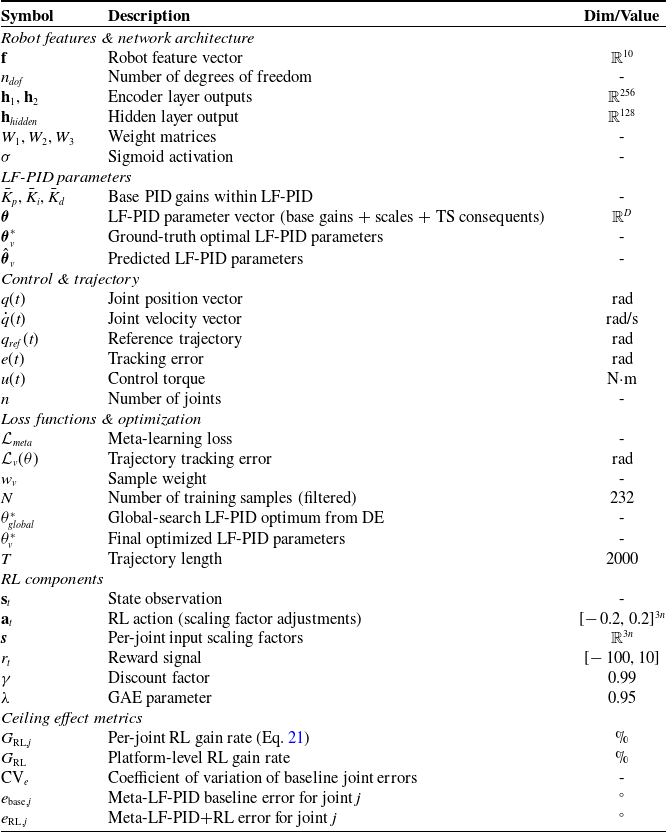

 f
 θ^=[K¯^,s^,c^]∈[0,1]D
 D=330n
 K¯∈R3n
 s∈R3n
 c∈Rdc
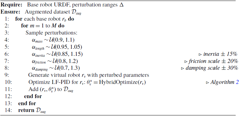
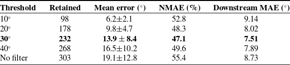
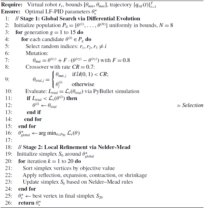

 Lv(θ∗)

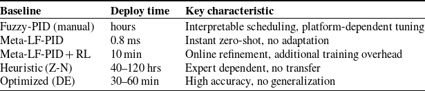
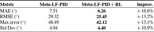
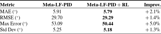

 12.36∘
 2.42∘
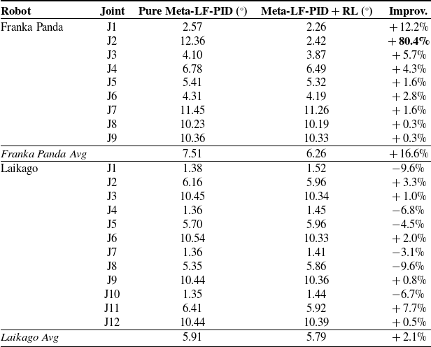


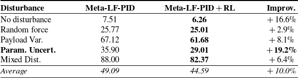
 ∘

 ±
 ±
 35.90∘
 29.01∘
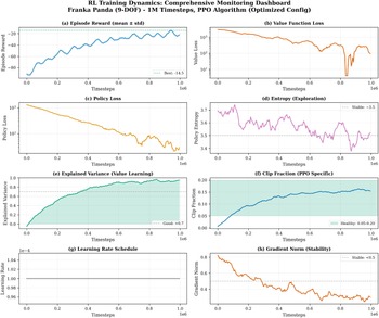
 1×10⁻⁴

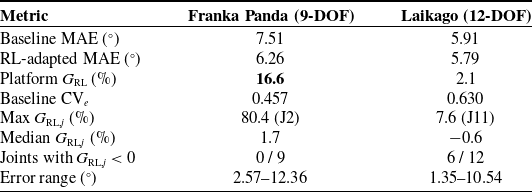
 GRL
 CVe
 GRL,j
 GRL,j<0

 GRL,j
 ebase,j
 GRL<5%
 ebase=12.36∘
 GRL=80.4%
 ρs=0.38
 n=21