1. Introduction
Total factor productivity (TFP) is considered the dominant factor accounting for income per capita differences across countries.Footnote 1 Instead of focusing on the inefficiency within a representative firm, a growing strand of the literature emphasizes the role of factor allocation efficiency across heterogeneous firms in explaining the observed aggregate TFP differences.Footnote 2 Furthermore, the well-documented strong positive correlation between financial development and aggregate TFPFootnote 3 has driven recent work examining the role of financial frictions.Footnote 4 In this line of research with imperfect financial markets, firms face the collateral-type borrowing constraint with homogeneous borrowing tightness.Footnote 5
However, empirical evidence suggests that firms’ financing ability depends largely on firm size, which is the fundamental firm characteristic. By analyzing the Chinese firm-level dataset for the period 1998-2007, I find that in the Chinese manufacturing sector, there exists a positive relationship between leverage and firm size among private firms. That is, large firms face lower borrowing tightness and tend to have higher leverage than small firms. Similar empirical evidence for the positive leverage-size slope can be found in Arellano et al. (Reference Arellano, Bai and Zhang2012), Gopinath et al. (Reference Gopinath, Kalemli-Özcan, Karabarbounis and Villegas-Sanchez2017), and Bai et al. (Reference Bai, Lu and Tian2018).Footnote 6 Since a firm’s financing ability directly affects its capital decisions, failing to take into account the financial frictions disciplined by the observed firms’ financing patterns may prevent salient features of capital misallocation from being captured.
This paper fills this gap by focusing on firms’ financing patterns and studies the impacts of size-dependent financial frictions on capital misallocation and aggregate productivity.Footnote 7 To capture the empirical fact that large firms have higher leverage than small firms, this paper builds a model of firm dynamics by incorporating the size-dependent borrowing constraint under which larger firms face lower borrowing tightness while enabling firms’ capital decisions to be analytically tractable.
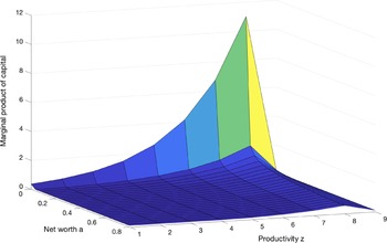
In the model, the optimal unconstrained capital level increases in productivity. Under the collateral constraint with a size-invariant maximum leverage, the marginal product of capital increases in productivity, since given a certain net worth level, firms with higher productivity have higher financing needs and are more likely to be constrained. By contrast, with the size-dependent borrowing constraint, as the maximum attainable leverage ratio increases with firm size, the relationship between the marginal product of capital and productivity becomes non-monotonic. When productivity is sufficiently high, firms, even those without high net worth, are able to accumulate adequate capital, grow large, and relax the borrowing constraint. With this feature, the marginal product of capital and productivity are less positively correlated and large firms are less impacted by financial frictions relative to the case under the homogeneous borrowing constraint.
To discipline the quantitative model, I document several facts on capital misallocation based on the Chinese firm-level dataset. Since policies may drive a wedge between factor prices and the marginal product of capital, the dispersion of the marginal product of capital as a measure of capital allocation efficiency is at the center of the analysis. First, the standard deviation of the marginal product of capital is persistent over the sample period, suggesting the existence of capital misallocation. In addition, non-state-owned enterprises (non-SOEs) face a higher dispersion of the marginal product of capital than state-owned enterprises (SOEs). Second, the extent to which firms are distorted varies across different firm size groups. The mean and dispersion of the marginal product of capital are smaller among large firms, suggesting that large firms are less distorted in capital decisions than their small counterparts. Regarding financing patterns, SOEs are not financially constrained, while non-SOEs have less access to bank loans and lower leverage. Moreover, a positive relationship between firm size and leverage exists for non-SOEs. The implications of size-dependent financial frictions faced by non-SOEs, under which large firms are more favored in financial market than small firms, are in line with the capital misallocation facts.
This paper quantifies the impacts of the size-dependent borrowing constraint on capital misallocation and the aggregate TFP in the Chinese manufacturing sector. The parameters are jointly calibrated to match the moments of the firm-level and aggregate data in China. In particular, the borrowing tightness parameters are set to match both financial development (the debt-to-GDP ratio) and firms’ financing pattern (the positive leverage-size slope). The model with the size-dependent borrowing constraint matches well the firms’ financing pattern, the skewed output distribution, and other non-targeted moments. Moreover, the model with the size-dependent borrowing constraint explains approximately 35% of the dispersion of the marginal product of capital. The rationale for this result is that there are other forces in addition to financial frictions that contribute to capital misallocation, consistent with the findings of existing empirical work on Chinese manufacturing firms.Footnote 8 This model also generates similar patterns of the mean and dispersion of the marginal product of capital across size groups as in the data.
This paper focuses on the mechanism of the observed negative correlation between firm size and the marginal product of capital. Under the homogeneous borrowing constraint, which corresponds to the size-invariant maximum leverage, the model fails to reproduce the negative correlation between firm size and the marginal product of capital, as the correlation equals zero. By contrast, under the size-dependent borrowing constraint, when the productivity shock is sufficiently large, firms without a high net worth are able to accumulate adequate capital, relax the borrowing constraint, and face a low marginal product of capital. Due to this feature, the positive correlation between the marginal product of capital and productivity is weaker, and large firms are less distorted than in the case under the homogeneous borrowing constraint. Hence, the model with the size-dependent borrowing constraint generates a negative correlation between firm size and the marginal product of capital with a coefficient of −0.16, consistent with the data (−0.23).
In the model with the size-dependent borrowing constraint, the aggregate TFP loss is 3.91%, which implies that size-dependent financial frictions explain modest TFP loss along the intensive margin.Footnote 9 One rationale for this result is that self-financing undoes the impacts of the borrowing constraint on capital misallocation to some extent under persistent productivity shocks, as discussed in Moll (Reference Moll2014). Under the homogeneous borrowing constraint, the TFP loss is instead 5.08%. This indicates that without considering the size-dependent financial frictions, we may not only fail to capture the relationship between firm size and misallocation but also overstate the TFP loss since large firms, which contribute most to the economy, are actually less financially constrained.
To examine the important role of the borrowing tightness parameter in the financing patterns of firms, this paper conducts a sensitivity analysis. As the value of the borrowing tightness parameter increases, which corresponds to a larger leverage-size slope, the positive correlation between productivity and the marginal product of capital becomes weaker, and the negative relationship between firm size and the marginal product of capital becomes stronger. The dispersion of the marginal product of capital and the TFP loss decrease accordingly. Moreover, compared with small firms, both the mean and dispersion of the marginal product of capital decrease further among large firms, suggesting that large firms benefit more from an increasing leverage-size slope than small firms.
This paper closely relates to the growing strand of literature studying the impacts of financial frictions on misallocation and aggregate productivity. Moll (Reference Moll2014) develops a general equilibrium model with a collateral constraint to study the impacts of financial frictions on capital misallocation and aggregate TFP. Midrigan and Xu (Reference Midrigan and Xu2014) study a two-sector growth model of firm dynamics and show that financial frictions reduce the aggregate TFP by restraining firms’ entry and technology adoption decisions, as well as by distorting capital allocation across existing firms. This paper differs from these previous works by considering firms’ financing patterns and incorporating the size-dependent borrowing constraint. This paper shows that not considering firms’ financing patterns may fail to capture the patterns of capital misallocation and overestimate the TFP loss. This paper is also closely related to Gopinath et al. (Reference Gopinath, Kalemli-Özcan, Karabarbounis and Villegas-Sanchez2017), which differs in that it studies the impacts of the decline in the real interest rate since the 1990s in South Europe on productivity and focuses on transitional dynamics. The present paper instead quantifies the impacts of size-dependent financial frictions on aggregate TFP at the steady state.
This paper is also related to the literature on firms’ financing patterns. Arellano et al. (Reference Arellano, Bai and Zhang2012) show that there is a positive relationship between firm size and the leverage ratio based on the European dataset and that the leverage of small firms relative to large firms grows as financial development increases. Bai et al. (Reference Bai, Lu and Tian2018) take firms’ financing patterns, for example, the positive leverage-size slope among Chinese private firms, into account and quantify the role of financial frictions in determining aggregate productivity. This paper differs from these works in the formulation of the borrowing constraint. In Arellano et al. (Reference Arellano, Bai and Zhang2012) and Bai et al. (Reference Bai, Lu and Tian2018), the borrowing limit is determined by considering the default risks of firms and the fixed cost of issuing loans. However, in Bai et al. (Reference Bai, Lu and Tian2018), the model with the endogenous borrowing constraint generates a slightly positive correlation between firm size and the marginal product of capital, which deviates from the Chinese data. In this paper, the model can reproduce the patterns of misallocation whereby both the mean and dispersion of the marginal product of capital are lower among large firms than their small counterparts.
This paper also relates to the empirical findings on misallocation. David and Venkateswaran (Reference David and Venkateswaran2019) study various sources of capital misallocation in both China and the USA, for example, capital adjustment costs, informational frictions, and firm-specific factors. They find that in China, adjustment costs and uncertainty play a modest role, while other idiosyncratic factors, both productivity or size-dependent and permanent, substantially contribute to misallocation. This paper focuses on one specific factor, size-dependent financial frictions, in capital misallocation. Ruiz-García (Reference Ruiz-García2021) finds that the average and dispersion of the marginal product of capital are higher for young, small, and high-productivity firms based on a firm-level dataset from Spain. This paper reports similar findings in China. Hsieh and Olken (Reference Hsieh and Olken2014) instead show that bigger firms have a higher average product of capital in India, Indonesia, and Mexico. However, their empirical findings are based on a dataset that includes both formal and informal firms. The present paper differs in focusing on the formal Chinese manufacturing sector.
The rest of this paper is organized as follows. Section 2 presents the firm-level dataset of the Chinese manufacturing sector. Section 3 introduces the model and discusses the implications of the size-dependent financial frictions on capital misallocation. Section 4 presents the model parameterization, and Section 5 analyzes the simulation results. Section 6 concludes the paper.
2. Data
This section describes the data and presents the empirical findings on capital misallocation in the Chinese manufacturing sector. Strong evidence for the relationship between firm size and the marginal product of capital as well as firms’ financing patterns is found, which motivates the study of the impacts of size-dependent financial frictions on capital misallocation.
2.1. Data description
The empirical findings are based on the firm-level dataset for the period 1998-2007 from the Chinese Annual Survey of Industrial Firms. This dataset includes all SOEs and the “above-scale” non-SOEs with annual sales above 5 million RMB (approximately 700,000 US dollars). Firms in this dataset account for the top 20% of manufacturing firms by industrial sales and contribute to more than 90% of the total industrial output in China. This dataset reports abundant firm-level information and has been extensively studied in the existing literature related to Chinese firm behaviors.
To construct a panel for analysis purposes, I restrict the sample to the manufacturing sector and drop observations with negative key variables and observations with key variables that are not consistent with accounting standards.Footnote 10 Following Brandt et al. (Reference Brandt, Van Biesebroeck and Zhang2014), this paper creates a unique ID for each firm and constructs panel data based on the firm ID information. The output is measured by the value added and deflated by the GDP deflator. Following Brandt et al. (Reference Brandt, Van Biesebroeck and Zhang2014), capital is constructed by using the perpetual inventory method. Assets are measured by total assets, which serves as a proxy of firm size in this paper. To control differences in labor quality, labor is measured by the sum of wages and benefits and is then deflated by the CPI. Debt is measured by the sum of long-term and short-term debt. Leverage is defined as the ratio of total debt to total assets. The marginal product of capital is approximated by the average product of capital, which is the ratio of output to capital.
This paper further divides firms into SOEs and non-SOEs according to firm ownership since non-SOEs and SOEs in China are subject to different regulations. Following Hsieh and Song (Reference Hsieh and Song2015), I identify firms’ ownership by using the registered capital ratio. If the ratio of registered capital from the state to total registered capital is at least 50%, the firm is recognized as an SOE. Otherwise, the firm is a non-SOE. See Appendix A.1 for details.
2.2. Capital misallocation
The marginal product of capital is at the center of the analysis. In the absence of distortions, the marginal product of capital across firms should be equal, and more resources are allocated to firms that are more productive. However, policies or institutions may drive a wedge between the factor prices and marginal products.Footnote 11 Thus, the dispersion of the marginal product of capital helps to measure the capital allocation efficiency. Intuitively, as discussed in Midrigan and Xu (Reference Midrigan and Xu2014), the aggregate TFP loss is proportional to the dispersion of the marginal product of capital.
The standard deviation of
 $log(MP_{k})$
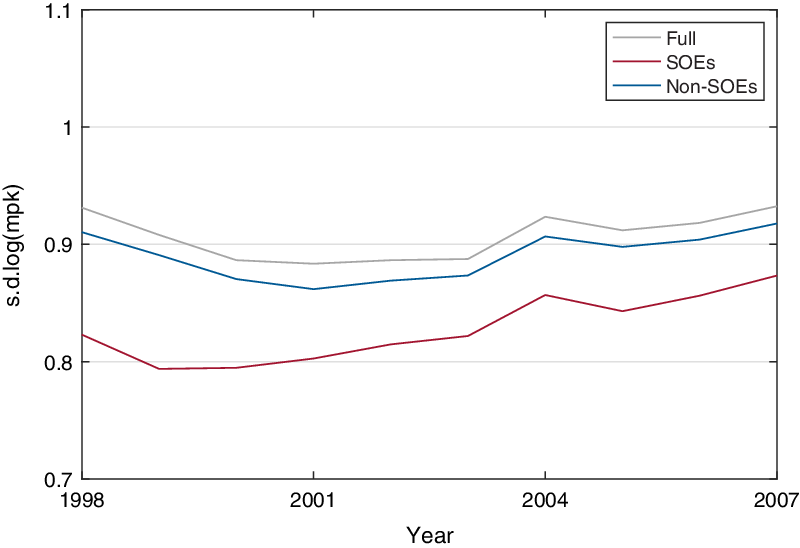
is obtained at the 4-digit industry level and then aggregated conditional on year. Figure 1 reports the evolution of the standard deviation of
 $log(MP_{k})$
over the period 1998-2007 for SOEs, non-SOEs, and the full sample. The dispersion of
 $log(MP_{k})$
among SOEs increases after 1999, and the average is 0.82. In comparison, the dispersion of
 $log(MP_{k})$
among non-SOEs is higher than SOEs over time, and the average is 0.89. Since SOEs and non-SOEs differ in their capital allocation efficiency, the dispersion of
 $log(MP_{k})$
for the full sample over time is even larger, with a mean of 0.91. The above results suggest the presence of capital misallocation among Chinese manufacturing firms over the sample period, and non-SOEs face larger distortions than SOEs. In addition, since SOEs compose only a minor fraction of the dataset (approximately 10% of the observations), the dispersion of
 $log(MP_{k})$
among non-SOEs and the full sample are quite close.
Dispersion of
 $log(MP_{k})$
by year
Note: This figure reports the standard deviation of
 $log(MP_{k})$
for SOEs, non-SOEs, and the full sample by year.

Policy distortions may drive capital misallocation through firm characteristics. In empirical corporate finance, firm size is a fundamental firm characteristic.Footnote
12
Next, I will examine how
 $log(MP_{k})$
varies across different size groups. I obtain the mean of
 $log(MP_{k})$
and the standard deviation of
 $log(MP_{k})$
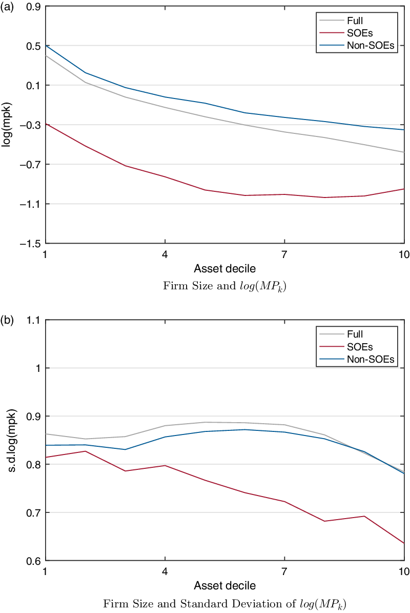
at the industry level and then aggregate them conditional on firm size. Firms are divided according to asset deciles. Figure 2 panel (a) shows the relationship between firm size and
 $log(MP_{k})$
. As we can see,
 $log(MP_{k})$
decreases with firm size for non-SOEs, suggesting that large firms are less distorted in investment decisions than their small counterparts. For SOEs,
 $log(MP_{k})$
decreases with firm size first and then increases for the top 20% of firms by assets. Furthermore, SOEs face lower
 $log(MP_{k})$
than non-SOEs across different firm sizes.
Firm size and
 $log(MP_{k})$
Note: This figure reports the relationship between firm size and
 $log(MP_{k})$
for SOEs, non-SOEs, and the full sample. The mean and standard deviation of
 $log(MP_{k})$
are calculated in each asset decile.

Figure 2 panel (b) presents the variation of the dispersion of
 $log(MP_{k})$
by firm size. The standard deviation of
 $log(MP_{k})$
among SOEs decreases with firm size and is lower than non-SOEs in each asset decile. The standard deviation of
 $log(MP_{k})$
among non-SOEs is close to that for the full sample, and it is smaller among large firms, suggesting lower capital misallocation among large firms than small firms.
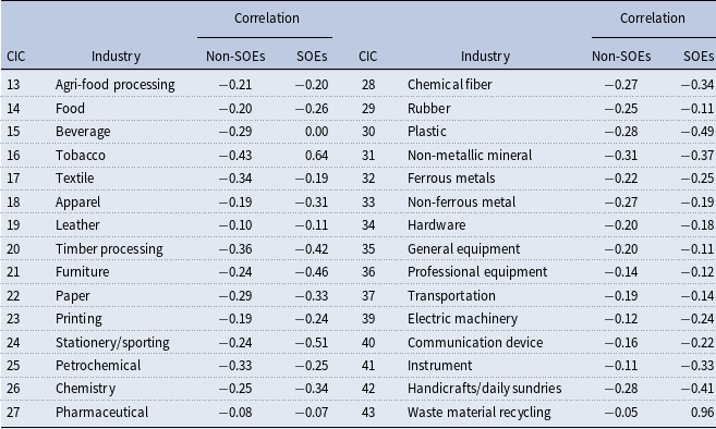
To further examine the relationship between
 $log(MP_{k})$
and firm size, I obtain the correlation between firm size and
 $log(MP_{k})$
by industry separately for non-SOEs and SOEs. There are thirty 2-digit industries in the manufacturing sector according to the industry concordances provided by Brandt et al. (Reference Brandt, Van Biesebroeck and Zhang2014).Footnote
13
As shown in Table 1, the correlation between firm size and
 $log(MP_{k})$
varies across different industries by ownership. A negative correlation exists in each industry for non-SOEs. For SOEs, except for the beverage, tobacco, and waste material recycling industries, firm size and
 $log(MP_{k})$
are negatively correlated.
Correlation between firm size and
 $log(MP_{k})$
by industry

Note: This table reports the correlation between firm size and
 $log(MP_{k})$
by the 2-digit industries. CIC denotes the China Industry Classification Code.
2.3. Financing patterns
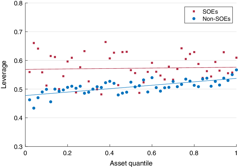
Financial frictions play a role in capital misallocation through firms’ characteristics, on which firms’ financing patterns depend. To see how the leverage ratio varies across different size groups, I calculate the average of leverage by asset quantiles separately for SOEs and non-SOEs, which is shown in Figure 3. First, credit discrimination exists in the Chinese credit market across firms of different ownership types. As Figure 3 shows, SOEs have a higher leverage ratio than non-SOEs, since the banking system, which is dominated by the four state-owned banks, tends to lend to SOEs instead of non-SOEs, which lack political connections. The result is consistent with existing literature. For example, Dollar and Wei (Reference Dollar and Wei2007) and Song et al. (Reference Song, Storesletten and Zilibotti2011) report that SOEs rely more on domestic bank loans to finance investments than non-SOEs. Poncet et al. (Reference Poncet, Steingress and Vandenbussche2010) and Curtis (Reference Curtis2016) also suggest that private Chinese firms are credit-constrained, while SOEs are not.
Second, SOEs and non-SOEs demonstrate different financing patterns. As Figure 3 shows, the leverage ratio of firms fluctuates with firm size, and large non-SOEs tend to have a higher leverage ratio than their small counterparts with an upward-sloping fitted line. In contrast, SOEs do not demonstrate a size-dependent leverage trend. Similarly, Boyreau-Debray and Wei (Reference Boyreau-Debray and Wei2005) also suggest that all types of banks prefer to lend to SOEs and large private firms in China.
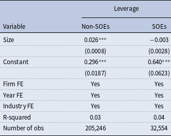
To further compare the financing patterns between SOEs and non-SOEs, this paper examines the relationship between firm size and leverage by regression. The regression model is given by the following:
 \begin{equation} lev_{ict}=\beta _{0}+\beta _{1}size_{ict}+dummy+u_{ict} \end{equation}
where
 $i$
denotes the firm,
 $c$
denotes the 4-digit industry, and
 $t$
denotes the year. The dependent variable is leverage and measured by the debt-to-asset ratio.
 $size_{ict}$
is measured by the logarithm of total assets. The term dummy includes the fixed effects of firm, year, and 4-digit industry. Moreover,
 $u_{ict}$
is the error term. Table 2 reports the regression results of leverage on firm size separately for non-SOEs and SOEs. The leverage-size slope among non-SOEs is 0.026 and significant, implying that leverage increases with firm size within non-SOEs, consistent with the existing literature. In addition, the regression coefficient of leverage on firm size is insignificantly −0.003 among SOEs, suggesting that firm size has no statistically significant relationship with leverage for those firms.
Regression coefficients of leverage on firm size
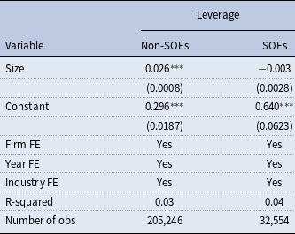
Note: This table reports the regression results for leverage on firm size separately for non-SOEs and SOEs. ***, **, and * denote results significantly different from zero at the 1%, 5%, and 10% levels. Standard errors are in parentheses.
Firm size and leverage
Note: This figure reports the relationship between firm size and leverage for SOEs, non-SOEs, and the full sample. The mean leverage ratio is calculated in each asset quantile (50 quantiles).

Recap. The above evidence suggests the presence of capital misallocation among Chinese manufacturing firms. Since SOEs have easy access to external finance and are not financially constrained, the dispersion of the marginal product of capital and the negative relationship between firm size and the marginal product of capital among those firms may mainly be attributed to factors other than financial frictions. In contrast, non-SOEs face a more significant dispersion of the marginal product of capital and have less access to bank loans and lower leverage than SOEs. Moreover, large non-SOEs face both a lower marginal product of capital and higher leverage than their small counterparts. Because firms’ financing ability directly affects their capital decisions, the remainder of the paper will mainly focus on non-SOEs. I will examine how the financial frictions driven by firms’ financing patterns, which correspond to the size-dependent financial frictions, explain the observed patterns of capital misallocation among non-SOEs.
Since the presence of SOEs also contributes to the dispersion of the marginal product of capital, capital misallocation and TFP loss will be underestimated when only considering non-SOEs. Nonetheless, as discussed in Section 2.2, since SOEs account for only a minor fraction of the data, the dispersion of the marginal product of capital for non-SOEs is quite close to that of the full sample. This indicates that the majority of capital misallocation and TFP loss in China’s manufacturing industry results from the distortions faced by non-SOEs.
3. The model
This section provides a general equilibrium model with heterogeneous agents based on Midrigan and Xu (Reference Midrigan and Xu2014) and incorporates a size-dependent borrowing constraint in light of Gopinath et al. (Reference Gopinath, Kalemli-Özcan, Karabarbounis and Villegas-Sanchez2017). The economy is populated by a continuum of firms and a unit measure of workers. Firms are exogenously heterogeneous in their productivity and can finance investment through both internal funds and external borrowing. The amount of debt that firms can issue is limited, and the maximum attainable leverage increases in firm size.
3.1. Firms
Technology. There is a continuum of firms indexed by
 $i$
that adopt both labor
 $l_{it}$
and capital
 $k_{it}$
to produce homogeneous goods
 $y_{it}$
subject to a decreasing-return-to-scale technology. The production function for firm
 $i$
is given by
 \begin{equation} y_{it}=z_{it}^{1-\eta }\!\left(l_{it}^{\alpha }k_{it}^{1-\alpha }\right)^{\eta } \end{equation}
where
 $\eta$
governs the span of control, which measures the degree of diminishing return to scale at the firm level as in Lucas (Reference Lucas1978);
 $\alpha$
is the labor elasticity. The idiosyncratic productivity shock
 $z_{it}$
is independently and identically distributed across firms and follows a Markov switching process.
Timing. Time is discrete. Following Moll (Reference Moll2014) and Midrigan and Xu (Reference Midrigan and Xu2014), exogenous productivity shocks
 $z_{it+1}$
are known to firms at the end of period
 $t$
. Firms borrow
 $d_{it+1}$
to finance capital
 $k_{it+1}$
according to the new productivity
 $z_{it+1}$
.Footnote
14
This convenient assumption makes capital measurable to productivity, and it enables this paper to focus on capital misallocation due to financial frictions.Footnote
15
In each period, firms choose consumption
 $c_{it}$
, labor
 $l_{it}$
, capital
 $k_{it+1}$
, and debt
 $d_{it+1}$
. Firm
 $i$
maximizes the present discounted lifetime utility:
 \begin{equation} \max _{\left \{ c_{it}, l_{it}, k_{it+1}, d_{it+1}\right \} _{t=0}^{\infty }}E_{0}\sum _{t=0}^{\infty }\beta ^{t}log(c_{it}) \end{equation}
subject to the budget constraint given by
 \begin{equation} c_{it}+k_{it+1}-(1-\delta )k_{it}=y_{it}-W l_{it}-(1+r)d_{it}+d_{it+1} \end{equation}
where
 $\beta$
is the discount factor,
 $W$
is the real wage per efficiency unit of labor, and
 $r$
is the real interest rate.
Size-dependent borrowing constraint. Considering the empirical fact that large firms tend to face lower borrowing tightness and have higher leverage than small firms, following Gopinath et al. (Reference Gopinath, Kalemli-Özcan, Karabarbounis and Villegas-Sanchez2017), the size-dependent borrowing constraint is introduced into this paper,
 \begin{equation} d_{it+1}\leq \theta _{0}k_{it+1}+\theta _{1}\Phi (k_{it+1}) \end{equation}
where parameters
 $\theta _{0}$
and
 $\theta _{1}$
jointly govern the borrowing tightness. The borrowing constraint arises because the contract has limited enforceability, and borrowers can choose to default. In the event of default, a firm reneges on a fraction
 $\mu _{0}$
of its debt
 $d_{it+1}$
; as a penalty, the bank seizes a fraction
 $\mu _{1}$
of the undepreciated capital
 $(1-\delta )k_{it+1}$
. In addition, there is a disruption cost
 $\Phi (k_{it+1})$
that the firm has to pay at default, which may arise due to a loss of suppliers, market share, reputation, etc. In equilibrium, banks extend their credit only to the extent that no firm will renege on the contract. Therefore, the amount of debt that the firm can borrow is limited. The default-deterring borrowing limit satisfying the incentive compatibility constraint is endogenously given by the forgone revenues of firms at default. The derivation of the borrowing constraint is shown in Appendix B.1.Footnote
16
Considering that larger firms lose more in the event of default, the disruption cost
 $\Phi (k)$
is assumed to be an increasing and convex function of capital
 $k$
.Footnote
17
Because the disruption costs increase in capital, it is more costly for large firms to default than small firms, which makes debt redemption more valuable and relaxes the borrowing limit in the no-default equilibrium as firm size increases. The functional form of the disruption costs is assumed to be
 $\Phi (k)=k^{2}$
, which is analytically convenient in obtaining a closed-form solution for capital. The borrowing tightness, which corresponds to the maximum attainable leverage ratio
 $(d/k)_{max}$
, is
 \begin{equation} \left (d/k\right )_{max}=\theta _{0}+\theta _{1}k \end{equation}
If
 $\theta _{1}=0$
, all firms face a single borrowing tightness. As long as
 $\theta _{1}$
is positive, the maximum attainable leverage
 $(d/k)_{max}$
is an increasing function of capital
 $k$
, which implies that large firms will face lower borrowing tightness than small firms. Since the borrowing constraint nests the most studied constraint with the size-invariant borrowing tightness as in Moll (Reference Moll2014) and Buera and Moll (Reference Buera and Moll2015), it facilitates the comparison of the size-dependent borrowing constraint with the existing literature and also simplifies some of the computation. In the rest of the paper, I call the borrowing constraint the homogeneous borrowing constraint if
 $\theta _{1}=0$
and the size-dependent borrowing constraint if
 $\theta _{1}\gt 0$
. I compare the implications of the two cases. Additionally, there may exist alternative specifications of size-dependent borrowing constraints, for example, borrowing constraint with size-dependent pledgeability and earnings-based borrowing constraint, that also account for the cross-sectional moments in the data. The alternative borrowing constraints are discussed in Appendix C.
Recursive formulation. Using
 $a=k-d\geq 0$
to denote the net worth and primes to indicate next-period variables, the optimization problem of a firm can be written in the following recursive form
 \begin{equation} V(a,z)=\max _{a^{\prime},c}log(c)+\beta EV\!\left(a^{\prime},z^{\prime}\right) \end{equation}
subject to the budget constraint given by
 \begin{equation} c+a^{\prime}=\pi +(1+r)a \end{equation}
and the borrowing constraint, which can be rewritten as
 \begin{equation} k^{\prime}\leq \lambda _{0}a^{\prime}+\lambda _{1}k^{\prime 2} \end{equation}
where the firm solves the static profit maximization problem
 \begin{equation} \pi (a,z) = \max _{k,l}z^{1-\eta }(l^{\alpha }k^{1-\alpha })^{\eta }-W l-(r+\delta )k \end{equation}
 \begin{equation} s.t.\quad k\leq \lambda _{0}a+\lambda _{1}k^{2} \end{equation}
Note that
 $\lambda _{0}=\frac{1}{1-\theta _{0}}$
and
 $\lambda _{1}=\frac{\theta _{1}}{1-\theta _{0}}$
. A larger
 $\lambda _{1}$
(or a smaller
 $\lambda _{0}$
) corresponds to a higher leverage-size slope. When
 $\theta _{1}=0$
,
 $\lambda _{1}=0$
accordingly, which implies that firms face homogeneous borrowing tightness. The parameter restrictions placed on the borrowing constraint are
 $\lambda _{0}\geq 1$
and
 $\lambda _{1}\geq 0$
. Appendix B.2 presents the derivation of the parameter restrictions. Given a net worth
 $a$
and productivity
 $z$
, the firm maximizes its profit by choosing labor
 $l$
and capital
 $k$
subject to the borrowing constraint in equation (11).Footnote
18
Then, the firm chooses consumption
 $c$
and net worth
 $a^{\prime}$
subject to the budget constraint in equation (8) and the borrowing constraint in equation (9).
The Euler equation can be solved as
 \begin{equation} \frac{1}{c(a,z)}=\beta E\!\left\{ \frac{1}{c\!\left(a^{\prime},z^{\prime}\right)}\left [\left (1+r\right )+\mu\!\left(a^{\prime},z^{\prime}\right)\lambda _{0}\right ]\right \} \end{equation}
where
 $\mu (a,z)$
is the Lagrangian multiplier on the borrowing constraint. Since
 $a^{\prime}$
appears in the borrowing constraint in equation (9), the expectation of a binding borrowing constraint increases the net worth accumulation. Firms with high productivity tend to accumulate net worth, since productivity is persistent and firms expect a high demand for capital in the future. In addition, firms with low net worth also tend to accumulate internal funds.
Firms choose labor
 $l$
and capital
 $k$
to maximize their profit subject to the borrowing constraint in equation (11).
 $FOCs$
with respect to labor
 $l$
and capital
 $k$
are given by
 \begin{equation} \alpha \eta \frac{y(a,z)}{l(a,z)}=W \end{equation}
 \begin{equation} \left (1-\alpha \right )\eta \frac{y(a,z)}{k(a,z)}=r+\delta +\mu (a,z)\!\left [1-2\lambda _{1}k(a,z)\right ] \end{equation}
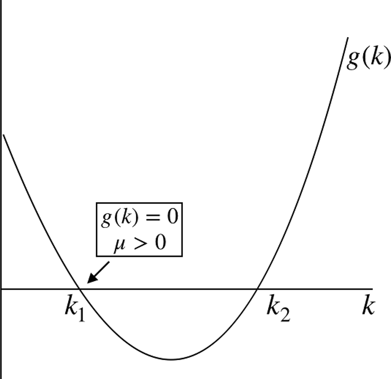
Capital decisions. Firms’ capital decisions depend on both their productivity and financing ability. To obtain a closed-form solution of capital for financially constrained firms, I define the function
 $g(k)$
as the difference between the right-hand side and the left-hand side of the borrowing constraint in equation (11):
 \begin{equation} g(k)\equiv \lambda _{0}a+\lambda _{1}k^{2}-k \end{equation}
When the borrowing constraint is binding,
 $g(k)=0$
. The solution to
 $g(k)=0$
is
 \begin{equation} k_{1,2}=\frac{1\pm \sqrt{1-4\lambda _{0}\lambda _{1}a}}{2\lambda _{1}},\;where\;k_{1}\leq k_{2} \end{equation}
The number of roots depends on the values of the borrowing tightness parameters
 $\lambda _{0}$
and
 $\lambda _{1}$
and the net worth
 $a$
.
Proposition 1. Under the size-dependent borrowing constraint, the capital decisions for the financially unconstrained and constrained firms are as follows:
-
1) When the borrowing constraint is slack, firms can achieve the optimal capital level
 $k^{u}$
:
(17)
\begin{equation} k^{u}=\left(\frac{\alpha \eta }{W}\right)^{\frac{\alpha \eta }{1-\eta }}\!\left(\frac{(1-\alpha )\eta }{r+\delta }\right)\!^{\frac{1-\alpha \eta }{1-\eta }} z \end{equation}
-
2) When the borrowing constraint is binding, firms can achieve a capital level of only
$k^{c}$
:
(18)
\begin{equation} k^{c}=\frac{1-\sqrt{1-4\lambda _{0}\lambda _{1}a}}{2\lambda _{1}},\quad and\quad k^{c}\leq k^{u} \end{equation}


Proof. See Appendix B.3.
According to Proposition 1, the optimal unconstrained level of capital
 $k$
increases in productivity
 $z$
; the constrained level of capital
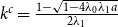 $k^{c}=\frac{1-\sqrt{1-4\lambda _{0}\lambda _{1}a}}{2\lambda _{1}}$
depends on net worth
 $a$
. Since
 $k^{c}\leq k^{u}$
, the investment of financially constrained firms is insufficient. By comparison, under the homogeneous borrowing constraint (
 $\lambda _{1}=0$
), the optimal unconstrained capital decision is also
 $k^{u}=z\left(\frac{\alpha \eta }{W}\right)^{\frac{\alpha \eta }{1-\eta }}((1-\alpha )\eta )^{\frac{1-\alpha \eta }{1-\eta }}(r+\delta )^{\frac{\alpha \eta -1}{1-\eta }}$
; when the borrowing constraint is binding, the attainable capital level is
 $k^{c}=\lambda _{0}a$
, which is linear in net worth
 $a$
.
Firms are heterogeneous in their dependence on debt, and in each period, the borrowing constraint is binding only for some firms. The bindingness of the borrowing constraint depends on both firms’ productivity and net worth and is different under the homogeneous borrowing constraint (
 $\lambda _{1}=0$
) and the size-dependent borrowing constraint (
 $\lambda _{1}\gt 0$
), which is discussed as follows.
Proposition 2.
Under the homogeneous borrowing constraint, given productivity
 $z$
, the cutoff net worth for the bindingness of the borrowing constraint is
 $a^{*}=\frac{k^{u}(z)}{\lambda _{0}}$
. When
 $a\leq{a^{*}}$
, the borrowing constraint is binding; when
 $a\gt \frac{k^{u}(\bar{z})}{\lambda _{0}}$
, the borrowing constraint is never binding.
Proof. See Appendix B.4.
Proposition 3.
Under the size-dependent borrowing constraint, given productivity
 $z$
, the cutoff net worth for the bindingness of the borrowing constraint is
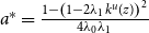 $a^{*}=\frac{1- \left (1-2\lambda _{1}k^{u}(z)\right )^{2}}{4\lambda _{0}\lambda _{1}}$
. When
 $a\leq{a^{*}}$
, the borrowing constraint is binding; when
 $a\gt \frac{1}{4\lambda _{0}\lambda _{1}}$
, the borrowing constraint is never binding.
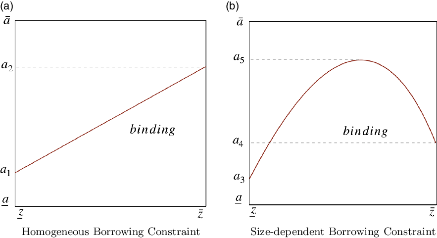
Bindingness of the borrowing constraint
Note: This figure depicts the bindingness of the borrowing constraint. For firms with state
 $(a,z)$
below the red line, the borrowing constraint is binding.

Proof. See Appendix B.5.
Figure 4 reports the bindingness of the homogeneous borrowing constraint and the size-dependent borrowing constraint, respectively. The red line denotes the cutoff net worth
 $a^{*}$
for bindingness. In Figure 4 Panel (a),
 $a_{1}=\frac{k^{u}(\underline{z})}{{{\lambda _{0}}}}$
and
 $a_{2}=\frac{k^{u}(\bar{z})}{{{\lambda _{0}}}}$
. Under the homogeneous borrowing constraint, the cutoff net worth
 $a^{*}=\frac{k^{u}(z)}{\lambda _{0}}$
increases fully with productivity
 $z$
. That is, since firms with higher productivity
 $z$
have a higher financing need for capital, the required net worth should be larger to not be constrained. Figure 4 Panel (b) shows the bindingness of the size-dependent borrowing constraint. In this figure,
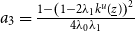 $a_{3}=\frac{1-\left (1-2\lambda _{1}k^{u}(\underline{z})\right )^{2}}{4\lambda _{0}\lambda _{1}}$
,
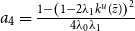 $a_{4}=\frac{1-\left (1-2\lambda _{1}k^{u}(\bar{z})\right )^{2}}{4\lambda _{0}\lambda _{1}}$
, and
 $a_{5}=\frac{1}{4\lambda _{0}\lambda _{1}}$
. Notably, the cutoff net worth
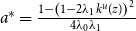 $a^{*}=\frac{1-\left (1-2\lambda _{1}k^{u}(z)\right )^{2}}{4\lambda _{0}\lambda _{1}}$
is non-monotonic in productivity. That is, when productivity
 $z$
is sufficiently large, capital
 $k^{u}$
with respect to productivity will be high, which in turn enables those firms (even without high net worth) to relax the borrowing constraint. By contrast, under the homogeneous borrowing constraint, which corresponds to a size-invariant maximum leverage, firms with large productivity
 $z$
are more likely to be financially constrained.
Marginal product of capital. As financially constrained firms cannot fully adjust capital to the efficient level in response to the productivity shock, dispersion of
 $MP_{k}$
endogenously arises across firms. The determination of the marginal product of capital is different under the homogeneous borrowing constraint and the size-dependent borrowing constraint.
Proposition 4. Under the homogeneous borrowing constraint,
-
1) Given productivity shock
$z$
, financially constrained firms with higher net worth
$a$
face a lower
$MP_{k}$
; financially unconstrained firms face a constant
$MP_{k}=r+\delta$
. -
2) Given net wealth
$a$
, financially unconstrained firms with higher productivity
$z$
face a constant
$MP_{k}=r+\delta$
; financially constrained firms with higher productivity
$z$
face a higher
$MP_{k}$
.


Proof. See Appendix B.6.
As discussed above, let
 $a_{1}=\frac{k^{u}(\underline{z})}{{{\lambda _{0}}}}$
,
 $a_{2}=\frac{k^{u}(\bar{z})}{{{\lambda _{0}}}}$
, the cutoff net worth
 $a^{*}$
for bindingness given productivity
 $z$
be
 $\frac{k^{u}(z)}{\lambda _{0}}$
, and the cutoff productivity for bindingness given net worth
 $a$
be
 $z^{*}$
. Given productivity
 $z$
, when
 $a\in \left [\underline{a},a^{*}\right ]$
, firms are constrained. Firms with larger net worth face a lower
 $MP_{k}$
. Given net worth
 $a\in (a_{1},a_{2}]$
, when productivity
 $z\in [\underline{z},z^{*})$
, firms are unconstrained and
 $MP_{k}=r+\delta$
; when productivity becomes large, for example,
 $z\in \left [z^{*},\bar{z}\right ]$
, firms are constrained, and firms with higher productivity face a higher
 $MP_{k}$
. Further details can be seen in Appendix B.6. Overall, with the homogeneous borrowing constraint, given productivity, firms with higher net worth are less likely to be constrained and tend to face a lower
 $MP_{k}$
. Given net wealth, firms with higher productivity are more likely to be constrained and face a higher
 $MP_{k}$
.
Proposition 5. Under the size-dependent borrowing constraint,
-
1) Given productivity shock
$z$
, financially constrained firms with higher net worth
$a$
face a lower
$MP_{k}$
; financially unconstrained firms face a constant
$MP_{k}=r+\delta$
. -
2) Given net wealth
$a$
, financially unconstrained firms with higher productivity
$z$
face a constant
$MP_{k}=r+\delta$
; financially constrained firms with higher productivity
$z$
face a higher
$MP_{k}$
. -
3) Firms with sufficiently large productivity shock
$z$
are financially unconstrained and face a constant
$MP_{k}=r+\delta$
.


Proof. See Appendix B.7.
As discussed in Proposition 3, let
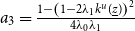 $a_{3}=\frac{1-\left (1-2\lambda _{1}k^{u}(\underline{z})\right )^{2}}{4\lambda _{0}\lambda _{1}}$
,
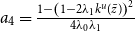 $a_{4}=\frac{1-\left (1-2\lambda _{1}k^{u}(\bar{z})\right )^{2}}{4\lambda _{0}\lambda _{1}}$
,
 $a_{5}=\frac{1}{4\lambda _{0}\lambda _{1}}$
, the cutoff net worth
 $a^{*}$
for bindingness given productivity
 $z$
be
 $\frac{1-\left (1-2\lambda _{1}k^{u}(z)\right )^{2}}{4\lambda _{0}\lambda _{1}}$
, and the cutoff productivities for bindingness given net worth
 $a$
be
 $z^{*}_{1}$
and
 $z^{*}_{2}$
. Different from the homogeneous borrowing constraint, the relationship between productivity and the marginal product of capital now is non-monotonic. That is, given net worth
 $a\in (a_{4},a_{5}]$
, when
 $z\in \left [z^{*}_{1}, z^{*}_{2}\right ]$
, firms are constrained; firms with higher productivity
 $z$
face a higher
 $MP_{k}$
. However, when productivity is sufficiently large, for example,
 $z\in (z^{*}_{2}, \bar{z}]$
, firms even without high net worth
 $a$
are financially unconstrained. This is because those highly productive firms will accumulate sufficient capital, which in turn enables them to relax the borrowing constraint and face a low
 $MP_{k}$
. Further details are given in Appendix B.7.
3.2. Workers
There is a unit measure of workers in the economy. Following Midrigan and Xu (Reference Midrigan and Xu2014), workers differ in their idiosyncratic efficiency
 $v_{it}$
, which follows a two-state Markov process. Each worker supplies
 $v_{it}$
efficiency units of labor in period
 $t$
. They cannot borrow and only save by holding risk-free asset
 $a_{it+1}^{w}$
. Workers also have log preference
 $log(c^{w}_{it})$
as firms do. Using primes to indicate next-period variables, the optimization problem of a worker can be written in the following recursive form:
 \begin{equation} V^{w}(a^{w},v)=\max _{c^{w},a^{w^{\prime}}}log(c^{w})+\beta EV^{w}\!\left(a^{w^{\prime}},v^{\prime}\right) \end{equation}
subject to the budget constraint that
 \begin{equation} c^{w}+a^{w^{\prime}}=W v+(1+r)a^{w} \end{equation}
As workers are heterogeneous in their labor efficiency
 $v_{it}$
, they are also different in their asset holdings
 $a_{it}^{w}$
, which are endogenously determined in the model.
3.3. Equilibrium
A recursive competitive equilibrium consists of value functions
 $V^{w}(a^{w},v)$
for workers, and
 $V(a,z)$
for firms; policy functions
 $c^{w}(a^{w},v),a^{w^{\prime}}(a^{w},v)$
for workers, and
 $c(a,z),a^{\prime}(a,z)$
for firms; output
 $y(a,z)$
, labor
 $l(a,z)$
, and capital
 $k(a,z)$
for firms; a stationary probability distribution
 $n(a,z)$
for firms; constant factor prices
 $W$
and
 $r$
, and aggregate variables, such that:
-
1. Given factor prices
$W$
and
$r$
, the value functions and decision rules solve the workers’ and firms’ optimization problems; -
2. Markets clear
-
(i) Labor market
(21)
\begin{equation} L=\int _{A}\int _{Z}l(a,z)dn(a,z) \end{equation}
-
(ii) Asset market
(22)
\begin{equation} A^{w^{\prime}}+\int _{A}\int _{Z} a^{\prime}(a,z)dn(a,z)=\int _{A}\int _{Z} k^{\prime}(a,z)dn(a,z) \end{equation}
-
(iii) Goods market
(23)
\begin{equation} C+I=Y \end{equation}
where
$Z= \left [\underline{z},\bar{z}\right ]$
and
$A=\left [\underline{a},\bar{a}\right ]$
are sets of productivity and net worth values.
$L$
is the aggregate efficiency units of labor supplied by workers.
$A^{w^{\prime}}$
is the aggregate asset holdings by workers.
$C$
is the aggregate consumption, which is the sum of consumption by firms and workers.
$I$
and
$Y$
are the aggregate investment and output, respectively. -
-
3. The distribution
$n(a,z)$
over state
$\left (a,z\right )$
is stationary, which is induced via the exogenous Markov chain for productivity
$z$
and policy function for net worth
$a^{\prime}(a,z)$
.


In the model, the exogenous productivity process and the policy function for the net worth
 $a^{\prime}(a,z)$
jointly determine the endogenous Markov chain for
 $(a,z)$
pairs on the state-space
 $A\times Z$
. This “big” Markov chain has a stationary distribution
 $n(a,z)$
. In the stationary equilibrium, firms’ choices fluctuate over time in response to productivity shocks, whereas the aggregate variables and prices are constant.
3.4. TFP loss
Since firms produce homogeneous goods, by integrating the output across firms, I obtain the aggregate production function given by
 \begin{equation} Y=\frac{\left (\int _{i} z_{i}MP_{ki}{}^{-\frac{\left (1-\alpha \right )\eta }{1-\eta }}di\right )^{\!1-\alpha \eta }}{\left (\int _{i} z_{i}MP_{ki}{}^{\frac{\alpha \eta -1}{1-\eta }}di\right )^{\!\left (1-\alpha \right )\eta }}(L^{\alpha }K^{1-\alpha })^{\eta } \end{equation}
The aggregate measured TFP is then defined as
 \begin{equation} TFP = \frac{\left (\int _{i} z_{i}MP_{ki}{}^{-\frac{\left (1-\alpha \right )\eta }{1-\eta }}di\right )^{\!1-\alpha \eta }}{\left (\int _{i} z_{i}MP_{ki}{}^{\frac{\alpha \eta -1}{1-\eta }}di\right )^{\!{\left (1-\alpha \right )\eta }}} \end{equation}
which is endogenously determined by the firm-level productivity and the extent to which firms are financially constrained. Given the same amount of aggregate capital and labor, without financial frictions, resources are allocated efficiently. Then, the first-best aggregate TFP is
 \begin{equation} TFP^{e}=\left (\int _{i} z_{i}di\right )^{\!1-\eta } \end{equation}
The TFP loss due to misallocation is defined as the log difference between the efficient aggregate TFP and the aggregate TFP under financial frictions:
 \begin{equation} TFP\;loss\equiv log(TFP^{e})-log(TFP) \end{equation}
In the rest of the paper, I will focus on the stationary equilibrium of the model and quantify the capital misallocation and TFP loss induced by size-dependent financial frictions.
4. Calibration
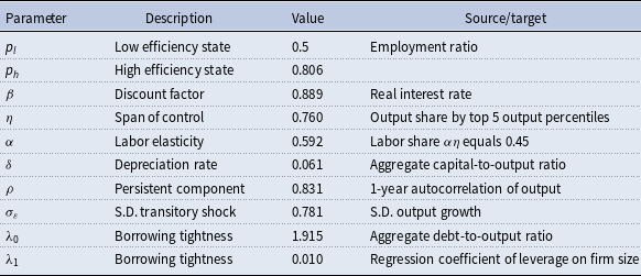
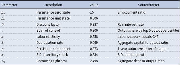
The model is annual. Parameters are calibrated to match the Chinese economy. Table 3 presents the calibration results for the model with the size-dependent borrowing constraint. This paper assumes that the idiosyncratic labor efficiency
 $v_{t}$
follows a two-state Markov process. The probability of low efficiency
 $p_{l}$
is set to 0.5, and the probability of high efficiency
 $p_{h}$
is equal to 0.806, so that the fraction of workers that supply labor in any given period is consistent with the employment ratio in China.Footnote
19
The rest of the parameters are jointly determined by adopting the simulated method of moments (SMM). The goal is to choose the set of parameters
 \begin{equation} \varTheta =\left \{ \beta,\eta,\delta,\rho,\sigma _{\varepsilon },\lambda _{0},\lambda _{1}\right \} \end{equation}
such that the distance between the moments generated by the model and moments from the Chinese data is minimized. The efficiency of the SMM requires the target moments to be sensitive to the variations in the structural parameters. Since each parameter affects more than one moment and some moments are more affected by certain parameters, the calibration procedures are as follows.
Calibration results
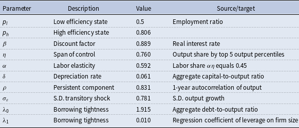
Note: This table reports the parameter values calibrated to match the empirical targets in the Chinese data, as discussed in the main text.
The discount factor
 $\beta$
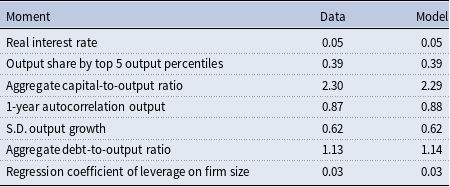
is set to match the real interest rate. I choose a targeted real interest rate of 5%, matching the average real interest rate of the USA during the sample period. As a result, the discount factor
 $\beta =0.889$
. As discussed in Buera et al. (Reference Buera, Kaboski and Shin2011), since in the data some of the payments to capital are actually payments to entrepreneurial input, it is difficult to obtain the capital share
 $(1-\alpha )\eta$
directly from the empirical work. To accommodate this difficulty, I first fix the labor share
 $\alpha \eta$
based on the existing literature and then calibrate the span of control
 $\eta$
. Bai and Qian (Reference Bai and Qian2010) estimate that the labor share in the Chinese industrial sector decreased from 0.49 in 1998 to 0.42 in 2004. In this paper, I set the labor share to 0.45. Given that the span of control
 $\eta$
affects the concentration of the output distribution,
 $\eta$
is calibrated to match the fraction of output by the top 5 output percentiles. As a result, the span of control
 $\eta =0.76$
. Then, the labor elasticity
 $\alpha$
is recovered as 0.592. The capital depreciation rate
 $\delta$
is set to match the aggregate capital-to-output ratio. The discount factor
 $\delta = 0.061$
, which is within the range of empirical evidence on capital depreciation in China.Footnote
20
The idiosyncratic productivity
 $z_{it}$
is assumed to follow an AR(1) process,
 \begin{equation} log(z_{it})=\rho log(z_{it-1})+\varepsilon _{it},\quad \varepsilon _{it}\sim N\!\left(0,\sigma _{\varepsilon }^{2}\right) \end{equation}
where
 $\rho$
is the persistent component,
 $\varepsilon _{it}$
stands for the transitory shock, and
 $\sigma _{\varepsilon }$
is the standard deviation of the transitory shock. Following the Rouwenhorst method (Reference Rouwenhorst and Rouwenhorst1995), I approximate this AR(1) process by a discrete Markov chain over a symmetric, evenly spaced state space. Considering that the productivity process is the primary determinant of the output, the moments that are used to identify the persistent component
 $\rho$
and the standard deviation of the transitory shock
 $\sigma _{\varepsilon }$
are (1) the first-order autocorrelation of the output, which is 0.87, and (2) the standard deviation of the output growth rate, which equals 0.62. The firm-level moments are based on the sample of Chinese non-SOEs for the period 1998-2007. As a result, the persistent component
 $\rho$
is 0.831, which is consistent with the existing literature. The standard deviation of the transitory shock
 $\sigma _{\varepsilon }=0.781$
, which is large to generate firm dynamics.
Parameters
 $\lambda _{0}$
and
 $\lambda _{1}$
jointly govern the borrowing tightness and determine firms’ financing patterns. In addition,
 $\lambda _{1}$
is primarily related to the leverage-size slope.Footnote
21
Thus, the moments used to pin down parameters
 $\lambda _{0}$
and
 $\lambda _{1}$
are (1) the regression coefficient of the leverage ratio on firm size, which is 0.03, and (2) the aggregate debt-to-output ratio.Footnote
22
Based on data from the World Bank, the average domestic credit to the private sector (% GDP) during the period 1998 to 2007 is 113%. As a result,
 $\lambda _{0}$
is 1.915, and
 $\lambda _{1}$
is 0.01. Under the size-dependent borrowing constraint, the implied maximum leverage ratio is
 $\left (d/k\right )_{max}=0.478+0.005k$
, which increases in capital.Footnote
23
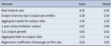
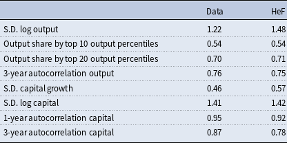
Table 4 reports the values of the target moments used to calibrate the parameters in the data and in the model. The model fits the data quite closely.
Model fit
Note: This table reports the empirical and model values of the moments used to calibrate the parameters. Moments are based on the sample of the Chinese non-SOEs for the period 1998-2007.
5. Quantitative results
This section studies the quantitative impacts of size-dependent financial frictions on capital misallocation and the aggregate TFP. I first evaluate the performance of the model with the size-dependent borrowing constraint (termed ”HeF” henceforth) and then examine the effects of the size-dependent financial frictions on capital misallocation. I also conduct a sensitivity analysis to examine the role of the borrowing tightness.
5.1. Model validation
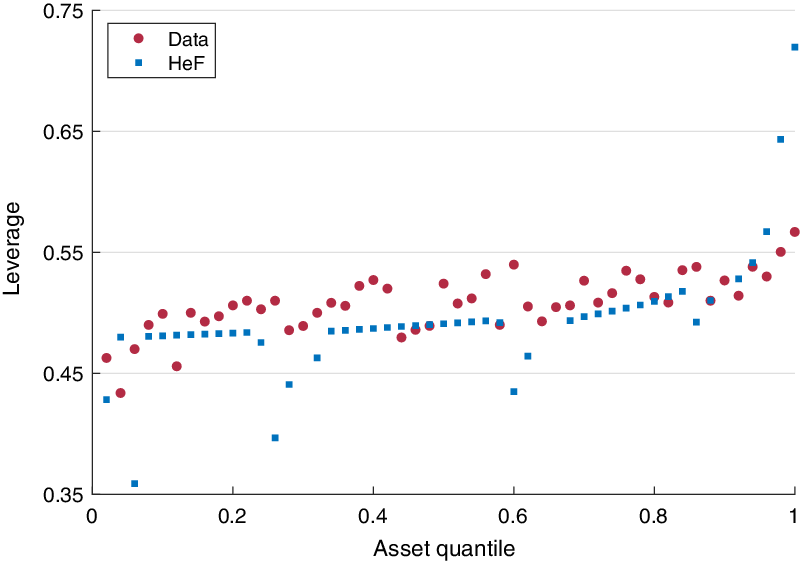
Financing behavior. To explore how well the HeF model with the size-dependent financial frictions matches the financing patterns of firms in the data, I first present the average leverage ratio conditional on asset quantiles. Figure 5 shows the relationship between leverage and firm size in the data and the model, respectively. As we can see, there is an increasing trend of leverage in both the model and the data, which suggests that large firms tend to have higher leverage.
Firm size and leverage in the data and HeF
Note: This figure reports the relationships between firm size and leverage in the model and in the data. The mean leverage ratio is calculated in each asset quantile (50 quantiles).

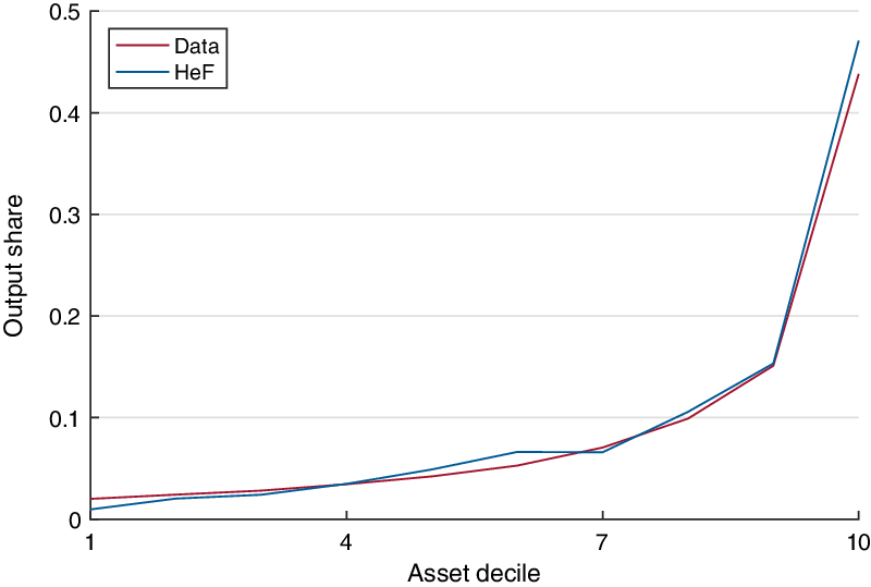
Output distribution. Figure 6 presents the output distribution by asset deciles in the data and in the model. The model reproduces the output distribution quite well. In the data, the top 10 and top 20 percentiles of firms by firm size account for 44% and 59% of the total output, and in the model, the top 10 and top 20 percentiles of firms contribute to 47% and 62% of the total output. The output distribution is highly skewed, and the output is concentrated in large firms.
Output distribution in the data and HeF
Note: This figure reports the output share by asset deciles in the model and in the data. The fraction of output of the total output is calculated in each asset decile.

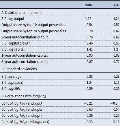
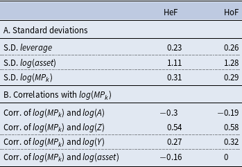
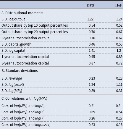
Non-targeted moments. Table 5 reports non-targeted moments in the data and the model with the size-dependent borrowing constraint, respectively. As shown in Panel A, the standard deviations of
 $log(Y)$
in the data (1.22) and model (1.24) are quite close. The model also matches the distribution of output by output quantiles, although I target only the output share of the top 5 output percentiles in the calibration. The model generates a larger standard deviation of capital growth, and the higher-order autocorrelations of capital and output in the model decay faster than those in the data.
Non-targeted firm-level moments in the data and HeF
Note: This table reports non-targeted moments in the data and model with the size-dependent borrowing constraint, respectively. Panel A presents the distributional moments of capital and output. Panel B reports the standard deviations of key variables. Panel C shows the correlations with marginal product of capital.
Panel B presents the standard deviations of leverage,
 $log(asset)$
and
 $log(MP_{k})$
. The standard deviation of leverage in both the model and data is 0.23. The standard deviation of total assets is 1.11, which is lower than the data. As discussed in Section 3, without distortions, the marginal product of capital across firms should be equal; the dispersion of the marginal product of capital endogenously arises in the model due to financial frictions. The standard deviation of
 $log(MP_{k})$
generated by the model is 0.31, which explains 35% of the dispersion of
 $log(MP_{k})$
in the data. The rationale for this result is that there are other forces in addition to financial frictions, such as taxes/subsidies, capital adjustment costs, and informational frictions, that contribute to capital misallocation.Footnote
24
The empirical work of Wu (Reference Wu2018) also suggests that significant capital misallocation in the Chinese manufacturing industry can be attributed to other policy distortions. Thus, this model, which focuses on financial frictions, does not generate a considerable dispersion of
 $log(MP_{k})$
.
The correlations with
 $log(MP_{k})$
show how the extent to which firms are distorted varies with firm characteristics. Since firms with higher net worth have stronger financing ability and are less likely to be constrained, they tend to face a lower marginal product of capital. Thus, the model with the size-dependent borrowing constraint generates a negative correlation between
 $log(MP_{k})$
and net worth
 $log(A)$
. Since firms with higher productivity tend to have a larger financing need and are more likely to be financially constrained, the model generates a positive correlation between
 $log(MP_{k})$
and productivity
 $log(Z)$
of 0.54. Moreover, since productivity is the primary determinant of output and firms with higher productivity tend to produce more, there is a positive correlation between
 $log(MP_{k})$
and
 $log(Y)$
. Furthermore, as large firms are less constrained under the size-dependent borrowing constraint, the correlation between
 $log(MP_{k})$
and firm size is −0.16, which is consistent with the data (−0.23). Overall, the model with the size-dependent borrowing constraint matches the firm-level moments of the Chinese manufacturing sector well.
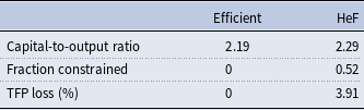
Aggregate Implications. Given the same amount of aggregate resources and the measure of producers as in the model, the planner allocates resources efficiently across firms. The marginal product of capital is equalized across firms in the efficient allocation. Table 6 reports the aggregate implications of both the efficient allocation and the model. The presence of financial frictions restrains capital allocation efficiency and aggregate output, as the aggregate capital-to-output ratio under financial frictions is higher than the first-best allocation with the same amount of aggregate capital. The fraction of firms that are financially constrained is 0.52, and the TFP loss in the model relative to the undistorted economy is 3.91%.
Aggregate implications in the HeF

Note: This table reports the aggregate implications of the efficient allocation and the model with the size-dependent borrowing constraint.
The TFP loss due to size-dependent financial frictions in the model is modest, which is mainly due to two factors. First, financial friction is one of the potential sources of capital misallocation. In addition, as discussed in Moll (Reference Moll2014), as long as productivity shocks are relatively persistent, self-financing alleviates capital misallocation in the long run. The productivity process in the model with the size-dependent borrowing constraint is persistent with the persistent component
 $\rho =0.83$
, which enables firms to accumulate enough internal funds in prolonged high-productivity periods and eliminate financial frictions. As a result, modest TFP loss is observed at the steady state.
5.2. The effect of size-dependent financial frictions
To examine the effect of size-dependent financial frictions on capital misallocation, I compare the baseline HeF model to the model with the homogeneous borrowing constraint in which
 $\lambda _{1}=0$
(termed “HoF”). I calibrate the borrowing tightness parameter
 $\lambda _{0}$
in the HoF model by targeting the aggregate credit to the private sector (% GDP). Appendix D.1 reports the calibration results and non-targeted moments. In the HoF model with the homogeneous borrowing constraint,
 $\lambda _{0}=2.498$
, which implies that the maximum attainable leverage ratioFootnote
25
for any firm is 0.6.Footnote
26
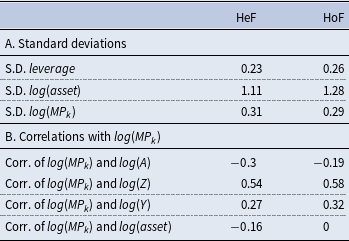
Non-targeted moments. Table 7 reports the non-targeted moments. The standard deviations of leverage and
 $log(MP_{k})$
in both models are quite close. A negative correlation between
 $log(MP_{k})$
and net worth
 $log(A)$
exists in both cases, since firms with higher net worth have stronger financing ability and are less likely to be affected by financial frictions. However, this negative correlation is stronger in the HeF (−0.3) than the HoF (−0.19), as some firms, even without sufficient net worth, are able to eliminate the borrowing constraint and face a low marginal product of capital in the HeF case. A positive correlation between
 $log(MP_{k})$
and
 $log(Z)$
also exists in the HoF case, since firms with higher productivity have a stronger financing need and are more likely to be constrained. However, since some highly productive firms in the HeF case will accumulate sufficient capital and relax the borrowing constraint, the HeF case generates a weaker correlation between
 $log(MP_{k})$
and
 $log(Z)$
(which is 0.54) than the HoF case (0.58). Accordingly, the HeF model with the size-dependent borrowing constraint generates a smaller correlation between
 $log(MP_{k})$
and
 $log(Y)$
than the HoF case.
Non-targeted firm-level moments in the HeF and HoF
Note: This table reports non-targeted moments in the HeF with the size-dependent borrowing constraint and the HoF with the homogeneous borrowing constraint. Panel A reports the standard deviations of key variables. Panel B shows the correlations with the marginal product of capital.
Firm size and capital misallocation. The critical difference between HeF and HoF lies in the correlation between firm size and
 $log(MP_{k})$
. As shown in Table 7, the HoF model without taking into account firms’ financing patterns fails to reproduce the correlation between firm size and
 $log(MP_{k})$
, as it equals zero. The correlation is -0.16 instead in the HeF case with the size-dependent borrowing constraint.
Both firm size and marginal product of capital depend on firms’ productivity and financing ability. When
 $\lambda _{1}=0$
with the homogeneous borrowing constraint, given productivity, firms with higher net worth tend to accumulate more capital and face a lower
 $MP_{k}$
; given net worth, firms with higher productivity tend to be larger and face a higher
 $MP_{k}$
. These two opposing forces shape the correlation between firm size and the marginal product of capital. Based on the calibration of the HoF model, the correlation between
 $log(MP_{k})$
and firm size is close to zero. By contrast, in the HeF model with positive
 $\lambda _{1}$
, some highly productive firms accumulate sufficient capital and relax the borrowing constraint. Therefore, the positive correlation between the marginal product of capital and productivity is weaker, and large firms face a lower
 $MP_{k}$
than in the case under the homogeneous borrowing constraint. This additional channel making large firms less distorted by financial frictions accounts for the negative correlation between firm size and
 $log(MP_{k})$
in the HeF case.
To further study the pattern of
 $log(MP_{k})$
across different size groups, I compute and compare the mean and standard deviation of
 $log(MP_{k})$
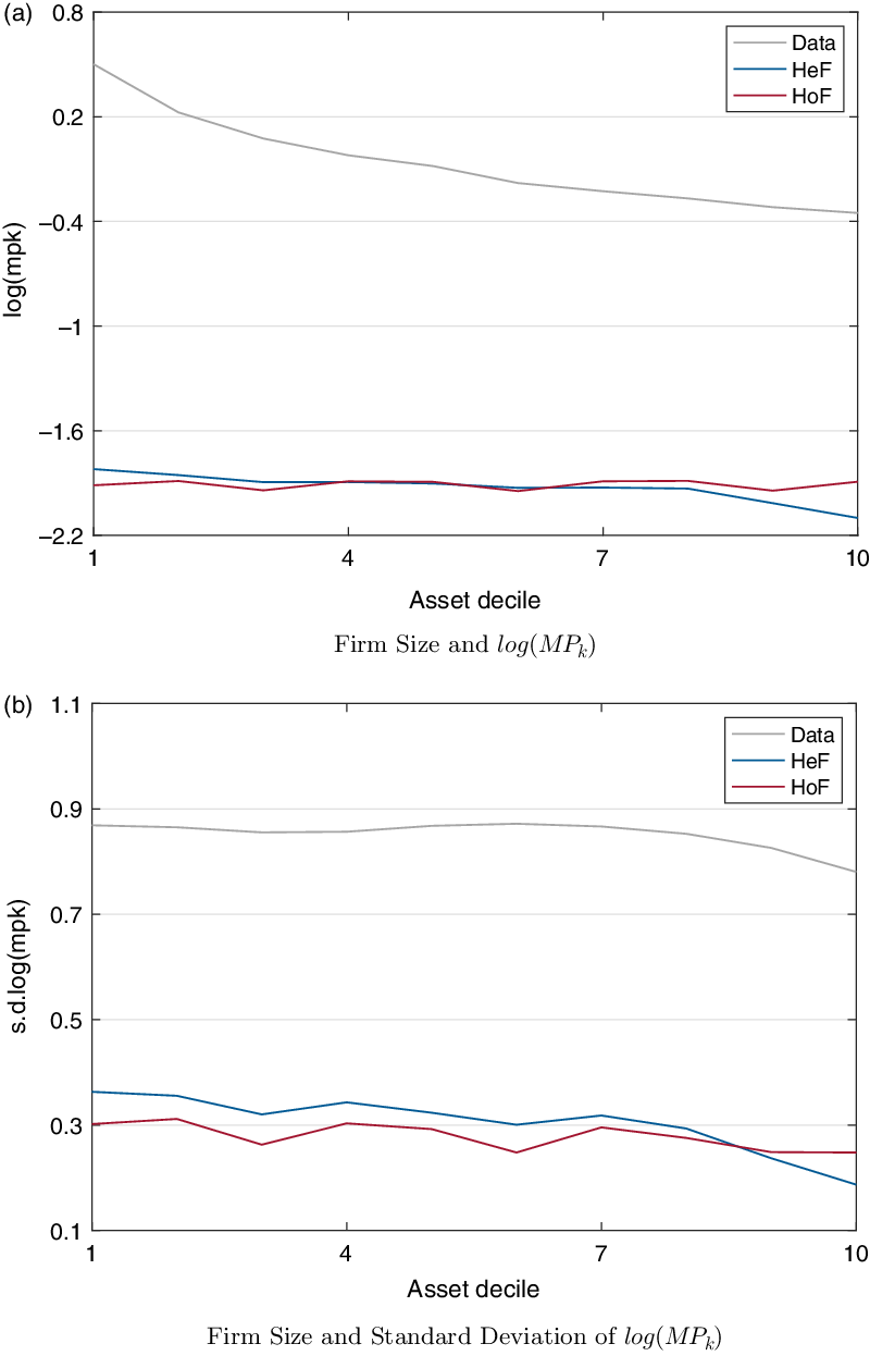
conditional on asset deciles. Figure 7 panel (a) reports the relationship between firm size and
 $log(MP_{k})$
. In HeF under the size-dependent borrowing constraint,
 $log(MP_{k})$
decreases with firm size. In HoF under the homogeneous borrowing constraint,
 $log(MP_{k})$
fluctuates slightly and does not demonstrate a downward trend. Moreover, the mean of
 $log(MP_{k})$
among large firms (top 20% by assets) is lower in HeF than in HoF. The standard deviations of
 $log(MP_{k})$
in the two models also vary across different size groups. As shown in Figure 7 panel (b), with the size-dependent borrowing constraint, the standard deviation of
 $log(MP_{k})$
decreases from 0.37 to 0.18 as firm size increases. The dispersion of
 $log(MP_{k})$
among large firms (top 20% by assets) is also smaller in HeF than in HoF.
Firm size and
 $log(MP_{k})$
in the HeF and HoF
Note: This figure reports the relationships between firm size and
 $log(MP_{k})$
in the HeF with the size-dependent borrowing constraint and the HoF with the homogeneous borrowing constraint. The mean and standard deviation of
 $log(MP_{k})$
are calculated in each asset decile.

Although the model with the size-dependent borrowing constraint is able to reproduce the patterns of the marginal product of capital by firm size, they are more muted than in the data. In panel (a), the downward trend of
 $log(MP_{k})$
in HeF is fatter than in the data, implying that other factors may also contribute to the negative relationship. The standard deviation of
 $log(MP_{k})$
in HeF is also smaller than in the data, suggesting the existence of other distortions in addition to financial frictions resulting in misallocation. As discussed in David and Venkateswaran (Reference David and Venkateswaran2019), adjustment and information frictions account for relatively modest fractions of the misallocation among Chinese firms, and the predominant drivers lie in firm-specific factors, especially the size/productivity-dependent policies. Therefore, other factors, for example, adjustment and information frictions, and firm-specific distortions, in addition to size-dependent financial frictions, may explain the gap in the marginal product of capital between the HeF case and data.
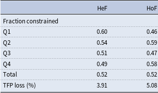
Aggregate implications. Table 8 reports the aggregate implications. As shown in the 7th row, the fractions of firms that are financially constrained at steady state in the two models are quite close. The fraction of firms that are constrained in each asset quartile is computed and compared (rows 3-6). In the HeF model, 60% of firms in the first asset quartile are constrained, which decreases to 49% in the fourth quartile. Large firms (the fourth asset quartile) are less likely to be financially constrained in HeF than in HoF.
Aggregate implications in the HeF and HoF

Note: This table reports the aggregate implications in the HeF with the size-dependent borrowing constraint and the HoF with the homogeneous borrowing constraint. The fraction of firms that are constrained is calculated in each asset quartile (Q1-Q4).
Firm-level moments in the sensitivity analysis

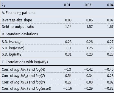
Note: This table reports the firm-level moments in the baseline HeF model with
 $\lambda _{1}=0.01$
and for
 $\lambda _{1}=0.03$
and
 $\lambda _{1}=0.04$
. Panel A reports financing patterns. Panel B presents the standard deviations of key variables. Panel C shows the correlations with the marginal product of capital.
Table 8 also shows the TFP loss in the two models. Whether firms’ financing pattern (the positive leverage-size slope) is considered affects the measured TFP loss. The TFP loss in the HeF model is 3.91%, which is smaller than in the HoF case (5.08%).Footnote
27
As discussed above, in the HeF model with the size-dependent borrowing constraint, some highly productive firms accumulate sufficient capital and eliminate the borrowing constraint. Thus, the marginal product of capital is less correlated with productivity than in the HoF case. Since large (or highly productive) firms, which contribute to the majority of output, are actually less distorted by financial frictions with both a lower mean and standard deviation of
 $log(MP_{k})$
, the model generates a smaller TFP loss under the size-dependent financial frictions than in the HoF case.
Overall, the model with a size-dependent borrowing constraint is more suitable for matching the Chinese firm-level moments than the alternative. The model predicts a negative correlation between firm size and the marginal product of capital, which is a feature lacking in the HoF model with the homogenous borrowing constraint. In addition, the model generates both a lower mean and standard deviation of the marginal product of capital among large firms than the HoF model. Without considering the size-dependent financial policy, the TFP loss may be overestimated, since large firms, which contribute the most to the economy, are more leveraged and less distorted by financial frictions.
5.3. Sensitivity analysis
Since under the size-dependent borrowing constraint, the borrowing tightness parameter
 $\lambda _{1}$
plays an essential role in the firm’s financing patterns, this subsection examines the impacts of
 $\lambda _{1}$
on capital misallocation. Table 9 reports the moments in terms of financing pattern and capital misallocation. Column 2 presents the moments in the baseline HeF model with
 $\lambda _{1}=0.01$
, and columns 3-4 report the corresponding moments as
 $\lambda _{1}$
increases. When
 $\lambda _{1}= 0.03$
, the maximum attainable leverage ratio
 $\left (d/k\right )_{max}=0.478+0.016k$
, and when
 $\lambda _{1}= 0.04$
,
 $\left (d/k\right )_{max}=0.478+0.021k$
. As shown in Table 9, when
 $\lambda _{1}$
increases, the leverage-size slope increases accordingly, since large firms are more favored in the financial market. As the increasing
 $\lambda _{1}$
also implies a decreasing borrowing tightness, the aggregate debt-to-output ratio increases, leverage and
 $log(asset)$
become more volatile with the higher standard deviations, and the dispersion of
 $log(MP_{k})$
decreases consequently.
The changes in financing patterns affect capital misallocation accordingly. As
 $\lambda _{1}$
increases, firms without high net worth are more likely to eliminate the borrowing constraint than before. As a result, the negative correlation between net worth and
 $log(MP_{k})$
becomes stronger. Firms with high productivity are less likely to be constrained than previously, and thus, the positive correlation between productivity and
 $log(MP_{k})$
weakens. As large firms are even more favored in the financial market, the negative correlation between firm size and
 $log(MP_{k})$
becomes stronger.
Although as
 $\lambda _{1}$
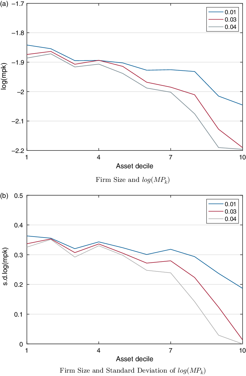
increases, the maximum attainable leverage ratio for all firms increases compared with the baseline HeF model, large firms benefit more from the increasing leverage-size slope than small firms. Figure 8 presents the mean and standard deviation of
 $log(MP_{k})$
conditional on asset deciles in the baseline HeF model with
 $\lambda _{1}=0.01$
and when
 $\lambda _{1}=0.03$
and
 $\lambda _{1}=0.04$
. As we can see from panels (a) and (b), as
 $\lambda _{1}$
increases, the average and standard deviation of
 $log(MP_{k})$
decrease. Moreover, both the mean and dispersion of
 $log(MP_{k})$
decrease further among large firms.
Firm size and
 $log(MP_{k})$
in the sensitivity analysis
Note: This figure reports the relationship between firm size and
 $log(MP_{k})$
in the baseline HeF model with
 $\lambda _{1}=0.01$
and when
 $\lambda _{1}=0.03$
and
 $\lambda _{1}=0.04$
, respectively. The mean and standard deviation of
 $log(MP_{k})$
are calculated in each asset decile.

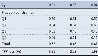
Table 10 reports the aggregate implications. As
 $\lambda _{1}$
increases, the fraction of firms that are constrained becomes smaller accordingly. In addition, the fraction constrained decreases more among large firms. When
 $\lambda _{1}$
increases from 0.01 to 0.03, the fraction constrained in the fourth asset quartile decreases from 0.49 to 0.21 (decreased by 57%), and when
 $\lambda _{1}=0.04$
, only 12% of the firms are constrained in that size group. The TFP loss decreases accordingly, as firms, especially large firms, are less financially constrained when the leverage-size slope increases.
Aggregate implications in the sensitivity analysis

Note: This table reports the aggregate implications in the baseline HeF model with
 $\lambda _{1}=0.01$
and when
 $\lambda _{1}=0.03$
and
 $\lambda _{1}=0.04$
, respectively. The fraction of firms that are constrained is calculated in each asset quartile (Q1-Q4).
6. Conclusion
This paper studies the impacts of financial frictions on capital misallocation and aggregate productivity based on the Chinese manufacturing dataset. To capture the empirical feature that large firms have a higher leverage ratio than small firms, this paper formulates a general equilibrium model of firm dynamics based on Midrigan and Xu (Reference Midrigan and Xu2014) and introduces size-dependent financial frictions in light of Gopinath et al. (Reference Gopinath, Kalemli-Özcan, Karabarbounis and Villegas-Sanchez2017). With the size-dependent borrowing constraint, the borrowing tightness decreases with firm size. I calibrate the model using the Chinese firm-level dataset to identify the productivity process and borrowing tightness parameters. Under the size-dependent borrowing constraint, since larger firms are less likely to be distorted by financial frictions, this paper predicts a negative correlation between firm size and the marginal product of capital, which is a feature that the model with a homogeneous borrowing constraint fails to capture. The model with a size-dependent borrowing constraint predicts a TFP loss of 3.91%, which is modest and can be rationalized by firms’ self-financing. Moreover, the TFP loss may be overstated without considering the size-dependent financial policy, since large firms are actually less distorted by financial frictions.
This paper can be extended in several directions. For example, since the fixed costs of entry and technology adoption are nontrivial, financial frictions may play a more substantial role along the extensive margin by distorting firms’ entry and technology adoption decisions than on the intensive margin through capital misallocation. In addition, this paper studies resource misallocation among non-SOEs in the Chinese manufacturing sector. In the future, I will investigate the impacts of cross-sector resource misallocation on aggregate productivity.
Appendices
A. Data
A.1. Data cleaning
This paper focuses on the firm-level dataset from the Chinese Annual Survey of Industrial Firms, which is published by the National Bureau of Statistics (NBS) of China. This dataset includes all state-owned firms and all “above-scale” non-state-owned firms with annual sales exceeding 5 million RMB. This dataset covers the industries of manufacturing, mining, and public utilities and includes a wealth of firm-level information, such as firms’ balance sheets, output, and revenues. The sample period is from 1998 to 2007. The steps of the data cleaning process are as follows.
Dropping invalid observations. First, observations with negative key variables are deleted. I drop observations with a negative industrial value added, employment, fixed assets at the original price, total assets, and total liabilities. Next, I drop observations that violate the accounting standards required by the China Industrial Statistics Reporting System because (1) the fixed asset at the original price is smaller than the accumulated depreciation; (2) the fixed asset at the original price is smaller than the net fixed asset; (3) the accumulated depreciation is smaller than the current depreciation; (4) the total assets are smaller than the sum of current assets, long-term investments, fixed assets, and intangible assets; (5) the total debt is smaller than the sum of short-term and long-term debt; (6) the industrial output is smaller than the industrial value added or smaller than the intermediate input. Furthermore, I restrict the sample within the manufacturing sector.
Industry classification. Since there was a change in the China Industry Classification (CIC) system starting in 2003, another task when dealing with this dataset is to unify the industry classification over the years. Following the method of Brandt et al. (Reference Brandt, Van Biesebroeck and Zhang2014), this paper adopts a revision of the CIC system of manufacturing with 593 four-digit industries and 30 two-digit industries. Each firm is classified into one particular industry.
Firm ID. Another challenge when dealing with this dataset is that although the firm ID information is reported in the original dataset, there is no unique firm ID to identify the same firm that exists in multiple years. For example, a firm may be assigned to different IDs over the years due to a change in the firm name. Following Brandt et al. (Reference Brandt, Van Biesebroeck and Zhang2014), this paper identifies the same firms by combining information on the firm ID, legal identity, region, phone number, industry, founding year, product, and then assigns a unique ID to each firm in this dataset.
Firm ownership. Considering that in China, SOEs have easier access than non-SOEs to external finance, this paper divides firms into SOEs and non-SOEs according to their ownership. According to the Chinese Annual Survey of Industrial Firms, two indicators help identify ownership: (1) registered ownership and (2) registered capital. One problem of using registered ownership is that in China, actual ownership may not be consistent with registered ownership. For example, if the ratio of Hong Kong, Macau, Taiwan (HMT) or foreign capital to total registered capital is larger than 25%, then the firm can be legally registered as a non-SOE, even though this firm is actually controlled by the state. Thus, following Wu (Reference Wu2018) and Hsieh and Song (Reference Hsieh and Song2015), this paper identifies firm ownership by using registered capital. As long as the ratio of state capital to total registered capital is no less than 50%, the firm is identified as an SOE. Otherwise, the firm is a non-SOE.
A.2. Variable definition
This part describes the definitions and measures of the variables.
Output. The output is measured by the value added, which is directly reported in the dataset, and is then deflated by the GDP deflator.
Capital stock. There is a lack of a good measure of capital stock in the dataset. Following Brandt et al. (Reference Brandt, Van Biesebroeck and Zhang2014), the real capital stock series is constructed by adopting the perpetual inventory method.
Labor. There are two measures of labor: (1) employment and (2) wage and welfare compensation. To control the differences in the quality of labor within and across firms, following Gopinath et al. (Reference Gopinath, Kalemli-Özcan, Karabarbounis and Villegas-Sanchez2017), this paper uses the sum of wages and welfare payments as the measure of labor.
Total assets. Total assets are defined as the sum of current assets, long-term investments, fixed assets, and intangible assets. This variable is directly reported in the dataset.
Total debt. Total debt is the sum of long-term and short-term debt. This variable is directly reported in the dataset.
Leverage. Leverage is defined as the ratio of total debt to total assets. In this paper, leverage is restricted within the range of
 $[0,1]$
.
B. Derivations and proofs
B.1. Microfoundation of the size-dependent borrowing constraint
The paper extends the underlying logic of the borrowing constraint in the existing literature motived by limited commitment (e.g. Moll, Reference Moll2014; Buera and Moll, Reference Buera and Moll2015; Midrigan and Xu, Reference Midrigan and Xu2014). Suppose that contract enforcement is limited and default risks exist. If the firm redeems its debt, the firm solves the problem
 \begin{equation} V^{N}(k,d,z)=\max _{k^{\prime},d^{\prime},c}log(c)+\beta EV(k^{\prime},d^{\prime},z^{\prime}) \end{equation}
subject to the budget constraint
 \begin{equation} c_{it}+k_{it+1}-(1-\delta )k_{it}=y_{it}-W l_{it}-(1+r)d_{it}+d_{it+1} \end{equation}
In case of default, the firm defaults on a fraction
 $\mu _{0}$
of its debt
 $d_{it}$
. As a penalty, the bank seizes a fraction
 $\mu _{1}$
of the undepreciated capital
 $(1-\delta )k_{it}$
. There is a disruption cost in the event of default that the firm has to pay
 $\Phi (k_{it})$
, following Gopinath et al. (Reference Gopinath, Kalemli-Özcan, Karabarbounis and Villegas-Sanchez2017). Other default benefits are summarized in the term
 $\mu _{3}k_{it}$
. In addition, we assume that firms that default still have access to the financial market in the next period for simplification. Thus, the firm solves the problem
 \begin{equation} V^{D}(k,d,z)=\max _{k^{\prime},d^{\prime},c}log(c)+\beta EV(k^{\prime},d^{\prime},z^{\prime}) \end{equation}
subject to the budget constraint
 \begin{equation} c_{it}+k_{it+1}-(1-\delta )k_{it}=y_{it}-W l_{it}-(1+r-\mu _{0})d_{it}-\mu _{1}(1-\delta )k_{it}-\mu _{2}\Phi (k_{it})+\mu _{3}k_{it}+d_{it+1} \end{equation}
The firm chooses not to default if and only if
 \begin{equation} V^{N} \geq V^{D} \end{equation}
Therefore, we can obtain the incentive compatibility constraint so that there is no default in the equilibrium as follows:
 \begin{equation} d_{it}\leq \underbrace{\left (\frac{\mu _{1}\!\left (1-\delta \right )-\mu _{3}}{\mu _{0}}\right )}_{\theta _{0}}k_{it}+\underbrace{\left (\frac{\mu _{2}}{\mu _{0}}\right )}_{\theta _{1}}\!\Phi (k_{it}) \end{equation}
Define net worth
 $a_{it}=k_{it}-d_{it}\geq 0$
. Thus, the borrowing constraint can be rewritten as
 \begin{equation} k_{it}\leq \underbrace{\left (\frac{\mu _{0}}{\mu _{0}-\mu _{1}\!\left (1-\delta \right )+\mu _{3}}\right )}_{\lambda _{0}}a_{it}+\underbrace{\left (\frac{\mu _{2}}{\mu _{0}-\mu _{2}\!\left (1-\delta \right )+\mu _{3}}\right )}_{\lambda _{1}}\!\Phi (k_{it}) \end{equation}
where
 $\lambda _{0}=\frac{1}{1-\theta _{0}}$
and
 $\lambda _{1}=\frac{\theta _{1}}{1-\theta _{0}}$
.
B.2. Parameter restrictions on the size-dependent borrowing constraint
Parameter restrictions are imposed to ensure that defaulting is costly. The default cost is
 \begin{equation} \begin{array}{ll} C(k) &= \mu _{1}(1-\delta )k+\mu _{2}\Phi (k)-\mu _{3}k\\ &= \left (\mu _{1}\!(1-\delta )-\mu _{3}\right )\!k+\mu _{2}k^{2} \end{array} \end{equation}
As long as
 $\mu _{1}\!\left (1-\delta \right )-\mu _{3}\geq 0$
,
 $C(k)\geq 0$
. To ensure that both
 $\lambda _{0}$
and
 $\lambda _{1}$
are nonnegative, another appropriate restriction is
 $\mu _{0}-\mu _{1}\!\left (1-\delta \right )+\mu _{3}\geq 0$
. Based on the expressions for
 $\lambda _{0}$
and
 $\lambda _{1}$
in Appendix B.1, the resulting parameter restrictions are
 $\lambda _{0}\geq 1$
and
 $\lambda _{1}\geq 0$
.
If
 $\mu _{2}=0$
, then
 $\theta _{1}=0$
, and
 $\lambda _{1}=0$
. In this case, the size-dependent financial friction channel is closed.
B.3. Proof of proposition 1
Proof. Under the size-dependent borrowing constraint,
 $FOCs$
with respect to labor
 $l$
and capital
 $k$
are given by
 \begin{equation} \alpha \eta \frac{y(a,z)}{l(a,z)}=W \end{equation}
 \begin{equation} \left (1-\alpha \right )\!\eta \frac{y(a,z)}{k(a,z)}=r+\delta +\mu (a,z)\!\left [1-2\lambda _{1}k(a,z)\right ] \end{equation}
where
 $\mu (a,z)$
is the Lagrangian multiplier on the borrowing constraint:
 \begin{equation} \mu (a,z)=\begin{cases} 0 & if\;k(a,z)\lt \lambda _{0}a+\lambda _{1}k(a,z)^{2}\\[5pt]
\frac{1}{(1-2\lambda _{1}k(a,z))}\left[\left (\frac{\alpha \eta }{W}\right )^{\frac{\alpha \eta }{1-\eta }}\!\left (1-\alpha \right )\eta\!\left (\frac{z}{k(a,z)}\right )^{\frac{1-\eta }{1-\alpha \eta }}-r-\delta \right] & if\;k(a,z)=\lambda _{0}a+\lambda _{1}k(a,z)^{2} \end{cases} \end{equation}
Then,
 $l$
and
 $k$
can be jointly solved as
 \begin{equation} l(a,z)=z^{\frac{1-\eta }{1-\alpha \eta }}\!\left(\frac{\alpha \eta }{W}\right)^{\frac{1}{1-\alpha \eta }}k{}^{\frac{(1-\alpha )\eta }{1-\alpha \eta }} \end{equation}
 \begin{equation} k(a,z)=z\!\left(\frac{\alpha \eta }{W}\right)^{\frac{\alpha \eta }{1-\eta }}\!((1-\alpha )\eta )^{\frac{1-\alpha \eta }{1-\eta }}\left[r+\delta +\mu (a,z)(1-2\lambda _{1}k(a,z))\right]^{\frac{\alpha \eta -1}{1-\eta }} \end{equation}
To obtain a closed-form solution for capital, I define the function
 $g(k)$
as the difference between the
 $RHS$
and
 $LHS$
of the borrowing constraint:
 \begin{equation} g(k)\equiv \lambda _{0}a+\lambda _{1}k^{2}-k \end{equation}
When the borrowing constraint is slack, the capital decision
 $k^{u}$
is
 \begin{equation} k^{u}=\left(\frac{\alpha \eta }{W}\right)^{\frac{\alpha \eta }{1-\eta }}\left(\frac{(1-\alpha )\eta }{r+\delta }\right)^{\frac{1-\alpha \eta }{1-\eta }}z \end{equation}
which satisfies both
 $\mu =0$
and
 $g(k)\gt 0$
. In this case,
 $k^{u}$
increases in productivity
 $z$
.
When the borrowing constraint is binding,
 $g(k)=0$
. As long as
 $1-4\lambda _{0}\lambda _{1}a\geq 0$
, there are two real roots
 $k_{1}$
and
 $k_{2}$
for
 $g(k)=0$
(where
 $k_{1}\leq k_{2}$
). Figure B.1 presents the curve for
 $g(k)$
when
 $g(k)=0$
has two real roots. Since when
 $k=\frac{1}{2\lambda _{1}}$
,
 $g(k)$
achieves its minimum value, the relative relationship between
 $k_{1}$
and
 $k_{2}$
is
 \begin{equation} 0\leq k_{1}\leq \frac{1}{2\lambda _{1}}\leq k_{2} \end{equation}
Only when capital
 $k^{c}=k_{1}$
are both
 $\mu \gt 0$
and
 $g(k)=0$
satisfied. Thus, firms that face a binding borrowing constraint can achieve a capital level of only
 $k^{c}(a,z)$
, which is the smaller root
 $k_{1}$
of
 $g(k)=0$
:
 \begin{equation} k^{c}(a,z)=\frac{1-\sqrt{1-4\lambda _{0}\lambda _{1}a}}{2\lambda _{1}} \end{equation}
Graph for function
 $g(k)$
Note: This figure presents the graph for
 $g(k)$
. The number of intersections with the horizontal axis depends on borrowing tightness parameters
 $\lambda _{0}$
and
 $\lambda _{1}$
, and net worth
 $a$
.

B.4. Proof of proposition 2
Proof. When
 $\lambda _{1}=0$
, the borrowing constraint is
 \begin{equation} k\leq \lambda _{0}a \end{equation}
The
 $FOCs$
with respect to labor
 $l$
and capital
 $k$
are
 \begin{equation} \alpha \eta \frac{y(a,z)}{l(a,z)}=W \end{equation}
 \begin{equation} \left (1-\alpha \right )\eta \frac{y(a,z)}{k(a,z)}=r+\delta +\gamma (a,z) \end{equation}
where
 $\gamma (a,z)$
is the Lagrangian multiplier on the borrowing constraint given by
 \begin{equation} \gamma (a,z)=\begin{cases} 0 & if\;k(a,z)\lt \lambda _{0}a\\ \left (\frac{\alpha \eta }{W}\right )^{\frac{\alpha \eta }{1-\eta }}\!\left (1-\alpha \right )\eta\! \left (\frac{z}{k(a,z)}\right )^{\frac{1-\eta }{1-\alpha \eta }}-r-\delta & if\;k(a,z)=\lambda _{0}a \end{cases} \end{equation}
Then,
 $l$
and
 $k$
can be jointly solved as
 \begin{equation} l(a,z)=z^{\frac{1-\eta }{1-\alpha \eta }}\!\left(\frac{\alpha \eta }{W}\right)^{\frac{1}{1-\alpha \eta }}\!k{}^{\frac{(1-\alpha )\eta }{1-\alpha \eta }} \end{equation}
 \begin{equation} k(a,z)=z\left(\frac{\alpha \eta }{W}\right)^{\frac{\alpha \eta }{1-\eta }}((1-\alpha )\eta )^{\frac{1-\alpha \eta }{1-\eta }}[r+\delta +\gamma (a,z)]^{\frac{\alpha \eta -1}{1-\eta }} \end{equation}
When the borrowing constraint is slack, the capital decision
 $k^{u}$
is
 \begin{equation} k^{u}=\left(\frac{\alpha \eta }{W}\right)^{\frac{\alpha \eta }{1-\eta }}\!\left(\frac{(1-\alpha )\eta }{r+\delta }\right)^{\frac{1-\alpha \eta }{1-\eta }}z \end{equation}
In this case, capital
 $k^{u}$
increases in productivity
 $z$
.
When the borrowing constraint is binding, the attainable capital level
 $k^{c}$
is
 \begin{equation} k^{c}=\lambda _{0}a \end{equation}
In this case,
 $k^{c}$
is linear in net worth
 $a$
.
Given a productivity
 $z$
, when the borrowing constraint is exactly binding,
 $k^{u}=k^{c}$
. Then, the cutoff net worth
 $a^{*}$
is
 \begin{equation} a^{*}=\frac{k^{u}(z)}{\lambda _{0}} \end{equation}
If
 $a\leq{a^{*}}$
, the borrowing constraint is binding. If
 $a\gt a^{*}$
, the borrowing constraint is slack. When the net worth
 $a$
is large enough, for example,
 $a\gt \frac{k^{u}(\bar{z})}{\lambda _{0}}$
, the borrowing constraint is never binding.
B.5. Proof of proposition 3
Proof. Under the size-dependent borrowing constraint (
 $\lambda _{1}\gt 0$
), according to Proposition 1,
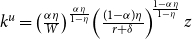 $k^{u}=\left(\frac{\alpha \eta }{W}\right)^{\frac{\alpha \eta }{1-\eta }}\!\left(\frac{(1-\alpha )\eta }{r+\delta }\right)^{\!\frac{1-\alpha \eta }{1-\eta }}z$
, and
 $k^{c}(a)=\frac{1-\sqrt{1-4\lambda _{0}\lambda _{1}a}}{2\lambda _{1}}$
. Given productivity
 $z$
, when the borrowing constraint is exactly binding,
 $k^{u}=k^{c}$
. Then, the cutoff net worth
 $a^{*}$
is
 \begin{equation} a^{*}=\frac{1-\left (1-2\lambda _{1}k^{u}(z)\right )^{2}}{4\lambda _{0}\lambda _{1}} \end{equation}
If
 $a\leq{a^{*}}$
, the borrowing constraint is binding. If
 $a\gt a^{*}$
, the borrowing constraint is slack. When the net worth
 $a$
is large enough, for example,
 $a\gt \frac{1}{4\lambda _{0}\lambda _{1}}$
, the borrowing constraint is never binding.
B.6. Proof of proposition 4
Proof. Based on Appendix B.4, the marginal product of capital
 $MP_{k}$
under the homogeneous borrowing constraint is equal to
 \begin{equation} MP_{k}=r+\delta +\gamma \end{equation}
The capital decisions for the financially unconstrained and constrained firms are
 $k^{u}=\left(\frac{\alpha \eta }{W}\right)^{\frac{\alpha \eta }{1-\eta }}\left(\frac{(1-\alpha )\eta }{r+\delta }\right)^{\frac{1-\alpha \eta }{1-\eta }}z$
and
 $k^{c}(a)=\lambda _{0}a$
, respectively. Let
 $a^{*}=\frac{k^{u}(z)}{\lambda _{0}}$
,
 $a_{1}=\frac{k^{u}(\underline{z})}{{{\lambda _{0}}}}$
,
 $a_{2}=\frac{k^{u}(\bar{z})}{{{\lambda _{0}}}}$
,
 $c=\left(\frac{\alpha \eta }{W}\right)^{\frac{\alpha \eta }{1-\eta }}((1-\alpha )\eta )^{\frac{1-\alpha \eta }{1-\eta }}(r+\delta )^{\frac{\alpha \eta -1}{1-\eta }}$
, and
 $z^{*}=\frac{k^{c}(a)}{c}$
, where
 $z^{*}$
is the cutoff productivity for bindingness given
 $a$
. Then, the relationship between the net worth
 $a$
, productivity
 $z$
, capital
 $k$
, and marginal product of capital
 $MP_{k}$
is the following:
-
1. Given a productivity
$z$
:
-
(1) firms are constrained, as
$a\in \left [\underline{a}, a^{*}\right ]$
. Firms with a larger net worth
$a$
have higher capital
$k^{c}(a)$
and lower
$\gamma$
and
$MP_{k}$
; -
(2) firms are unconstrained, as
$a\in (a^{*}, \bar{a}]$
. The capital
$k^{u}(z)$
is constant; in addition,
$\gamma =0$
, and
$MP_{k}=r+\delta$
.
-
-
2. Given a net worth
$a$
:
-
(1) when
$a\in \left [\underline{a},a_{1}\right ]$
, firms are constrained, as
$z\in [\underline{z},\bar{z}]$
. Firms with higher productivity
$z$
have higher
$\gamma$
and
$MP_{k}$
, as capital
$k^{c}(a)$
does not change; -
(2) when
$a\in (a_{1},a_{2}]$
, 1) firms are unconstrained, as
$z\in [\underline{z}, z^{*})$
. Firms with higher productivity
$z$
have higher
$k^{u}(z)$
; in addition,
$\gamma =0$
, and
$MP_{k}=r+\delta$
; 2) firms are constrained, as
$z\in \left [z^{*}, \bar{z}\right ]$
. Firms with higher productivity
$z$
have higher
$\gamma$
and
$MP_{k}$
, as the capital
$k^{c}(a)$
does not change; -
(3) when
$a\in (a_{2},\bar{a}]$
, firms are unconstrained, as
$z\in [\underline{z},\bar{z}]$
. Firms with higher productivity
$z$
have higher
$k^{u}(z)$
; in addition,
$\gamma =0$
, and
$MP_{k}=r+\delta$
.
-


Figure B.2 reports the relationships between net worth
 $a$
, productivity
 $z$
, and
 $MP_{k}$
under the homogeneous borrowing constraint. The idiosyncratic productivity is discretized into nine equally spaced states, and a brighter color corresponds to a higher
 $MP_{k}$
. Given a productivity shock
 $z,$
firms with a higher net worth
 $a$
tend to face a lower
 $MP_{k}$
, since the higher net worth helps relax the borrowing constraint. In addition, given a net worth
 $a$
, the marginal product of capital
 $MP_{k}$
increases fully with increasing productivity. That is, firms with higher productivity accordingly have a higher financing need for capital. As a result, those firms are more constrained and face a higher
 $MP_{k}$
.
Determination of the marginal product of capital (
 $\lambda _{1}=0$
)
Note: This figure reports the relationship between the state
 $(a,z)$
and the marginal product of capital
 $MP_{k}$
under the homogeneous borrowing constraint.

B.7. Proof of proposition 5
Proof. The marginal product of capital
 $MP_{k}$
under the size-dependent borrowing constraint is equal to
 \begin{equation} MP_{k}=r+\delta +\mu (1-2\lambda _{1}k) \end{equation}
According to Proposition 1,
 $k^{u}=\left(\frac{\alpha \eta }{W}\right)^{\frac{\alpha \eta }{1-\eta }}\left(\frac{(1-\alpha )\eta }{r+\delta }\right)^{\frac{1-\alpha \eta }{1-\eta }}z$
,
 $k^{c}(a)=k_{1}(a)=\frac{1-\sqrt{1-4\lambda _{0}\lambda _{1}a}}{2\lambda _{1}}$
, and
 $k_{2}(a)=\frac{1+\sqrt{1-4\lambda _{0}\lambda _{1}a}}{2\lambda _{1}}$
. Let
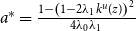 $a^{*}=\frac{1-\left (1-2\lambda _{1}k^{u}(z)\right )^{2}}{4\lambda _{0}\lambda _{1}}$
,
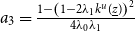 $a_{3}=\frac{1-\left (1-2\lambda _{1}k^{u}(\underline{z})\right )^{2}}{4\lambda _{0}\lambda _{1}}$
,
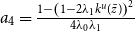 $a_{4}=\frac{1-\left (1-2\lambda _{1}k^{u}(\bar{z})\right )^{2}}{4\lambda _{0}\lambda _{1}}$
,
 $a_{5}=\frac{1}{4\lambda _{0}\lambda _{1}}$
,
 $c=(\frac{\alpha \eta }{W})^{\frac{\alpha \eta }{1-\eta }}((1-\alpha )\eta )^{\frac{1-\alpha \eta }{1-\eta }}(r+\delta )^{\frac{\alpha \eta -1}{1-\eta }}$
,
 $z^{*}_{1}=\frac{k_{1}(a)}{c}$
, and
 $z^{*}_{2}=\frac{k_{2}(a)}{c}$
, where
 $z^{*}_{1}$
and
 $z^{*}_{2}$
are the cutoff productivities for bindingness given
 $a$
. The relationship among the net worth
 $a$
, productivity
 $z$
, capital
 $k$
, and marginal product of capital
 $MP_{k}$
under the size-dependent borrowing constraint is as follows:
-
1. Given a productivity
$z$
:
-
(1) firms are constrained, as
$a\in \left [\underline{a}, a^{*}\right ]$
. Firms with a larger net worth
$a$
have larger capital
$k^{c}(a)$
and lower
$\mu (1-2\lambda _{1}k^{c}(a))$
and
$MP_{k}$
; -
(2) firms are unconstrained, as
$a\in (a^{*}, \bar{a}]$
. The capital
$k^{u}(z)$
is constant; in addition,
$\gamma =0$
, and
$MP_{k}=r+\delta$
.
-
-
2. Given a net worth
$a$
:
-
(1) when
$a\in \left [\underline{a},a_{3}\right ]$
, firms are constrained, as
$z\in [\underline{z},\bar{z}]$
. Firms with higher productivity
$z$
have a higher
$\mu$
and
$MP_{k}$
, as the capital
$k^{c}(a)$
does not change; -
(2) when
$a\in (a_{3},a_{4}]$
, 1) firms are unconstrained, as
$z\in [\underline{z}, z^{*}_{1})$
. Firms with higher productivity
$z$
have a higher
$k^{u}(z)$
; in addition,
$\mu =0$
, and
$MP_{k}=r+\delta$
; 2) firms are constrained, as
$z\in \left [z^{*}_{1}, \bar{z}\right ]$
. Firms with higher productivity
$z$
have a higher
$\mu$
and
$MP_{k}$
, as the capital
$k^{c}(a)$
does not change; -
(3) when
$a\in (a_{4},a_{5}]$
, 1) firms are unconstrained, as
$z\in [\underline{z},z^{*}_{1})$
. Firms with higher productivity
$z$
have a higher
$k^{u}(z)$
; in addition,
$\mu =0$
, and
$MP_{k}=r+\delta$
; 2) firms are constrained, as
$z\in \left [z^{*}_{1},z^{*}_{2}\right ]$
. Firms with higher productivity
$z$
have a higher
$\mu$
and
$MP_{k}$
, as the capital
$k^{c}(a)$
does not change; 3) firms are unconstrained, as
$z\in (z^{*}_{2},\bar{z}]$
. Firms with higher productivity
$z$
have a higher
$k^{u}(z)$
; in addition,
$\mu =0$
, and
$MP_{k}=r+\delta$
; -
(4) when
$a\in (a_{5},\bar{a}]$
: firms are unconstrained, as
$z\in [\underline{z},\bar{z}]$
. Firms with higher productivity
$z$
have a higher
$k^{u}(z)$
; in addition,
$\mu =0$
, and
$MP_{k}=r+\delta$
.
-





Different from the case under the homogeneous borrowing constraint, now firms with a sufficiently large productivity shock
 $z$
(
 $z\in (z^{*}_{2},\bar{z}]$
, even without a high net worth
 $a$
), are not financially constrained. Those firms tend to face a low
 $MP_{k}$
.
Figure B.3 depicts the relationship among the net worth
 $a$
, productivity
 $z$
and marginal product of capital
 $MP_{k}$
for the size-dependent borrowing constraint. Given a productivity shock
 $z,$
firms with a higher net worth
 $a$
tend to face a lower
 $MP_{k}$
due to their greater financing ability. Given a net wealth
 $a$
, as productivity
 $z$
increases,
 $MP_{k}$
increases accordingly due to the higher financing need. However, when productivity
 $z$
is large enough, firms (even those without high net worth
 $a$
) are able to accumulate sufficient capital
 $k$
and relax the borrowing constraint. As a result,
 $MP_{k}$
becomes low for highly productive firms.
Determination of the marginal product of capital (
 $\lambda _{1}\gt 0$
)
Note: This figure reports the relationship between the state
 $(a,z)$
and the marginal product of capital
 $MP_{k}$
under the size-dependent borrowing constraint.

C. Alternative specifications of size-dependent borrowing constraints
The positive relationship between leverage and firm size has been found in various countries; however, the determinants of the leverage-size correlation remain largely unresolved due to a lack of empirical studies on the underlying mechanism and conflicting theoretical predictions (Rajan and Zingales, Reference Rajan and Zingales1995). To capture the positive leverage-size relationship, this paper models a size-dependent borrowing constraint by following Gopinath et al. (Reference Gopinath, Kalemli-Özcan, Karabarbounis and Villegas-Sanchez2017) and introducing default costs that increase in firm size. Alternative specifications of size-dependent borrowing constraints, for example, borrowing constraint with size-dependent pledgeability and borrowing constraint based on earnings, may also capture the leverage-size correlation and the other cross-sectional moments. The alternative borrowing constraints are discussed as follows.
C.1. Borrowing constraint with size-dependent pledgeability
Collateral matters because it could mitigate the enforcement frictions between firms and banks. Intuitively, larger firms have proportionally more collateralizable capital, resulting in a positive leverage-size relationship. Therefore, the general form of a borrowing constraint with size-dependent pledgeability can be given by
 \begin{equation}{d} \leq \Psi{(k)}{k} \end{equation}
where the function
 $\Psi{(k)}$
represents the overall pledgeability of the installed capital, and its range is
 $[0,1]$
. To capture the size-dependent pledgeability,
 $\Psi{(k)}$
is assumed to be an increasing function of capital. Since large firms can proportionally pledge more capital, they have higher leverage than small firms. For example, in Ruiz-García (Reference Ruiz-García2021), the function
 $\Psi{(k)}$
is set to
 $ \theta\!\left ( \frac{{k}}{{k^{u}} } \right ) ^{\psi }$
, where
 $\theta$
denotes the maximum level of pledgeability,
 $\psi$
governs the heterogeneity in pledgeability among firms, and
 $k^{u}$
is the optimal capital level at a given productivity. Firms with higher internal funds will install more capital and therefore exhibit larger pledgeability. In Ruiz-García (Reference Ruiz-García2021), the model adopting a borrowing constraint with size-dependent pledgeability can reproduce the cross-sectional moments observed in the Spanish firm-level dataset.
C.2. Borrowing constraint based on earnings
Instead of focusing on an asset-based borrowing constraint, there is growing literature studying the role of financial frictions in macroeconomics by adopting an earnings-based borrowing constraint (Lian and Ma, Reference Lian and Ma2021; Drechsel, Reference Drechsel2022; Greenwald, Reference Greenwald2019). As discussed in Drechsel (Reference Drechsel2022), an earnings-based borrowing constraint can be derived as a solution to the limited enforcement of contract problem. Suppose that there exist default risks, and the lender has the right to seize the ownership of the entire firm in the event of default. Since the lender is uncertain about the firm value, the firm ownership is then evaluated using a fixed multiple of the firm’s cash flows. Therefore, the firm’s debt is limited by a function of the cash flows (usually measured using operating earnings). Furthermore, loan covenants in debt contracts, for example, a maximum of debt-to-earnings ratio that should not be violated, are an important way to impose earnings-based borrowing constraints.
There exists heterogeneity in the covenant limits across firms. Drechsel (Reference Drechsel2022) reports that the most frequent loan covenant is the maximum ratio of debt to EBITDA (earnings before interest, taxes, depreciation, and amortization). The mean of its value is 4.6, while the 25th and 75th percentiles are 3 and 5. Since small firms have less stable or verifiable cash flows, it is difficult for creditors to rely on those firms’ continuing operations. By contrast, large firms have lower volatility of sales and employment, which allows them to have higher leverage (Chatterjee and Eyigungor, Reference Chatterjee and Eyigungor2022). Therefore, the earnings-based borrowing constraint with heterogeneous covenant limits can be given by
 \begin{equation} d \leq \Phi{(k)} \pi ^{n} \end{equation}
where the function
 $\Phi (k)$
represents the maximum ratio of firms’ debt to their operating earnings
 $\pi ^{n}$
. It governs the overall borrowing tightness of the earnings-based borrowing constraint. As lenders value large firms’ cash flows more than those of small firms, they discount the future firm value with the function
 $\Phi (k)$
that increases in firm size. As noted in Lian and Ma (Reference Lian and Ma2021), leverage typically refers to the debt-to-earnings ratio under an earnings-based borrowing constraint.
The function
 $\pi ^{n}$
denotes the operating earnings measured by EBITDA and is defined as
 \begin{equation} \pi ^{n} \equiv y-W l \end{equation}
The solution to labor choice
 $l$
that maximizes the operating earnings
 $\pi ^{n}$
after learning productivity
 $z$
is given by
 \begin{equation} l=\left(\frac{\alpha \eta }{W}\right)^{\frac{1}{1-\alpha \eta }}z^{\frac{1-\eta }{1-\alpha \eta }}k^{\frac{(1-\alpha )]\eta }{1-\alpha \eta }} \end{equation}
Therefore, the operating earnings
 $\pi ^{n}$
can be rewritten as
 \begin{equation} \pi ^{n}=(1-\alpha \eta )\left(\frac{\alpha \eta }{W}\right)^{\frac{\alpha \eta }{1-\alpha \eta }}z^{\frac{1-\eta }{1-\alpha \eta }}k^{\frac{(1-\alpha )]\eta }{1-\alpha \eta }} \end{equation}
The optimal capital level
 $k^u$
for financially unconstrained firms is
 \begin{equation} k^{u}=\left(\frac{\alpha \eta }{W}\right)^{\frac{\alpha \eta }{1-\eta }}\!\left(\frac{(1-\alpha )\eta }{r+\delta }\right)^{\frac{1-\alpha \eta }{1-\eta }}z \end{equation}
The marginal product of capital for these unconstrained firms equals to
 $r+\delta$
. For financially constrained firms, the attainable capital level
 $k^c$
is given by
 \begin{equation} k^{c}=a+(1-\alpha \eta )\left(\frac{\alpha \eta }{W}\right)^{\frac{\alpha \eta }{1-\alpha \eta }}z^{\frac{1-\eta }{1-\alpha \eta }}(k^{c})^{\frac{(1-\alpha )\eta }{1-\alpha \eta }}\Phi (k^{c}) \end{equation}
Suppose that the functional form for the maximum debt-to-earnings ratio
 $\Phi (k)$
is
 $\phi k^{\psi }$
, where parameters
 $\phi$
and
 $\psi$
jointly govern the borrowing tightness. Under the parameter restriction that
 $\psi \lt \frac{1-\eta }{1-\alpha \eta }$
, for financially constrained firms, given productivity
 $z$
, since
 $\frac{dk^{c}}{da}\gt 0$
, firms with higher net worth will be able to purchase more capital, and have higher leverage
 $\Phi\!\left (k^{c}\right )$
; the marginal product of capital decreases accordingly. Given net worth
 $a$
, since
 $\frac{dk^{c}}{dz}\gt 0$
, constrained firms with higher productivity will have higher borrowing capacity. Thus, they install more capital and have higher leverage
 $\Phi (k^{c})$
; in addition, the marginal product of capital first increases and then declines with productivity. Compared to an asset-based borrowing constraint, higher productivity directly expands firms’ borrowing capacity under an earnings-based borrowing constraint.
D. Calibration results
D.1. Calibration results under the homogeneous borrowing constraint
Table D.1 presents the calibration results in the model with the homogeneous borrowing constraint. The target moment for the borrowing tightness parameter
 $\lambda _{0}$
is the aggregate credit to the private sector (% GDP), which is 113%.
Calibration results

Note: This table reports the parameter values calibrated to match the empirical targets in the Chinese data, as discussed in the main text.
Table D.2 reports the non-targeted moments in the model with the homogeneous borrowing constraint.
Non-targeted firm-level moments in the data and HoF

Note: This table reports non-targeted moments in the data and the model with the homogeneous borrowing constraint, respectively.