1 Introduction
Infrasound is formally defined as sound of frequency lower than about 20 Hz, the limit of the human hearing range. Infrasonic waves are generated by a large variety of natural events, such as volcanic eruptions or earthquakes, and by artificial sources, like nuclear or chemical explosions and supersonic booms. Following particular paths which extend up to thermospheric altitudes, they can propagate over thousands of kilometres through the Earth’s atmosphere and may carry relevant information about their source.
One of the earliest investigations on long-range propagation dates back to the immediate aftermath of the Krakatoa eruption in 1883 (Evers & Haak Reference Evers, Haak, Le Pichon, Blanc and Hauchecorne2010). During the first four decades of the 20th century, infrasound studies were essentially motivated by the interest in the layered structure of the atmosphere. The outbreak of the Cold War probably marked the beginning of the modern era of the research in low-frequency acoustics. Thenceforth, infrasonic recordings have been extensively used to monitor the Earth for clandestine nuclear tests and constitute today one of the four techniques used by the International Monitoring System (IMS) to verify compliance with the Comprehensive Nuclear Test Ban Treaty (Brachet et al.
Reference Brachet, Brown, Bras, Cansi, Mialle, Coyne, Le Pichon, Blanc and Hauchecorne2010). The infrasound network of the IMS, still under construction, will ultimately include
 $60$
stations which can detect frequencies roughly between 0.01 and 4 Hz. Its primary goal is to allow a reliable estimation of the source yield of large explosions. Nonetheless, a number of new practical applications where infrasound recordings may prove to be useful are currently emerging. To name a few examples, retrieval techniques for the vertical profiles of the speed of sound and wind velocity (Le Pichon et al.
Reference Le Pichon, Blanc, Drob, Lambotte, Dessa, Lardy, Bani and Vergniolle2006; Lalande et al.
Reference Lalande, Sèbe, Landès, Blanc-Benon, Matoza, Le Pichon and Blanc2012; Assink et al.
Reference Assink, Waxler, Frazier and Lonzaga2013, Reference Assink, Le Pichon, Blanc, Kallel and Khemiri2014; Chunchuzov et al.
Reference Chunchuzov, Kulichkov, Popov, Perepelkin, Vasilev, Glushkov and Firstov2015) have been recently developed; investigations on atmospheric gravity waves have been performed as well. A detailed review can be found in Le Pichon, Blanc & Hauchecorne (Reference Le Pichon, Blanc and Hauchecorne2010).
1.1 Physical phenomena affecting infrasound propagation
Infrasound propagation is primarily driven by the vertical gradients of the speed of sound and atmospheric wind, which trap the acoustic energy between the Earth’s surface and the thermosphere. Tropospheric, stratospheric and thermospheric ducts are generally observed (Drob, Picone & Garcés Reference Drob, Picone and Garcés2003). Furthermore, the refraction induced by the variations with altitude of the propagation velocity leads to the formation of focusing regions or caustics and shadow zones (Pierce Reference Pierce1985). Signals travelling in the atmosphere undergo a phase shift when grazing a caustic, so that an initially N-shaped waveform, typical of an explosive source, is transformed into a U-wave (Rogers & Gardner Reference Rogers and Gardner1980; Pierce Reference Pierce1985; Marchiano, Coulouvrat & Grenon Reference Marchiano, Coulouvrat and Grenon2003). Diffraction at a caustic also plays an important role, especially for low-frequency waves (Pierce Reference Pierce1985; Salomons Reference Salomons1998; Marchiano et al. Reference Marchiano, Coulouvrat and Grenon2003). The atmospheric stratification imposed by the gravity force has a considerable impact on acoustic propagation. The roughly exponential reduction with altitude of the mean atmospheric density indeed tends to amplify nonlinearities, which leads to signal steepening and lengthening (Rogers & Gardner Reference Rogers and Gardner1980; Lonzaga et al. Reference Lonzaga, Waxler, Assink and Talmadge2015; Sabatini et al. Reference Sabatini, Marsden, Bailly and Gainville2016b ). Likewise, thermoviscous absorption augments as the mean atmospheric density diminishes, due to the increase of the mean kinematic viscosity (Sutherland & Bass Reference Sutherland and Bass2004). Relaxation phenomena may also damp infrasonic waves, in particular those propagating in the troposphere and in the stratosphere (Sabatini et al. Reference Sabatini, Marsden, Bailly and Gainville2016b ). Moreover, acoustic energy can be scattered by fine-scale temperature and wind inhomogeneities generated by internal gravity waves (Kulichkov Reference Kulichkov2004; Chunchuzov et al. Reference Chunchuzov, Kulichkov, Popov, Waxler and Assink2011; Chunchuzov, Kulichkov & Firstov Reference Chunchuzov, Kulichkov and Firstov2013; Chunchuzov et al. Reference Chunchuzov, Kulichkov, Popov and Hedlin2014, Reference Chunchuzov, Kulichkov, Popov, Perepelkin, Vasilev, Glushkov and Firstov2015). Finally, the roughness of the Earth’s surface may also alter infrasonic recordings, especially near the source (Lacanna & Ripepe Reference Lacanna and Ripepe2013; de Groot-Hedlin Reference de Groot-Hedlin2017).
1.2 Numerical modelling of infrasound propagation
Given the complexity of the physics to be taken into account, numerical simulations of atmospheric propagation have necessarily been based on simplified approaches. Ray tracing (Rogers & Gardner Reference Rogers and Gardner1980; Lonzaga et al. Reference Lonzaga, Waxler, Assink and Talmadge2015; Sabatini et al. Reference Sabatini, Marsden, Bailly and Gainville2016b ; Scott, Blanc-Benon & Gainville Reference Scott, Blanc-Benon and Gainville2017), normal modes (Waxler Reference Waxler2002, Reference Waxler2004; Bertin, Millet & Bouche Reference Bertin, Millet and Bouche2014; Assink, Waxler & Velea Reference Assink, Waxler and Velea2017; Waxler, Assink & Velea Reference Waxler, Assink and Velea2017) and one-way models (Lingevitch, Collins & Siegmann Reference Lingevitch, Collins and Siegmann1999; Ostashev et al. Reference Ostashev, Salomons, Clifford, Lataitis, Wilson, Blanc-Benon and Juvé2001; Le Pichon, Ceranna & Vergoz Reference Le Pichon, Ceranna and Vergoz2012; Gallin et al. Reference Gallin, Rénier, Gaudard, Farges, Marchiano and Coulouvrat2014) have been the most commonly used techniques. Albeit computationally efficient, they are not able to account for all the aforementioned physical phenomena. Ray theory is valid up to the weakly nonlinear regime and does not predict by its own nature scattering by inhomogeneities and diffraction; a normal mode expansion is only admitted by linear waves in a stratified medium; finally, one-way models have strong angular limitations and are generally restricted to linear or weakly nonlinear propagation.
Over the past decade, significant efforts have been made towards infrasound studies based on the complete set of the fluid dynamic equations, for providing a finer description of long-range atmospheric propagation. However, their accurate resolution is still a challenging task and requires well-suited numerical techniques. To the best of the authors’ knowledge, numerical simulations of such equations have generally been performed in two dimensions, on Cartesian grids (de Groot-Hedlin, Hedlin & Walker Reference de Groot-Hedlin, Hedlin and Walker2011; Marsden, Bailly & Bogey Reference Marsden, Bailly and Bogey2014; Sabatini et al. Reference Sabatini, Marsden, Bailly and Gainville2015, Reference Sabatini, Marsden, Bailly and Bogey2016a ) or in cylindrical coordinates under the hypothesis of axial symmetry (de Groot-Hedlin Reference de Groot-Hedlin2012, Reference de Groot-Hedlin2016). A three-dimensional computation, based on simplified equations, was carried out by Del Pino et al. (Reference Del Pino, Després, Havé, Jourdren and Piserchia2009), however without including nonlinear, viscous and thermal conduction effects.
1.3 Present study
In this work, the full three-dimensional unsteady compressible Navier–Stokes equations are solved in order to investigate the infrasonic field generated by an explosive source placed at ground level in a realistic atmosphere. For this purpose, a high-order finite-difference time-domain method originally developed for aeroacoustic applications (Bogey & Bailly Reference Bogey and Bailly2002, Reference Bogey and Bailly2004; Berland, Bogey & Bailly Reference Berland, Bogey and Bailly2007) is employed, along with an adaptive shock-capturing algorithm (Bogey, Cacqueray & Bailly Reference Bogey, Cacqueray and Bailly2009; Sabatini et al. Reference Sabatini, Marsden, Bailly and Bogey2016a ) which allows the handling of discontinuities. The maximum overpressure and the central frequency of the signal recorded at 4 km distance from the source location are about 4000 Pa and 0.2 Hz, respectively. The atmosphere is defined as a vertically stratified medium and is constructed by specifying vertical profiles of the temperature and the horizontal wind which partly reproduce the data observed during the Misty-Picture experiment (Gainville et al. Reference Gainville, Blanc-Benon, Blanc, Roche, Millet, Le Piver, Despres, Piserchia, Le Pichon, Blanc and Hauchecorne2010). The computation is carried out up to 140 km altitude and 450 km range.
The aim of this work is twofold. On the one hand, the feasibility of using a direct numerical simulation of the three-dimensional fluid dynamic equations for the detailed description of long-range propagation in the atmosphere is proven. On the other hand, a fine physical analysis of the infrasonic field is realized. In particular, great attention is directed towards different important phenomena which are not taken into account or not well predicted by classical propagation models, namely: the strong nonlinear effects in the thermosphere, the penetration of acoustic energy in the shadow zone on the Earth’s surface, the partial reflections induced by small-scale temperature and wind inhomogeneities and the diffraction at the thermospheric caustic.
The paper is organized as follows. The present propagation model is described in § 2. The properties of the atmospheric gas and the initial mean flow are first defined. The set of governing equations and the infrasonic source are then presented and a discussion of the main hypothesis of the model is carried out. The numerical algorithm and its computer implementation are outlined in § 3. Results are finally reported in § 4. After a general illustration of the acoustic field at various instants of time, time signals at different altitudes and at ground level are examined. In particular, the nonlinear effects in the thermosphere, the penetration of acoustic energy in the shadow zone at ground level, the influence of fine-scale temperature and wind inhomogeneities and the diffraction at the thermospheric caustic are discussed. Concluding remarks are finally presented in § 5.
2 Propagation model
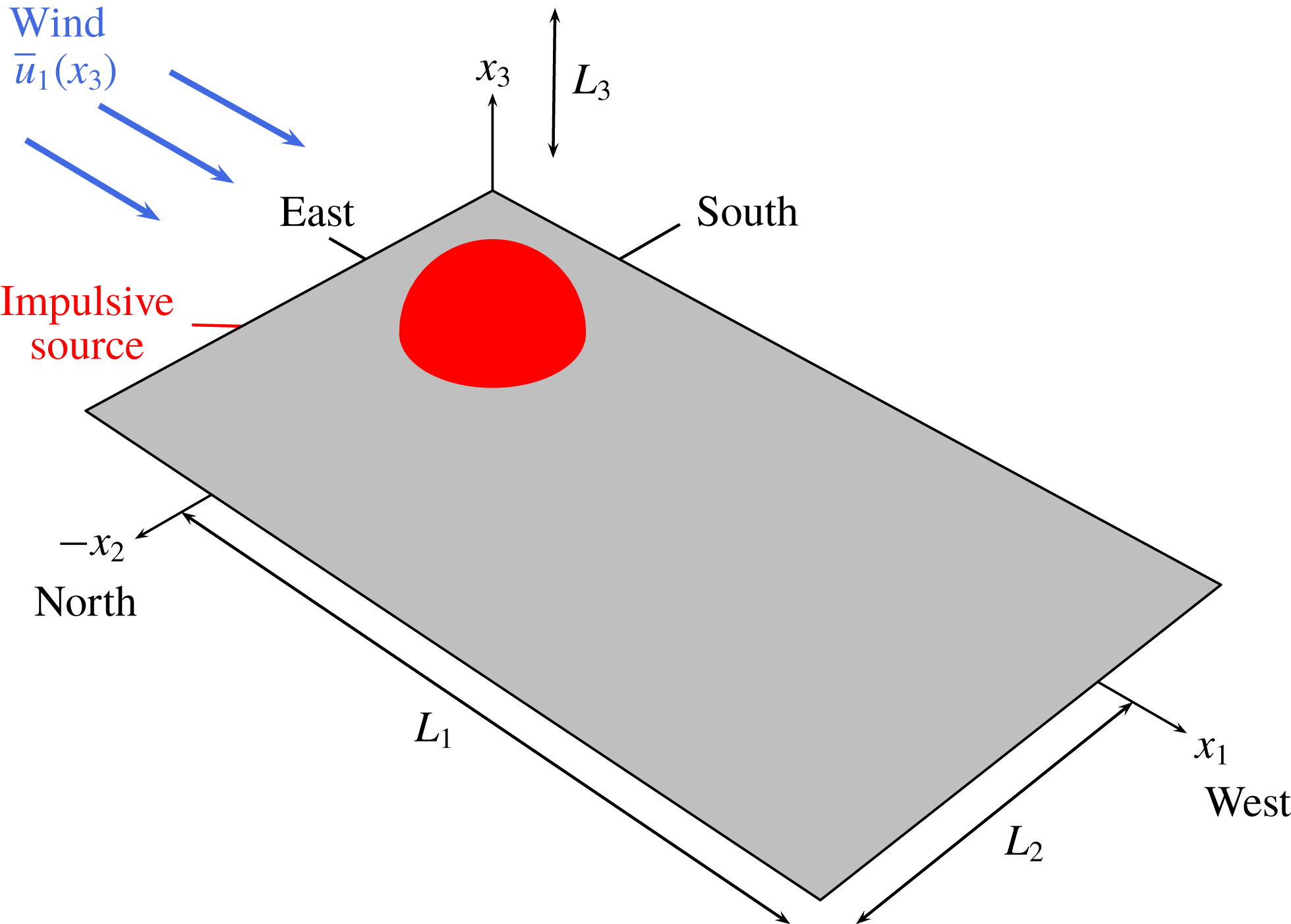
A Cartesian coordinate system
 $Ox_{1}x_{2}x_{3}$
with its origin at ground level and vertical axis
 $x_{3}$
is employed. The Earth’s surface is modelled as a perfectly reflecting flat wall, which is represented by the
 $x_{1}{-}x_{2}$
plane. An infrasonic source is placed at the point
 $O$
. A sketch of the problem is illustrated in figure 1.
Sketch of the physical domain.

2.1 Fluid model
For the purpose of the present investigation, the air in the atmosphere is assumed to behave as a single ideal gas satisfying the equation of state
 $p=\unicode[STIX]{x1D70C}rT$
, where
 $p$
is the pressure,
 $\unicode[STIX]{x1D70C}$
is the fluid density,
 $T$
is the temperature and
 $r=287.06~\text{J}~\text{kg}^{-1}~\text{K}^{-1}$
is the specific gas constant. The speed of sound
 $c$
is given by the relation
 $c=\sqrt{\unicode[STIX]{x1D6FE}rT}$
, where
 $\unicode[STIX]{x1D6FE}=c_{p}/c_{v}=1.4$
represents the ratio of the specific heat capacity at constant pressure
 $c_{p}$
to the specific heat capacity at constant volume
 $c_{v}=c_{p}-r$
. The molar mass and the specific heats are considered constant. As a result, the internal energy
 $e$
and the enthalpy
 $h$
are simply computed as
 $e=c_{v}T$
and
 $h=c_{p}T$
, respectively. The fluid flow is described by the conservative variables
 $[\unicode[STIX]{x1D70C},\unicode[STIX]{x1D70C}u_{1},\unicode[STIX]{x1D70C}u_{2},\unicode[STIX]{x1D70C}u_{3},\unicode[STIX]{x1D70C}e_{t}]$
, where
 $u_{i}$
is the component of the velocity vector in the direction
 $x_{i}$
, for
 $i=1,2,3$
, and
 $e_{t}=e+u_{k}u_{k}/2$
indicates the total specific energy, which is related to the pressure
 $p$
by the relationship
 $p=(\unicode[STIX]{x1D6FE}-1)(\unicode[STIX]{x1D70C}e_{t}-\unicode[STIX]{x1D70C}u_{k}u_{k}/2)$
.
2.2 Initial undisturbed atmosphere
At the instant
 $t=0$
, the initial undisturbed atmosphere is defined as a stationary and stratified medium, with a wind in the
 $x_{1}$
direction
 $$\begin{eqnarray}\bar{\unicode[STIX]{x1D70C}}=\bar{\unicode[STIX]{x1D70C}}(x_{3}),\quad \bar{\unicode[STIX]{x1D70C}}\bar{u}_{i}=\bar{\unicode[STIX]{x1D70C}}(x_{3})\bar{u}_{i}(x_{3}),\quad i=1,2,3,\quad \bar{\unicode[STIX]{x1D70C}}\bar{e}_{t}=\bar{\unicode[STIX]{x1D70C}}(x_{3})\bar{e}_{t}(x_{3}).\end{eqnarray}$$
In the present study, the vertical profiles of the temperature
 $\bar{T}(x_{3})$
and the horizontal wind
 $\bar{u}_{1}(x_{3})$
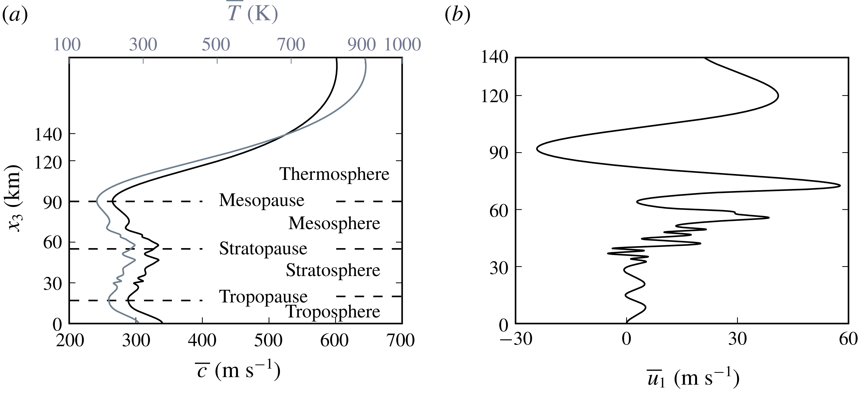
are defined by combining the data measured during the Misty-Picture experiment with empirical models (see Gainville et al. (Reference Gainville, Blanc-Benon, Blanc, Roche, Millet, Le Piver, Despres, Piserchia, Le Pichon, Blanc and Hauchecorne2010) for further details). They are displayed in figures 2(a) and 2(b), respectively. A synthetic nomenclature of the different atmospheric layers is also reported in figure 2(a). The length scale for variations of the initial undisturbed atmosphere is globally higher than around 10 km. Nonetheless, small-scale inhomogeneities are clearly visible in the stratosphere, between 25 and 55 km altitude. Their characteristic length is equal to about 4 km and is close to the acoustic wavelengths
 $\unicode[STIX]{x1D706}$
considered in this study.
(a) Vertical profiles of the speed of sound
 $\bar{c}(x_{3})$
(black line) and of the temperature
 $\bar{T}(x_{3})$
(grey line); (b) mean horizontal wind
 $\bar{u}_{1}(x_{3})$
in the east–west direction versus altitude.

The mean speed of sound
 $\bar{c}(x_{3})$
is computed from the temperature according to the relation
 $\bar{c}(x_{3})=\sqrt{\unicode[STIX]{x1D6FE}r\bar{T}(x_{3})}$
. The pressure profile
 $\bar{p}(x_{3})$
is then obtained by integrating the hydrostatic equilibrium equation
 $$\begin{eqnarray}\frac{\text{d}\bar{p}}{\text{d}x_{3}}=-\bar{\unicode[STIX]{x1D70C}}g=-\frac{g}{r\bar{T}}\bar{p},\end{eqnarray}$$
where
 $g=9.81~\text{m}~\text{s}^{-2}$
is the gravitational acceleration, here assumed to be constant, with the ground-level pressure fixed to
 $\bar{p}_{0}\equiv \bar{p}(0)=101\,325$
Pa. Finally, the density and the specific energy are determined from the expressions
 $\bar{\unicode[STIX]{x1D70C}}=\bar{p}/(r\bar{T})$
and
 $\bar{\unicode[STIX]{x1D70C}}\bar{e}_{t}=\bar{p}/(\unicode[STIX]{x1D6FE}-1)+\bar{\unicode[STIX]{x1D70C}}\bar{u}_{1}^{2}/2$
.
2.3 Governing equations
Sound propagation is governed by the three-dimensional unsteady compressible Navier–Stokes equations, which can be recast as
 $$\begin{eqnarray}\left.\begin{array}{@{}c@{}}\displaystyle \frac{\unicode[STIX]{x2202}\unicode[STIX]{x1D70C}}{\unicode[STIX]{x2202}t}+\frac{\unicode[STIX]{x2202}(\unicode[STIX]{x1D70C}u_{j})}{\unicode[STIX]{x2202}x_{j}}=\unicode[STIX]{x1D6EC}_{\unicode[STIX]{x1D70C}},\\ \displaystyle \frac{\unicode[STIX]{x2202}(\unicode[STIX]{x1D70C}u_{i})}{\unicode[STIX]{x2202}t}+\frac{\unicode[STIX]{x2202}(\unicode[STIX]{x1D70C}u_{i}u_{j})}{\unicode[STIX]{x2202}x_{j}}=-\frac{\unicode[STIX]{x2202}p^{\prime }}{\unicode[STIX]{x2202}x_{i}}+\frac{\unicode[STIX]{x2202}\unicode[STIX]{x1D70F}_{ij}^{\star }}{\unicode[STIX]{x2202}x_{j}}-\unicode[STIX]{x1D70C}^{\prime }g\unicode[STIX]{x1D6FF}_{i3},\\ \displaystyle \frac{\unicode[STIX]{x2202}(\unicode[STIX]{x1D70C}e_{t})}{\unicode[STIX]{x2202}t}+\frac{\unicode[STIX]{x2202}(\unicode[STIX]{x1D70C}e_{t}u_{j})}{\unicode[STIX]{x2202}x_{j}}=-\frac{\unicode[STIX]{x2202}\left(p^{\prime }u_{j}\right)}{\unicode[STIX]{x2202}x_{j}}-\bar{p}\frac{\unicode[STIX]{x2202}u_{j}}{\unicode[STIX]{x2202}x_{j}}-\frac{\unicode[STIX]{x2202}q_{j}^{\star }}{\unicode[STIX]{x2202}x_{j}}+\frac{\unicode[STIX]{x2202}(u_{i}\unicode[STIX]{x1D70F}_{ij}^{\star })}{\unicode[STIX]{x2202}x_{j}}-\unicode[STIX]{x1D70C}^{\prime }gu_{3}+\unicode[STIX]{x1D6EC}_{\unicode[STIX]{x1D70C}e_{t}},\end{array}\right\}\end{eqnarray}$$
where
 $p^{\prime }=p-\bar{p}$
is the pressure perturbation,
 $\unicode[STIX]{x1D70C}^{\prime }=\unicode[STIX]{x1D70C}-\bar{\unicode[STIX]{x1D70C}}$
is the density perturbation,
 $\unicode[STIX]{x1D70F}_{ij}^{\star }$
is the viscous stress tensor,
 $q_{i}^{\prime }$
is the heat flux,
 $\unicode[STIX]{x1D6EC}_{\unicode[STIX]{x1D70C}}$
and
 $\unicode[STIX]{x1D6EC}_{\unicode[STIX]{x1D70C}e_{t}}$
are two source-forcing terms and
 $\unicode[STIX]{x1D6FF}_{ij}$
is the Kronecker symbol. Note that, in keeping with Marsden et al. (Reference Marsden, Bailly and Bogey2014), the hydrostatic equilibrium condition
 $\text{d}\bar{p}/\text{d}x_{3}=-\bar{\unicode[STIX]{x1D70C}}g$
is here subtracted from the Navier–Stokes equations in order to bypass its high-precision computation at each time step. Moreover, because of the non-vanishing terms
 $\unicode[STIX]{x2202}\bar{\unicode[STIX]{x1D70F}}_{12}/\unicode[STIX]{x2202}x_{1}$
and
 $\unicode[STIX]{x2202}\bar{q}_{2}/\unicode[STIX]{x2202}x_{2}$
, the initial undisturbed atmosphere, determined from experimental data, is not fully consistent with the Navier–Stokes equations and thus would tend to evolve in time. To avoid the diffusion of the mean flow during the acoustic propagation, the viscous and the thermal conduction terms are calculated using the perturbed variables
 $u_{i}^{\prime }=u_{i}-\bar{u}_{i}$
and
 $T^{\prime }=T-\bar{T}$
. More specifically, the viscous stress tensor and the heat flux are computed respectively as
 $$\begin{eqnarray}\unicode[STIX]{x1D70F}_{ij}^{\star }=\unicode[STIX]{x1D707}\left(\frac{\unicode[STIX]{x2202}u_{i}^{\prime }}{\unicode[STIX]{x2202}x_{j}}+\frac{\unicode[STIX]{x2202}u_{j}^{\prime }}{\unicode[STIX]{x2202}x_{i}}-\frac{2}{3}\frac{\unicode[STIX]{x2202}u_{k}^{\prime }}{\unicode[STIX]{x2202}x_{k}}\unicode[STIX]{x1D6FF}_{ij}\right)\end{eqnarray}$$
and
 $$\begin{eqnarray}q_{i}^{\star }=-\frac{\unicode[STIX]{x1D707}c_{p}}{Pr}\frac{\unicode[STIX]{x2202}T^{\prime }}{\unicode[STIX]{x2202}x_{i}},\end{eqnarray}$$
where
 $\unicode[STIX]{x1D707}$
is the dynamic viscosity and
 $Pr=0.72$
is the fluid’s Prandtl number. Finally, the dynamic viscosity is given by the expression
 $$\begin{eqnarray}\unicode[STIX]{x1D707}(T)=\unicode[STIX]{x1D707}_{ref}\left(\frac{T}{T_{ref}}\right)^{3/2}\frac{T_{ref}+T_{S}}{T+T_{S}},\end{eqnarray}$$
where
 $\unicode[STIX]{x1D707}_{ref}=1.8192\times 10^{-5}$
Pa s,
 $T_{ref}=293.15$
K and
 $T_{S}=117$
K (Sutherland & Bass Reference Sutherland and Bass2004, Reference Sutherland and Bass2006).
2.4 Infrasonic source
The infrasonic source is implemented through the following forcing terms of the continuity and energy conservation equations:
 $$\begin{eqnarray}\displaystyle \left.\begin{array}{@{}c@{}}\unicode[STIX]{x1D6EC}_{\unicode[STIX]{x1D70C}e_{t}}(\boldsymbol{x},t)={\mathcal{A}}_{s}\sin (\unicode[STIX]{x1D714}_{s}t)[1-\cos (2\unicode[STIX]{x1D714}_{s}t)]\unicode[STIX]{x1D6F1}_{[0,\unicode[STIX]{x03C0}/\unicode[STIX]{x1D714}_{s}]}(t)\text{e}^{-\text{log}(2)\Vert \boldsymbol{x}\Vert ^{2}/b_{s}^{2}}\\ \unicode[STIX]{x1D6EC}_{\unicode[STIX]{x1D70C}}(\boldsymbol{x},t)={\displaystyle \frac{\unicode[STIX]{x1D6FE}-1}{\bar{c}^{2}(x_{3})}}\unicode[STIX]{x1D6EC}_{\unicode[STIX]{x1D70C}e_{t}}(\boldsymbol{x},t),\end{array}\right\} & & \displaystyle\end{eqnarray}$$
where
 ${\mathcal{A}}_{s}=3\times 10^{5}~\text{J}~\text{m}^{-3}~\text{s}^{-1}$
is the source strength,
 $f_{s}=\unicode[STIX]{x1D714}_{s}/(2\unicode[STIX]{x03C0})=0.2$
Hz the source frequency,
 $b_{s}=360$
m the half-width and
 $\unicode[STIX]{x1D6F1}_{[0,\unicode[STIX]{x03C0}/\unicode[STIX]{x1D714}_{s}]}(t)$
the rectangle function, equal to
 $1$
in the interval
 $[0,\unicode[STIX]{x03C0}/\unicode[STIX]{x1D714}_{s}]$
and
 $0$
otherwise. As explained in appendix A, the functions
 $\unicode[STIX]{x1D6EC}_{\unicode[STIX]{x1D70C}e_{t}}$
and
 $\unicode[STIX]{x1D6EC}_{\unicode[STIX]{x1D70C}}$
are designed in order to obtain a blast wave, typical of explosions (Whitham Reference Whitham1974), close to the origin of the domain.
2.5 About the main hypotheses of the present propagation model
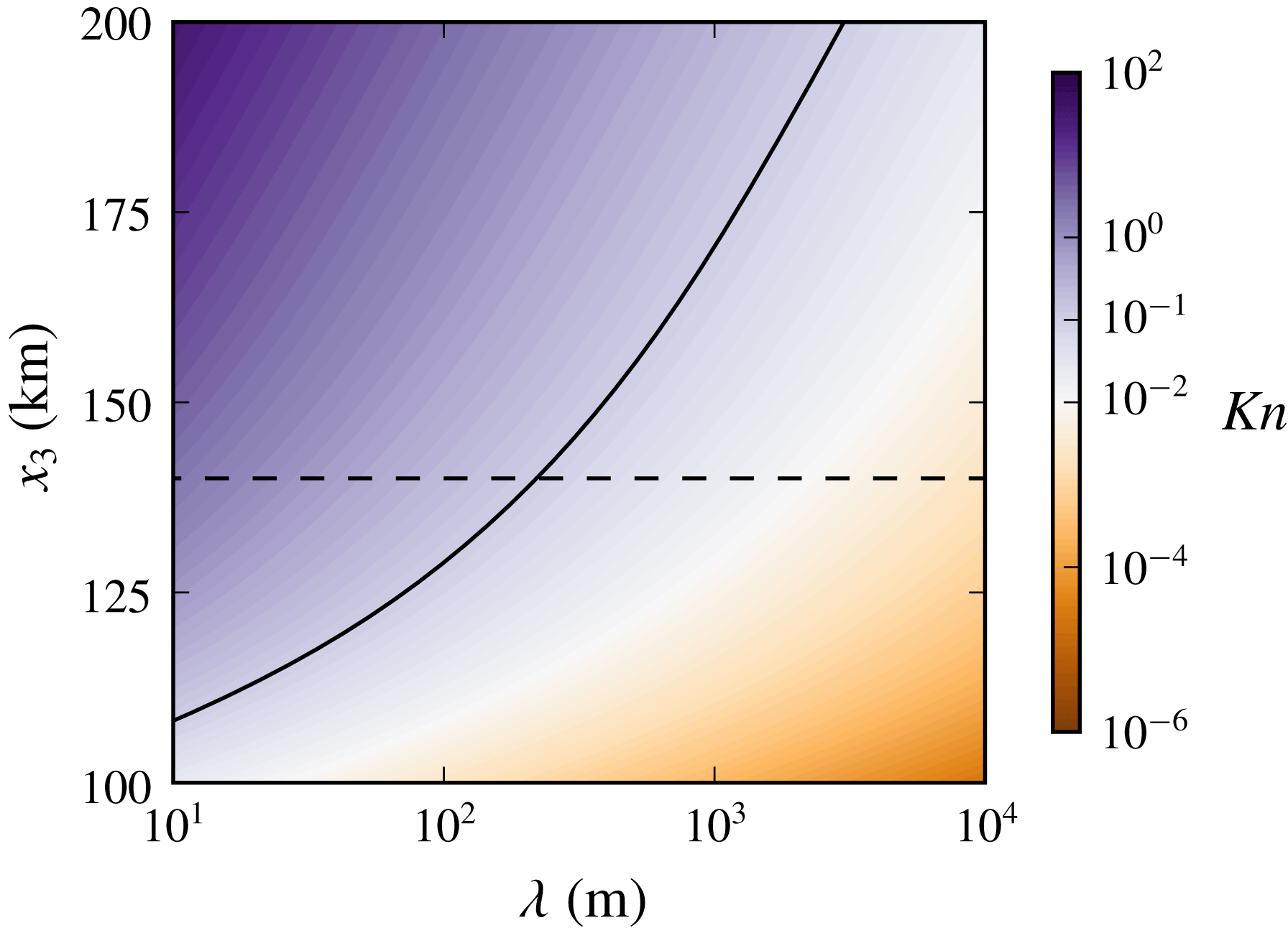
The present propagation model, based on the three-dimensional compressible unsteady Navier–Stokes equations, rests upon the continuum hypothesis (Batchelor Reference Batchelor2012), which is valid when the characteristic wavelength
 $\unicode[STIX]{x1D706}$
is large enough compared to the free mean path
 $\ell$
. This latter is equal to about
 $10^{-7}$
m at ground level, but can reach significant values in the thermosphere. The typical behaviour of the Knudsen number
 $Kn=\ell /\unicode[STIX]{x1D706}$
in the atmosphere is shown in figure 3 as a function of the wavelength
 $\unicode[STIX]{x1D706}$
and of the altitude
 $x_{3}$
. The conventional limit of validity,
 $Kn=0.1$
, is also reported. Clearly, becoming irrelevant at altitudes higher than 140 km for values of
 $\unicode[STIX]{x1D706}$
lower than about 200 m, the continuum hypothesis is verified for the range of wavelengths of interest in this study.
Knudsen number
 $Kn$
as a function of the wavelength
 $\unicode[STIX]{x1D706}$
and of the altitude
 $x_{3}$
. The solid and dashed lines represent the level set
 $Kn=0.1$
and the limit of the physical domain of interest, respectively.

Another underlying assumption of the present model is the negligibility of relaxation effects, but, as shown by Sabatini et al. (Reference Sabatini, Marsden, Bailly and Gainville2016b ), non-equilibrium phenomena mainly affect tropospheric and stratospheric waves of frequency greater than 1 Hz.
3 Numerical algorithm
System (2.3) is solved on a Cartesian grid using a high-order finite-difference time-domain method.
3.1 Computational domain
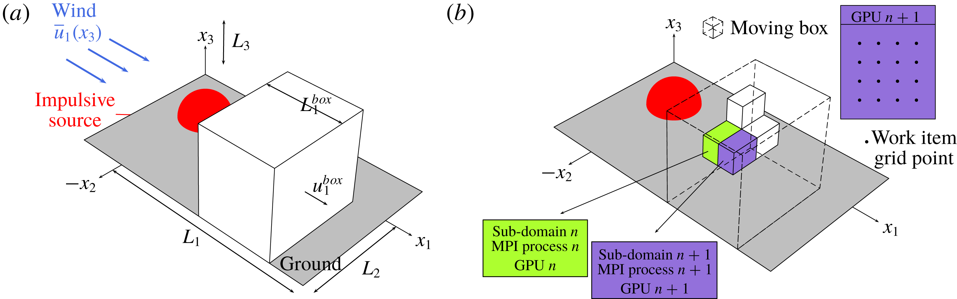
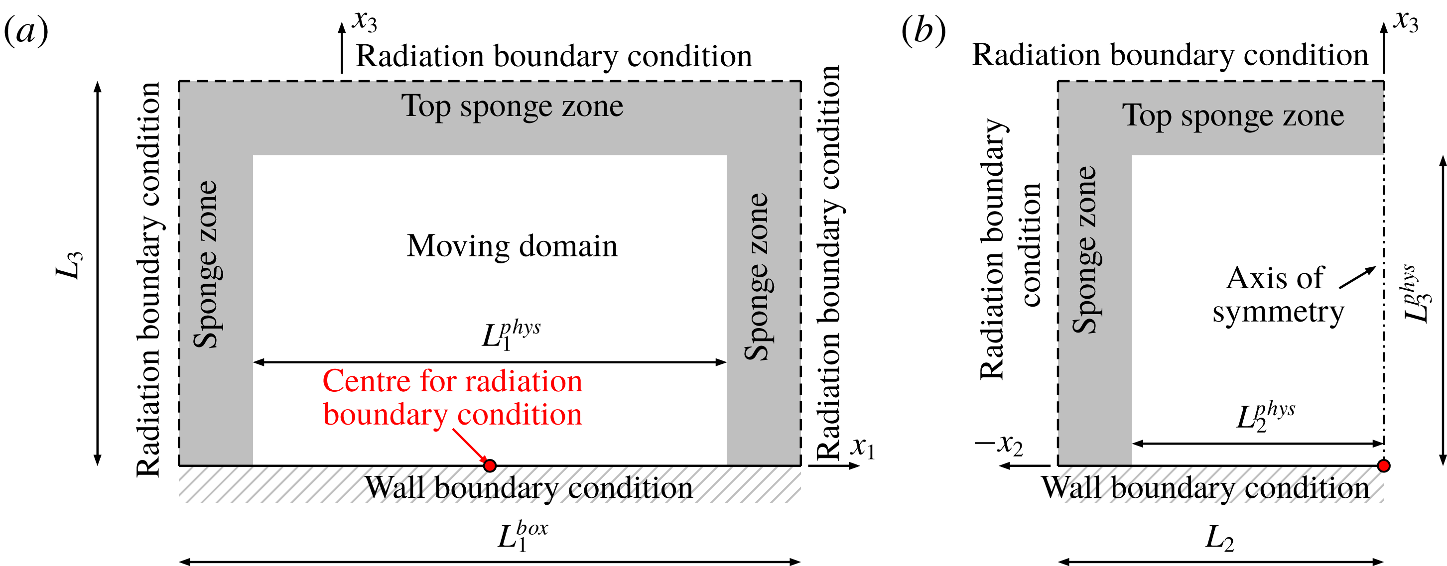
The maximum number of mesh points being constrained by the computer memory, a moving frame is employed (Salomons, Blumrich & Heimann Reference Salomons, Blumrich and Heimann2002; Sabatini et al.
Reference Sabatini, Marsden, Bailly and Gainville2015; de Groot-Hedlin Reference de Groot-Hedlin2016). System (2.3) is solved only in a narrow region which moves along the
 $x_{1}$
axis and follows the acoustic wavefront. A schematic illustration of the technique is provided in figure 4(a). The physical domain of interest is a parallelepiped of sizes
 $450$
km,
 $L_{2}^{phys}=90$
km,
 $L_{3}^{phys}=140$
km along the
 $x_{1}$
,
 $x_{2}$
,
 $x_{3}$
axes, respectively, while the moving window covers a distance of
 $L_{1}^{phys}=220$
km in the
 $x_{1}$
direction. As displayed in figures 5(a) and 5(b), the physical domain
 $L_{1}^{phys}\times L_{2}^{phys}\times L_{3}^{phys}$
is surrounded by sponge zones where particular numerical techniques are used in order for outgoing waves to leave the computational frame without significant reflections. Moreover, since no wind is considered in the
 $x_{2}$
direction and the source forcing terms (2.7) depends only on the radial distance
 $\Vert \boldsymbol{x}\Vert$
, the acoustic field is symmetric across the
 $x_{1}{-}x_{3}$
plane. Accordingly, with reference to figure 4(a), System (2.3) is solved only for negative values of the coordinate
 $x_{2}$
.
3.2 Numerical schemes
At inner points, the spatial derivatives are computed using an explicit fourth-order 11-point stencil finite-difference scheme optimized to reduce dispersion for wavelengths shorter than about five grid spacings (Bogey & Bailly Reference Bogey and Bailly2004). Close to the boundaries of the computational domain, optimized 11-point stencil non-centred finite-difference schemes are employed (Berland et al. Reference Berland, Bogey and Bailly2007). The time integration is carried out by a six-step second-order low-storage Runge–Kutta algorithm (Bogey & Bailly Reference Bogey and Bailly2004).
At the end of each time step, spatial low pass filtering is performed on the perturbations of conservative variables
 $U^{\prime }=[\unicode[STIX]{x1D70C}-\bar{\unicode[STIX]{x1D70C}},\unicode[STIX]{x1D70C}u_{1}-\bar{\unicode[STIX]{x1D70C}}\bar{u}_{1},\unicode[STIX]{x1D70C}u_{2}-\bar{\unicode[STIX]{x1D70C}}\bar{u}_{2},\unicode[STIX]{x1D70C}u_{3}-\bar{\unicode[STIX]{x1D70C}}\bar{u}_{3},\unicode[STIX]{x1D70C}e_{t}-\bar{\unicode[STIX]{x1D70C}}\bar{e}_{t}]$
, in order to damp out grid-to-grid oscillations and ensure numerical stability. For this purpose, an explicit sixth-order 11-point stencil filter, designed to remove fluctuations discretized by less than four grid points per wavelength, while leaving larger wavelengths unaffected, is employed at inner nodes (Bogey et al.
Reference Bogey, Cacqueray and Bailly2009). Close to the boundaries of the computational frame, optimized 11-point stencil non-centred filters are applied instead (Berland et al.
Reference Berland, Bogey and Bailly2007). Additionally, in order to handle the acoustic shocks generated during the propagation, the shock-capturing procedure developed by Bogey et al. (Reference Bogey, Cacqueray and Bailly2009) is used in conjunction with the new shock detector proposed by Sabatini et al. (Reference Sabatini, Marsden, Bailly and Bogey2016a
).
(a) Sketch of the computational domain. (b) Schematic illustration of the two-level parallelism of the present solver for the Navier–Stokes equations.

3.3 Boundary conditions and sponge zones
The flow field near a wall can be decomposed, in the linear regime, into the sum of three different waves, namely the vorticity, the entropy and the acoustic modes. The first two waves have appreciable amplitudes only in the vicinity of the wall, up to distances of the order of the acoustic boundary layer thickness
 $\unicode[STIX]{x1D6FF}_{\unicode[STIX]{x1D707}}=\sqrt{2\bar{\unicode[STIX]{x1D707}}/(2\unicode[STIX]{x03C0}f\bar{\unicode[STIX]{x1D70C}})}$
. Close to the Earth’s surface,
 $\unicode[STIX]{x1D6FF}_{\unicode[STIX]{x1D707}}$
is equal to about
 $1$
cm for a frequency
 $f$
of
 $0.2$
Hz and a wavelength
 $\unicode[STIX]{x1D706}$
of
 $1.7$
km, i.e.
 $\unicode[STIX]{x1D6FF}_{\unicode[STIX]{x1D707}}=1.7\times 10^{-6}\,\unicode[STIX]{x1D706}$
. Understandably, in the present simulation, the flow field at ground level is dominated by the acoustic mode, which alone satisfies a no-slip boundary condition. Accordingly, at nodes on the Earth’s surface, only the vertical velocity
 $u_{3}$
is set to zero, whereas no condition is imposed on the other conservative variables, which are advanced in time by solving the Navier–Stokes equations.
At grid points on the other boundaries, radiation conditions, as formulated by Bogey & Bailly (Reference Bogey and Bailly2002), are implemented. In order to diminish the amplitude of the outgoing waves reaching the boundaries of the computational domain, in the sponge zones, a Laplacian filter is employed. Its strength gradually augments from zero, at the beginning of the sponge layer, to a maximum value at the extremity of the frame. Along the
 $x_{2}$
and
 $x_{3}$
axes, the reduction of the wave amplitude is further enhanced by the increase of the grid spacing. A supplementary technique is finally required in the top numerical sponge zone. Due to gravity stratification, the ratio of pressure fluctuations to ambient pressure would tend to amplify with altitude. Therefore, as proposed by Marsden et al. (Reference Marsden, Bailly and Bogey2014), the gravity profile in the top sponge layer is progressively reduced from
 $g$
to
 $-g$
.
Projections of the moving domain on the (a)
 $x_{1}{-}x_{3}$
and (b)
 $x_{2}{-}x_{3}$
planes.

3.4 Informatic implementation and numerical parameters
The numerical algorithm has been written in C/C
 $++$
with a two-level parallelism, allowing one to exploit the excellent performance of GPU clusters (Jacobsen & Senocak Reference Jacobsen and Senocak2013). The moving box is split into several sub-domains, each of which is handled by an MPI process. In its turn, each MPI node drives, thanks to OpenCL kernels, a GPU. A GPU can be seen as an ensemble of work-groups, each of which is made of processing elements or work-items. The same program or kernel (such as the kernel computing the partial derivative along an axis) can be executed on all the processing elements at the same time. Hence, each work-item can handle all the operations for a single grid node (cf. figure 4
b).
The moving box is divided into
 $6\times 8\times 3=144$
sub-domains, each of which contains
 $448\times 64\times 512$
grid points. The total number of mesh nodes is about
 $2.11$
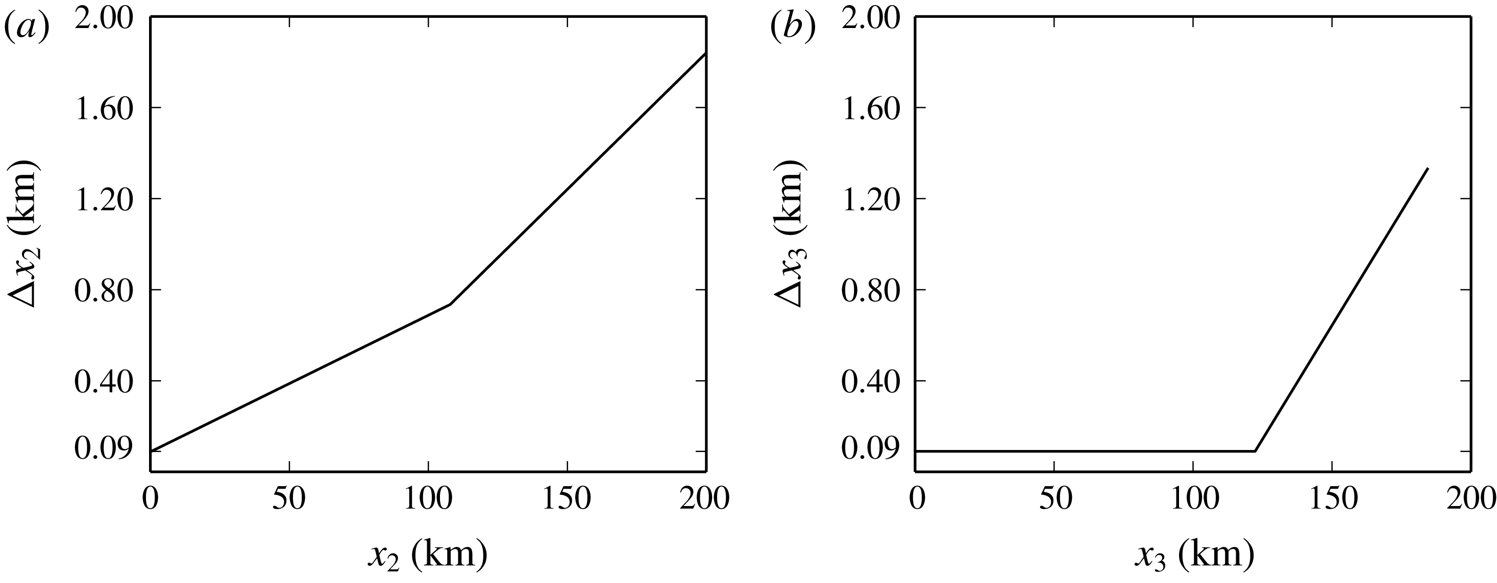
billion. The step size is constant and equal to
 $\unicode[STIX]{x0394}x_{1}=90$
m on the
 $x_{1}$
axis. On the
 $x_{2}$
axis, the grid is stretched with a rate of
 $0.6\,\%$
from
 $x_{2}=1$
km to
 $x_{2}=105$
km and with a rate equal to
 $1.2\,\%$
beyond. On the
 $x_{3}$
axis, the spatial step is of
 $90$
up to
 $125$
km, and then increases at a rate of
 $2\,\%$
. The variations of the mesh spacings
 $\unicode[STIX]{x0394}x_{2}$
and
 $\unicode[STIX]{x0394}x_{3}$
are represented in figures 6(a) and 6(b).
The time step is set equal to
 $0.0699$
s and the computation is carried out up to
 $1600$
s, corresponding to 23 000 iterations. The Courant–Friedrichs–Lewy and Fourier numbers computed using the speed of sound and the kinematic viscosity at the top of the physical domain along the vertical axis are
 $0.4$
and
 $0.07$
, respectively.
The present numerical simulation was run on the hybrid nodes of the Curie supercomputer, located in the Commissariat à l’énergie atomique et aux énergies alternatives (CEA, France), and
 $144$
Nvidia M2090 T20A GPUs were used.
Variations of the grid spacing along (a) the
 $x_{2}$
axis and (b) the
 $x_{3}$
axis.

4 Results
As demonstrated by Bergmann (Reference Bergmann1946), the amplitude of the pressure perturbation
 $p^{\prime }$
evolves proportionally to the square root of the ambient density
 $\bar{\unicode[STIX]{x1D70C}}$
. Therefore, the normalized pressure fluctuation
 $\unicode[STIX]{x1D6F7}(\boldsymbol{x},t)=p^{\prime }(\boldsymbol{x},t)/\sqrt{\bar{\unicode[STIX]{x1D70C}}(x_{3})}$
is analysed along with the overpressure
 $p^{\prime }$
. In addition, the signature of
 $p^{\prime }$
and
 $\unicode[STIX]{x1D6F7}$
are studied in the frequency domain, by considering the one-sided energy spectral density
 $$\begin{eqnarray}{\mathcal{E}}_{\unicode[STIX]{x1D712}}(\boldsymbol{x},f)=2\left|\int _{-\infty }^{+\infty }\unicode[STIX]{x1D712}(\boldsymbol{x},t)\text{e}^{\text{i}2\unicode[STIX]{x03C0}ft}\,\text{d}t\right|^{2},\quad f\in \mathbb{R}^{+},\unicode[STIX]{x1D712}=p^{\prime },\unicode[STIX]{x1D6F7}.\end{eqnarray}$$
4.1 General description of the acoustic field
The three-dimensional normalized pressure fields
 $\unicode[STIX]{x1D6F7}$
obtained at different instants of time are displayed in figure 7(a–i). The black box represents the computational moving frame, whereas the red box indicates the physical domain of interest. The colour level ranges from
 $-10~\text{Pa}~\text{kg}^{-1/2}~\text{m}^{3/2}$
(blue) to
 $+10~\text{Pa}~\text{kg}^{-1/2}~\text{m}^{3/2}$
(red). This interval is chosen in order to visualize the various infrasonic phases, which may have very different amplitudes. Successive points on the axes
 $x_{1}$
,
 $x_{2}$
and
 $x_{3}$
are
 $100$
km distant.
Three-dimensional normalized pressure field
 $\unicode[STIX]{x1D6F7}$
obtained for different instants of time. The black box represents the computational moving frame, whereas the red box is the physical domain of interest. The times are (a)
 $t_{1}=146.79$
s, (b)
 $t_{2}=216.69$
s, (c)
 $t_{3}=356.49$
s, (d)
 $t_{4}=566.19$
s, (e)
 $t_{5}=775.89$
s, (f)
 $t_{6}=1055.49$
s, (g)
 $t_{7}=1265.19$
s, (h)
 $t_{8}=1404.99$
s, (i)
 $t_{9}=1544.79$
s.

Near the source location, a spherical wavefront is observed. However, as a result of the vertical gradients of the speed of sound and of the horizontal wind, the infrasonic wave is continuously deformed during the propagation. At the instant
 $t_{2}$
, partial reflections start being observed between
 $25$
and
 $55$
km altitude. They are induced by variations of the speed of sound and of the wind of length scale comparable to the acoustic wavelength. The amplitude of these reflections appears strengthened at the instant
 $t_{3}$
. Moreover, because of nonlinear effects, the acoustic wavefront lengthens while propagating towards the thermosphere. At the instant
 $t_{4}$
, the infrasonic wave is refracted back towards the Earth’s surface. In addition, part of the wavefront leaves the domain through the top boundary. The computational frame starts moving between times
 $t_{4}$
and
 $t_{5}$
. At the instant
 $t_{5}$
, the signal at ground level, between
 $x_{1}=200$
km and
 $x_{1}=250$
km on the
 $x_{1}$
axis, is a superposition of partial reflections and stratospheric returns, while a thermospheric phase is reaching the Earth’s surface at about
 $x_{1}=180$
km distance from the source location. Furthermore, part of the wavefront leaves the moving window through the plane
 $x_{2}=-L_{2}$
with a negligible level of spurious reflection. At the instant
 $t_{6}$
, the thermospheric phase is clearly visible on the ground at around
 $x_{1}=250$
km. At successive instants, the pressure field becomes more and more complex and a multitude of arrivals are recorded at the Earth’s surface. The computational box stops moving just after reaching the boundary of the physical domain, between times
 $t_{6}$
and
 $t_{7}$
. The simulation ends up once the wavefront exits the frame.
4.2 The signal in the near field
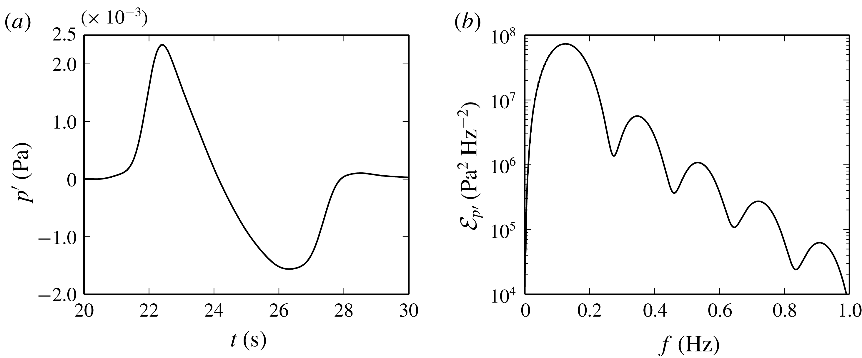
The pressure perturbation
 $p^{\prime }$
recorded on the
 $x_{1}$
axis at
 $x_{1}=7.92$
km and the corresponding energy spectral density
 ${\mathcal{E}}_{p^{\prime }}$
are plotted in figure 8(a,b). The pressure signal in the near field exhibits an N-waveform, has a maximum amplitude of
 $2330$
Pa and a total duration of
 $6$
s. The central frequency is equal to about
 $0.13$
Hz and corresponds to a wavelength of
 $2.6$
km.
(a) Pressure perturbation
 $p^{\prime }$
recorded on the
 $x_{1}$
axis at
 $x_{1}=7.92$
km and (b) corresponding energy spectral density
 ${\mathcal{E}}_{p^{\prime }}$
.

4.3 Nonlinear effects in the upper atmosphere
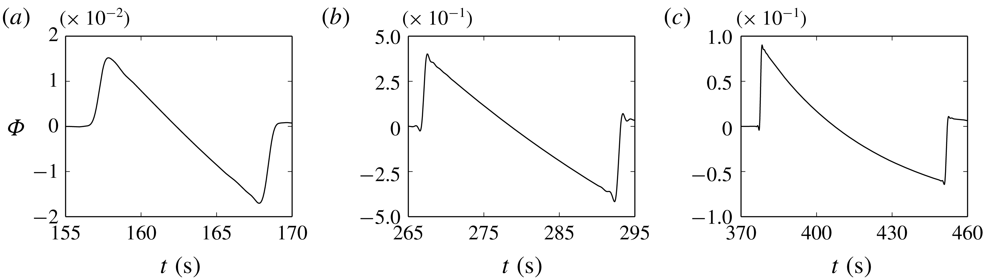
The normalized pressure perturbations
 $\unicode[STIX]{x1D6F7}$
recorded along the vertical axis
 $x_{3}$
at three different altitudes are plotted in figure 9(a–c). At
 $x_{3}=50$
km, an N-shaped signal with a period of
 $12$
s is observed. As a result of nonlinearities, the N-wave lengthens while propagating towards the upper atmosphere, its duration being equal to about
 $26$
and
 $75$
s at
 $x_{3}=90$
and
 $130$
km altitude, respectively. A diminution of the amplitude associated with the increase of the wave period is observed as well. Moreover, at
 $x_{3}=130$
km, the central part of the N-wave is found to be curved. This result is in disagreement with the weakly nonlinear ray theory, according to which an N-wave should conserve its shape during the propagation. The weakly nonlinear ray theory rests upon the assumption that the amplitude of the signal
 $p^{\prime }$
remains at least one order of magnitude smaller than the atmospheric pressure
 $\bar{p}$
, that is,
 $p^{\prime }<0.1\,\bar{p}$
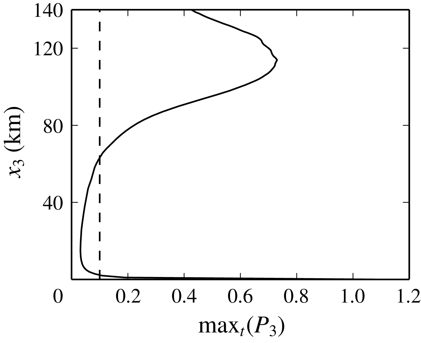
(for instance, see Whitham (Reference Whitham1974)). As illustrated in figure 10, where the maximum in time of the ratio
 $P_{3}(x_{3},t)=p^{\prime }(x_{1}=0,x_{2}=0,x_{3},t)/\bar{p}(x_{3})$
is plotted as a function of the altitude
 $x_{3}$
, the hypothesis
 $\max _{t}(P_{3})<0.1$
is however not verified near the source as well as in the thermosphere. As an example,
 $\max _{t}(P_{3})$
is equal to about
 $0.7$
at
 $x_{3}=114$
km altitude. Therefore, the nonlinear effects cannot be considered weak in the present simulation. To the best of the authors’ knowledge, a model for moderate amplitude waves in a variable atmosphere is currently not available. Qualitative insights into the understanding of the aforesaid signal distortion can nevertheless be gained through a closer analysis of the propagation of one-dimensional plane waves in a homogeneous medium at rest. First, let it be assumed that the viscous and the thermal conduction terms are negligibly small. Second, with
 $x_{3}$
the propagation direction, let it be supposed that the specific entropy
 $s$
is constant,
 $s=\bar{s}$
, and that the velocity
 $u_{3}=u_{3}^{\prime }$
is a single-valued function of the pressure
 $p$
. According to Whitham (Reference Whitham1974), the evolution of a right-running signal is then described by the following nonlinear partial differential equation:
 $$\begin{eqnarray}\frac{\unicode[STIX]{x2202}p^{\prime }}{\unicode[STIX]{x2202}t}+(u_{3}+c)\frac{\unicode[STIX]{x2202}p^{\prime }}{\unicode[STIX]{x2202}x_{3}}=0,\end{eqnarray}$$
with
 $p=\bar{p}(\unicode[STIX]{x1D70C}/\bar{\unicode[STIX]{x1D70C}})^{\unicode[STIX]{x1D6FE}}$
,
 $c=\sqrt{\unicode[STIX]{x1D6FE}p/\unicode[STIX]{x1D70C}}$
and
 $u_{3}=2(c-\bar{c})/(\unicode[STIX]{x1D6FE}-1)$
. Writing the sum
 $(u_{3}+c)$
as a function of the pressure
 $p$
and expanding it for
 $p^{\prime }/\bar{p}\rightarrow 0$
yields
 $$\begin{eqnarray}\frac{\unicode[STIX]{x2202}p^{\prime }}{\unicode[STIX]{x2202}t}+\bar{c}\left[1+\frac{\unicode[STIX]{x1D6FD}}{\bar{\unicode[STIX]{x1D70C}}\bar{c}^{2}}\,p^{\prime }-\frac{\unicode[STIX]{x1D6FD}^{2}}{2\bar{\unicode[STIX]{x1D70C}}^{2}\bar{c}^{4}}\,{p^{\prime }}^{2}+\text{h.o.t.}\right]\frac{\unicode[STIX]{x2202}p^{\prime }}{\unicode[STIX]{x2202}x_{3}}=0,\end{eqnarray}$$
where
 $\unicode[STIX]{x1D6FD}=(\unicode[STIX]{x1D6FE}+1)/2$
is the nonlinear parameter. In the presence of shock waves, the previous hypotheses on the specific entropy
 $s$
and on the velocity
 $u_{3}$
are not verified. However, it can be shown that, at a discontinuity, the relations
 $s-\bar{s}=0$
and
 $u_{3}=u_{3}^{\prime }=2(c-\bar{c})/(\unicode[STIX]{x1D6FE}-1)$
are valid up to the third order in
 $p^{\prime }/\bar{p}$
when
 $p^{\prime }/\bar{p}$
tends to
 $0$
(Whitham Reference Whitham1974). Therefore, equation (4.3) can still be employed in the presence of small or moderate amplitude shocks. When only the first two terms of the Taylor series for
 $(u_{3}+c)$
are retained,
 $u_{3}+c=\bar{c}+\unicode[STIX]{x1D6FD}p^{\prime }/(\bar{\unicode[STIX]{x1D70C}}\bar{c})$
, the classical Burgers equation is recovered. Ray theory is entirely based on an extension of this latter equation to inhomogeneous media (for instance, see Sabatini et al. (Reference Sabatini, Marsden, Bailly and Gainville2016b
) and references therein). In the case of the Burgers equation, an N-wave conserves its shape as a consequence of the linearity in
 $p^{\prime }$
of the first-order approximation of
 $(u_{3}+c)$
. The central part of the waveform remains straight and only a variation of slope can be observed during the propagation. The curvature of the signals recorded in the thermosphere might be thus attributed to high-order terms in
 $p^{\prime }$
, which cannot be neglected beyond a certain altitude. A similar discussion of the distortion of high-amplitude N-waves can be found in Inoue & Yano (Reference Inoue and Yano1997).
Normalized pressure signals
 $\unicode[STIX]{x1D6F7}$
recorded on the
 $x_{3}$
axis at (a)
 $x_{3}=50$
km, (b)
 $x_{3}=90$
km and (c)
 $x_{3}=130$
km.

Maximum of the ratio
 $P_{3}$
between the pressure perturbation
 $p^{\prime }$
on the
 $x_{3}$
axis and the atmospheric pressure
 $\bar{p}$
. The dashed line represents the conventional limit of validity of the weakly nonlinear ray theory,
 $\max _{t}(P_{3})=0.1$
.

Spectrum
 ${\mathcal{E}}_{\unicode[STIX]{x1D6F7},3}$
of the signals
 $\unicode[STIX]{x1D6F7}$
recorded along the
 $x_{3}$
axis.

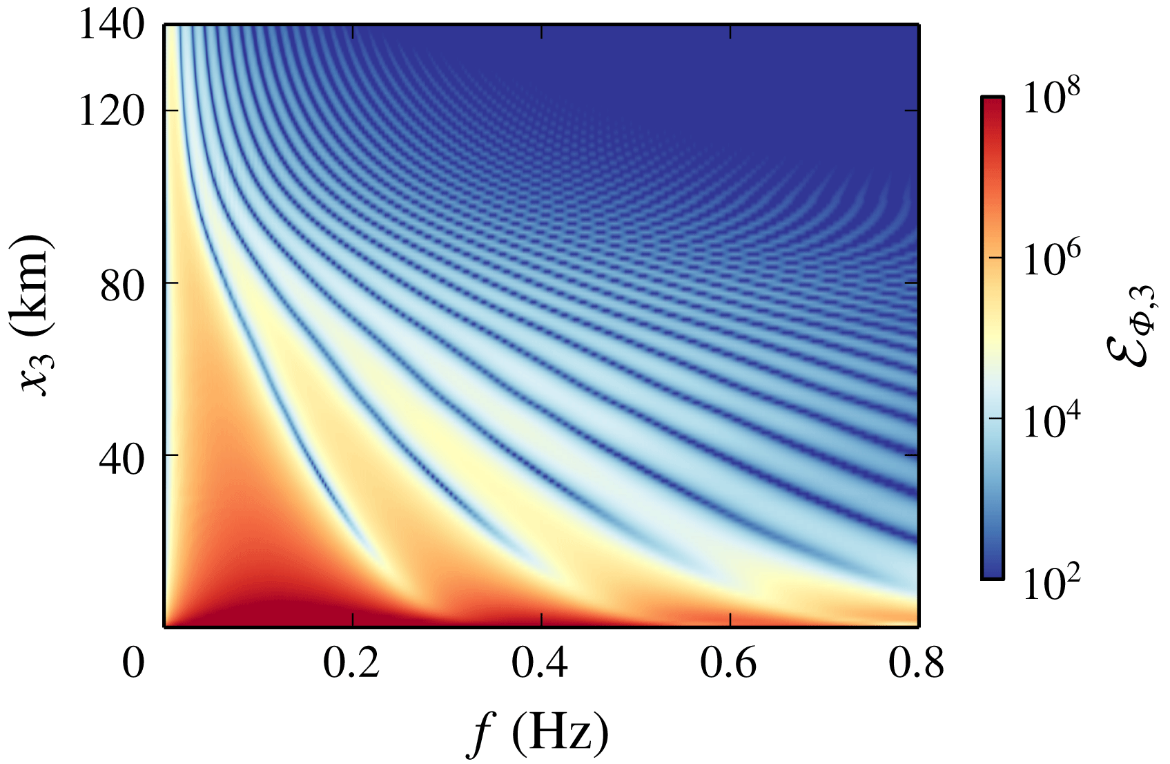
The energy spectral density
 ${\mathcal{E}}_{\unicode[STIX]{x1D6F7},3}(x_{3},f)={\mathcal{E}}_{\unicode[STIX]{x1D6F7}}(0,0,x_{3},f)$
of the signals
 $\unicode[STIX]{x1D6F7}$
recorded along the
 $x_{3}$
axis is finally plotted in figure 11 as a function of the frequency
 $f$
and of the altitude
 $x_{3}$
. The nonlinear lengthening of the N-wave leads to a shift of the spectrum towards very low frequencies. Therefore, throughout the propagation, most of the energy is carried by spectral components which are weakly affected by the viscous and the thermal conduction terms. Dissipative effects only influence the shock region, but play a minor role in the waveform.
Acoustic field
 $\unicode[STIX]{x1D6F7}$
on the
 $x_{1}{-}x_{3}$
plane at (a)
 $t_{3}$
, (c)
 $t_{5}$
and (e)
 $t_{7}$
. Pressure signals
 $p^{\prime }$
recorded on the
 $x_{1}$
axis at (b)
 $x_{1}=100$
km, (d)
 $x_{1}=230$
km and (f)
 $x_{1}=360$
km. The grey lines in (a,c) represent the acoustic rays.

4.4 Description of the arrivals at ground level
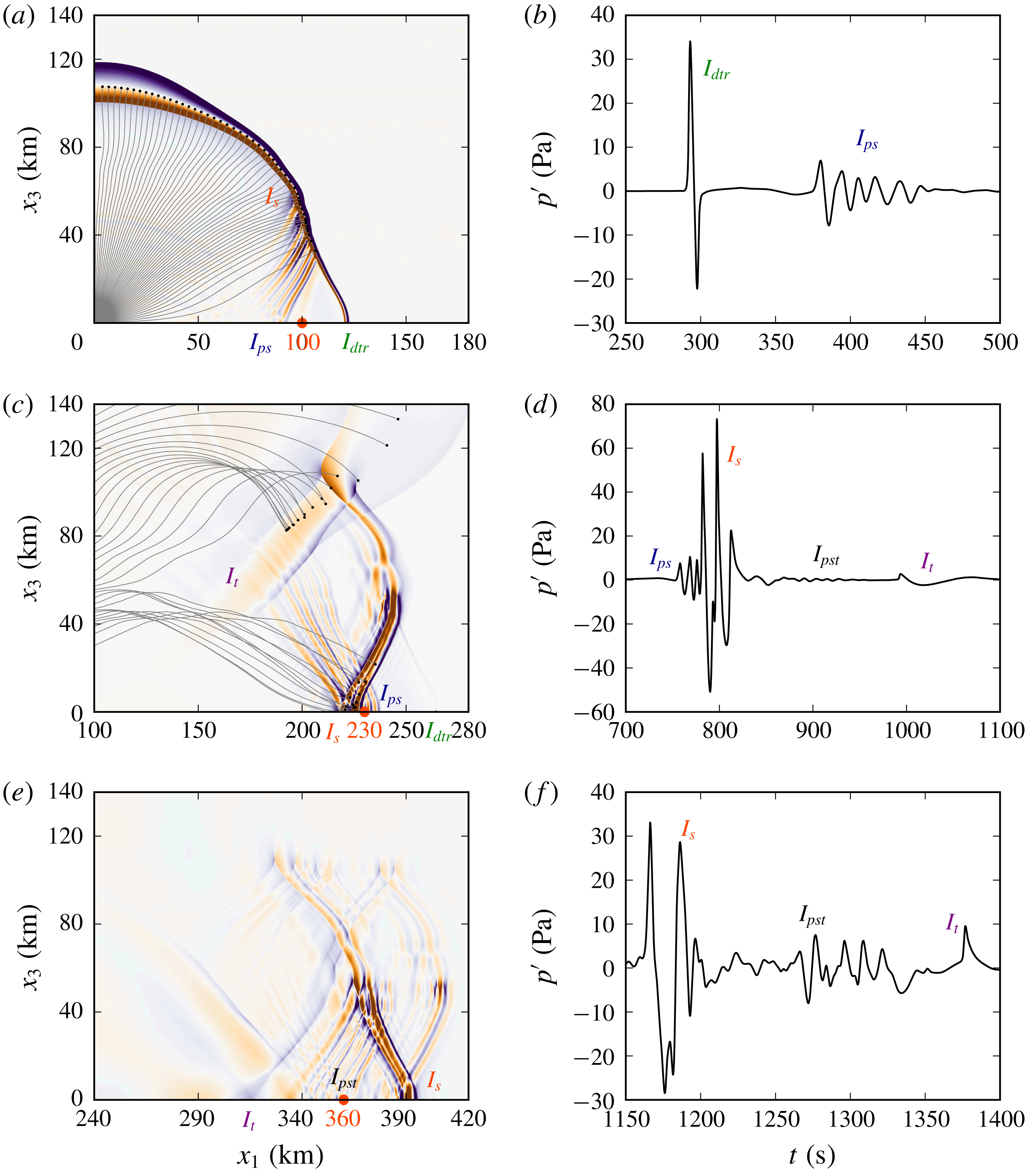
Two waveguides are induced by the vertical profiles (2.1) of the speed of sound and of the wind, a stratospheric duct between the Earth’s surface and about
 $55$
km altitude, and a thermospheric duct between the ground and
 $115$
km altitude. As a consequence, different arrivals reach the Earth’s surface. The pressure perturbations
 $p^{\prime }$
detected on the
 $x_{1}$
axis at the ground stations
 $x_{1}=100$
km,
 $x_{1}=230$
km and
 $x_{1}=360$
km are plotted in figures 12(b), 12(d) and 12(f), respectively. In order to help the understanding of the various arrivals, the acoustic fields
 $\unicode[STIX]{x1D6F7}$
obtained on the
 $x_{1}{-}x_{3}$
plane at times
 $t_{3}$
,
 $t_{5}$
and
 $t_{7}$
are also displayed in figures 12(a), 12(c) and 12(e), respectively. The results obtained by ray theory (Candel Reference Candel1977) are reported as well in figure 12(a,c). At the ground station located at
 $x_{1}=100$
km range, refer to figure 12(b), two distinct wave packets are observed. The first arrival, labelled
 $I_{dtr}$
, where the subscripts
 $d$
and
 $tr$
stand respectively for diffracted and tropospheric, is not predicted by the geometrical acoustics approximation and may be attributed to a creeping wave which diffracts energy along the Earth’s surface (Pierce Reference Pierce1985). It is detected between about
 $t=290$
s and
 $t=300$
s, its maximum overpressure is equal to
 $30.8$
Pa and its duration is around
 $6$
s. No period lengthening is observed, meaning that the propagation at ground level is essentially linear. An analogous conclusion has been drawn in a recent study by de Groot-Hedlin (Reference de Groot-Hedlin2017). The second arrival, detected from
 $t=360$
to
 $460$
s, is associated with the partial reflections the wavefront undergoes while travelling within the small-scale inhomogeneous layer located between
 $25$
and
 $55$
km altitude. For this reason, it is denoted
 $I_{ps}$
, where the subscripts
 $p$
and
 $s$
stand for partial reflection and stratospheric. Its amplitude is about
 $7$
Pa. It can also be remarked that, at time
 $t_{1}$
, a stratospheric return, labelled
 $I_{s}$
, becomes visible in figure 12(a) at about
 $50$
km altitude. At the ground station located at
 $x_{1}=230$
km on the
 $x_{1}$
axis, three different wave packets are recorded along with the partial reflections
 $I_{ps}$
. The stratospheric phase
 $I_{s}$
is observed between
 $780$
and
 $820$
s, with an amplitude equal to about
 $73$
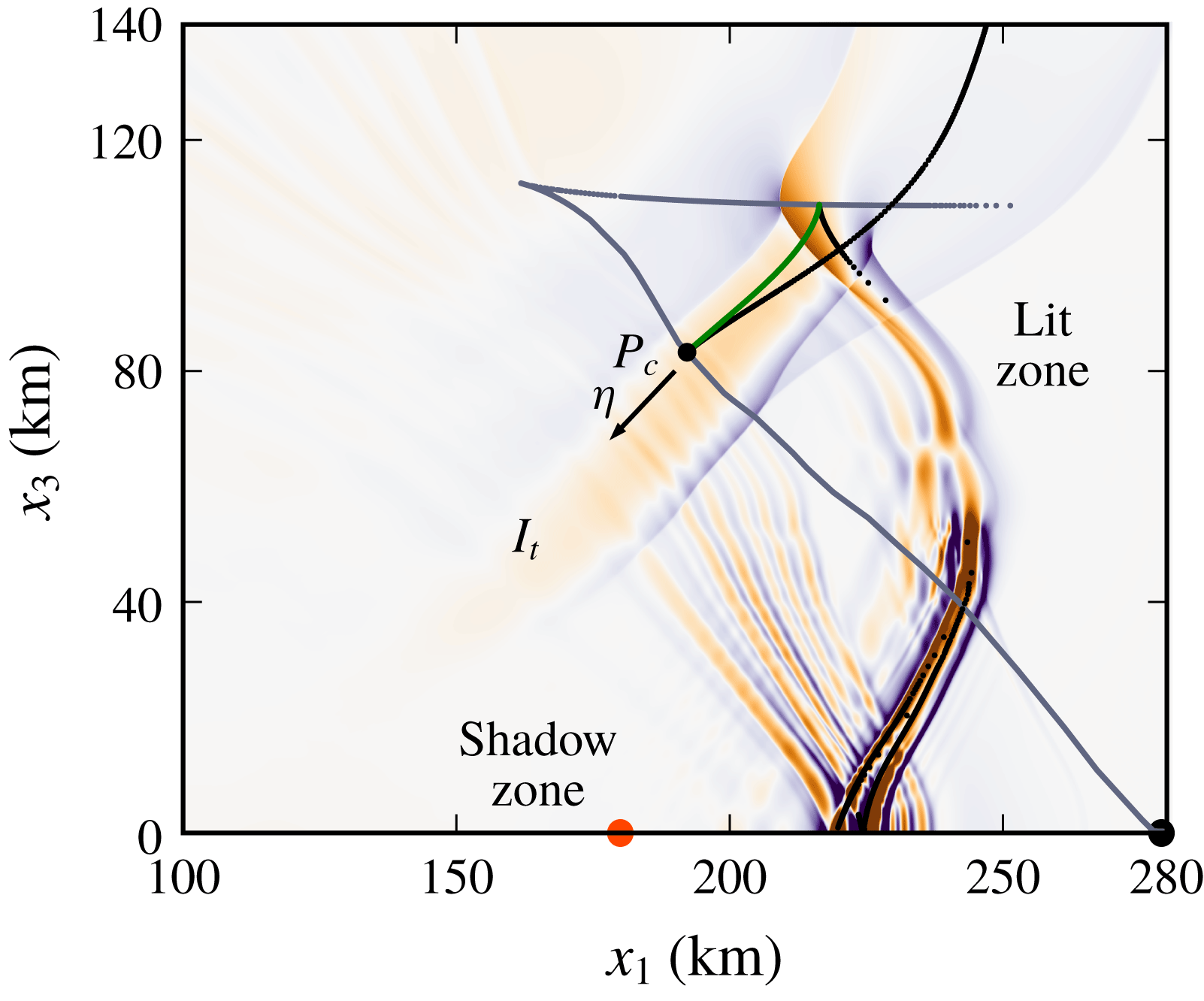
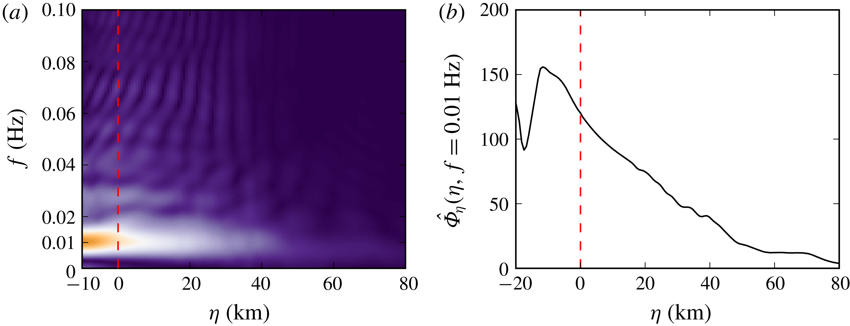
Pa. Furthermore, contrarily to the prediction of ray theory, a thermospheric wave packet
 $I_{t}$
is also detected between
 $980$
and
 $1100$
s, with a maximum overpressure of
 $3$
Pa. As discussed in § 4.7, the arrival
 $I_{t}$
is due to diffraction at the thermospheric caustic. At
 $t=t_{3}$
and
 $t=t_{5}$
, arch-like structures are observed between the ground and the lower thermosphere. They are associated with partial reflections occurring whenever the wavefront propagates downward or upward through the small-scale inhomogeneous layer. The resulting phase, labelled as
 $I_{pst}$
, is clearly visible at the ground stations located at
 $x_{1}=230$
km and at
 $x_{1}=360$
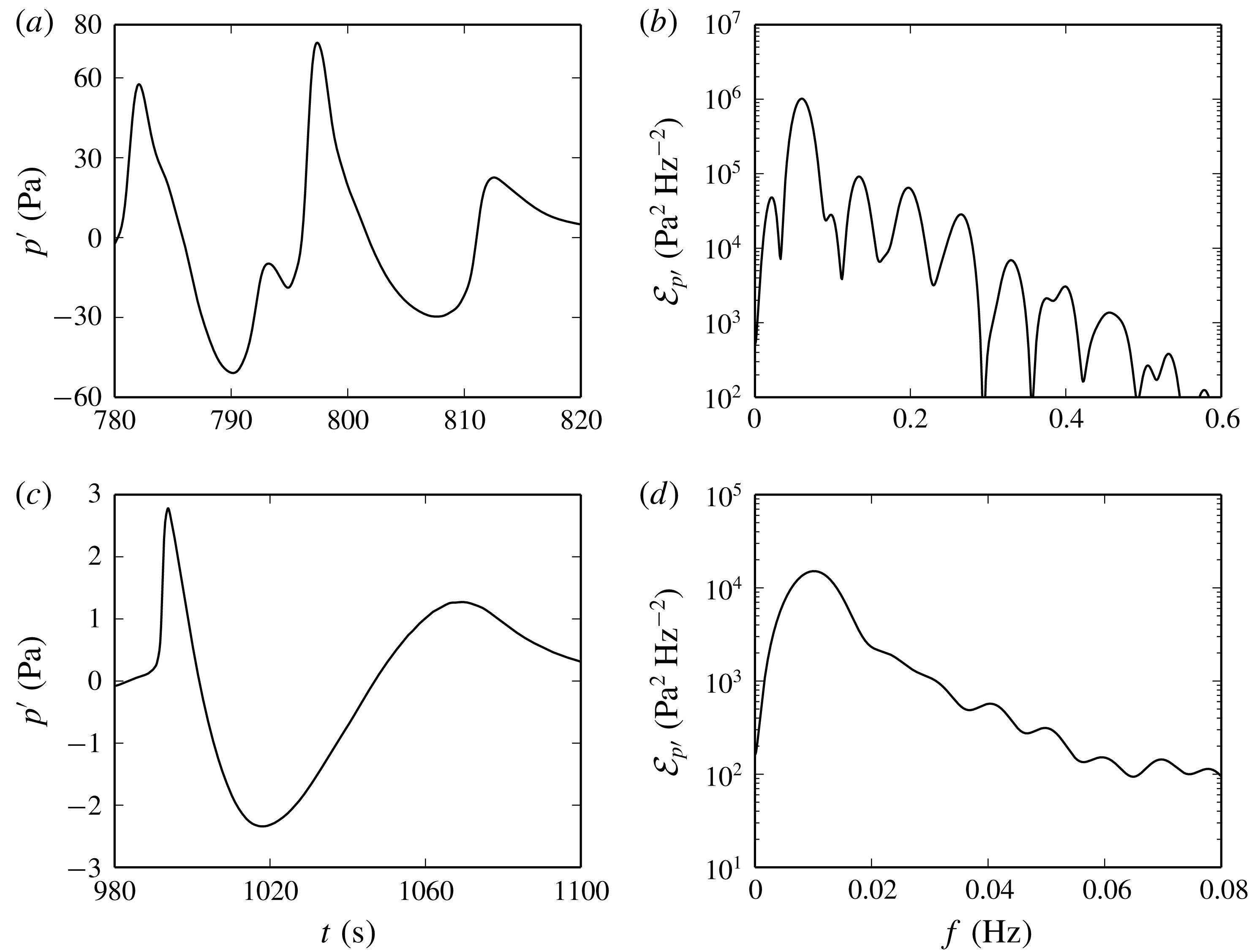
km. Finally, zooms of the stratospheric and thermospheric arrivals detected at
 $x_{1}=230$
km are displayed in figures 13(a) and 13(c), respectively. The corresponding energy spectral densities are reported in figures 13(b) and 13(d). Both signals exhibit U-shaped waveforms. Their durations are around
 $35$
and
 $90$
s, and their central frequencies are equal to about
 $0.06$
and
 $0.01$
Hz.
Zooms of the pressure signals
 $p^{\prime }$
recorded on the
 $x_{1}$
axis at
 $x_{1}=230$
km. (a) Stratospheric and (c) thermospheric arrivals and (b,d) corresponding spectra.

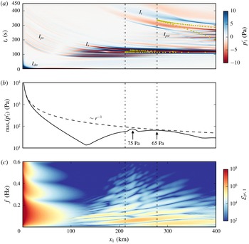
(a) Pressure
 $p_{1}^{\prime }$
recorded at ground level as a function of the distance
 $x_{1}$
and of the retarded time
 $t_{r}$
. Yellow dots are associated with the couples
 $(x_{1},t_{r})$
for which an acoustic ray arrives at the ground. In order to visualize all the infrasonic arrivals, the colour level ranges from
 $-10$
to
 $+10$
Pa. (b) Maximum in time of
 $p_{1}^{\prime }(x_{1},t)$
as a function of the distance
 $x_{1}$
. The dashed line represents the decay of a spherical wave in a free homogeneous medium. (c) Spectrum
 ${\mathcal{E}}_{p^{\prime },1}(x_{1},f)$
of the arrivals recorded at ground level as a function of the distance
 $x_{1}$
and of the frequency
 $f$
.

In order to characterize the different arrivals, the pressure perturbation
 $p_{1}^{\prime }(x_{1},t)=p^{\prime }(x_{1},0,0,t)$
recorded on the
 $x_{1}$
axis is plotted in figure 14(a) as a function of the distance
 $x_{1}$
and of the retarded time
 $t_{r}=t-x_{1}/\bar{c}(0)$
. This diagram allows comparison of the arrival times of the various phases with the one of a wave propagating at ground level with a speed equal to
 $\bar{c}(0)$
. Yellow dots are associated with the couples
 $(x_{1},t_{r})$
for which an acoustic ray is detected. The maximum in time of the function
 $p_{1}^{\prime }$
is illustrated in figure 14(b). The direct phase
 $I_{dtr}$
is recorded without delay, meaning that its propagation speed is close to
 $\bar{c}(0)$
. Its maximum overpressure decreases with range, more rapidly than the amplitude of a spherical wave in a homogeneous medium. As discussed in § 4.5, this decay is associated with the negative gradient of the speed of sound in the troposphere, which deviates the acoustic energy towards the upper atmosphere. The direct phase
 $I_{dtr}$
represents the dominant contribution up to
 $x_{1}=130$
km. The partial reflections
 $I_{ps}$
are detected all along the
 $x_{1}$
axis, with a delay which diminishes with the distance
 $x_{1}$
. The amplitude of
 $I_{ps}$
is of the order of
 $1$
Pa between
 $x_{1}=0$
km and
 $x_{1}=70$
km, reaches a local minimum at
 $x_{1}=70$
km and then increases again up to values of about
 $15$
Pa at
 $x_{1}=140$
km. In addition, a phase jump of
 $\unicode[STIX]{x03C0}$
is observed at
 $x_{1}=70$
km. The stratospheric arrival
 $I_{s}$
is recorded for
 $x_{1}\gtrsim 100$
km, whereas, according to ray theory, it can be detected only for
 $x_{1}\gtrsim 212$
km. The stratospheric phase represents the most important contribution to the pressure signal for
 $x_{1}\gtrsim 120$
km. Its amplitude remains higher than
 $10$
Pa up to at least
 $x_{1}=450$
km, with two local maxima of
 $75$
and
 $65$
Pa at
 $x_{1}=230$
km and
 $x_{1}=275$
km, respectively. The thermospheric phase
 $I_{t}$
is detected at ground level for
 $x_{1}\gtrsim 180$
km, while the geometrical-acoustics approximation predicts no arrival for
 $x_{1}\lesssim 280$
km. The amplitude of the signal
 $I_{t}$
is much lower than the maximum overpressure of the stratospheric wave packet, mainly as a result of the nonlinear lengthening in the upper atmosphere.
The spectrum
 ${\mathcal{E}}_{p^{\prime },1}(x_{1},f)={\mathcal{E}}_{p^{\prime }}(x_{1},0,0,f)$
of the various arrivals recorded at ground level is finally displayed in figure 14(c) as a function of the distance along the
 $x_{1}$
axis and of the frequency
 $f$
. Up to
 $x_{1}=100$
km, the main contribution is due to the direct phase
 $I_{dtr}$
, which has an N-waveform, leading to a broadband spectrum
 ${\mathcal{E}}_{p^{\prime },1}$
. On the contrary, the energy spectral density
 ${\mathcal{E}}_{p^{\prime },1}$
of the arrivals beyond
 $x_{1}=100$
km is essentially contained in the frequency range
 $[0,0.3]\,\text{Hz}$
.
4.5 Analysis of the direct arrival
 $I_{dtr}$

As previously mentioned, the direct arrival
 $I_{dtr}$
is not predicted by the geometrical acoustics. Because of the negative vertical gradient of the speed of sound, rays are deviated towards the upper atmosphere and do not reach the ground up to
 $x_{1}=212$
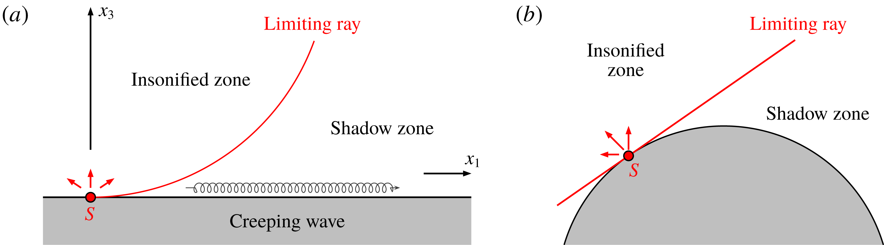
km distance from the source location. From a physical point of view, the effect of an inhomogeneous atmosphere can be better understood with the help of an analogy proposed by Pierce (Reference Pierce1985) and Berry & Daigle (Reference Berry and Daigle1988) among others. The sound field above a flat surface in a quiescent and upward refracting atmosphere, i.e. with a negative vertical gradient of the speed of sound, can be considered equivalent to the acoustic field above a curved convex surface in a homogeneous medium, as illustrated in figure 15. In the latter case, the rays emanating from the source are straight lines and, for geometrical reasons, cannot penetrate into the region below the tangent to the curved ground, which is called shadow zone. Hence, in the shadow side of the sound field, no ray can be detected and, according to the geometrical theory, the amplitude of the pressure perturbation
 $p^{\prime }$
should be nil. The direct arrival
 $I_{dtr}$
is thus induced by diffraction and is interpreted as a creeping wave propagating along the
 $x_{1}$
axis.
Equivalence between (a) the sound field above a flat ground in an upward refracting atmosphere and (b) the acoustic field above a convex surface in a homogeneous medium.

In order to gain more insight into how acoustic energy penetrates in the shadow zone and, in particular, on the Earth’s surface, an analysis of the phase
 $I_{dtr}$
is carried out in this paragraph. As formerly stated, propagation at ground level is essentially linear, excepting in the source region. Furthermore, viscous and thermal conduction effects play a minor role in the troposphere. Besides, to simplify the forthcoming developments, the mean atmosphere is modelled as an effective quiescent medium with the speed of sound and the density given by
 $\bar{c}_{eff}=\bar{c}+\bar{u}_{1}$
and
 $\bar{\unicode[STIX]{x1D70C}}_{eff}=\bar{\unicode[STIX]{x1D70C}}\bar{c}^{2}/\bar{c}_{eff}^{2}$
, respectively. As demonstrated by Godin (Reference Godin2002), such an approximation is valid for low angles of propagation with respect to the horizontal axis, and is consequently justified for a creeping wave. Under the above hypotheses, the acoustic field is axisymmetric and the normalized pressure perturbation
 $\unicode[STIX]{x1D6F7}=p^{\prime }/\sqrt{\bar{\unicode[STIX]{x1D70C}}_{eff}}$
can be described by the wave equation (Bergmann Reference Bergmann1946; Pierce Reference Pierce1990)
 $$\begin{eqnarray}\frac{\unicode[STIX]{x2202}^{2}\unicode[STIX]{x1D6F7}}{\unicode[STIX]{x2202}\unicode[STIX]{x1D71A}^{2}}+\frac{1}{\unicode[STIX]{x1D71A}}\frac{\unicode[STIX]{x2202}\unicode[STIX]{x1D6F7}}{\unicode[STIX]{x2202}\unicode[STIX]{x1D71A}}+\frac{\unicode[STIX]{x2202}^{2}\unicode[STIX]{x1D6F7}}{\unicode[STIX]{x2202}x_{3}^{2}}+\left[\frac{1}{2\bar{\unicode[STIX]{x1D70C}}_{eff}}\frac{\text{d}^{2}\bar{\unicode[STIX]{x1D70C}}_{eff}}{\text{d}x_{3}^{2}}-\frac{3}{4\bar{\unicode[STIX]{x1D70C}}_{eff}^{2}}\left(\frac{\text{d}\bar{\unicode[STIX]{x1D70C}}_{eff}}{\text{d}x_{3}}\right)^{2}\right]\unicode[STIX]{x1D6F7}-\frac{1}{\bar{c}_{eff}^{2}(x_{3})}\frac{\unicode[STIX]{x2202}^{2}\unicode[STIX]{x1D6F7}}{\unicode[STIX]{x2202}t^{2}}=\frac{G}{\sqrt{\bar{\unicode[STIX]{x1D70C}}_{eff}}},\end{eqnarray}$$
where
 $\unicode[STIX]{x1D71A}=\sqrt{x_{1}^{2}+x_{2}^{2}}$
and
 $G$
is a function of the source terms
 $\unicode[STIX]{x1D6EC}_{\unicode[STIX]{x1D70C}}$
and
 $\unicode[STIX]{x1D6EC}_{\unicode[STIX]{x1D70C}e_{t}}$
in (2.3). Since the characteristic acoustic wavelength
 $\unicode[STIX]{x1D706}\simeq 2.6$
km is smaller than the typical length scale for variations of the atmospheric density (
 $\simeq 8.4$
km), the vertical derivatives of the function
 $\bar{\unicode[STIX]{x1D70C}}_{eff}$
are henceforth neglected. Taking the Fourier–Bessel transform
 $$\begin{eqnarray}\hat{\unicode[STIX]{x1D712}}(k_{\unicode[STIX]{x1D71A}},x_{3},\unicode[STIX]{x1D714})=\int _{-\infty }^{+\infty }\int _{0}^{+\infty }\unicode[STIX]{x1D712}(\unicode[STIX]{x1D71A},x_{3},t){\mathcal{J}}_{0}(k_{\unicode[STIX]{x1D71A}}\unicode[STIX]{x1D71A})\text{e}^{+\text{i}\unicode[STIX]{x1D714}t}\unicode[STIX]{x1D71A}\,\text{d}\unicode[STIX]{x1D71A}\,\text{d}t,\end{eqnarray}$$
with
 $\unicode[STIX]{x1D712}=\unicode[STIX]{x1D6F7}$
or
 $\unicode[STIX]{x1D712}=G$
and where
 ${\mathcal{J}}_{0}$
is the zeroth-order Bessel function of the first kind, the depth-separated Helmholtz equation is obtained:
 $$\begin{eqnarray}\frac{\text{d}^{2}\hat{\unicode[STIX]{x1D6F7}}}{\text{d}x_{3}^{2}}+\left(\frac{\unicode[STIX]{x1D714}^{2}}{\bar{c}_{eff}}-k_{\unicode[STIX]{x1D71A}}^{2}\right)\hat{\unicode[STIX]{x1D6F7}}=\frac{{\hat{G}}}{\sqrt{\bar{\unicode[STIX]{x1D70C}}_{eff}}}.\end{eqnarray}$$
The normalized pressure perturbation
 $\unicode[STIX]{x1D6F7}$
is then retrieved by the inverse transform
 $$\begin{eqnarray}\unicode[STIX]{x1D6F7}(\unicode[STIX]{x1D71A},x_{3},t)=\frac{1}{4\unicode[STIX]{x03C0}}\iint _{-\infty }^{+\infty }\unicode[STIX]{x1D6F7}(k_{\unicode[STIX]{x1D71A}},x_{3},\unicode[STIX]{x1D714}){\mathcal{H}}_{0}^{(1)}(k_{\unicode[STIX]{x1D71A}}\unicode[STIX]{x1D71A})\text{e}^{-\text{i}\unicode[STIX]{x1D714}t}k_{\unicode[STIX]{x1D71A}}\,\text{d}k_{\unicode[STIX]{x1D71A}}\,\text{d}\unicode[STIX]{x1D714},\end{eqnarray}$$
where
 ${\mathcal{H}}_{0}^{(1)}$
is the zeroth-order Hankel function of the first kind. By means of the residue theorem, it is possible to demonstrate that integral (4.7) can be approximated by a linear combination of the eigenfunctions
 $\hat{\unicode[STIX]{x1D6F7}}$
of the differential equation (Jensen et al.
Reference Jensen, Kuperman, Porter and Schmidt2011)
 $$\begin{eqnarray}\frac{\text{d}^{2}\hat{\unicode[STIX]{x1D6F7}}}{\text{d}x_{3}^{2}}+\left(\frac{\unicode[STIX]{x1D714}^{2}}{\bar{c}_{eff}}-k_{\unicode[STIX]{x1D71A}}^{2}\right)\hat{\unicode[STIX]{x1D6F7}}=0,\end{eqnarray}$$
completed with the rigid-wall constraint
 $$\begin{eqnarray}\frac{\text{d}\hat{\unicode[STIX]{x1D6F7}}}{\text{d}x_{3}}=0,\quad x_{3}=0~\text{km},\end{eqnarray}$$
and with the radiation condition
 $$\begin{eqnarray}\hat{\unicode[STIX]{x1D6F7}}\sim \text{e}^{\text{i}k_{3}^{\infty }x_{3}},\quad k_{3}^{\infty }=\lim _{x_{3}\rightarrow +\infty }\sqrt{\frac{\unicode[STIX]{x1D714}^{2}}{\bar{c}_{eff}(x_{3})}-k_{\unicode[STIX]{x1D71A}}^{2}},\quad x_{3}\rightarrow +\infty .\end{eqnarray}$$
The real part of the wavenumber
 $k_{3}^{\infty }$
is required to be positive or nil in order for the function
 $\hat{\unicode[STIX]{x1D6F7}}$
to represent an outgoing wave as
 $x_{3}\rightarrow +\infty$
. Since the diffracted arrival
 $I_{dtr}$
is mainly influenced by the negative gradient of the temperature in the troposphere, the function
 $\bar{c}_{eff}$
is here defined as
 $$\begin{eqnarray}\bar{c}_{eff}(x_{3})=\left\{\begin{array}{@{}ll@{}}\bar{c}(x_{3})+\bar{u}_{1}(x_{3}),\quad & x_{3}\in [0,x_{3}^{\infty }]\\ \bar{c}(x_{3}^{\infty })+\bar{u}_{1}(x_{3}^{\infty }),\quad & x_{3}>x_{3}^{\infty },\end{array}\right.\end{eqnarray}$$
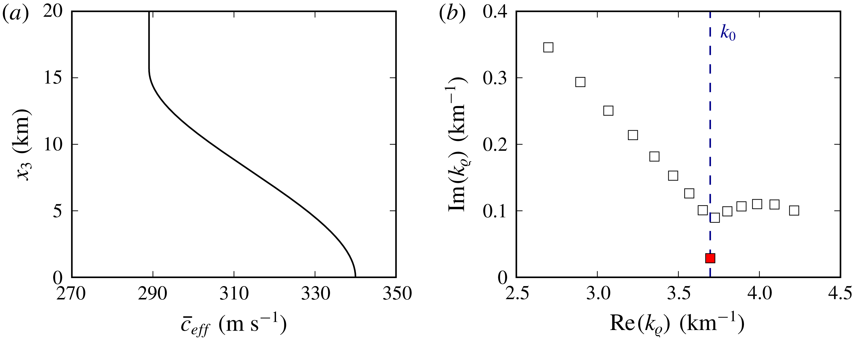
(a) Effective speed of sound profile
 $\bar{c}_{eff}$
. (b) Wavenumbers
 $k_{\unicode[STIX]{x1D71A}}$
for
 $f=0.2$
Hz; the red square corresponds to the least attenuated mode.

where
 $x_{3}^{\infty }=15.75$
km is the altitude of the first minimum of the sum
 $\bar{c}(x_{3})+\bar{u}_{1}(x_{3})$
. The resulting profile
 $\bar{c}_{eff}(x_{3})$
is displayed in figure 16(a). In line with this definition, the above radiation condition is replaced by the following boundary constraint (Jensen et al.
Reference Jensen, Kuperman, Porter and Schmidt2011):
 $$\begin{eqnarray}\frac{\text{d}\hat{\unicode[STIX]{x1D6F7}}}{\text{d}x_{3}}-\text{i}k_{3}^{\infty }\hat{\unicode[STIX]{x1D6F7}}=0,\quad k_{3}^{\infty }=\sqrt{\frac{\unicode[STIX]{x1D714}^{2}}{\bar{c}_{eff}(x_{3}^{\infty })}-k_{\unicode[STIX]{x1D71A}}^{2}},\quad x_{3}=x_{3}^{\infty }.\end{eqnarray}$$
Problem (4.8) represents a differential eigensystem and can be solved through a pseudospectral collocation method (Bertin et al.
Reference Bertin, Millet and Bouche2014; Sabatini & Bailly Reference Sabatini and Bailly2015). As an illustration, the eigenvalues
 $k_{\unicode[STIX]{x1D71A}}$
obtained for
 $f=0.2$
Hz are plotted in figure 16(b). As suggested by Pierce (Reference Pierce1985), along the
 $x_{1}$
axis, integral (4.7) is dominated by wavenumbers
 $k_{\unicode[STIX]{x1D71A}}$
close to
 $k_{0}=\unicode[STIX]{x1D714}/\bar{c}_{eff}(0)$
. Moreover, since the imaginary parts of the eigenvalues
 $k_{\unicode[STIX]{x1D71A}}$
are strictly positive, the corresponding contributions, which are proportional to
 ${\mathcal{H}}_{0}^{(1)}(k_{\unicode[STIX]{x1D71A}}r)$
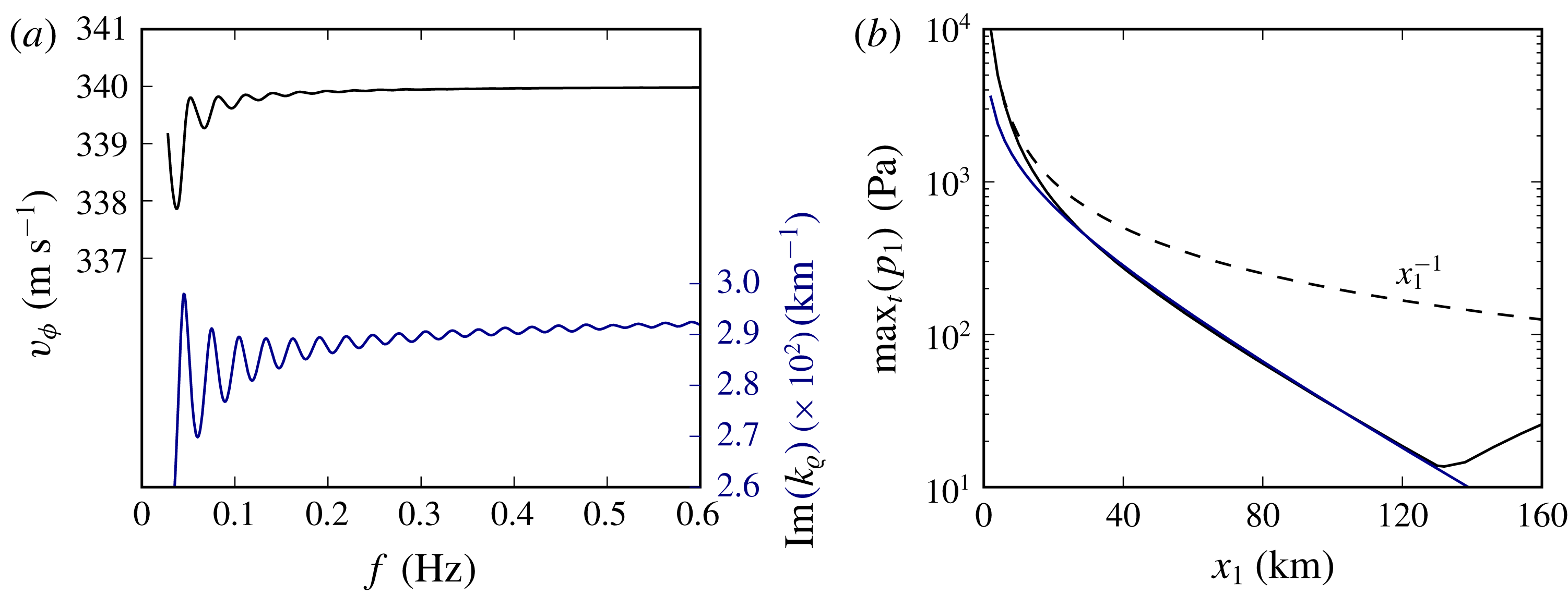
, decay with distance. Consequently, at large distances, only the least attenuated mode is likely to be observed. The phase speed
 $v_{\unicode[STIX]{x1D719}}=\unicode[STIX]{x1D714}/\text{Re}(k_{\unicode[STIX]{x1D71A}})$
and the imaginary part
 $\unicode[STIX]{x1D6FC}=\min _{k_{\unicode[STIX]{x1D71A}}}(\text{Im}(k_{\unicode[STIX]{x1D71A}}))$
of the least attenuated mode are depicted as functions of the frequency
 $f$
in figure 17(a). Globally, they both depend weakly on the pulsation
 $\unicode[STIX]{x1D714}$
. For
 $f>0.05$
Hz, the velocity
 $v_{\unicode[STIX]{x1D719}}$
is approximately equal to
 $\bar{c}_{eff}(0)=340~\text{m}~\text{s}^{-1}$
, and the attenuation factor
 $\unicode[STIX]{x1D6FC}$
increases only slightly as
 $f$
augments and has an average value of about
 $\unicode[STIX]{x1D6FC}_{mean}=2.85\times 10^{-2}~\text{km}^{-1}$
in the range
 $[0.05,0.2]$
Hz. As the wind velocity is nil at ground level, the least attenuated mode propagates with a celerity equal to the speed of sound on the Earth’s surface,
 $\bar{c}(0)$
, which confirms the result of the previous paragraph. Moreover, by virtue of the above considerations, the absolute value of the pressure perturbation
 $p^{\prime }$
along the
 $x_{1}$
axis and in the far range is found to behave as
 $$\begin{eqnarray}p^{\prime }(x_{1},0,0,t)\propto \frac{1}{\sqrt{x_{1}}}\text{e}^{-\unicode[STIX]{x1D6FC}_{mean}x_{1}},\end{eqnarray}$$
since
 ${\mathcal{H}}_{0}^{(1)}(k_{\unicode[STIX]{x1D71A}}x_{1})\sim 1/\sqrt{x_{1}}$
for
 $k_{\unicode[STIX]{x1D71A}}x_{1}\gg 1$
. Hence, conforming to earlier remarks, the amplitude of the phase
 $I_{dtr}$
weakens more rapidly than that of a spherical wave in a homogeneous medium, for which
 $p^{\prime }(x_{1},0,0,t)\propto 1/x_{1}$
. To conclude, the maximum in time of the function
 $p_{1}^{\prime }$
is again illustrated in figure 17(b) and compared to the result given by expression (4.9). A very good agreement is observed between numerical and theoretical predictions for
 $x_{1}>20$
km.
(a) Phase speed (black line) and imaginary part (blue line) of the least attenuated mode. (b) Maximum in time of the function
 $p_{1}^{\prime }(x_{1},t)$
as a function of the distance
 $x_{1}$
, compared to the result given by formula (4.9) and to the behaviour of a spherical wave in a homogeneous medium.

4.6 Analysis of the partial reflections
The sensitivity of ground recordings to the speed of sound and wind fluctuations of length scale of the same order as the acoustic wavelength has received particular attention in recent years (Chunchuzov et al.
Reference Chunchuzov, Kulichkov, Popov, Waxler and Assink2011, Reference Chunchuzov, Kulichkov, Popov and Hedlin2014, Reference Chunchuzov, Kulichkov, Popov, Perepelkin, Vasilev, Glushkov and Firstov2015; Bertin et al.
Reference Bertin, Millet and Bouche2014). In particular, Chunchuzov et al. (Reference Chunchuzov, Kulichkov, Popov and Hedlin2014, Reference Chunchuzov, Kulichkov, Popov, Perepelkin, Vasilev, Glushkov and Firstov2015) demonstrated the feasibility of retrieving the vertical structure of the atmosphere from the reflected signals, whose energy spectral densities are closely related to the characteristic wavenumbers of the inhomogeneities. In order to gain more insight into the relationship between the wavenumber spectrum of the atmospheric fluctuations and the Fourier transform of the partial reflections, a more detailed analysis of the phase
 $I_{ps}$
is now carried out on a simplified model.
4.6.1 Reflection of a spherical wave by a one-dimensional speed-of-sound inhomogeneity
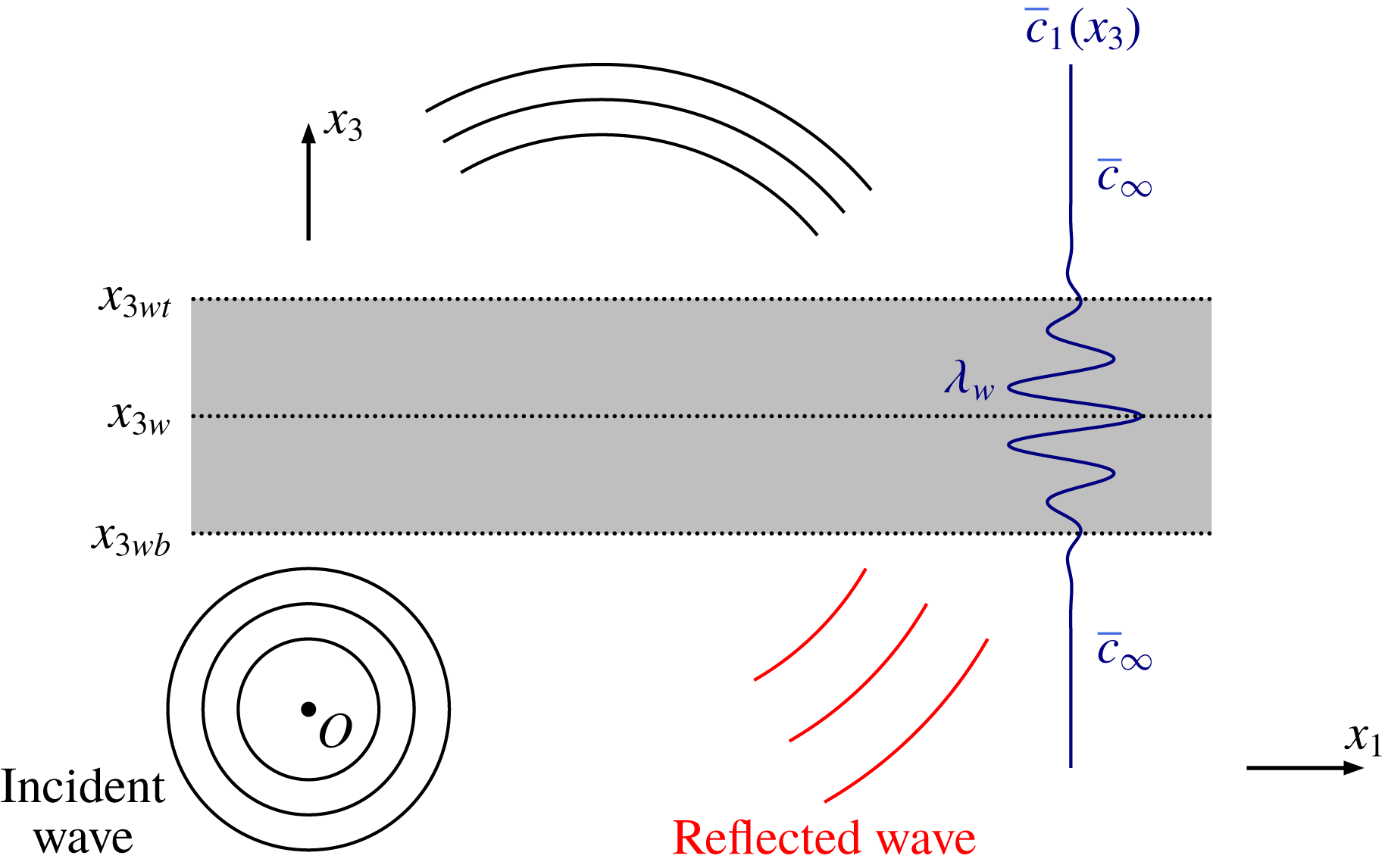
The configuration schematically illustrated in figure 18 is considered. A spherical wavefront is emitted in an infinite domain
 $Ox_{1}x_{2}x_{3}$
by a point source placed at the origin
 $O$
and propagates through a one-dimensional speed-of-sound inhomogeneity confined between the altitudes
 $x_{3wb}$
and
 $x_{3wt}$
; the medium is at rest and the speed of sound away from the inhomogeneity is equal to
 $\bar{c}_{\infty }$
. The interaction between the wavefront and the speed-of-sound fluctuation generates a transmitted wave and a reflected wave. In order to simplify the analytical developments, nonlinear, viscous and thermal conduction effects are henceforth neglected. Moreover, since the large-scale variations of the atmospheric medium induced by the gravitational acceleration do not contribute to the reflected wave, the gradient
 $\text{d}\bar{p}/\text{d}x_{3}$
is assumed nil and the ambient pressure
 $\bar{p}$
is set equal to
 $\bar{p}_{0}$
. Under these hypotheses, the pressure perturbation
 $p^{\prime }$
is described by the wave equation (Bergmann Reference Bergmann1946; Pierce Reference Pierce1990)
 $$\begin{eqnarray}\frac{\unicode[STIX]{x2202}^{2}p^{\prime }}{\unicode[STIX]{x2202}x_{1}^{2}}+\frac{\unicode[STIX]{x2202}^{2}p^{\prime }}{\unicode[STIX]{x2202}x_{2}^{2}}+\bar{\unicode[STIX]{x1D70C}}(x_{3})\frac{\unicode[STIX]{x2202}}{\unicode[STIX]{x2202}x_{3}}\left(\frac{1}{\unicode[STIX]{x1D70C}(x_{3})}\frac{\unicode[STIX]{x2202}p^{\prime }}{\unicode[STIX]{x2202}x_{3}}\right)-\frac{1}{\bar{c}^{2}(x_{3})}\frac{\unicode[STIX]{x2202}^{2}p^{\prime }}{\unicode[STIX]{x2202}t^{2}}=-F(t)\unicode[STIX]{x1D6FF}(\boldsymbol{x}),\end{eqnarray}$$
Propagation of a spherical wave through a small-scale speed-of-sound inhomogeneity.

where
 $F(t)$
indicates the temporal envelope of the point source and
 $\bar{\unicode[STIX]{x1D70C}}(x_{3})=\unicode[STIX]{x1D6FE}\bar{p}_{0}/\bar{c}^{2}(x_{3})$
. As shown in appendix B, for
 $x_{3}\ll x_{3w}$
, the incident sound field
 $p_{i}^{\prime }(\boldsymbol{x},t)$
is represented by
 $$\begin{eqnarray}p_{i}^{\prime }(\boldsymbol{x},t)=\frac{F(t-\Vert \boldsymbol{x}\Vert /\bar{c}_{\infty })}{4\unicode[STIX]{x03C0}\Vert \boldsymbol{x}\Vert }.\end{eqnarray}$$
Accordingly, the temporal shape of the source is advected in space at the speed
 $\bar{c}_{\infty }$
and the maximum overpressure decays as
 $1/\Vert \boldsymbol{x}\Vert$
. Moreover, the temporal Fourier transform
 $\hat{p}_{r}^{\prime }(\boldsymbol{x},\unicode[STIX]{x1D714})$
of the reflected wave
 $p_{r}^{\prime }(\boldsymbol{x},t)$
,
 $$\begin{eqnarray}\hat{p}_{r}^{\prime }(\boldsymbol{x},\unicode[STIX]{x1D714})=\int _{-\infty }^{+\infty }p_{r}^{\prime }(\boldsymbol{x},t)\text{e}^{\text{i}\unicode[STIX]{x1D714}t}\,\text{d}t,\end{eqnarray}$$
is given by the integral
 $$\begin{eqnarray}\hat{p}_{r}^{\prime }(\boldsymbol{x},\unicode[STIX]{x1D714})=\frac{\hat{F}(\unicode[STIX]{x1D714})}{4\unicode[STIX]{x03C0}}\iint _{-\infty }^{+\infty }{\displaystyle \frac{\text{i}{\mathcal{R}}_{c}\text{e}^{+\text{i}[k_{1}x_{1}+k_{2}x_{2}-k_{3}(k_{1},k_{2},\unicode[STIX]{x1D714})x_{3}]}}{2\unicode[STIX]{x03C0}k_{3}(k_{1},k_{2},\unicode[STIX]{x1D714})}}\,\text{d}k_{1}\,\text{d}k_{2},\end{eqnarray}$$
where
 $k_{1}$
,
 $k_{2}$
and
 $k_{3}=\sqrt{(\unicode[STIX]{x1D714}/\bar{c}_{\infty })^{2}-(k_{1}^{2}+k_{2}^{2})}$
represent the wavenumber components,
 $\hat{F}$
is the Fourier transform of
 $F(t)$
and
 ${\mathcal{R}}_{c}$
is the reflection coefficient of the inhomogeneous layer. The acoustic field
 $\hat{p}_{r}^{\prime }$
can be interpreted as a sum of monochromatic plane waves whose amplitude is proportional to both the incident spectrum
 $\hat{F}$
and the reflection coefficient
 ${\mathcal{R}}_{c}$
. The value of
 ${\mathcal{R}}_{c}$
depends on the speed of sound
 $\bar{c}(x_{3})$
, on the incidence angle
 $\unicode[STIX]{x1D711}=\text{atan}(k_{3}/\sqrt{k_{1}^{2}+k_{2}^{2}})$
with respect to the horizontal plane and on the pulsation
 $\unicode[STIX]{x1D714}$
. According to Lekner (Reference Lekner1987), the reflection coefficient
 ${\mathcal{R}}_{c}$
is defined as the limit
 $$\begin{eqnarray}{\mathcal{R}}_{c}\equiv \lim _{x_{3}\rightarrow -\infty }r_{c}(x_{3})\text{e}^{2\text{i}\tilde{k}_{3}(x_{3})x_{3}},\end{eqnarray}$$
where the wavenumber
 $\tilde{k}_{3}$
is given by
 $$\begin{eqnarray}\tilde{k}_{3}^{2}(x_{3})\equiv \frac{\unicode[STIX]{x1D714}^{2}}{\bar{c}^{2}(x_{3})}-k_{1}^{2}-k_{2}^{2}=\frac{\unicode[STIX]{x1D714}^{2}}{\bar{c}^{2}(x_{3})}-\frac{\unicode[STIX]{x1D714}^{2}}{\bar{c}_{\infty }^{2}}\cos ^{2}(\unicode[STIX]{x1D711}),\end{eqnarray}$$
and the function
 $r_{c}(x_{3})$
satisfies the Riccati problem
 $$\begin{eqnarray}\frac{\text{d}r_{c}}{\text{d}x_{3}}+2\text{i}\tilde{k}_{3}r_{c}-\frac{\bar{\unicode[STIX]{x1D70C}}}{2\tilde{k_{3}}}\frac{\text{d}(\tilde{k}_{3}/\bar{\unicode[STIX]{x1D70C}})}{\text{d}x_{3}}(1-r_{c}^{2})=0,\end{eqnarray}$$
with the condition
 $$\begin{eqnarray}\lim _{x_{3}\rightarrow +\infty }r_{c}=0.\end{eqnarray}$$
Since the inhomogeneous layer is assumed confined in the interval
 $[x_{3wb},x_{3wt}]$
,
 $r_{c}(x_{3}^{\infty })=0$
for
 $x_{3}^{\infty }>x_{3wt}$
and the above equation can be integrated from
 $x_{3}=x_{3}^{\infty }$
to
 $x_{3}=x_{3}^{-\infty }<x_{3wb}$
through any stable time-integration algorithm.
4.6.2 Reflection coefficient of a Morlet wavelet
The reflection coefficient is now analysed for a speed of sound
 $\bar{c}(x_{3})$
defined as the sum of a constant
 $\bar{c}_{\infty }$
and an elementary Morlet wavelet of amplitude
 $\unicode[STIX]{x1D716}_{\bar{c}}\bar{c}_{\infty }$
, of wavelength
 $\unicode[STIX]{x1D706}_{w}$
and located at altitude
 $x_{3w}$
:
 $$\begin{eqnarray}\bar{c}(x_{3})=\bar{c}_{\infty }[1+\unicode[STIX]{x1D716}_{\bar{c}}\text{e}^{-z^{2}/2}\cos (2\unicode[STIX]{x03C0}z)],\quad \text{with}~z=\frac{x_{3}-x_{3w}}{\unicode[STIX]{x1D706}_{w}}.\end{eqnarray}$$
Hereafter, the parameter
 $\unicode[STIX]{x1D716}_{\bar{c}}$
will be considered small. The modulus
 $|{\mathcal{R}}_{c}|$
obtained with
 $\unicode[STIX]{x1D716}_{\bar{c}}\bar{c}_{\infty }=5~\text{m}~\text{s}^{-1}$
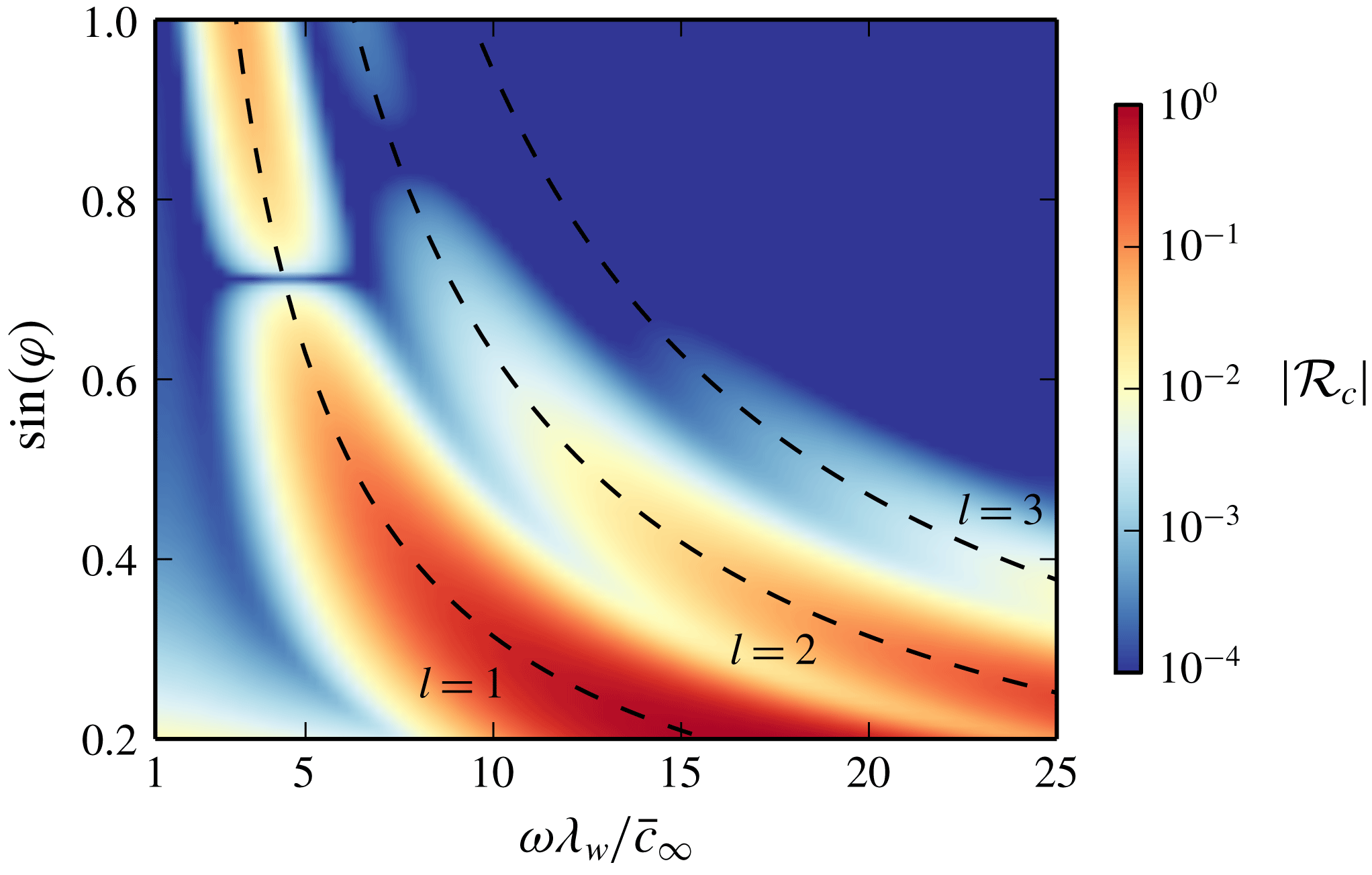
is plotted in figure 19 as a function of the normalized pulsation
 $\unicode[STIX]{x1D714}\unicode[STIX]{x1D706}_{w}/\bar{c}_{\infty }$
and of the sinus of the incidence angle
 $\unicode[STIX]{x1D711}$
. The function
 $|{\mathcal{R}}_{c}|$
is different from zero only in specific frequency bands and its maxima approximately satisfy the well-known Bragg law (Blanc-Benon, Dallois & Juvé Reference Blanc-Benon, Dallois and Juvé2001)
 $$\begin{eqnarray}2\unicode[STIX]{x1D706}_{w}\sin (\unicode[STIX]{x1D711})=l\unicode[STIX]{x1D706},\end{eqnarray}$$
where
 $l$
is an integer number and
 $\unicode[STIX]{x1D706}=2\unicode[STIX]{x03C0}\bar{c}_{\infty }/\unicode[STIX]{x1D714}$
is the incident wavelength. The modulus
 $|{\mathcal{R}}_{c}|$
increases as
 $\unicode[STIX]{x1D711}$
tends to
 $0$
, and is close to
 $1$
for incidences
 $\unicode[STIX]{x1D711}$
lower than about
 $10^{\circ }$
. In this case, the associated plane wave is totally reflected. Moreover, in each frequency band, there exists an angle
 $\unicode[STIX]{x1D711}_{t}$
, called intromission angle, for which
 ${\mathcal{R}}_{c}$
is nil and the signal is totally transmitted. As an example,
 $\unicode[STIX]{x1D711}_{t}$
is equal to
 $45^{\circ }$
for
 $l=1$
and to about
 $57.3^{\circ }$
for
 $l=2$
.
Reflection coefficient
 ${\mathcal{R}}_{c}$
for the speed of sound profile (4.18) as a function of the normalized pulsation
 $\unicode[STIX]{x1D714}\unicode[STIX]{x1D706}_{w}\bar{c}_{\infty }$
and of the sinus of the incidence angle
 $\sin (\unicode[STIX]{x1D711})$
. The dashed lines represent the well-known Bragg law
 $2\unicode[STIX]{x1D706}_{w}\sin (\unicode[STIX]{x1D711})=l\unicode[STIX]{x1D706}$
, for
 $l=1$
,
 $l=2$
and
 $l=3$
.

According to Lekner (Reference Lekner1987), under the hypothesis of weak reflection, a first approximation of the function
 ${\mathcal{R}}_{c}$
for a generic inhomogeneity
 $\bar{c}^{\prime }=\bar{c}-\bar{c}_{\infty }$
is given by the integral
 $$\begin{eqnarray}{\mathcal{R}}_{c}\simeq \int _{-\infty }^{+\infty }\left[\frac{\text{i}\unicode[STIX]{x0394}\tilde{k}_{3}^{2}}{2k_{3}}+\frac{1}{2}\frac{1}{\bar{\unicode[STIX]{x1D70C}}}\frac{\text{d}\bar{\unicode[STIX]{x1D70C}}}{\text{d}x_{3}}\right]\text{e}^{2\text{i}k_{3}x_{3}}\,\text{d}x_{3},\quad \text{with}~\unicode[STIX]{x0394}\tilde{k}_{3}^{2}(x_{3})=\frac{\unicode[STIX]{x1D714}^{2}}{\bar{c}^{2}(x_{3})}-\frac{\unicode[STIX]{x1D714}^{2}}{\bar{c}_{\infty }^{2}}.\end{eqnarray}$$
For weak inhomogeneities (
 $\bar{c}^{\prime }/\bar{c}_{\infty }\ll 1$
), the density gradient can be rewritten as
 $(\text{d}\bar{\unicode[STIX]{x1D70C}}/\text{d}x_{3})/\bar{\unicode[STIX]{x1D70C}}=-2(\text{d}\bar{c}^{\prime }/\text{d}x_{3})/\bar{c}_{\infty }$
. As a result, integral (4.20) can be further simplified as
 $$\begin{eqnarray}{\mathcal{R}}_{c}\simeq \text{i}\frac{1}{k_{3}}\frac{\unicode[STIX]{x1D714}^{2}}{\bar{c}_{\infty }^{2}}(2\sin ^{2}(\unicode[STIX]{x1D711})-1)\int _{-\infty }^{+\infty }\frac{\bar{c}^{\prime }(x_{3})}{\bar{c}_{\infty }}\text{e}^{2\text{i}k_{3}x_{3}}\,\text{d}x_{3}.\end{eqnarray}$$
This formula allows relating the reflection coefficient
 ${\mathcal{R}}_{c}$
to the spectrum of the speed of sound fluctuations;
 ${\mathcal{R}}_{c}$
is indeed proportional to the Fourier transform of the inhomogeneity
 $\bar{c}^{\prime }/\bar{c}_{\infty }$
. Furthermore, because of the factor
 $(2\sin ^{2}(\unicode[STIX]{x1D711})-1)$
, the function
 ${\mathcal{R}}_{c}$
vanishes for
 $\unicode[STIX]{x1D711}=\unicode[STIX]{x1D711}_{t}=45^{\circ }$
. Hence, the existence of an intromission angle
 $\unicode[STIX]{x1D711}_{t}$
is not peculiar to the profile (4.18) and is strictly linked to the density variations
 $(\text{d}\bar{\unicode[STIX]{x1D70C}}/\text{d}x_{3})/\bar{\unicode[STIX]{x1D70C}}$
, which, under the assumption
 $\text{d}\bar{p}/\text{d}x_{3}=0$
, are only induced by the gradient of the speed of sound
 $\text{d}\bar{c}^{\prime }/\text{d}x_{3}$
. For
 $\unicode[STIX]{x1D711}=\unicode[STIX]{x1D711}_{t}$
, the effect of the fluctuations of
 $\bar{\unicode[STIX]{x1D70C}}$
is exactly compensated by the effect of the speed-of-sound inhomogeneity.
To conclude, for the specific case of the profile (4.18), it can be shown that the reflection coefficient
 ${\mathcal{R}}_{c}$
can be written as
 ${\mathcal{R}}_{c}\equiv {\mathcal{R}}\text{e}^{2\text{i}k_{3}\unicode[STIX]{x1D706}_{w}}$
, where the auxiliary function
 ${\mathcal{R}}$
is approximately equal to
 $$\begin{eqnarray}{\mathcal{R}}\simeq \text{i}\frac{\sqrt{2\unicode[STIX]{x03C0}}\,\unicode[STIX]{x1D716}_{\bar{c}}}{k_{3}\unicode[STIX]{x1D706}_{w}}\frac{\unicode[STIX]{x1D714}^{2}\unicode[STIX]{x1D706}_{w}^{2}}{\bar{c}_{\infty }^{2}}(2\sin ^{2}(\unicode[STIX]{x1D711})-1)\text{e}^{-2k_{3}^{2}\unicode[STIX]{x1D706}_{w}^{2}-2\unicode[STIX]{x03C0}^{2}}\cosh (4\unicode[STIX]{x03C0}k_{3}\unicode[STIX]{x1D706}_{w}).\end{eqnarray}$$
This function takes pure imaginary values and exhibits a jump of
 $\unicode[STIX]{x03C0}$
at the intromission angle
 $\unicode[STIX]{x1D711}=\unicode[STIX]{x1D711}_{t}$
. Moreover, the modulus
 $|{\mathcal{R}}_{c}|=|{\mathcal{R}}|$
increases linearly with the amplitude of the speed-of-sound inhomogeneity.
4.6.3 Amplitude of the wave reflected by a Morlet wavelet along the
$x_{1}$
axis

By using the auxiliary variable
 ${\mathcal{R}}$
, the reflected sound field (4.13) can be recast as follows:
 $$\begin{eqnarray}\hat{p}_{r}^{\prime }(\boldsymbol{x},\unicode[STIX]{x1D714})=\frac{\hat{F}(\unicode[STIX]{x1D714})}{4\unicode[STIX]{x03C0}}\iint _{-\infty }^{+\infty }{\displaystyle \frac{\text{i}{\mathcal{R}}\text{e}^{+\text{i}[k_{1}x_{1}+k_{2}x_{2}-k_{3}(k_{1},k_{2},\unicode[STIX]{x1D714})(x_{3}-2x_{3w})]}}{2\unicode[STIX]{x03C0}k_{3}(k_{1},k_{2},\unicode[STIX]{x1D714})}}\,\text{d}k_{1}\,\text{d}k_{2}.\end{eqnarray}$$
This integral can be drastically simplified through the method of the stationary phase (Frisk Reference Frisk1994). More specifically, with reference to figure 20, it can be shown that, at a given recording station
 $S_{R}$
, the function
 $\hat{p}_{r}^{\prime }(\boldsymbol{x},\unicode[STIX]{x1D714})$
can be approximated as
 $$\begin{eqnarray}\hat{p}_{r}^{\prime }(\boldsymbol{x},\unicode[STIX]{x1D714})\simeq \hat{F}(\unicode[STIX]{x1D714}){\mathcal{R}}(\unicode[STIX]{x1D711}_{st},\unicode[STIX]{x1D714})\frac{\text{e}^{-\text{i}\unicode[STIX]{x1D714}r_{\star }/\bar{c}_{\infty }}}{4\unicode[STIX]{x03C0}r_{\star }},\end{eqnarray}$$
where
 $\unicode[STIX]{x1D711}_{st}=\text{atan}(x_{3w}/(\sqrt{x_{1}^{2}+x_{2}^{2}}/2))$
and
 $r_{\star }=\Vert \overrightarrow{O^{\prime }S_{R}}\Vert$
. The variable
 $\unicode[STIX]{x1D711}_{st}$
represents the angle formed with the horizontal plane by the line connecting the source
 $O$
with the intersection point between the incident wavefront and the symmetry axis
 $x_{3}=x_{3w}$
of the speed-of-sound profile; the term
 $r_{\star }$
is the distance between the point
 $O^{\prime }$
, located at the altitude
 $x_{3}=2x_{3w}$
, and the recording station
 $S_{R}$
. From a physical point of view, equation (4.24) states that the reflected field
 $\hat{p}_{r}^{\prime }$
consists of a spherical wave emanating from the image source
 $O^{\prime }$
, whose amplitude is proportional to the incident spectrum
 $\hat{F}(\unicode[STIX]{x1D714})$
and to the reflection coefficient
 ${\mathcal{R}}$
for a plane wave having an incidence angle equal to the specular angle
 $\unicode[STIX]{x1D711}=\unicode[STIX]{x1D711}_{st}$
. Expression (4.24) represents the geometrical approximation of the reflected field, according to which the reflected energy is mainly concentrated in the direction of the specular angle. The modulus
 $|\hat{p}_{r}^{\prime }|$
is finally given by the relation
 $$\begin{eqnarray}|\hat{p}_{r}^{\prime }(\boldsymbol{x},\unicode[STIX]{x1D714})|\simeq \left|\frac{\hat{F}(\unicode[STIX]{x1D714}){\mathcal{R}}(\unicode[STIX]{x1D711}_{st},\unicode[STIX]{x1D714})}{4\unicode[STIX]{x03C0}r_{\star }}\right|.\end{eqnarray}$$
Since the reflection coefficient
 $|{\mathcal{R}}|$
is different from zero only in particular frequency bands, the above formula states that the inhomogeneous layer acts as a selective filter which reflects only specific wavelengths of the incident spectrum.
Propagation of a spherical wave through a small-scale inhomogeneity. At the receiver
 $S_{R}$
, the main contribution to the reflected wave comes from the specular angle
 $\unicode[STIX]{x1D711}_{st}$
, formed with the
 $x_{1}$
axis by the ray connecting the point source
 $O$
and the intersection between the incident spherical wave and the symmetry axis of the inhomogeneity.

4.6.4 Reflection coefficient of a wind inhomogeneity
The above results, obtained for a small-scale speed-of-sound inhomogeneity, cannot be readily extended to the case of wind fluctuations. However, two-dimensional simulations carried out by the authors suggest that, for incidences
 $\unicode[STIX]{x1D711}$
lower than the intromission angle
 $\unicode[STIX]{x1D711}_{t}$
and within the limits of validity of the effective celerity approximation (Godin Reference Godin2002), the effect of a wind inhomogeneity equal to
 $\bar{u}_{1}=\bar{c}^{\prime }$
in an isothermal atmosphere is closely equivalent to that of the speed-of-sound fluctuation
 $\bar{c}^{\prime }$
in a medium at rest. On the contrary, for incidences
 $\unicode[STIX]{x1D711}$
higher than the intromission angle
 $\unicode[STIX]{x1D711}_{t}$
, a horizontal wind does not contribute to the reflected field.
4.6.5 Nonlinear effects on the partial reflections
As a result of the nonlinear steepening and lengthening, the spectrum of the incident wave
 $p_{i}^{\prime }$
evolves while the wavefront travels from the source location to the small-scale inhomogeneity. Oppositely, the reflected wave
 $p_{r}^{\prime }$
has generally a small amplitude, so that its propagation towards the Earth’s surface can be considered linear. Accordingly, supposing that the Fourier transform of the incident signal does not change significantly as this latter crosses the small-scale fluctuation, formula (4.25) remains valid as long as the function
 $\hat{F}(\unicode[STIX]{x1D714})$
is interpreted as the incident spectrum at the inhomogeneity location.
(a) Wavefronts obtained by ray theory at two different instants of time. (b) Angle
 $\unicode[STIX]{x1D711}_{st}$
between the geometrical wavefront and the reference axis
 $x_{3}=40$
km as a function of the distance
 $x_{1}$
of the receiver. (c) Spectrum of the arrival
 $I_{ps}$
as a function of the distance
 $x_{1}$
and of the frequency
 $f$
.

4.6.6 Qualitative analysis of the spectrum of the phase
$I_{ps}$

The considerations developed in the present section ultimately allow one to qualitatively explain the behaviour of the spectrum of the arrival
 $I_{ps}$
. It is first remembered that the speed-of-sound and wind fluctuations contributing to the partial reflections are essentially localized between
 $25$
and
 $55$
km altitude, so that their reference axis
 $x_{3w}$
can be placed at approximately
 $40$
km altitude. Moreover, as shown in figure 21(a,b), the angle
 $\unicode[STIX]{x1D711}_{st}$
between the wavefront and the layer diminishes with
 $x_{1}$
,
 $\unicode[STIX]{x1D711}_{st}=90^{\circ }$
for
 $x_{1}=0$
km and tends to
 $0^{\circ }$
with growing values of
 $x_{1}$
. Therefore, the evolution with
 $x_{1}$
of the spectrum of the phase
 $I_{ps}$
can be directly deduced by the behaviour of the reflection coefficient
 ${\mathcal{R}}$
as the sinus of the angle
 $\unicode[STIX]{x1D711}_{st}$
goes from
 $1$
to
 $0$
. The energy spectral density
 ${\mathcal{E}}_{p^{\prime },1}(x_{1},f)$
of the arrivals
 $I_{ps}$
recorded on the
 $x_{1}$
axis is illustrated in figure 21(c) as a function of the distance
 $x_{1}$
and of the frequency
 $f$
. The maximum of overpressure detected up to
 $x_{1}=70$
km is around
 $1$
Pa. The minimum of amplitude at about
 $70$
km distance can be justified by considering that, for
 $x_{1}=70$
km, the angle
 $\unicode[STIX]{x1D711}_{st}$
is close to the intromission angle
 $\unicode[STIX]{x1D711}_{t}=45^{\circ }$
(see figure 21
b). Finally, for
 $x_{1}>70$
km, the amplitude of the arrival
 $I_{ps}$
increases because of the diminution of the incidence angle
 $\unicode[STIX]{x1D711}_{st}$
and the subsequent augmentation of the reflection coefficient. As an example, the maximum of overpressure at
 $x_{1}=140$
km from the source position is around
 $15$
Pa. Besides, as predicted by the Bragg law, the main frequency of the partial reflections
 $I_{ps}$
globally grows as the distance
 $x_{1}$
increases and the term
 $\sin (\unicode[STIX]{x1D711})$
diminishes. To conclude, the spectrum
 ${\mathcal{E}}_{p^{\prime },1}$
remarkably widens beyond the ground station located at
 $x_{1}=70$
km distance. This enlargement can be attributed to the fact that the speed-of-sound and wind fluctuations tend to be less selective as the function
 $\sin (\unicode[STIX]{x1D711})$
goes to
 $0$
.
4.7 Diffraction at the thermospheric caustic
As previously mentioned, diffraction at caustics plays a significant role in atmospheric infrasound propagation. In order to demonstrate the importance of this phenomenon, a more detailed study of the thermospheric caustic is finally carried out.
A caustic is defined within the framework of geometrical acoustics and corresponds to the locus of points where the ray-tube area vanishes, or, equivalently, to the locus of points where two infinitely adjacent rays intersect. The projection on the
 $x_{1}{-}x_{3}$
plane of the thermospheric caustic associated with the profiles of the speed of sound and the wind employed in the present simulation is plotted in grey in figure 22. The normalized pressure field
 $\unicode[STIX]{x1D6F7}$
obtained at
 $t_{5}$
is displayed as well, along with the wavefront computed by ray theory, which is represented by the green and black curves. The caustic divides the acoustic field into two regions, an ensonified zone between the grey lines, also called a lit region, and a shadow zone. In the context of the geometrical-acoustics approximation, the amplitude of the pressure field should be different from zero only in the lit region. However, as shown in figure 22, part of the acoustic energy penetrates in the shadow zone by diffraction. For this reason, the thermospheric signal
 $I_{t}$
is first recorded at about
 $x_{1}=180$
km on the Earth’s surface (red point in figure 22), whereas, according to ray theory, no thermospheric arrival should be detected between the source location and
 $x_{1}=280$
km (black point in figure 22) corresponding to the intersection between the caustic and the axis
 $x_{1}$
.
Normalized pressure field
 $\unicode[STIX]{x1D6F7}$
obtained on the
 $x_{1}{-}x_{3}$
plane at
 $t=775.89$
s. The grey line represents the thermospheric caustic, whereas the green and black lines constitute the wavefront obtained by ray theory.

The energy spectral density
 ${\mathcal{E}}_{\unicode[STIX]{x1D6F7},\unicode[STIX]{x1D702}}$
of the signals recorded along the axis
 $\unicode[STIX]{x1D702}$
, perpendicular to the caustic at the point
 $P_{c}$
(cf. figure 22), is illustrated in figure 23(a) as a function of the distance
 $\unicode[STIX]{x1D702}$
and of the frequency
 $f$
. The spectrum of the diffracted field is mainly concentrated around
 $f=0.01$
Hz. Its behaviour along the axis
 $\unicode[STIX]{x1D702}$
for
 $f=0.01$
Hz is plotted in figure 23(b). In the shadow zone, for
 $\unicode[STIX]{x1D702}>0$
(at the right of the red dashed line), the energy spectral density
 ${\mathcal{E}}_{\unicode[STIX]{x1D6F7},\unicode[STIX]{x1D702}}$
exhibits an exponential-like decay. This result can be qualitatively explained by the linear theory of diffraction, according to which the amplitude of a spectral component of the pressure field, having frequency equal to
 $f$
, decreases as
 $\text{Ai}(\tilde{\unicode[STIX]{x1D702}})\sim \tilde{\unicode[STIX]{x1D702}}^{-1/4}\text{e}^{-2/3\tilde{\unicode[STIX]{x1D702}}^{3/2}}$
, where
 $\text{Ai}$
is the Airy function of the first kind and
 $\tilde{\unicode[STIX]{x1D702}}$
is a non-dimensional variable proportional to
 $\unicode[STIX]{x1D702}f^{2/3}$
.
The dependence of
 $\tilde{\unicode[STIX]{x1D702}}$
on the frequency
 $f$
also allows one to argue that the distance
 $x_{1}$
on the ground at which the thermospheric arrival
 $I_{t}$
is first detected augments with the amplitude of the source. Indeed, as the source energy increases, the lengthening of the N-wave is enhanced by the nonlinear effects in the upper atmosphere. As a result, the central frequency of the signal reaching the caustic decreases, the decay of the Airy function slows down and the penetration depth in the shadow zone grows.
To conclude, the wavefront obtained by ray theory is also represented in figure 22 by the green and black lines. Within the framework of geometrical acoustics, it can be shown that the waveform on the green side of the wavefront is given by the Hilbert transform of the waveform on the black side, at least in the linear regime (Pierce Reference Pierce1985). This result allows one to qualitatively understand the origin of the U-shaped signature of the thermospheric arrival (see figure 13 c), which corresponds to the Hilbert transform of the N-shaped waveform generated by the impulsive source.
(a) Energy spectral density
 ${\mathcal{E}}_{\unicode[STIX]{x1D6F7},\unicode[STIX]{x1D702}}(\unicode[STIX]{x1D702},f)$
of the signals recorded along the axis
 $\unicode[STIX]{x1D702}$
, normal to the caustic at the point
 $P_{c}=(192.2~\text{km},0~\text{km},83.25~\text{km})$
. (b) Energy spectral density
 ${\mathcal{E}}_{\unicode[STIX]{x1D6F7},\unicode[STIX]{x1D702}}(\unicode[STIX]{x1D702},f)$
for
 $f=0.01$
Hz.

5 Concluding remarks
A direct computation of the propagation of an infrasonic impulse signal in a stratified atmospheric mean flow is performed in this study. To this end, high-fidelity numerical schemes, previously developed for applications in computational aeroacoustics, are employed. To the best of the authors’ knowledge, this is the first time the Navier–Stokes equations have been applied to the analysis of the three-dimensional propagation of low-frequency signals in the atmosphere. All the main phenomena affecting infrasonic waves, including convection, refraction, diffraction, absorption as well as nonlinear effects, are accurately reproduced, allowing a fine physical analysis of the various arrivals observed at ground level.
The waveform of the thermospheric phase is found to be significantly altered in the upper atmosphere. Contrarily to the predictions of the weakly nonlinear ray theory, the strong nonlinear effects mainly induced by the stratification may lead to a non-self-similar distortion of an N-wave propagating upwards. The continuous partial reflections generated as the wavefront travels through the small-scale speed-of-sound and wind fluctuations located in the stratosphere are analysed as well. The inhomogeneous layer acts as a selective filter, which reflects only specific wavelengths of the incident wave. An analytical model of the transfer function of such a filter, based on a simplified representation of the stratified mean flow, is proposed to interpret the evolution with the distance from the source of the spectrum of the partial reflections recorded on the Earth’s surface. Finally, as a consequence of the diffraction at the thermospheric caustic, the acoustic levels in the shadow zone are shown to be affected by the amplitude of the impulsive source.
All the present findings could not be obtained through the methods classically employed for the study of acoustic waves, which demonstrates the attractiveness of investigations based on the full Navier–Stokes equations. A general and complete picture of infrasound propagation is here offered, for the first time in three dimensions. A quantitative comparison between numerical results and ground-recorded signals is however still difficult to carry out for various reasons. On the one hand, a direct numerical simulation of the governing equations may be computationally unaffordable for sources of higher frequency. On the other hand, the sensitivity of the ground recordings to the small-scale fluctuations of the profiles of the speed of sound and the wind evidences the need for a fine description of the three-dimensional turbulent atmospheric mean flow. These two topics will be the subject of future research work.
Acknowledgements
The presented results have been obtained within the framework of LETMA (Laboratoire ÉTudes et Modélisation Acoustique), a Contractual Research Laboratory shared between CEA, CNRS, École Centrale de Lyon, C-Innov and Université Pierre et Marie Curie. This work was granted access to the HPC resources of the Très Grand Centre de calcul du CEA (TGCC) under the allocation 2015-200204 made by GENCI (Grand Equipement National de Calcul Intensif). The authors express gratitude to the Direction Générale de l’Armement (DGA) for financial support. The authors would also like to thank Ludovic Aubry for his precious help in debugging the solver, Dr N. Lardjane and Dr J. Snively for stimulating discussions.
Appendix A. Source forcing terms
In the present study, the infrasonic source is modelled by the terms
 $\unicode[STIX]{x1D6EC}_{\unicode[STIX]{x1D70C}}$
and
 $\unicode[STIX]{x1D6EC}_{\unicode[STIX]{x1D70C}e_{t}}$
on the right-hand sides of the continuity and energy conservation equations. It is well known that the perturbations of density and pressure of an acoustic wave are approximately linked by the isentropic relation
 $p^{\prime }=\bar{c}^{2}\unicode[STIX]{x1D70C}^{\prime }$
(Whitham Reference Whitham1974). Therefore, in order to mainly excite the acoustic modes of the atmosphere and to limit the energy delivered to gravity modes, the function
 $\unicode[STIX]{x1D6EC}_{\unicode[STIX]{x1D70C}}$
is defined as
 $$\begin{eqnarray}\unicode[STIX]{x1D6EC}_{\unicode[STIX]{x1D70C}}(\boldsymbol{x},t)=\frac{\unicode[STIX]{x1D6FE}-1}{\bar{c}^{2}(x_{3})}\unicode[STIX]{x1D6EC}_{\unicode[STIX]{x1D70C}e_{t}}(\boldsymbol{x},t).\end{eqnarray}$$
The term
 $\unicode[STIX]{x1D6EC}_{\unicode[STIX]{x1D70C}e_{t}}$
is then designed to obtain a blast wave, which is typical of explosions Whitham (Reference Whitham1974). In order to justify the choice of the temporal envelope of the function
 $\unicode[STIX]{x1D6EC}_{\unicode[STIX]{x1D70C}e_{t}}(\boldsymbol{x},t)$
, it is worth considering the simplified case of the isentropic propagation in a homogeneous medium, when nonlinear, viscous and thermal conduction effects are neglected. Under these hypotheses, it is straightforward to show that the Navier–Stokes equations (2.3) reduce to
 $$\begin{eqnarray}\frac{\unicode[STIX]{x2202}^{2}p^{\prime }}{\unicode[STIX]{x2202}t^{2}}-\bar{c}^{2}\frac{\unicode[STIX]{x2202}^{2}p^{\prime }}{\unicode[STIX]{x2202}x_{i}\unicode[STIX]{x2202}x_{i}}=(\unicode[STIX]{x1D6FE}-1)\frac{\unicode[STIX]{x2202}\unicode[STIX]{x1D6EC}_{\unicode[STIX]{x1D70C}e_{t}}}{\unicode[STIX]{x2202}t}.\end{eqnarray}$$
As a consequence, the waveform is mainly driven by the temporal derivative
 $\unicode[STIX]{x2202}\unicode[STIX]{x1D6EC}_{\unicode[STIX]{x1D70C}e_{t}}/\unicode[STIX]{x2202}t$
. In the present study, the temporal envelope of
 $\unicode[STIX]{x1D6EC}_{\unicode[STIX]{x1D70C}e_{t}}(\boldsymbol{x},t)$
is thus defined in order for the term
 $\unicode[STIX]{x2202}\unicode[STIX]{x1D6EC}_{\unicode[STIX]{x1D70C}e_{t}}/\unicode[STIX]{x2202}t$
to produce a period of a sinusoid, which, because of the very high amplitude in the source region, steepens and evolves into an N-wave.
Appendix B. Reflection of a spherical wave by a speed-of-sound inhomogeneity
In the model developed in § 4 to analyse the partial reflections, the pressure perturbation
 $p^{\prime }$
is governed by the wave equation
 $$\begin{eqnarray}\frac{\unicode[STIX]{x2202}^{2}p^{\prime }}{\unicode[STIX]{x2202}x_{1}^{2}}+\frac{\unicode[STIX]{x2202}^{2}p^{\prime }}{\unicode[STIX]{x2202}x_{2}^{2}}+\bar{\unicode[STIX]{x1D70C}}(x_{3})\frac{\unicode[STIX]{x2202}}{\unicode[STIX]{x2202}x_{3}}\left(\frac{1}{\unicode[STIX]{x1D70C}(x_{3})}\frac{\unicode[STIX]{x2202}p^{\prime }}{\unicode[STIX]{x2202}x_{3}}\right)-\frac{1}{\bar{c}^{2}(x_{3})}\frac{\unicode[STIX]{x2202}^{2}p^{\prime }}{\unicode[STIX]{x2202}t^{2}}=-F(t)\unicode[STIX]{x1D6FF}(\boldsymbol{x}),\end{eqnarray}$$
where the profiles of the speed of sound and the density vary only in the inhomogeneous layer located between the altitudes
 $x_{3wb}$
and
 $x_{3wt}$
. Taking the Fourier transform
 $$\begin{eqnarray}\hat{p}^{\prime }(k_{1},k_{2},x_{3},\unicode[STIX]{x1D714})=\iiint _{-\infty }^{+\infty }p^{\prime }(x_{1},x_{2},x_{3},t)\text{e}^{-\text{i}(k_{1}x_{1}+k_{2}x_{2}-\unicode[STIX]{x1D714}t)}\,\text{d}x_{1}\,\text{d}x_{2}\,\text{d}t\end{eqnarray}$$
yields the depth-separated Helmholtz equation
 $$\begin{eqnarray}\bar{\unicode[STIX]{x1D70C}}(x_{3})\frac{\text{d}}{\text{d}x_{3}}\left(\frac{1}{\unicode[STIX]{x1D70C}(x_{3})}\frac{\text{d}\hat{p}^{\prime }}{\text{d}x_{3}}\right)+\left(\frac{\unicode[STIX]{x1D714}^{2}}{\bar{c}^{2}(x_{3})}-k_{1}^{2}-k_{2}^{2}\right)\hat{p}^{\prime }=-\hat{F}(\unicode[STIX]{x1D714})\unicode[STIX]{x1D6FF}(x_{3}).\end{eqnarray}$$
For
 $x_{3}\ll x_{3w}$
, the medium is homogeneous and the pressure field
 $\hat{p}^{\prime }(k_{1},k_{2},x_{3},\unicode[STIX]{x1D714})$
is given by
 $$\begin{eqnarray}\hat{p}^{\prime }(k_{1},k_{2},x_{3},\unicode[STIX]{x1D714})=\left\{\begin{array}{@{}ll@{}}\unicode[STIX]{x1D6FC}_{1}\text{e}^{\text{i}k_{3}x_{3}}+\unicode[STIX]{x1D6FC}_{2}\text{e}^{-\text{i}k_{3}x_{3}},\quad & x_{3}>0\\ \unicode[STIX]{x1D6FD}_{1}\text{e}^{\text{i}k_{3}x_{3}}+\unicode[STIX]{x1D6FD}_{2}\text{e}^{-\text{i}k_{3}x_{3}},\quad & x_{3}<0,\end{array}\right.\end{eqnarray}$$
where
 $k_{3}(k_{1},k_{2},\unicode[STIX]{x1D714})=\sqrt{\unicode[STIX]{x1D714}^{2}/\bar{c}_{\infty }^{2}-k_{1}^{2}-k_{2}^{2}}$
is the vertical wavenumber and
 $\unicode[STIX]{x1D6FC}_{1}$
,
 $\unicode[STIX]{x1D6FC}_{2}$
,
 $\unicode[STIX]{x1D6FD}_{1}$
and
 $\unicode[STIX]{x1D6FD}_{2}$
are constants to be determined. First, the solution
 $\hat{p}^{\prime }$
must behave as an outgoing wave as
 $x_{3}\rightarrow -\infty$
. Hence,
 $\unicode[STIX]{x1D6FD}_{1}=0$
. Moreover, as
 $x_{3}\rightarrow 0^{+}$
, the ratio
 $\unicode[STIX]{x1D6FC}_{2}/\unicode[STIX]{x1D6FC}_{1}$
must tend to the reflection coefficient
 ${\mathcal{R}}_{c}$
for a plane wave of the form
 $\text{e}^{\text{i}(k_{1}x_{1}+k_{2}x_{2}+k_{3}x_{3}-\unicode[STIX]{x1D714}t)}$
propagating towards the inhomogeneity. In addition, since the function
 $\hat{p}^{\prime }$
has to be continuous at
 $x_{3}=0$
, the relation
 $\unicode[STIX]{x1D6FC}_{1}+\unicode[STIX]{x1D6FC}_{2}-\unicode[STIX]{x1D6FD}_{2}=0$
must be satisfied. Finally, by integrating equation (B 3) in the interval
 $[-x_{3\unicode[STIX]{x1D716}},+x_{3\unicode[STIX]{x1D716}}]$
and by taking the limit for
 $x_{3\unicode[STIX]{x1D716}}\rightarrow 0$
, the following relation is obtained:
 $$\begin{eqnarray}\lim _{x_{3}\rightarrow 0^{+}}\frac{\text{d}\hat{p}^{\prime }}{\text{d}x_{3}}-\lim _{x_{3}\rightarrow 0^{-}}\frac{\text{d}\hat{p}^{\prime }}{\text{d}x_{3}}=-\hat{F},\end{eqnarray}$$
which yields the condition
 $$\begin{eqnarray}\unicode[STIX]{x1D6FC}_{1}-\unicode[STIX]{x1D6FC}_{2}+\unicode[STIX]{x1D6FD}_{2}=\frac{\text{i}\hat{F}}{k_{3}}.\end{eqnarray}$$
The solution
 $\hat{p}^{\prime }$
can be finally written as
 $$\begin{eqnarray}\hat{p}^{\prime }(k_{1},k_{2},x_{3},\unicode[STIX]{x1D714})={\displaystyle \frac{\text{i}\hat{F}(\unicode[STIX]{x1D714})}{2k_{3}(k_{1},k_{2},\unicode[STIX]{x1D714})}}\left[\text{e}^{\text{i}k_{3}(k_{1},k_{2},\unicode[STIX]{x1D714})|x_{3}|}+{\mathcal{R}}_{c}\text{e}^{-\text{i}k_{3}(k_{1},k_{2},\unicode[STIX]{x1D714})x_{3}}\right].\end{eqnarray}$$
The first and second terms between brackets represent the incident field and the reflected wave, respectively. The function
 $p^{\prime }(\boldsymbol{x},t)$
is then retrieved by taking the inverse Fourier transform
 $$\begin{eqnarray}p^{\prime }(\boldsymbol{x},t)=\frac{1}{8\unicode[STIX]{x03C0}^{3}}\iiint _{-\infty }^{+\infty }\hat{p}^{\prime }(k_{1},k_{2},x_{3},\unicode[STIX]{x1D714})\text{e}^{\text{i}(k_{1}x_{1}+k_{2}x_{2}-\unicode[STIX]{x1D714}t)}\,\text{d}k_{1}\,\text{d}k_{2}\,\text{d}\unicode[STIX]{x1D714}.\end{eqnarray}$$
More specifically, the incident wave
 $p_{i}^{\prime }(\boldsymbol{x},t)$
is given by
 $$\begin{eqnarray}p_{i}^{\prime }(\boldsymbol{x},t)=\frac{1}{8\unicode[STIX]{x03C0}^{2}}\int _{-\infty }^{+\infty }\hat{F}(\unicode[STIX]{x1D714})\left[\iint _{-\infty }^{+\infty }{\displaystyle \frac{\text{i}\text{e}^{\text{i}(k_{1}x_{1}+k_{2}x_{2}+\text{i}k_{3}(k_{1},k_{2},\unicode[STIX]{x1D714})|x_{3}|)}}{2\unicode[STIX]{x03C0}k_{3}(k_{1},k_{2},\unicode[STIX]{x1D714})}}\,\text{d}k_{1}\,\text{d}k_{2}\right]\text{e}^{-\text{i}\unicode[STIX]{x1D714}t}\,\text{d}\unicode[STIX]{x1D714}.\end{eqnarray}$$
As shown by Frisk (Reference Frisk1994), the term between brackets is equal to the Green function for the Helmholtz equation in a three-dimensional homogeneous free space,
 $\text{e}^{\text{i}\unicode[STIX]{x1D714}\Vert \boldsymbol{x}\Vert /\bar{c}_{\infty }}/\Vert \boldsymbol{x}\Vert$
. It follows that
 $$\begin{eqnarray}p_{i}^{\prime }(\boldsymbol{x},t)=\frac{1}{4\unicode[STIX]{x03C0}\Vert \boldsymbol{x}\Vert }\int _{-\infty }^{+\infty }\frac{\hat{F}(\unicode[STIX]{x1D714})}{2\unicode[STIX]{x03C0}}\text{e}^{-\text{i}\unicode[STIX]{x1D714}(t-\Vert \boldsymbol{x}\Vert /\bar{c}_{\infty })}\,\text{d}\unicode[STIX]{x1D714}=\frac{F(t-\Vert \boldsymbol{x}\Vert /\bar{c}_{\infty })}{4\unicode[STIX]{x03C0}\Vert \boldsymbol{x}\Vert }.\end{eqnarray}$$
The reflected wave
 $p_{r}^{\prime }(\boldsymbol{x},t)$
can be finally expressed as
 $$\begin{eqnarray}p_{r}^{\prime }(\boldsymbol{x},t)=\frac{1}{8\unicode[STIX]{x03C0}^{2}}\int _{-\infty }^{+\infty }\left[\iint _{-\infty }^{+\infty }{\displaystyle \frac{\text{i}\hat{F}(\unicode[STIX]{x1D714}){\mathcal{R}}_{c}\text{e}^{\text{i}(k_{1}x_{1}+k_{2}x_{2}-\text{i}k_{3}(k_{1},k_{2},\unicode[STIX]{x1D714})x_{3})}}{2\unicode[STIX]{x03C0}k_{3}(k_{1},k_{2},\unicode[STIX]{x1D714})}}\,\text{d}k_{1}\,\text{d}k_{2}\right]\text{e}^{-\text{i}\unicode[STIX]{x1D714}t}\,\text{d}\unicode[STIX]{x1D714}.\end{eqnarray}$$