1. Introduction
Hypersonic boundary layer transition usually causes a significant increase in wall friction and heat flux, which can impact the aerodynamic and aerothermal performance of hypersonic vehicles (Berry et al. Reference Berry, Daryabeigi, Wurster and Bittner2010, Reference Berry, Kimmel and Reshotko2011; Franko & Lele Reference Franko and Lele2013). The accurate prediction of the transition position is of great importance for the design of aerodynamic and thermal-protection systems of vehicles. Since hypersonic vehicles are often exposed to severe aerothermal environment, various wall roughnesses tend to appear due to the thermal-protection material morphologies, surface ablation, and so on (Horvath et al. Reference Horvath, Berry, Merski, Berger, Buck, Leichty and Schneider2006), which has significant effects on boundary layer transition. However, the process of the roughness-induced transition is highly complex, with underlying mechanisms still not fully understood. Reliable methods for predicting transition induced by diverse wall roughnesses are still lacking. Consequently, systematic investigations into the effects of various roughness morphologies on transition is critically important.
For the effects of two-dimensional (2-D) roughness on boundary layer transition, there have been many works. Wu & Dong (Reference Wu and Dong2016) and Dong & Zhao (Reference Dong and Zhao2021) developed a local scattering theory. The theory assumes that the roughness can be regarded as a local amplifier or suppressor of the linear perturbations, which can lead to a change of the perturbation amplitude in the roughness downstream limit. The 2-D roughness has different effects on perturbations at different frequencies, and the synchronisation frequency
 $f_s$
can serve as the critical frequency for the promotion and suppression effects;
 $f_s$
is defined as the frequency at which the slow mode is synchronised with the fast mode at the roughness location. Slow and fast modes, defined by Fedorov & Tumin (Reference Fedorov and Tumin2011), are two discrete modes that are synchronised with the slow and fast acoustic waves of the continuous spectrum in the leading-edge region, respectively. It was demonstrated in a number of studies that the perturbations at the frequency below
 $f_s$
can be promoted by 2-D roughness, while at the frequency above
 $f_s$
, the perturbations can be suppressed (Marxen, Iaccarino & Shaqfeh Reference Marxen, Iaccarino and Shaqfeh2010; Fong et al. Reference Fong, Wang and Zhong2012, Reference Fong, Wang and Zhong2014, Reference Fong, Wang, Huang, Zhong, McKiernan, Fisher and Schneider2015; Bountin et al. Reference Bountin, Chimitov, Maslov, Novikov, Egorov, Fedorov and Utyuzhnikov2013; Zhao et al. Reference Zhao, Dong and Yang2019, Reference Zhao, Sima, Xiong, Tu, Li and Wu2022; Haley & Zhong Reference Haley and Zhong2023; Saikia & Brehm Reference Saikia and Brehm2025). For the transition process, 2-D roughness can promote or suppress the boundary layer transition by changing the perturbation amplitude locally (Marxen, Iaccarino & Shaqfeh Reference Marxen, Iaccarino and Shaqfeh2014; Jahanbakhshi & Zaki Reference Jahanbakhshi and Zaki2023; Yu et al. Reference Yu, Chen, Huang, Zhu and Lee2023), without introducing additional unstable modes in the downstream region of the roughness.
For practical hypersonic vehicles, their surface roughness is usually three-dimensional (3-D), i.e. the roughness morphology shows a non-uniform distribution along the spanwise direction. Furthermore, the 3-D roughness due to the ablation or thermal-protection material tends to be continuously distributed. However, most of the current studies on the effects of 3-D roughness on compressible boundary layer transition focus on isolated roughness elements. De Tullio et al. (Reference De Tullio, Paredes, Sandham and Theofilis2013) investigated the effects of a 3-D isolated rectangular roughness on transition by direct numerical simulations (DNS) at Mach number
 $Ma = 2$
. It was found that, unlike 2-D roughness, 3-D roughness can induce new unstable structures in its wake flow, including counter-rotating pair of streamwise vortices, velocity streaks and shear layers, which in turn introduces additional unstable modes, and finally leads to transition. Liu et al. (Reference Liu, Huang, Tan and Liu2024) and Lu et al. (Reference Lu, Zeng, Liu, Liu and Yan2021, Reference Lu, Liu, Zhou and Yan2022) carried out DNS for transition induced by a 3-D isolated rectangular roughness with a smooth edge at
 $Ma = 2.25$
. They also found that the transition is dominated by the streamwise vortices and shear layer structures downstream of the roughness element. Furthermore, the linear stability analysis for the flow downstream the roughness found that the symmetric modes have larger growth rate compared to the antisymmetric modes, and the former is the dominant mode for the transition (De Tullio et al. Reference De Tullio, Paredes, Sandham and Theofilis2013; Lu et al. Reference Lu, Zeng, Liu, Liu and Yan2021, Reference Lu, Liu, Zhou and Yan2022; Liu et al. Reference Liu, Huang, Tan and Liu2024). As
 $Ma$
rises up to the hypersonic region, the shear layer becomes less unstable (Papamoschou & Roshko Reference Papamoschou and Roshko1988), and the boundary layer is less sensitive to the surface roughness (Iyer & Mahesh Reference Iyer and Mahesh2013), which means that larger roughness is needed to trigger hypersonic boundary layer transition. Studies on hypersonic boundary layer transition induced by isolated roughness reveal that, similar to the cases at low
 $Ma$
, the transition is still dominated by the streamwise vortices and shear layer structures downstream of the roughness; see Shrestha & Candler (Reference Shrestha and Candler2019) at
 $Ma=5.65$
, and Duan, Xiao & Fu (Reference Duan, Xiao and Fu2014) and Duan & Xiao (Reference Duan and Xiao2017) at
 $Ma=6$
.
The studies above all focus on the 3-D isolated roughness; investigations addressing 3-D distributed roughness remain relatively scarce. Muppidi & Mahesh (Reference Muppidi and Mahesh2012) investigated the transition process induced by 3-D distributed roughness at
 $Ma=2.9$
by DNS. The roughness is formed by the superposition of sine functions in streamwise and spanwise directions, and distributed in a staggered topology. It is found that the roughness introduces counter-rotating pairs of streamwise vortices and a shear layer downstream, periodically distributed along the spanwise direction, and the breakdown of the shear layer finally leads to the transition. For roughness with the similar distribution topology as above, Chou et al. (Reference Chou, Paredes, Kegerise, King, Choudhari and Li2022) carried out both numerical simulations and wind-tunnel experiment to study its effects on the transition at
 $Ma=3.5$
. Unstable antisymmetric modes are found to be concentrated at the shear layer downstream of the roughness. The antisymmetric modes grow along the streamwise direction and finally lead to the breakdown of the shear layer. Huang et al. (Reference Huang, Liu, Liu and Tan2024) carried out DNS on transition induced by 3-D staggered roughness with different heights at
 $Ma=3.5$
. It is also found that the transition is triggered by the shear layer downstream of the roughness, and the dominant mode changes from antisymmetric mode to symmetric mode as the roughness gets taller. Wang et al. (Reference Wang, Chen, Tu, Wan and Chen2024) studied the transition process induced by a randomly distributed roughness at
 $Ma=6.5$
. The roughness was constructed by superposing multiple sine functions with different wavelengths along streamwise and spanwise directions. It was found that the roughness can induce a non-periodically distributed shear layer along the spanwise direction, and the breakdown begins from the position where the shear action is the strongest. In summary, 3-D distributed roughness induces transition mainly by introducing unstable shear layers downstream, and the dominant mode can be affected by roughness morphologies, flow parameters, and so on.
The transition-inducing ability of 3-D distributed roughness can be affected by various factors, such as the height, shape and distributed density of the roughness elements (Schneider Reference Schneider2008), which are quite difficult to describe quantitatively. Among these factors, the roughness height has received considerable interest. Van Driest & McCauley (Reference Van Driest and McCauley1960) and Van Driest (Reference Van Driest1962) measured the transition onset induced by isolated spherical roughness elements under supersonic conditions in a wind tunnel. They found that the roughness can affect transition only when it is above a critical height. Many correlations have been developed to describe the roughness height effect on transition (Potter & Whitfield Reference Potter and Whitfield1962; Van Driest, Blumer & Wells Reference Van Driest, Blumer and Wells1967; Berry, Hamilton & Wurster Reference Berry, Hamilton and Wurster2006; Reda et al. Reference Reda, Wilder, Bogdanoff and Prabhu2008). Among them, the
 ${\textit{Re}}_{kk}$
approach (Reda Reference Reda1981, Reference Reda2002; Reda et al. Reference Reda, Wilder, Bogdanoff and Prabhu2008) is popular, where
 ${\textit{Re}}_{kk}$
is the Reynolds number based on roughness height
 $k$
and local conditions in the undisturbed laminar boundary layer at the height
 $k$
,
 ${\textit{Re}}_{kk}=\rho _k u_k k/\mu _k$
. Reda et al. (Reference Reda, Wilder, Bogdanoff and Prabhu2008) proposed a relationship between
 ${\textit{Re}}_{kk}$
and transition location on blunt bodies. They found that the critical roughness height corresponds to a
 ${\textit{Re}}_{kk}$
value of the order of
 $10^2$
. For the same
 ${\textit{Re}}_{kk}$
, the distributed roughness is more effective at inducing transition than isolated roughness. Wang et al. (Reference Wang, Chen, Tu, Wan and Chen2024) carried out numerical research on distributed roughness with
 ${\textit{Re}}_{kk}=474$
at Mach 6.5, and found that it is sufficient to trigger transition. However, the
 ${\textit{Re}}_{kk}$
approach is limited to capturing only the roughness height, and does not capture other characteristics such as roughness shape or distribution.
In addition, for distributed roughnesses, the equivalent sand grain roughness height
 $k_s$
is often used to quantitatively describe their morphologies (Waigh & Kind Reference Waigh and Kind1998; Flack & Chung Reference Flack and Chung2022). This
 $k_s$
was initially proposed to describe the effects of distributed roughness on turbulent boundary layers. It converts the effects of distributed roughness on wall friction and heat flux equivalently to the effects of uniform sand grains, and uses the average height of the uniform sand grains to represent the height of the distributed roughness. To obtain
 $k_s$
for the roughness, it is necessary to carry out turbulence simulations on the roughness surface. Then
 $k_s$
is determined according to the shift of the rough-wall log law and Nikuradse’s curve fit (Nikuradse Reference Nikuradse1950). However, this method is not applicable to transitional flows, where the roughnesses are located in the laminar region. Koch & Smith (Reference Koch and Smith1976) suggested that
 $k_s$
can be estimated by the average height of the roughness in transitional flows. Stripf et al. (Reference Stripf, Schulz and Wittig2005, Reference Stripf, Schulz and Bauer2008) and Boyle & Stripf (Reference Boyle and Stripf2009) improved the estimation formula for
 $k_s$
by considering the effects of the root mean square roughness height and roughness skewness. They introduced the formula into the transition model, and calibrated the model using experimental data, realising the efficient prediction of transition induced by distributed roughness. Their estimation formula for
 $k_s$
can capture features such as the height, shape and distribution density, but it cannot describe the distribution topology of roughness. In practice, the roughness on hypersonic vehicles usually has various distribution topologies, such as staggered distribution (Muppidi & Mahesh Reference Muppidi and Mahesh2012; Chou et al. Reference Chou, Paredes, Kegerise, King, Choudhari and Li2022; Wang et al. Reference Wang, Chen, Tu, Wan and Chen2024), aligned distribution (Ekoto et al. Reference Ekoto, Bowersox, Beutner and Goss2008; Radespiel et al. Reference Radespiel, Ali, Muñoz, Bowersox, Leidy, Tanno, Kirk and Reshotko2019), and so on. However, when the heights, shapes and distribution densities of the roughness elements are the same, they will have the same
 $k_s$
according to the estimation formula of Boyle & Stripf (Reference Boyle and Stripf2009). Even if they have different distribution topologies, the estimation formula for
 $k_s$
considers that they have the same effects on boundary layer transition. There is a lack of studies on the effects of roughness distribution topologies on hypersonic boundary layer instability and transition, so it remains unclear whether the above viewpoints are correct or not. To answer this question, it is necessary to carry out studies on the differences in the mechanisms of boundary layer transition governed by roughness with different distribution topologies.
This paper will carry out DNS to study the effects of the distribution topology of 3-D wavy wall roughness on hypersonic boundary layer transition for the first time. In § 2, the physical model and the numerical methods are introduced. Wavy wall roughnesses with two types of distribution topologies are designed in § 2.1, namely staggered distribution (type-S) and aligned distribution (type-A). The elements of the two roughnesses have the same height, shape and distribution density, i.e. they have the same
 ${\textit{Re}}_{kk}$
and
 $k_s$
, according to the
 $k_s$
estimation formula of Boyle & Stripf (Reference Boyle and Stripf2009), but only their distribution topologies are different. Then in § 2.2, the governing equations and numerical methods for the simulations are introduced. In § 3, the boundary layer transitions induced by the two types of roughnesses are simulated at
 $Ma=5.92$
by DNS, and the results are discussed. The transition processes, including instantaneous flow structures and wall frictions, are displayed in § 3.1. The differences in their flow structures are analysed in § 3.2. Next, in §§ 3.3 and 3.4, based on the spectral proper orthogonal decomposition (SPOD), the transition mechanisms in the two cases, including the linear and nonlinear stages, are studied in detail. Finally, § 4 gives the main conclusions of the paper.
2. Physical model and numerical methods
2.1. Physical model for wavy wall roughness
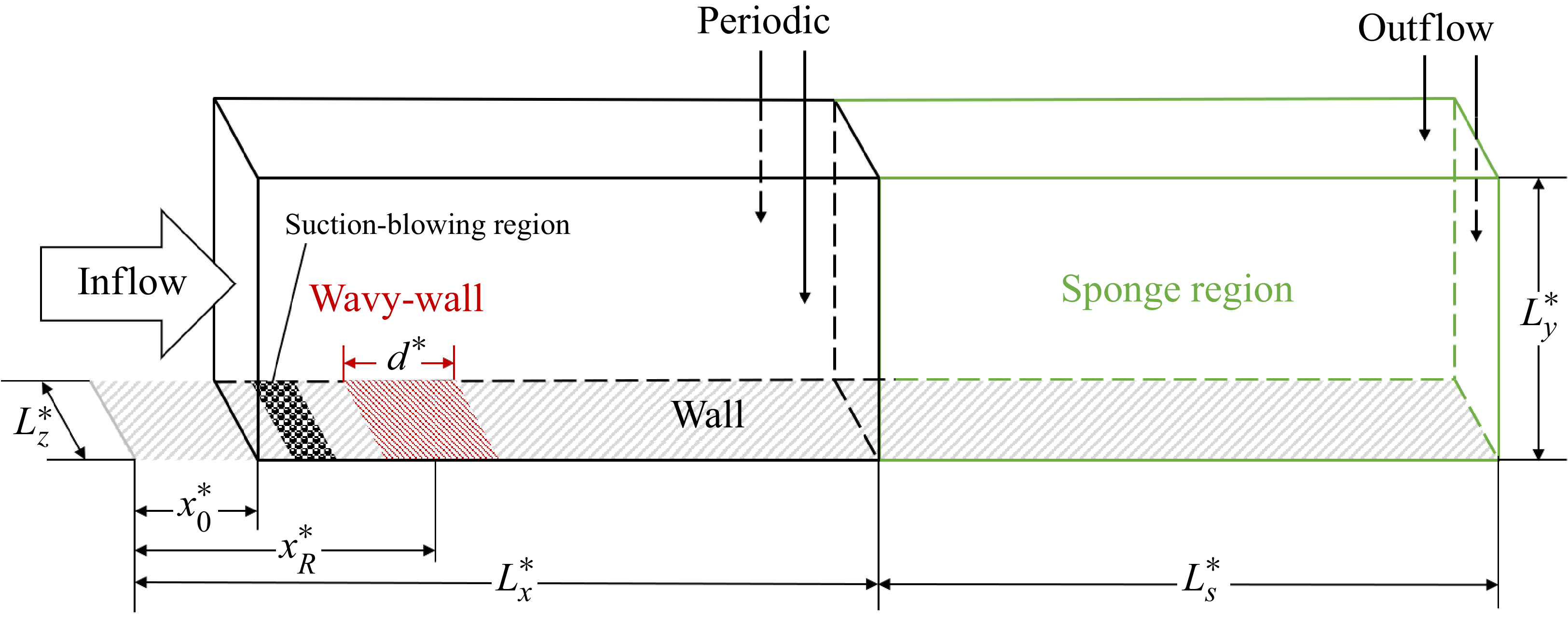
The boundary layer transition process induced by 3-D wavy wall roughness on a flat plate is studied by DNS in this paper. A sketch of the physical model and computational domain is shown in figure 1, and the boundary conditions are labelled. The self-similar solution for compressible boundary layers is introduced at the inlet of the computational domain, and its governing equations and calculation method can be found in Cebeci & Smith (Reference Cebeci and Smith1974) and Yang, Zhao & Gao (Reference Yang, Zhao and Gao2024). The outflow condition is selected at the top and right boundaries of the domain. The periodic condition is adopted on the spanwise boundary. No-slip and isothermal conditions are adopted at the wall. The scales of the computational domain are given in table 1, where the superscript * represents the dimensional value. The streamwise parameters represent the distances from the leading edge of the plate,
 $x_R^*$
is the distance from the leading edge to the centre point of the roughness region, and
 $L_s^*$
is the length of the sponge region. The simulations are performed under hypersonic conditions. The freestream parameters are chosen according to the wind-tunnel experiment by Maslov et al. (Reference Maslov, Shiplyuk, Sidorenko and Arnal2001), listed in table 2, where the subscript
 $\infty$
represents the freestream value. The wall temperature
 $T_w^*$
is set to the adiabatic temperature.
Scales of the computational domain (in units of mm).

Freestream parameters and wall temperatures for the simulation.

Sketch of the physical model and computational domain.

In this paper, two types of 3-D wavy wall roughnesses with different distribution topologies are introduced: the staggered distribution (type-S) and the aligned distribution (type-A). The heights, shapes and densities of the roughness elements are the same, while only the distribution topologies are different. The height of the rough wall can be described by
 \begin{eqnarray} y_w^*(x^*, z^*) = \left \{ \begin{array}{ll} k^*f_xg_z/4, & |x^*-x_R^*|\lt d^*/2, \\ 0, & |x^*-x_R^*|\geqslant d^*/2, \end{array} \right . \end{eqnarray}
where
 \begin{eqnarray} \begin{array}{ll} f_x=1+ \cos [2\pi (x^*-x_R^*)/\lambda _x^*],\\[3pt] g_z=1- \cos (2\pi z^*/\lambda _z^*+\theta \pi ). \end{array} \end{eqnarray}
Here,
 $\theta = \theta (x^*)$
in
 $g_z$
is used to distinguish the distribution topologies between type-S and type-A cases:
 \begin{equation} \theta (x^*) = \left \{ \begin{array}{ll} \lfloor [x^*-(x_R^*-d^*/2)]/\lambda _x^*\rfloor , & \text{type-S}, \\ 0, & \text{type-A}, \end{array} \right . \end{equation}
where
 $\lfloor {\cdot }\rfloor$
stands for rounding down, and its value represents the row number of roughness elements,
 $k^*$
represents the maximum height of the roughness, and
 $\lambda _x^*$
and
 $\lambda _z^*$
are the wavelengths of the roughness along the streamwise and spanwise directions, respectively. In this paper,
 $k^*$
is taken as 1 mm, which is 64.2
 $\,\%$
of the local undisturbed boundary layer thickness at the first roughness row. (The boundary layer edge is defined at the position where the streamwise velocity reaches 99
 $\,\%$
of the freestream velocity.) The roughness height Reynolds number of the first roughness row is
 ${\textit{Re}}_{kk}=477$
, which is sufficient to trigger the transition in hypersonic boundary layers. The wavelength of the roughness is
 $\lambda _x^*=\lambda _z^*=10$
mm.
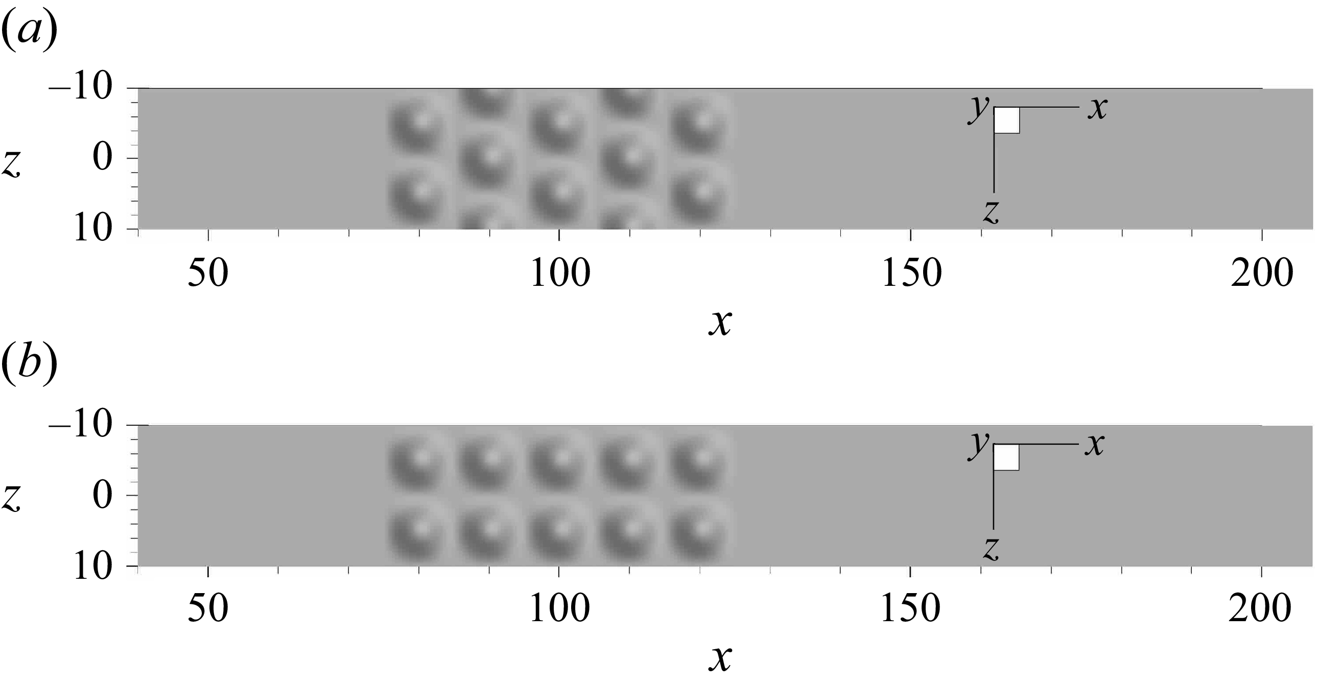
Using (2.1), the distributed roughness morphologies are generated, the top views of which are shown in figure 2, where
 $x$
and
 $z$
are non-dimensionalised with
 $k^*=1$
mm. Structured meshes are adopted for simulations in this paper. Equal-spaced meshes are used in both the streamwise and spanwise directions, with spacing
 $\Delta x^*=\Delta z^*=2\times 10^{-4}$
m, and each single roughness element contains 50 mesh points along both the streamwise and spanwise directions. Figure 3 illustrates the distribution of surface mesh points near the roughness region. The height of the first grid of the wall
 $\Delta y_w^*$
is
 $10^{-5}$
m. The total number of the mesh points (without the sponge region) is
 $n_x\times n_y\times n_z=2801\times 207\times 101=58\, 560\, 507$
. The dimensionless mesh spacings in the turbulent region are
 $\Delta x^+=\Delta z^+ = 4.36$
,
 $\Delta y_w^+=0.22$
.
Top views of (a) type-S and (b) type-A wavy wall roughness morphologies.

Distributions of surface mesh points near the (a) type-S and (b) type-A wavy wall roughness regions.

The equivalent sand grain
 $k_s$
is commonly adopted to describe the distributed roughness morphologies in turbulent flows. For transitional flows, Boyle & Stripf (Reference Boyle and Stripf2009) proposed an empirical correlation for
 $k_s$
to model the roughness effects based on their experimental results:
 \begin{equation} k_s\approx \max [4.3R_{\textit{rms}}(1+S_k),6.2R_a,4.3R_{\textit{rms}}], \end{equation}
where
 \begin{equation} R_a=\frac {\displaystyle \sum _{i = 1}^{n}\left \lvert y_i^*-\overline {y}^*\right \rvert }{n},\quad R_{\textit{rms}}=\sqrt {\frac {\displaystyle \sum _{i = 1}^{n}(y_i^*-\overline {y}^*)^2 }{n-1}},\quad S_k=\frac {\displaystyle \sum _{i = 1}^{n}(y_i^*-\overline {y}^*)^3 }{nR_{\textit{rms}}^3}. \end{equation}
Here,
 $y^*$
is the wall height,
 $\overline {y}^*$
represents the average height, and
 $n$
is the total number of the wall mesh points in the roughness region. The elements of type-S and type-A roughness have the same height, shape and distribution density. As a result, they have the same
 $k_s = 0.0033$
m according to the estimation formula (2.4), and the effects of the distribution topologies on the transition cannot be captured by this model.
2.2. Governing equations and numerical methods
For the transition process induced by 3-D wavy wall roughness in the hypersonic boundary layer, the 3-D compressible Navier–Stokes equations are adopted for the simulations. In the Cartesian coordinate system, the dimensionless Navier–Stokes equations are
 \begin{align} \frac {\partial \rho }{\partial t}+\frac {\partial (\rho u_j)}{\partial x_j} &= 0, \end{align}
 \begin{align} \frac {\partial (\rho u_i)}{\partial t}+\frac {\partial (\rho u_i u_j+p\delta _{ij})}{\partial x_j} &= \frac {\partial \tau _{ij}}{\partial x_j},\quad i=1,2,3, \end{align}
 \begin{align} \frac {\partial (\rho E)}{\partial t}+\frac {\partial (\rho Eu_j+pu_j)}{\partial x_j} &=\frac {\partial }{\partial x_j}(\tau _{ij}u_i-q_j). \end{align}
The dimensionless state equation for gas is
 \begin{equation} p=\frac {\rho T}{\gamma Ma_\infty ^2}, \end{equation}
where
 $\rho$
,
 $u_j$
,
 $T$
and
 $p$
are the density, velocity, temperature and pressure of the flow. The freestream quantities
 $\rho _\infty ^*$
,
 $u_\infty ^*$
,
 $T_\infty ^*$
and
 $\rho _\infty ^*u_\infty ^{*2}$
, are used for their non-dimensionalisations, respectively. Also,
 $\delta _{ij}$
represents the Kronecker symbol:
 $\delta _{ij}=1$
when
 $i=j$
, otherwise
 $\delta _{ij}=0$
. The spatial coordinate
 $x_j$
and time
 $t$
are non-dimensionalised by
 $L^*$
and
 $L^*/u_\infty ^*$
, respectively. In the following, the roughness height (
 $k^*=1$
mm) is taken as the reference length
 $L^*$
,
 $\tau _{ij}$
represents the shear tensor,
 \begin{equation} \tau _{ij}=\frac {\mu }{Re}\left(\frac {\partial u_i}{\partial x_j}+\frac {\partial u_j}{\partial x_i}-\frac {2}{3}\frac {\partial u_k}{\partial x_k}\delta _{ij}\right), \end{equation}
 $\mu$
is the viscosity coefficient calculated by Sutherland’s law,
 \begin{equation} \mu =T^{3/2}\frac {1+C}{T+C}, \end{equation}
with
 $C=C^*/T_\infty ^*$
, where
 $C^*$
is the Sutherland constant (
 $C^*=110.4$
K for air),
 $E=C_vT+u_k^2/2$
is the total energy, and
 $C_v$
is the specific heat at constant volume. Also,
 $q_j$
represents the heat flux term,
 \begin{equation} q_j=-\frac {\mu }{(\gamma -1)\,Ma_\infty ^2\,\textit{PrRe}}\frac {\partial T}{\partial x_j}, \end{equation}
and
 $Re$
represents the Reynolds number
 $Re=\rho _\infty ^* u_\infty ^*L^*/\mu _\infty ^*$
, where
 $Ma_\infty$
is the freestream Mach number. The specific heat ratio
 $\gamma$
is set to 1.4. The Prandtl number
 $Pr$
is taken as 0.72.
For high-accuracy numerical simulations of hypersonic boundary layer transition, a hybrid scheme is adopted for the discretisation of the inviscid fluxes. In the smooth region, the inviscid fluxes are discretised by the seventh-order upwind scheme (Dang et al. Reference Dang, Liu, Guo, Duan and Li2022). While in the discontinuity region, the seventh-order weighted essential non-oscillatory (WENO) scheme (Jiang & Shu Reference Jiang and Shu1996) is adopted. The discontinuity is detected by a Ducros sensor (Ducros et al. Reference Ducros, Ferrand, Nicoud, Weber, Darracq, Gacherieu and Poinsot1999). The value of the sensor
 $\varTheta$
is calculated by
 \begin{equation} \varTheta =\frac {(\boldsymbol{\nabla }\boldsymbol{\cdot }u)^2}{(\boldsymbol{\nabla }\boldsymbol{\cdot }u)^2+(\boldsymbol{\nabla }\times u)^2+\varepsilon }, \end{equation}
where
 $\varepsilon$
is adopted to avoid the denominator being zero:
 $\varepsilon =(u_\infty /\delta _0)^2$
(Pirozzoli Reference Pirozzoli2011), where
 $\delta _0$
denotes the incoming boundary layer thickness. Here,
 $\varTheta$
is a value between 0 and 1. When
 $\varTheta$
is bigger than a critical value
 $\varTheta _c$
, the flow is regarded as a discontinuity. In this paper,
 $\varTheta _c$
is set to 0.2. In the present simulations, the discontinuities mainly appear during the establishment of the flow field. Since the simulation starts from a uniform flow field set by the inflow profile, discontinuities arise from the interaction between the roughness and the initial flow field. While in the fully-developed flow field, the seventh-order upwind scheme is adopted for nearly all the cells, except for only a few cells in the turbulent region. The viscous fluxes are discretised by the second-order central scheme. The three-step third-order Runge–Kutta method (Shu & Osher Reference Shu and Osher1988) is adopted for the time marching. An in-house code based on the finite-difference method is used for the simulations, and its ability to simulate the hypersonic boundary layers has been fully verified (Mo et al. Reference Mo, Li, Zhang and Gao2023; Mo & Gao Reference Mo and Gao2024; Wang & Gao Reference Wang and Gao2024).
3. Results and discussion
3.1. Transition processes induced by type-S and type-A roughnesses
Unsteady DNS are carried out for the transition process induced by the wavy wall roughnesses designed in § 2.1. The perturbation is introduced into the boundary layer by unsteady random wall suction–blowing upstream of the roughness. The wall-normal velocity at the suction–blowing region is
 \begin{equation} v_w (x,z,t)=2\,\varPi (0.5-\phi ), \end{equation}
where
 $\phi =\phi (x,z,t)$
is a random number uniformly distributed between 0 and 1. The amplitude of the perturbation
 $\varPi$
is set to 1 %, which is sufficient to trigger transition downstream, yet not so strong as to cause the flow distortion. The suction–blowing is in the range
 $45\lt x\lt 55$
. The wall pressure in the suction–blowing region at
 $x=50$
across the whole spanwise domain is monitored, and figure 4 presents its spectral energy in the frequency–wavenumber space obtained by 2-D Fourier transform. It can be seen that the wall suction–blowing excites disturbances across a broad range of the frequencies and spanwise wavenumbers with nearly uniform intensity.
Spectral energy of suction–blowing disturbance in frequency–wavenumber space.

A constant time step
 $5\times 10^{-9}$
s is employed. The simulations cover approximately six flow-through times. A simulation for a smooth surface is also performed for comparison. Figure 5 shows the transition processes by the iso-surfaces of the
 $Q$
criterion (
 $Q=0.02$
) coloured by
 $u$
, where
 $Q$
is defined by
 \begin{equation} Q=-\frac {1}{2}\left[\left(\frac {\partial u}{\partial x}\right)^2+\left(\frac {\partial v}{\partial y}\right)^2+\left(\frac {\partial w}{\partial z}\right)^2\right]-\left(\frac {\partial u}{\partial y} \frac {\partial v}{\partial x}+\frac {\partial u}{\partial z} \frac {\partial w}{\partial x}+\frac {\partial v}{\partial z} \frac {\partial w}{\partial y}\right). \end{equation}
Iso-surfaces of the
 $Q$
criterion (
 $Q=0.02$
) of the instantaneous flowfield for (a) type-S, (b) type-A, and (c) smooth cases.

It can be seen from figure 5(a) that downstream of the type-S roughness, the flow begins to destabilise at approximately
 $x=350$
, and broken structures with multiple scales are observed downstream. However, for the type-A roughness as shown in figure 5(b), the flow does not destabilise until approximately
 $x=500$
, and some coherent structures, such as horseshoe vortices, can still be found near the outlet of the computational domain at
 $x=600$
, which indicates that the flow has not completely broken down in the computational domain. It can be seen that the transition-inducing ability of type-S roughness is significantly stronger than that of type-A roughness. For the smooth case, no vortex structures are obtained under the same value of
 $Q$
. Figure 6 shows the time- and spanwise-average
 $u$
profiles at the end of the computational domain. The compressible self-similar solution for the laminar boundary layer is also included. It can be seen that the profile of the smooth case agrees well with the self-similar result, indicating that the flow remains laminar over the whole domain, and the transition is promoted in both roughness cases.
Time- and spanwise-average
 $u$
profiles at
 $x=600$
for all three cases.

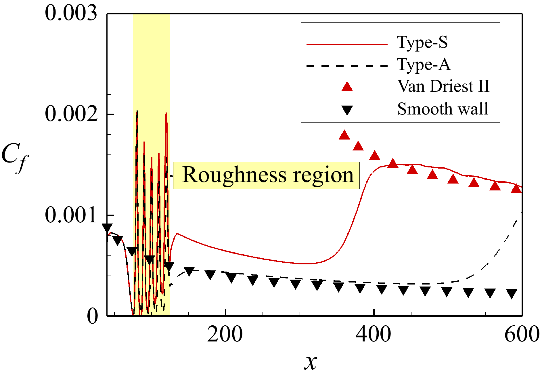
Figure 7 gives the development of time- and spanwise-average skin friction coefficient
 $C_f=\tau _w^*/(\rho _\infty ^* u_\infty ^{*2} /2)$
along the streamwise direction. It can also be observed from
 $C_f$
that the transition induced by type-S roughness is significantly earlier than type-A. The
 $C_f$
curve of type-S roughness agrees well with the theory value of Van Driest II (Franko & Lele Reference Franko and Lele2013) in the region
 $x\gt 400$
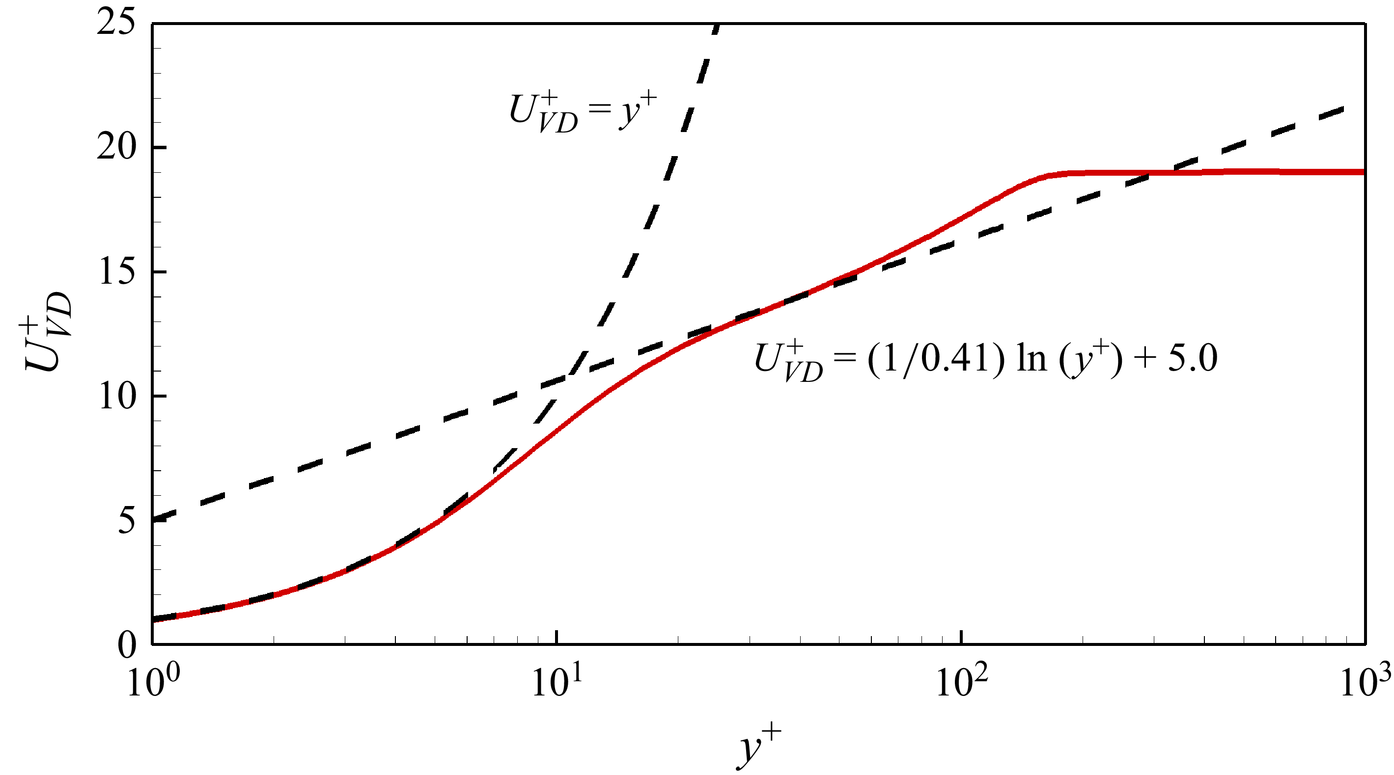
. In addition, figure 8 shows the Van Driest transformed time- and spanwise-average
 $u$
profile for the type-S case at
 $x=500$
, and it agrees well with the viscous sublayer law
 $U_{VD}^+=y^+$
and the log law
 $U_{VD}^+=(1/0.41)\ln (y^+)+5.0$
. It is indicated that downstream of type-S roughness, the boundary layer has completely turned to turbulence within the computational domain. However,
 $C_f$
of the type-A case does not even reach the Van Driest II value within the computational domain, indicating that the transition process is not completed. Defining the transition-onset position
 $x_t$
as the intersection point of the extension lines from the laminar and transitional
 $C_f$
curves, as shown in Appendix A,
 $x_t$
values for type-S and type-A cases are 342 and 522, respectively. The corresponding transition-onset Reynolds numbers
 ${\textit{Re}}_{xt}$
are
 $4.5\times 10^6$
and
 $6.9\times 10^6$
, respectively. The transition induced by type-S roughness is 34.5 % earlier than that of type-A roughness.
Development of time- and spanwise-average skin friction coefficient
 $C_f$
along the streamwise direction.

The Van Driest transformed
 $u$
profile at
 $x=500$
for the type-S case.

In conclusion, the distribution topology of roughness has significant effects on the transition, so
 ${\textit{Re}}_{kk}$
and the estimation model for
 $k_s$
(Boyle & Stripf Reference Boyle and Stripf2009) are both incomplete. Furthermore, the type-S roughness can induce transition significantly earlier than type-A roughness. To reveal the mechanisms of this phenomenon, the flow structures and the stability characteristics of the two roughnesses will be studied in detail in the following subsections.
3.2. Differences in flow structures between type-S and type-A roughnesses
In this subsection, based on the time-average results of DNS, the differences in the flow structures between the type-S and type-A cases are investigated.
Figure 9 plots the flow field near the roughness, including the streamlines near the wall, pressure on
 $x{-}y$
planes, and the distributions of streamwise vorticity
 $\omega _x$
and velocity
 $u$
on
 $y$
–
 $z$
planes downstream of the roughness, where
 $\omega _x=\partial w/\partial y-\partial v/\partial z$
. It can be seen that the streamlines are curved near the roughness region, and a series of compression and expansion waves is induced. Figure 10 gives the distributions of wall pressure
 $p_w$
and wall pressure gradient
 $\partial p_w/\partial x$
around the roughness:
 $p_w$
experiences an oscillation in the roughness region, and recovers to the smooth-case value a short distance downstream of the roughness. The pressure gradient is governed by the surface curvature, with the peaks of the roughness elements experiencing a favourable pressure gradient, and the valleys, conversely, an adverse gradient.
Flow structures near the (a) type-S and (b) type-A roughnesses.

Distributions of (a,b) wall pressure
 $p_w$
and (c,d) wall pressure gradient
 $\partial p_w/\partial x$
along the streamwise direction for type-S and type-A cases. The blue and yellow blocks represent the locations of the windward side and leeward side of roughness elements.

As shown in figure 9, counter-rotating pairs of streamwise vortices are generated downstream. Type-S roughness generates significantly stronger vortices than type-A roughness, and in turn introduces more significant flow distortion downstream. Figure 11 shows the development of
 $\omega _{x,max }$
(the local maximum of
 $\omega _x$
) along the streamwise direction, and the red dash-dotted line gives the ratio of
 $\omega _{x,max }$
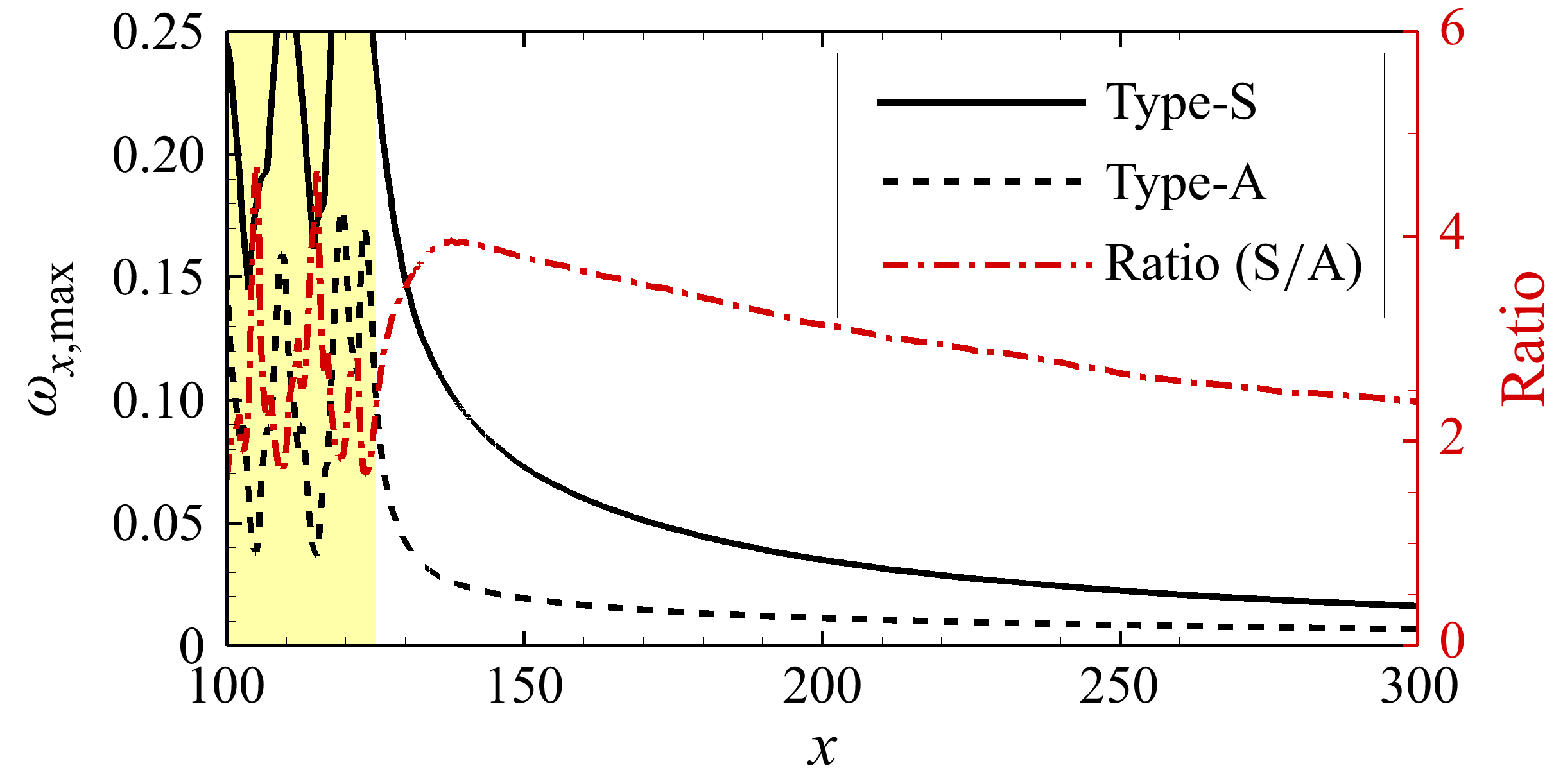
of the type-S case to that of the type-A case. As shown in the figure, the vortex intensity downstream of type-S roughness is approximately 2–4 times that of type-A roughness. The counter-rotating pairs of vortices can induce the flow distortion. Figure 12 shows the distribution of
 $\omega _x$
and
 $u$
(black contour lines) in the
 $y$
–
 $z$
plane at
 $x=150$
and 250 downstream of the roughness, where the relationship of vortices and flow distortion can be seen more clearly. As the counter-rotating vortices develop downstream, they can pull high-velocity fluids towards the wall and lift low-velocity fluids upwards, as indicated by the green arrows in the figure. This mechanism leads to flow distortion, characterised by high- and low-velocity streaks. The flow distortion becomes more significant as it moves downstream, which is significantly stronger in the type-S case than the type-A case.
Development of
 $\omega _{x,max }$
along the streamwise direction. The red dash-dotted line represents the ratio of the type-S case to the type-A case.

Distribution of
 $\omega _x$
in the
 $y$
–
 $z$
plane downstream of the roughness. The black lines represent the contour lines of
 $u$
.

In order to explain the stronger vortices in the type-S case, the generation mechanism of the streamwise vortices is analysed next. Three representative
 $y$
–
 $z$
slices are extracted as shown in figure 13, located on the windward side of the first row of the roughness (
 $x=78$
, slice I), the leeward side of the first row (
 $x=82$
, slice II), and the windward side of the second row (
 $x=88$
, slice III), respectively. Since the flow is periodic along the spanwise direction, only the region
 $0\lt z\lt 10$
of the slices is shown. The distributions of
 $w$
in the slices are given at the top of figure 13, and the distributions of
 $\omega _x$
as well as its components (
 $\partial w/\partial y$
,
 $\partial v/\partial z$
) are given at the bottom.
Development of the streamwise vortices in (a) type-S and (b) type-A cases. Slices I, II and III are extracted at
 $x=78$
, 82 and 88, respectively. The distributions of
 $w$
,
 $\omega _x$
and
 $(\partial w/\partial y,\partial v/\partial z)$
in the slices are given from the top to the bottom of the panels.

At slices I and II, the two types of roughness have similar mechanisms for inducing streamwise vortices. As can be seen from the
 $w$
distributions in figure 13, when the flow arrives at the windward side of the first row of the roughness element, significant spanwise velocity is induced, which makes the flow horizontally bypass the roughness element. Meanwhile, vortices are induced near the wall, and the vortices on the left- and right-hand sides of the roughness element have the same strength and opposite rotating direction. Based on the comparison of the components
 $\partial w/\partial y$
and
 $\partial v/\partial z$
at the bottom of the figure, it can be obtained that the formation of the vortices is dominated by the component
 $\partial w/\partial y$
, i.e. the vortices are mainly generated by the flow travelling horizontally around the roughness element. In contrast, the contribution of the lift-up mechanism (
 $\partial v/\partial z$
) by the roughness element can be ignored. As the flow travels downstream to the leeward side of the roughness element, as shown at slice II in figure 13, the distribution of
 $w$
indicates that the flow is clustered towards the centreline. Meanwhile, streamwise vortices with the opposite direction to the vortices on slice I are induced. By comparing the components
 $\partial w/\partial y$
and
 $\partial v/\partial z$
, it can be concluded that the vortices at slice II are still governed by
 $\partial w/\partial y$
, i.e. by the flow clustering from the sides of the roughness element towards the centreline.
When the flow travels at slice III, as shown in figure 13, the vortex-inducing mechanisms of the type-S and type-A roughnesses appear to be different. Due to the staggered arrangement of type-S roughness elements, the windward side of the second row can induce
 $w$
in the same direction as the leeward side of the first row, which results in constructive vortex superposition. As a result, the vortices induced at the leeward side of the first row are enhanced on the windward side of the second row, which is named the ‘staggered-enhancing’ mechanism in this paper. Due to this mechanism, the leeward side vortices of each row of the roughness elements will be enhanced by their downstream elements, so the vortices get stronger as they travel downstream in the type-S case. However, for the type-A roughness, the windward side of its second row element induces vortices in the opposite direction to the vortices at the leeward side of the first row, which makes the development of the vortices destructive. Similarly, as the flow travels downstream, the above processes will be repeated until the flow passes the roughness region.
To clarify the relative magnitude between
 $\partial w/\partial y$
and
 $\partial v/\partial z$
, figure 14 shows the local maxima of
 $|\omega _x|$
,
 $|\partial w/\partial y|$
and
 $|\partial v/\partial z|$
along the
 $z$
-direction on the three slices above. It can be seen clearly that the streamwise vortices are dominated by
 $\partial w/\partial y$
at all the slices. In addition, the staggered-enhancing’ effects can be observed by comparing figures 14(e) and 14(f).
Local maxima of
 $|\omega _x|$
,
 $|\partial w/\partial y|$
and
 $|\partial v/\partial z|$
along the
 $z$
-direction on slices I, II and III, for (a,c,e) type-S and (b,d,f) type-A cases, respectively. Results on slices I, II and III are displayed from top to bottom.

To understand the generation of streamwise vortices downstream of the roughness, some slices near the end of the roughness are also extracted, as shown in figure 15. Figure 16 shows the distributions of
 $\omega _x$
on the slices, and the evolutions of the streamwise vortices are traced. In the type-S case, the downstream counter-rotating streamwise vortex pairs are generated from the leeward side of the third and fourth roughness rows, as shown on slices IV and VI, respectively. Then they undergo the staggered-enhancing processes at the windward sides of their subsequent roughness rows, as shown on slices V and VII, which finally results in their high strength. In the type-A case, the downstream vortex pairs are generated directly from the windward and leeward sides of the last roughness row, as shown on slices IX and X. They do not undergo an enhancing process, which results in their weaker strength.
Locations of the slices extracted near the end of the roughness regions of (a) type-S and (b) type-A cases.

Distributions of
 $\omega _x$
on slices around the ends of the roughness regions of (a) type-S and (b) type-A cases.

To provide a global perspective of the evolution of vortices, based on the iso-surfaces of
 $\omega _x=\pm 0.2$
, the differences between the developments of the streamwise vortices of type-S and type-A roughnesses through the whole roughness region are illustrated in figure 17. The iso-surfaces of the components
 $\partial w/\partial y$
and
 $\partial v/\partial z$
are also given on the right-hand side of the figure. It can be seen that the contribution of
 $\partial v/\partial z$
to the streamwise vortices can be negligible compared to
 $\partial w/\partial y$
, which indicates that streamwise vortices are generated by the flow horizontally bypassing the roughness over the whole roughness region for both cases. In addition, due to the staggered-enhancing mechanism, the development of the vortices is more continuous along the streamwise direction in the type-S case. On the contrary, the contribution of each row of type-A roughness to the development of the vortices is relatively isolated. As a result, type-S roughness can induce significantly stronger streamwise vortices compared to type-A roughness.
Development of streamwise vortices near the (a) type-S and (b) type-A roughness regions. The left-hand side of the figure shows the iso-surfaces of
 $\omega _x = \pm 0.2$
, while the right-hand side shows the iso-surfaces of
 $\partial w/\partial y=\pm 0.2$
and
 $\partial v/\partial z=\pm 0.2$
.

Since type-S roughness induces stronger streamwise vortices, it can induce more significant flow distortion, which in turn introduces stronger shear action. Define the local shear strength
 $u_s$
to describe the shear action quantitatively:
 \begin{equation} u_s=\sqrt {\left(\frac {\partial u}{\partial y}\right)^2+\left(\frac {\partial u}{\partial z}\right)^2}. \end{equation}
Figure 18 gives the distribution of
 $u_s$
in the
 $y$
–
 $z$
plane at
 $x=200$
for the two cases, and the black lines represent the contour lines of
 $u$
. As shown in the figure,
 $u_s$
downstream of the type-S roughness is significantly higher than that for the type-A roughness, which is also a key factor governing the transition process, as will be demonstrated in the following analysis. The shear action mainly occurs in the near-wall region and near the edge of the boundary layer, where the shear structure near the boundary layer edge is referred to as the shear layer in this paper. In addition, in the near-wall region, the high shear strength of the type-S roughness also leads to higher wall friction compared to the type-A roughness, even in the laminar region. For example, as shown in figure 7, the spanwise-average laminar friction coefficient
 $C_f$
of the type-S case is approximately 1.5 times that of the type-A case at
 $x=200$
.
Distribution of the shear strength
 $u_s$
in the
 $y$
–
 $z$
plane at
 $x=200$
of (a) type-S and (b) type-A cases. The black lines represent the contour lines of
 $u$
.

3.3. Propagation process of fluctuation downstream of roughness
In this subsection, the spatial developments of the fluctuation downstream of type-S and type-A wavy wall roughnesses are studied, including the linear and nonlinear stages.
According to the statistical results of DNS, the development of
 $u_{\textit{rms}}^\prime$
(the root mean square of
 $u$
fluctuation) along the streamwise direction is given in figure 19. The instantaneous friction coefficients
 $C_f$
are also given at the wall to illustrate the transition process. Here,
 $u_{\textit{rms}}^\prime$
is normalised with the local maximum value
 $u_{\textit{rms,max}}^\prime$
, and the development of
 $u_{\textit{rms,max}}^\prime$
along the streamwise direction is given in figure 20. The velocity fluctuation is amplified along the streamwise direction, and the intensity of the type-S case is always higher than that of the type-A case. In the roughness region,
 $u_{\textit{rms,max}}^\prime$
experiences an oscillation along the streamwise direction due to the variations in pressure gradient. The disturbance decays in the favourable pressure gradient regions at the peaks of each roughness element, and amplifies in the adverse pressure gradient regions at the valleys. Downstream of the type-S roughness,
 $u_{\textit{rms,max}}^\prime$
is approximately constant as
 $x\gt 400$
, where the flow has turned into turbulence. As shown in figure 19, before the transition occurs,
 $u_{\textit{rms}}^\prime$
for both type-S and type-A cases is concentrated at the shear layer. This stage corresponds to the linear development of the fluctuation, indicating that the increase in linear fluctuation is dominated by shear layer instability. For type-S roughness, as the shear layer fluctuation grows to a critical strength, the nonlinear breakdown is triggered, and the fluctuation region rapidly spreads to the near-wall region. Finally, the fluctuation is concentrated at the wall, corresponding to the characteristics of the turbulent flow. However, for type-A roughness, the fluctuation region does not start to spread until
 $x$
reaches 500, corresponding to the beginning of the nonlinear stage, and its transition process is not completed within the computational domain.
Development of
 $u_{\textit{rms}}^\prime$
downstream of (a) type-S and (b) type-A roughnesses. The instantaneous friction coefficients
 $C_f$
are given at the wall.

Development of
 $u_{\textit{rms,max}}^\prime$
along the streamwise direction.

Figure 21 plots the temporal power spectral density (PSD) of
 $u$
probed at the locations of peak
 $u_{\textit{rms}}^\prime$
at different streamwise locations for both cases. For the type-S case, as shown in figure 21(a), the PSD curves in the laminar region (
 $x=300,400$
) exhibit peaks near 50 kHz. The magnitude of the PSD increases along the streamwise direction. Finally, in the turbulent region (
 $x=400,500$
), the high-frequency PSD increases and finally exhibits the
 $-5/3$
power-law region (representing the inertial subrange of the turbulence). However, for the type-A case, as shown in figure 21(b), the PSD curves at all the locations exhibit peaks in the high-frequency region near 120 kHz. The magnitude of the PSD also increases along the streamwise direction, but it does not establish the
 $-5/3$
power-law region.
Temporal PSD of
 $u$
probed at different streamwise locations for (a) type-S and (b) type-A cases.

To indicate the unsteadiness at the wall, figure 22 shows the distributions of
 $C^\prime _{f{,rms}}$
over the whole domain for both cases. It is indicated that the disturbances at the wall are also characterised by streak structures in the laminar region. Their peak fluctuations are located directly underneath the peak fluctuations in the shear layer. The unsteadiness at the wall of the type-S case is stronger than that of the type-A case.
Distributions of
 $C^\prime _{f{,rms}}$
over the domain for (a) type-S and (b) type-A cases.

In order to seek the dominant mode of the instability, the SPOD analysis is carried out, where SPOD is a data-driven modal analysis method. Unlike the traditional proper orthogonal decomposition (POD) method, which only seeks spatially coherent modes, SPOD can capture modes that are coherent in both space and time (Taira et al. Reference Taira, Brunton, Dawson, Rowley, Colonius, McKeon, Schmidt, Gordeyev, Theofilis and Ukeiley2017, Reference Taira, Hemati, Brunton, Sun, Duraisamy, Bagheri, Dawson and Yeh2020; Towne, Schmidt & Colonius Reference Towne, Schmidt and Colonius2018). In practice, SPOD analysis requires the time sequence of the flow field
 $\unicode{x1D64C}$
as the input:
 \begin{equation} {\unicode{x1D64C}}=[\boldsymbol{q}_1,\ldots ,\boldsymbol{q}_i,\ldots ,\boldsymbol{q}_N]. \end{equation}
The vector
 $\boldsymbol{q}_i$
represents the snapshot of the flow field at moment
 $i$
, and
 $N$
is the total number of snapshots. In this paper, the time sequence results from DNS are adopted for the SPOD analysis. To obtain convergent estimates of spectral densities, it is necessary to split
 $\unicode{x1D64C}$
into multiple blocks, and average the spectral density of each block as the final result. The Welch (Reference Welch1967) method is used for splitting here, and the
 $k$
th block of the data can be written as
 \begin{equation} {\unicode{x1D64C}}_k=[\boldsymbol{q}_{s+1},\boldsymbol{q}_{s+2},\ldots ,\boldsymbol{q}_{s+N_k}], \end{equation}
where
 $N_k$
is the number of snapshots in the
 $k$
th block. The subscript
 $s$
begins at
 $(k-1)(N_k-N_o)$
, where
 $N_o$
represents the number of snapshots overlapping between the blocks. The SPOD is implemented based on the open source code by Schmidt & Colonius (Reference Schmidt and Colonius2020).
The time sequence of
 $u$
in the
 $x$
–
 $y$
plane at
 $z=0$
is extracted first, and the SPOD parameters are set with reference to Lin & Schmidt (Reference Lin and Schmidt2024) and Guo, Hao & Wen (Reference Guo, Hao and Wen2025), who both carried out SPOD analysis on transition boundary layers. The physical sampling time interval is
 $\Delta t_{\textit{snap}}^*=2.5\times 10^{-7}$
s, corresponding to sampling frequency
 $f_{\textit{snap}}^*=4$
MHz. The total sampling time is
 $1.2\times 10^{-3}$
s, corresponding to recognisable minimum frequency 1.67 kHz. The total sampling number is
 $N=4801$
. The samples are divided into multiple blocks, and the length of a single block is
 $N_k=512$
, with
 $N_o/N_k=75\,\%$
overlapping.
Figure 23 shows the development of the local maximum of
 $u$
fluctuation strength corresponding to the leading SPOD modes at different frequencies. For type-S roughness, as shown in figure 23(a), the development of the fluctuation downstream of the roughness is divided into three stages, i.e. linear instability, nonlinear breakdown, and turbulence. In the linear stage at
 $x\lt 350$
, the instability is dominated by low-frequency modes with frequencies below 60 kHz. As the low-frequency fluctuations arrive at
 $x\approx 350$
(as shown by the black arrow in the figure), the amplitudes of the low-frequency fluctuations saturate, and the high-frequency fluctuations are rapidly excited, corresponding to the high-frequency secondary instability process. The flow then comes to the nonlinear breakdown stage. Selecting two representative frequencies, 47 kHz and 500 kHz, the developments of their corresponding
 $u$
fluctuations of the leading SPOD
 $x$
–
 $y$
modes are plotted in figure 24. As shown in figure 24(a), the low-frequency fluctuation exists over a wide range in the streamwise direction. It has only a single peak along
 $y$
near the shear layer at
 $x\lt 350$
, corresponding to the low-frequency shear layer instability. For the 500 kHz high-frequency fluctuation, as shown in figure 24(b), it disappears at the upstream region and emerges from
 $x\approx 350$
, representing the onset of nonlinear breakdown. Moreover, the high-frequency fluctuation appears from the shear layer, indicating that the nonlinear breakdown process begins from the shear layer and then spreads to the near-wall region. Figure 25 shows the distribution of the instantaneous shear strength
 $u_s$
in the
 $x$
–
 $y$
plane at
 $z=0$
downstream of type-S roughness, which visualises the nonlinear breakdown process of the shear layer.
Development of the local maximum of
 $u$
fluctuation intensity of the leading SPOD
 $x$
–
 $y$
modes at
 $z=0$
for (a) type-S and (b) type-A cases.

Development of
 $u$
fluctuations of the leading SPOD
 $x$
–
 $y$
modes at (a) 47 kHz and (b) 500 kHz at
 $z=0$
of the type-S case.

Instantaneous
 $u_s$
in the
 $x$
–
 $y$
plane at
 $z=0$
downstream of type-S roughness.

For the type-A roughness case, the dominant modes of its linear instability shift to high-frequency modes above 100 kHz, as shown in figure 23(b). Figure 26 plots the
 $u$
fluctuation of the leading SPOD
 $x$
–
 $y$
mode at 133 kHz downstream of type-A roughness. It can be seen that, unlike the shear layer instability of the type-S case in figure 24(a),
 $u^\prime$
in figure 26 exhibits several peaks along
 $y$
at different regions, including the near-wall region. It is indicated that there is an essential difference in the linear instability mechanism between the type-S and type-A roughnesses. In addition, the growth rate of the fluctuation downstream of type-A roughness is significantly lower than that of type-S roughness, which leads to the fact that the fluctuation downstream of type-A roughness has to undergo a longer growth path before it is sufficient to trigger nonlinear breakdown. Therefore, the transition induced by type-A roughness is significantly later than that of type-S roughness. In summary, understanding the linear instability mechanisms of the two types of roughness is key to revealing the differences in their transition mechanisms. This will be discussed in the following subsection.
Development of
 $u$
fluctuation of the leading SPOD
 $x$
–
 $y$
mode at 133 kHz at
 $z=0$
of the type-A case.

3.4. The SPOD analysis of linear dominant modes downstream of roughness
In this subsection, the SPOD method is employed to investigate the differences in linear instability mechanisms between the two types of wavy wall roughness. The time sequences of the flow field in the
 $y$
–
 $z$
plane at
 $x=200$
and 300 in the linear instability stage are extracted as the samples. The parameters of the SPOD are the same as in § 3.3. The sampling frequency is 4 MHz, and the total sampling time is
 $1.2\times 10^{-3}$
s. The total sampling number is 4801, and
 $N_k=512$
, with
 $N_o/N_k=75\,\%$
overlapping.
For type-S roughness, figure 27 shows the modal energy of the first 20 modes obtained from
 $u$
- and
 $p$
-based SPOD at
 $x=200$
and 300. As shown in figures 27(a) and 27(b), the energy of the leading
 $u$
-based SPOD mode shows significant peaks in the low-frequency region at
 $f^*=39$
and 47 kHz, respectively. No additional dominant mode is detected by the
 $p$
-based SPOD. It is indicated that the linear instability downstream of type-S roughness is dominated by low-frequency fluctuations, which is also in agreement with the conclusion in § 3.3. Furthermore, figure 28 shows the
 $n$
th modal energy at the peak frequencies 39 kHz (
 $x=200$
) and 47 kHz (
 $x=300$
). The figure indicates that the leading mode is absolutely dominant. The
 $u$
fluctuations of the leading SPOD modes are also plotted in figure 28, which indicates that the fluctuations are symmetrically distributed, and the fluctuation regions exhibit close spatial correspondence with the shear layers as shown in figure 18. In summary, downstream of the type-S roughness, the linear instability is dominated by the low-frequency shear layer instability, and the dominant mode is symmetric.
The
 $n$
th mode energy obtained from (a,b)
 $u$
-based and (c,d)
 $p$
-based SPOD for the type-S case, for (a,c)
 $x=200$
and (b,d)
 $x=300$
, respectively. The red dashed lines represent the upper and lower bounds of the 99 % confidence level for the leading modes.

The energy of the
 $n$
th
 $u$
-based SPOD
 $y$
–
 $z$
modes at the peak frequencies (a) 39 kHz,
 $x=200$
, and (b) 47 kHz,
 $x=300$
, downstream of the type-S roughness. The
 $u$
fluctuation of the leading mode is also plotted in the figure.

For type-A roughness, figure 29 presents the modal energy of the first 20 modes obtained from
 $u$
- and
 $p$
-based SPOD at
 $x=200$
and 300, respectively. As shown in figures 29(a) and 29(b), the SPOD energy of the type-A case is reduced by approximately two orders of magnitude compared to the type-S case. In addition, both the energy curves of the leading SPOD modes have two peaks, located in the low-frequency (23 kHz) and high-frequency (above 100 kHz) regions, respectively. The modal energies corresponding to the two peaks are comparable, indicating that the linear instability downstream of type-A roughness is co-dominated by these two modes. This appears inconsistent with the analysis in § 3.3, since no high-energy modes are observed in the low-frequency region, as shown in figure 23(b). Regarding this phenomenon, figure 30 gives the
 $n$
th SPOD
 $y$
–
 $z$
modes at 23 kHz as well as the velocity fluctuations for the leading modes. As shown in the figure, the low-frequency fluctuations are concentrated at the shear layer – i.e. similar to the type-S case, the low-frequency instability downstream of the type-A roughness is also induced by the shear layer instability. However, unlike the symmetric modes dominated in the type-S case, the shear layer instability in the type-A case is dominated by antisymmetric modes. The fluctuation strength of antisymmetric modes is close to zero at
 $z=0$
. As a result, the low-frequency fluctuations were not captured in the
 $x$
–
 $y$
SPOD analysis at
 $z=0$
downstream of type-A roughness in § 3.3. For the dominant modes in the high-frequency region, the
 $p$
-based SPOD analysis also captures the energy peaks at 133 and 109 kHz, as shown in figures 29(c) and 29(d), and the peak energy is more significant compared with the result of
 $u$
-based SPOD, which indicates that the high-frequency modes exhibit the characteristics of the acoustic mode. The distributions of
 $p$
fluctuations of the leading SPOD
 $y$
–
 $z$
modes in figure 31 indicate that the fluctuation is mainly concentrated at
 $z=0$
and
 $\pm 10$
, and the fluctuations have two strength peaks along the wall-normal direction, which is the characteristic of Mack’s second mode (Mack Reference Mack1984). In addition, the frequency of the dominant mode also matches Mack’s second mode frequency predicted by linear stability analysis, as shown in Appendix B. The dominant frequency decreases along the
 $x$
-direction, which is also consistent with the result by linear stability analysis. It follows that the high-frequency instability downstream of the type-A roughness is induced by Mack’s second mode. In summary, the linear instability downstream of the type-A roughness is co-dominated by two modes: the antisymmetric shear layer instability mode in the low-frequency region, and Mack’s second mode in the high-frequency region. Both modes are significantly weaker than the dominant shear layer instability downstream of the type-S roughness.
The
 $n$
th mode energy obtained from (a,b)
 $u$
-based and (c,d)
 $p$
-based SPOD for the type-A case, for (a,c)
 $x=200$
and (b,d)
 $x=300$
, respectively. The red dashed lines represent the upper and lower bounds of the 99 % confidence level for the leading modes.

The energy of the
 $n$
th
 $u$
-based SPOD
 $y$
–
 $z$
modes at peak frequency 23 kHz at (a)
 $x=200$
and (b)
 $x=300$
downstream of type-A roughness. The
 $u$
fluctuation of the leading mode is also plotted in the figure.

The energy of the
 $n$
th
 $p$
-based SPOD
 $y$
–
 $z$
modes at the peak frequencies (a) 133 kHz,
 $x=200$
, and (b) 109 kHz,
 $x=300$
, downstream of type-A roughness. The
 $p$
fluctuation of the leading mode is also plotted in the figure.

To provide a 3-D perspective of the dominant modes, the 3-D flow field near
 $x=300$
is monitored, and 3-D SPOD is performed. Figure 32 plots the iso-surfaces of
 $u'$
of the leading 3-D SPOD modes at low frequencies for both cases. The dominant symmetric and antisymmetric modes are clearly observed in type-S and type-A cases, respectively. At high frequency 110 kHz, figure 33 shows the iso-surfaces of
 $u'$
and
 $p'$
of the leading SPOD mode for the type-A case. The multi-peak structures along the wall-normal direction can be clearly observed, and the disturbances are concentrated near
 $z=0$
and
 $\pm 10$
.
Iso-surfaces of the leading 3-D SPOD mode
 $u'$
at low frequencies for (a) type-S (45 kHz) and (b) type-A (25 kHz) cases.

Iso-surfaces of the leading 3-D SPOD mode (a)
 $u'$
and (b)
 $p'$
at high frequency 110 kHz for the type-A case.

4. Conclusions
In this paper, the transition processes induced by 3-D wavy wall roughnesses with two different distribution topologies (staggered type-S, and aligned type-A) under
 $Ma=5.92$
are studied using DNS, and the effects of the two distribution topologies on transition are investigated for the first time. The roughness elements in the two cases are designed to have the same height, shape and distribution density. The two types of roughness have the same
 ${\textit{Re}}_{kk}$
and the same equivalent sand grain roughness height
 $k_s$
calculated by the empirical correlation of Boyle & Stripf (Reference Boyle and Stripf2009), differing solely in distribution topology. The effect mechanisms of the distribution topology on the transition are studied from the perspectives of the flow structure and the instability characteristics of the flow field. The main conclusions are as follows.
It is found that the type-S and type-A roughnesses have significantly different effects on boundary layer transition, indicating that the current estimation formula of
 $k_s$
for characterising the roughness effect on transition is incomplete. The transition induced by type-S roughness is significantly earlier, approximately 34.5 % earlier than that of type-A roughness under the conditions in this paper.
For the flow structure, both type-S and type-A roughnesses can induce counter-rotating pairs of streamwise vortices. The vortices are mainly induced by the
 $\partial w/\partial y$
term, i.e. by the flow horizontally bypassing the roughness elements. For type-S roughness, a staggered-enhancing mechanism for the streamwise vortices between the roughness elements is found: since the direction of the vortices induced by the windward side of the roughness element is the same as the direction of vortices in the wake of its upstream roughness element, the vortices will be enhanced as they travel downstream. However, this mechanism does not exist between the elements of type-A roughness. As a result, type-S roughness can induce significantly stronger streamwise vortices, the strength of which can be nearly 2–4 times that of type-A roughness. Furthermore, stronger streamwise vortices will introduce stronger shear layer structures downstream, which is the key factor leading to the stronger transition-inducing ability of type-S roughness.
Based on the time sequence data of DNS, the SPOD analysis is adopted to reveal the linear/nonlinear instability characteristics of the two roughnesses. For type-S roughness, its downstream linear instability is dominated by the low-frequency shear layer instability near 50 kHz, which is symmetric in the spanwise direction and exhibits a high spatial growth rate. During the whole linear instability process, the fluctuations are concentrated at the shear layer. Once the linear fluctuation amplitude saturates, the nonlinear breakdown is triggered from the shear layer, and the flow ultimately undergoes transition to turbulence. Then for type-A roughness, its downstream linear instability is co-dominated by two modes: the low-frequency shear layer instability near 23 kHz, and the high-frequency Mack’s second mode above 100 kHz. The shear layer instability is antisymmetric along the spanwise direction, and both modes are significantly weaker than the dominant shear layer instability downstream of type-S roughness. As a result, the linear fluctuation downstream of type-A roughness grows more slowly, delaying the transition onset compared to the type-S case.
The cases with only two rows of roughnesss elements are also examined. The main conclusions still hold: the staggered distribution will enhance the streamwise vortices and the disturbances, and finally leads to early transition. Nevertheless, compared to the five-row configuration, the staggered-enhancing effect is significantly weaker in the two-row case, and the transition-inducing capability is also significantly reduced. The main results are provided in Appendix C.
Funding
This research is supported by the National Natural Science Foundation of China through grant nos 12372283 and U24B2007.
Declaration of interests
The authors report no conflict of interest.
Appendix A. Determination of transition onset position
The transition onset locations are determined by the intersection point of the extension lines from the laminar and transitional
 $C_f$
curves. This method has also been adopted in previous studies (Chuvakhov Reference Chuvakhov2018; Guo et al. Reference Guo, Hao and Wen2025). Figure 34 shows the
 $C_f{-}x$
curves on a log–log plot. The
 $C_f$
curves are approximately straight lines in both the laminar and transitional regions, and their extension lines intersect at a point, which is defined as the transition onset location.
Determination of the transition onset locations from the
 $C_f{-}x$
curves on a log–log plot.

Appendix B. Linear stability analysis of a boundary layer on a smooth plate
The linear stability analysis under the conditions in table 2 is performed on a smooth plate. The linear stability equations for compressible flows based on the local parallel assumption are adopted. Following the methodology of Malik (Reference Malik1990), the Chebyshev spectral collocation scheme is employed for the spatial discretisation. The numerical code for linear stability analysis has been well validated (Yang et al. Reference Yang, Zhao and Gao2024). Figure 35 gives the growth rate
 $\delta$
and
 $N$
factor of the 2-D linear instability modes over the domain, where the
 $N$
factor is the ratio of the local perturbation intensity
 $I(x)$
to its initial value
 $I_0$
:
 \begin{align} N=I/I_0=\int _{x_0}^{x}\sigma\, {\rm d} x, \end{align}
where
 $x_0$
is the neutral point. The
 $N$
factor curves of some representative frequencies are marked with different colours in figure 35(b). It can be seen that the frequency of the dominant Mack’s second mode is approximately 100–150 kHz near
 $x=200{-}300$
, and decreases along the streamwise direction.
(a) Growth rate and (b)
 $N$
factor of the 2-D linear instability modes by the local parallel assumption.

Appendix C. Results for roughnesses with only two rows
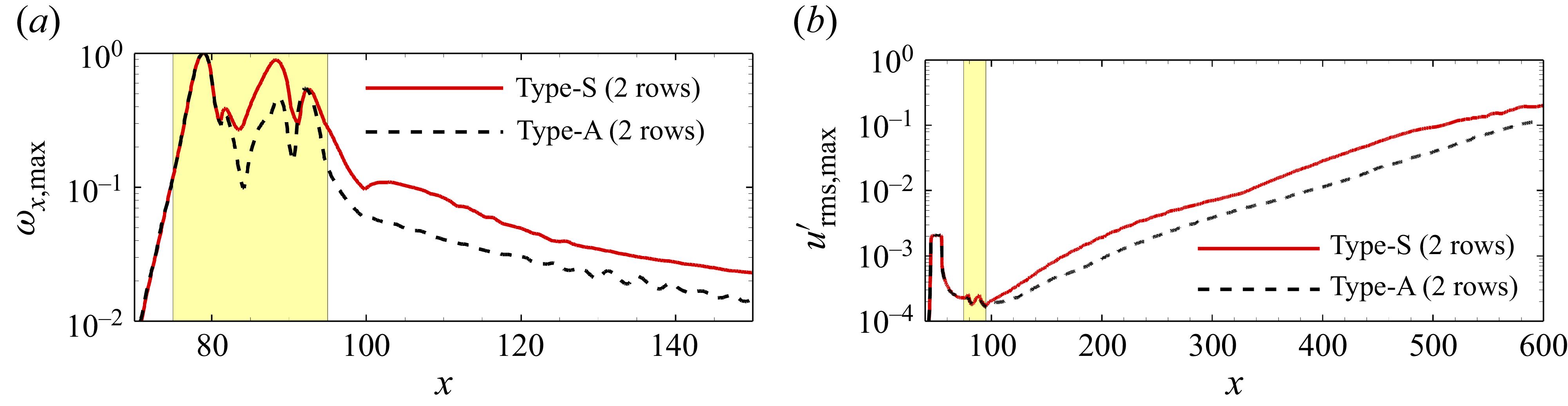
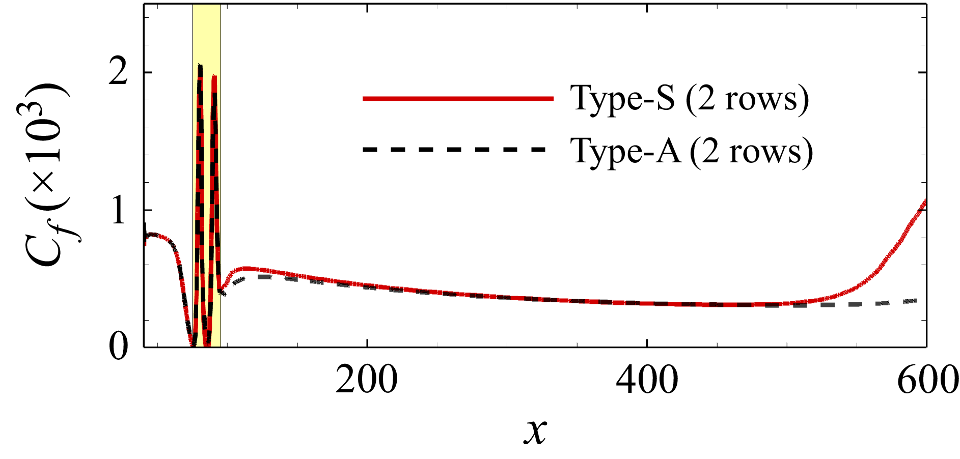
The differences between staggered and aligned distributions in affecting transition are examined when only two rows of roughness elements are present. The first two rows of the roughness elements in figure 2 are retained. Figure 36 shows the development of
 $\omega _{x,{max}}$
and
 $u_{\textit{rms}, {max}}^\prime$
along the streamwise direction for both staggered and aligned cases. It can be seen that
 $\omega _{x,{max}}$
in the type-S case is bigger than that of the type-A case, which indicates that the staggered-enhancing mechanism of streamwise vortices still exists for roughness with only two rows. This results in a faster growth of disturbances in the type-S case, as shown in figure 36(b). However, the difference between the type-S and type-A cases has decreased compared to the results with five rows in figures 11 and 20. To illustrate the transition process, figure 37 shows
 $C_f$
along the streamwise direction for two-row cases. It can be that the type-S roughness triggers transition near the end of the computational domain, while the flow remains laminar over the whole domain in type-A case. The transition onset positions in both two-row cases delay significantly compared to the five-row cases.
Developments of (a)
 $\omega _{x,{max}}$
and (b)
 $u_{\textit{rms},{max}}^\prime$
along the streamwise direction for roughnesses with two rows.

Time- and spanwise-average of
 $C_f$
for roughnesses with two rows.