1 Introduction
When looking around OECD countries, we see a variety of different pension system designs. Some of the systems are funded, many are unfunded, some of them are progressive, some of them are earnings related, see e.g., OECD (2011). Among the countries with earnings related pay-as-you-go (PAYG) systems, there basically exist two groups: the ones that calculate pension claims on the basis of some simple average of life time earnings (among them Germany, France, the USA, Canada, Belgium, Finland and Hungary)Footnote 1 and those who recently introduced so-called notional defined contribution (NDC) accounts (like e.g., Sweden, Italy, Poland and Norway). In the latter countries, contributions to the pension system earn a fictitious interest rate that is calculated from the sum of population growth and output growth per worker, see Auerbach and Lee (Reference Auerbach, Lee, Brown, Liebman and Wise2009). In the former, pension entitlements do not pay any (fictitious) interest at all.
In this paper, I argue that unfunded pension systems that follow the designs described above subsidize human capital formation. In an earnings related pension scheme such as the German system, contributions do not earn implicit returns. This creates an implicit tax because implicit savings in the pension system earn a lower return then explicit savings on the capital market. Due to compounded interest, this implicit tax is highest at the beginning of the working period and decreases over the life-cycle. This distorts the intra- and inter-temporal labor supply margin. As this paper shows, by use of a simple analytical model, this also distorts the human capital decision when there is a labor-leisure-education trade-off. As the costs for human capital accumulation are mainly time costs, the implicit tax structure reduces the costs of human capital formation and increases the benefits relative to a laissez-faire economy. This mechanism is reinforced by the steeper wage profile of college graduates. Obviously, the distortion is absent when implicit savings in the social security system are compounded with the ‘actuarially fair’ market interest rate. As a counterfactual I therefore analyze and quantify the macroeconomic and the welfare effects of switching from the current system to a system with actuarially fair implicit interest rates and therefore an age independent implicit tax structure. To this end, I build on the intuition from the simple model and develop a quantitative OLG model in the spirit of Auerbach and Kotlikoff (Reference Auerbach and Kotlikoff1987) with a discrete educational choice (college/non-college).
My simulations, which include full transitional dynamics, indicate that making the implicit tax structure of the pension system age independent has rather modest effects on the college enrollment decisions of households in the long run. The reason is that, if labor of different education types is not perfectly substitutable, the wage spread between unskilled and college workers increases, therefore bringing back people into college. However, the impact on on-the-job training is remarkable. There, human capital investments are reduced by 20 to up to 50%, depending on whether the economy is of closed or small open type. Labor supply declines by around 3% on average and partly shifts from high to low skilled labor. In the short run, however, when wages of different skill classes are not yet adjusted to the new situation, the number of college students decreases by roughly 2.5%. Short-run labor supply however increases, since fewer individuals participate in educational measures.
In terms of welfare, my reform comes along with a lot of intergenerational redistribution. Since labor supply increases in the short run and consumption taxes on the other hand decline, retirees that were already living in the initial equilibrium are the big winners from such a reform. Their welfare may increase by about 4.5% of their remaining life-time resources. Older workers, yet, are losing quite significantly, since under the old implicit tax structure their labor supply was subsidized, while under the new system it is taxed at about a 10% rate. Young generations, and especially the non-college population therein, gain from the reform, as the redistributive effect of the pension system toward college graduates is eliminated. In the long-run, however, this positive effect for the unskilled is almost mitigated through reactions in wages.
This paper stands in the tradition of examining questions of human capital formation in quantitative life-cycle models. Heckman et al. (Reference Heckman, Lochner and Taber1998) try to find an explanation for rising wage inequality between unskilled and skilled workers in the USA, whereas Guvenen et al. (Reference Guvenen, Kuruscu and Ozkan2013) explain pre-tax wage inequality between Europe and the USA through differences in progressive tax schedules. Abbott et al. (Reference Abbott, Gallipoli, Meghir and Violante2013) analyze alternative financial aid policies intended to promote college participation in partial and general equilibrium and show that additional government grants mainly crowd out intergenerational transfers from parents to children. Winter (Reference Winter2013) argues that such transfers are an integral determinant of the individual college choice. Caucutt et al. (Reference Caucutt, Imrohoroglu and Kumar2006) show that progressive taxation can have an impact on human capital formation and growth even when changes in flat rate taxes have none and that it may increase the long-run skill premium and decrease upward mobility of the poor. Finally, Krueger and Ludwig (Reference Krueger and Ludwig2013) study the optimal combination of a progressive tax schedule and educational subsidies in a general equilibrium model of overlapping generations in which human capital is formed through formal schooling. They find a progressive tax schedule in combination with a 70% subsidy of the resource cost of going to college to be the optimal policy.
Only few studies in the literature are however concerned with the impact of pension policy on human capital formation so far, among them Docquier and Paddison (Reference Docquier and Paddison2003) as well as Le Garrec (Reference Le Garrec2012), who analyze the growth and inequality effects of different pension arrangements in stylized overlapping generations models in which human capital is the engine of growth. They find that PAYG pension schemes have a negative effect on human capital formation. As they crowd out capital, the interest rate increases which makes human capital investments less valuable. However, Le Garrec (Reference Le Garrec2012) shows that pension systems can also enhance human capital formation, when pension benefits are only linked to the last years of earnings. He then states that there is a pension scheme which consists of a flat part and a part that is only related to the last years of employment, which leads to the same growth rate but less equality than a pure Bismarckian system. Another stream of the literature deals with the interaction between schooling, retirement and the pensions system. Lau and Poutvaara (Reference Lau and Poutvaara2006) find that increasing the link between pension benefits and contributions encourages human capital investment. Furthermore, actuarially adjusted arrangements like old-age benefits lead to later retirement compared to a retirement subsidy scheme and therefore prolong the period of yield for human capital investment. In consequence, schooling effort rises further, a result already found by Jensen et al. (Reference Jensen, Lau and Poutvaara2004) in a numerical study and confirmed by Montizaan et al. (Reference Montizaan, Cörvers and de Grip2010) in a quantitative study. Finally, Cascarico and Devillanova (Reference Cascarico and Devillanova2008) explore the consequences of funding social security in a model of human capital investment and capital skill complementarity in production. They state that the privatization of social security comes along with a higher steady state level of physical and human capital. As the capital stock increases, the wage gap between the skilled and the unskilled widens. Therefore across-group wage and income inequality rises.
The remainder of the paper is arranged as follows: In the next section I discuss the main effects of implicit taxes on household's college enrollment decisions in a simple analytical model. In Section 3 I then present my full numerical model, the calibration of which is shown in Section 4. Section 5 describes simulation results and the last section offers some concluding remarks.
2 A simple analytical model
Before going into the large scale numerical simulation model, I want to derive some intuition in a small analytical model. The focus of this analysis lies on the implicit tax structure inherent in earnings related PAYG pension systems and its effect on college enrollment decisions.Footnote 2
Lets assume that individuals live in overlapping generations for three periods and cohorts grow at the constant rate n period by period. In the first two periods they work, in the third they retire and live of their savings and some pension benefits p3. Furthermore let individuals be born with a certain educational ability s∼U([0,1]), which is uniformly distributed on the unit interval. Before starting to work in the first period, they have to choose whether to go to college or not. Let I(s) be an indicator function that takes value 1, if the agent of ability s goes to college, and zero otherwise. This model abstracts from leisure consumption. The net wage for an unskilled worker, i.e., someone that did not go to college, is w(1−τ), where τ is a contribution to the PAYG pension system. When going to college, a worker of ability s earns a wage premium πs in the first period of life and πsϵ2 in the second period, where ϵ2 ⩾ 1.Footnote 3 However, in order to receive this premium, an individual forgoes some time cost ϖ he could otherwise have worked as unskilled worker, i.e., the time cost of going to college is ϖw(1−τ). The dynamic budget constraints then read
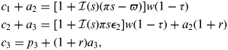 $$\eqalign{& c_1 + a_2 = [1 + {\rm {\cal I}}(s)(\pi s - \varpi )]w(1 - \tau ) \cr & c_2 + a_3 = [1 + {\rm {\cal I}}(s)\pi s\epsilon _2 ]w(1 - \tau ) + a_2 (1 + r) \cr & c_3 = p_3 + (1 + r)a_3,} $$
where r denotes the risk-free capital market interest rate.Footnote 4
Pension payments are indexed to the individual earnings history. Specifically, they are calculated as
 $$p_3 = \rho (r_p, n)\tau w\{ [1 + {\rm {\cal I}}(s)(\pi s - \varpi )](1 + r_p )^2 + [1 + {\rm {\cal I}}(s)\pi s\epsilon _2 ](1 + r_p )\}. $$
Thereby r p∊[0,r] is some (fictitious) return on pension contributions and ρ(r p,n) is the replacement parameter which is constant across s and in equilibrium will depend on the return factor r p as well as the population growth rate n. Note that τ is held constant throughout the whole analysis, i.e., the size of the pension system will not vary. The pension system operates on a PAYG basis, i.e., it collects contributions from workers and uses them to finance pension payments. Therefore
 $$N_3 \mathop \int \limits_{s \in [0,1]}\!\!\!\!\! p_3 \; ds = w\tau \left[ {N_1 \mathop \int \limits_{s \in [0,1]}\!\!\!\!\! 1 + {\rm {\cal I}}(s)(\pi s - \varpi )\; ds + N_2 \mathop \int \limits_{s \in [0,1]}\!\!\!\!\! 1 + {\rm {\cal I}}(s)\pi s\epsilon _2 \; ds} \right],$$
must hold in equilibrium, where N j denotes the population size of cohort j.
For simplicity the economy is assumed to be of small open type, i.e., factor prices are constant and the interest rate r equals the international capital market interest rate.
2.1 Solving for optimal college enrollment decisions
Using the dynamic budget constraints as well as the pension calculation formula (1), we can write the present value budget constraint of the household asFootnote 5
 $$\eqalign{c_1 + \displaystyle{{c_2} \over {1 + r}} + \displaystyle{{c_3} \over {(1 + r)^2}} = [1 + {\rm {\cal I}}(s)(\pi s - \varpi )]w[1 - \tau _1 (r_p, n)] + \displaystyle{{[1 + {\rm {\cal I}}(s)\pi s\epsilon _2 ]w[1 - \tau _2 (r_p, n)]} \over {1 + r}}$$
with
 $$\tau _1 (r_p, n) = \tau \left[ {1 - \rho (r_p, n) \cdot \left( {\displaystyle{{1 + r_p} \over {1 + r}}} \right)^2} \right]\quad {\rm and}\quad \tau _2 (r_p, n) = \tau \left[ {1 - \rho (r_p, n) \cdot \displaystyle{{1 + r_p} \over {1 + r}}} \right].$$
Thereby τ 1(r p,n) and τ 2(r p,n) denote the implicit tax rates of the pension system, see below. Under the assumptions of no leisure consumption and that households do not derive direct utility from education, the optimal choice of an individual of type s is to go to college only, if he gets higher income from that option than from directly joining the labor force as unskilled worker. Consequently, any individual for which
 $$\eqalign{[1 \!+\! \pi s - \varpi ]w[1 - \tau _1 (r_p, n)] + \displaystyle{{[1 + \pi s\epsilon _2 ]w[1 - \tau _2 (r_p, n)]} \over {1 + r}} \geqslant w[1 - \tau _1 (r_p, n)] + \displaystyle{{w[1 - \tau _2 (r_p, n)]} \over {1 + r}}$$
holds will decide to go to college. Note that the right-hand side of this equation is constant and the left-hand side is strictly increasing in s, as long as π>0. Therefore, there exists a unique s*∊[0,1] such that any individual with s⩾s* will go to college, everyone else will stay unskilled. The critical s* is defined by the equality
 $$\eqalign{\tab[1 + \pi s^* - \varpi ]w[1 - \tau _1 (r_p, n)] + \displaystyle{{[1 + \pi s^*\epsilon _2 ]w[1 - \tau _2 (r_p, n)]} \over {1 + r}} = w[1 - \tau _1 (r_p, n)] \cr\tab\quad+ \displaystyle{{w[1 - \tau _2 (r_p, n)]} \over {1 + r}}.$$
Solving for s* yields
 $$s^* = \displaystyle{{\varpi /\pi} \over {1 + \displaystyle{{\epsilon _2} \over {1 + r}} \cdot \displaystyle{{1 - \tau _2 (r_p, n)} \over {1 - \tau _1 (r_p, n)}}}}$$
Proposition 2.1
In the laissez-faire economy, we have
 $$s_{LF}^* = \displaystyle{{\varpi /\pi} \over {1 + \displaystyle{{\epsilon _2} \over {1 + r}}}}.$$
Proof. Setting τ = 0 yields 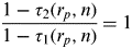 $\displaystyle{{1 - \tau _2 (r_p, n)} \over {1 - \tau _1 (r_p, n)}} = 1$ and therefore the critical level s* reported above.
In the laissez-faire case, the college enrollment decision depends on four parameters:
1. A higher ϖ increases the costs of education and therefore results in a lower amount of students (s LF*↑).
2. A higher college wage premium π increases the benefits of going to college and therefore has a positive effect on the number of students (s*↓). The same argument can be brought forward for an increase in ∊2.
3. The higher the interest rate r, the lower is the actualized return on education. Therefore, the number of students decreases with the interest rate (s*↑).
So far, this simple model behaves like any other model of human capital investment. The important part will then be to study the impact of the pension system on individual college enrollment behavior.
2.2 Internal rates of return in the pension system
Before analyzing the impact of implicit taxes on the college enrollment decision, let us first take a look at internal rates of return of the pension system. We can thereby distinguish between the average and the individual rate of return. The former is the interest rate i that equates the present value of aggregate pension contributions with the present value of aggregate pension benefits, the latter does this on an individual level.
Proposition 2.2
The average internal rate of return of the PAYG pension system i is independent of the accumulation rate rp.
Proof. Appendix A shows that the average internal rate of return of the pension system, i.e., the interest rate that equates the present value of aggregate pension payments with that of aggregate pension benefits, is i = n, regardless of the choice of r p, since by varying r p the replacement rate ρ(r p,n) adjusts accordingly in general equilibrium.
This is a well known and not surprising result. The rate of return of a pension system is equal to the so-called natural interest rate, i.e., the sum of population growth and the growth rate associated with technological progress. Since this model abstracts from technological progress, we get i = n. However, I will now show that this relation in general only holds on the aggregate level. On the individual level, internal rates of return between college educated and unskilled workers might actually differ.
Proposition 2.3. The individual internal rate of return of the PAYG pension system for the unskilled i nc is increasing in r p, given a constant college enrollment decision. Furthermore, the internal rate of return is constant over types and equal to n if i = 0 and ϵ2 = 1.
Proof. See Appendix A.
The above proposition tells us two things: first, pension systems with an accumulation rate r p lower than r come along with lower internal rates of return for the unskilled. Second this is only the case if there are either time costs of education or an additional wage premium for college educated workers in the second period of life. With these two Propositions in mind, we can now turn to analyzing the effect of implicit taxes on the college enrollment decision.
2.3 The impact of implicit taxes in the pension system on college enrollment
As mentioned above τ 1(r p,n) and τ 2(r p,n) denote the implicit tax rates of the pension system. One can interpret these tax rates in the following way: imagine that, instead of contributing a fraction τ of his income to the pension system, the household would save in the capital market in order to generate exactly the same income stream as the pension system in the retirement period. Taking period 1 as an example, for the contribution of  $\tau w[1 + {\rm {\cal I}}(s)(\pi s - \varpi )]$ the individual receives a pension income stream of
 $\rho (r_p, n)\tau w[1 + {\rm {\cal I}}(s)(\pi s - \varpi )](1 + r_p )^2 $ at retirement. In order to generate the same income through savings, the household would obviously have to invest the amount
 $\rho (r_p, n)\tau w[1 + {\rm {\cal I}}(s)(\pi s - \varpi )]\displaystyle{{(1 + r_p )^2} \over {(1 + r)^2}} $ in the capital market in the first period of live. Dividing this amount by the contribution to the pension system and multiplying it with the contribution rate yields the so-called implicit savings rate of the pension system
 $$\tau _1^s (r_p ) = \tau \cdot \displaystyle{{\rho (r_p, n)\tau w[1 + {\rm {\cal I}}(s)(\pi s - \varpi )]\displaystyle{{(1 + r_p )^2} \over {(1 + r)^2}}} \over {\tau w[1 + {\rm {\cal I}}(s)(\pi s - \varpi )]}} = \tau \rho (r_p, n)\displaystyle{{(1 + r_p )^2} \over {(1 + r)^2}}. $$
The implicit savings rate shows us what part of the pension contribution would actually have to be saved in the capital market, in order to generate exactly the same income stream as the pension system. Analogously, we can define the implicit tax rate as
 $$\tau _1 (r_p, n) = \tau - \tau _1^s (r_p ) = \tau \left[ {1 - \rho (r_p, n) \cdot \left( {\displaystyle{{1 + r_p} \over {1 + r}}} \right)^2} \right],$$
which is the same as the tax rate reported in equation (4). The implicit tax rate denotes the part of the contribution to the pension system that is perceived as a pure tax by the household.
There are two things to notice about the implicit tax rates. First, the population growth rate n only has an influence on the general size of implicit taxes, not on the evolution of implicit tax rates over the life cycle. We can see that by dividing
 $$\displaystyle{{\tau - \tau _1 (r_p, n)} \over {\tau - \tau _2 (r_p, n)}} = \displaystyle{{1 + r_p} \over {1 + r}},$$
which means that the evolution of implicit savings rates (the opposite of the tax rates) of the pension system over the life cycle is solely determined by the capital market interest rate as well as the accumulation factor r p. Furthermore, we can easily see that for r p<r we have
 $$\tau _1 (r_p, n) = \tau \left[ {1 - \rho (r_p, n) \cdot \left( {\displaystyle{{1 + r_p} \over {1 + r}}} \right)^2} \right] \gt \tau \left[ {1 - \rho (r_p, n) \cdot \displaystyle{{1 + r_p} \over {1 + r}}} \right] = \tau _2 (r_p, n),$$
as 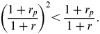 $\left( {\displaystyle{{1 + r_p} \over {1 + r}}} \right)^2 \lt \displaystyle{{1 + r_p} \over {1 + r}}.$ Therefore, as long as the accumulation factor r p is lower than the capital market interest rate, implicit tax rates in the PAYG pension system will be a decreasing function of age. In case of r p = r we obviously have τ 1(r p,n) = τ 2(r p,n). The next proposition formalizes the impact of this observation for college enrollment.
Proposition 2.4. For any PAYG pension system with rp < r, we have s rp*< s LF*. Only for r p = r we get s r* = s LF*.
Proof. We already saw above that
 $$\tau _1 (r_p, n) \gt \tau _2 (r_p, n)\;{\rm if}\;r_p \lt r\quad {\rm and}\quad \tau _1 (r_p, n) = \tau _2 (r_p, n)\;{\rm if}\;r_p = r.$$
From that it becomes immediately clear that s r* = s LF*. For r p < r we then have 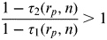 $\displaystyle{{1 - \tau _2 (r_p, n)} \over {1 - \tau _1 (r_p, n)}} \gt 1$ and therefore
 $1 + \displaystyle{{\epsilon _2} \over {1 + r}} \lt 1 + \displaystyle{{\epsilon _2} \over {1 + r}} \cdot \displaystyle{{1 - \tau _2 (r_p, n)} \over {1 - \tau _1 (r_p, n)}}$, which directly results in s rp* < s LF*.
Hence, pension systems under which pension claims are accumulated with an accumulation factor less than the capital market interest rate come along with a higher number of students. Therefore they distort the college enrollment decision compared to the laissez-faire case. The source of this distortion is twofold and can be much better interpreted by writing
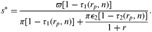 $$s^* = \displaystyle{{\varpi [1 - \tau _1 (r_p, n)]} \over {\pi [1 - \tau _1 (r_p, n)] + \displaystyle{{\pi \epsilon _2 [1 - \tau _2 (r_p, n)]} \over {1 + r}}}}.$$
In the numerator of this fraction we see the net opportunity cost of college education.Footnote 6 In the denominator the net present value of the wage premium. Lets assume for a moment that ∊2 = 1, i.e., there is no additional wage premium for college students in the second period of life. Then still we will find that s rp* < s LF* if r p < r. The reason for this is that the costs of college education are time costs, i.e., forgone earnings. By increasing implicit taxes in the first period and reducing them in the second, a pension system with r p < r subsidizes college education by reducing the net cost of college education and simultaneously increasing the payoff. A second effect comes into play when ∊2 > 1. In that case, increasing implicit tax rates in period 1 and decreasing them in period 2 not only subsidizes college education by lowering net time costs, but in addition through lowering tax rates during times in which the income of college educated workers is the highest. We therefore expect the college enrollment decision to respond more to changes in implicit tax rates and therefore r p when college students have a steeper wage profile than unskilled workers.
Summing up so far, we saw that pension systems with an accumulation rate of r p have an implicit tax structure with decreasing tax rates over the life cycle. As a direct result of this, such pension systems foster college enrollment and come along with lower internal rates of return for the unskilled population. The source of this distortion are both time costs of college education as well as the fact that college graduates might have steeper age-earnings profiles than unskilled workers. The next section discusses how to model different observed PAYG schemes around the world in my simple model and gives a numerical illustration.
2.4. Discussion and numerical illustration
As mentioned in the introduction, earnings related PAYG pension systems around the world can be divided into two groups: the ones that calculate pension claims on the basis of some simple average of life time earnings and those who recently introduced NDC accounts. In the latter countries, contributions to the pension system earn a fictitious interest rate that is calculated from the sum of population growth and output growth per worker. In my simple model, we can characterize these two different systems by setting r p = 0 for a simple life time earnings average and r p=n for NDC accounts. However, none of the PAYG systems has an accumulation rate of r p = r.
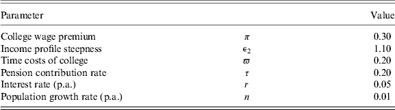
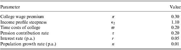
In order to get a first idea about how the key variables in this simple model evolve when we change r p, I parameterize the model with the calibration shown in Table 1 and simulate the model for different values of r p∊[0,0.05] (in p.a. terms). The parameters I use are fairly standard. Note that in a three period model a period covers roughly 25 years, so time costs of ϖ = 0.20 means that individuals have to attend college for about 5 years.
Calibration of the simple model
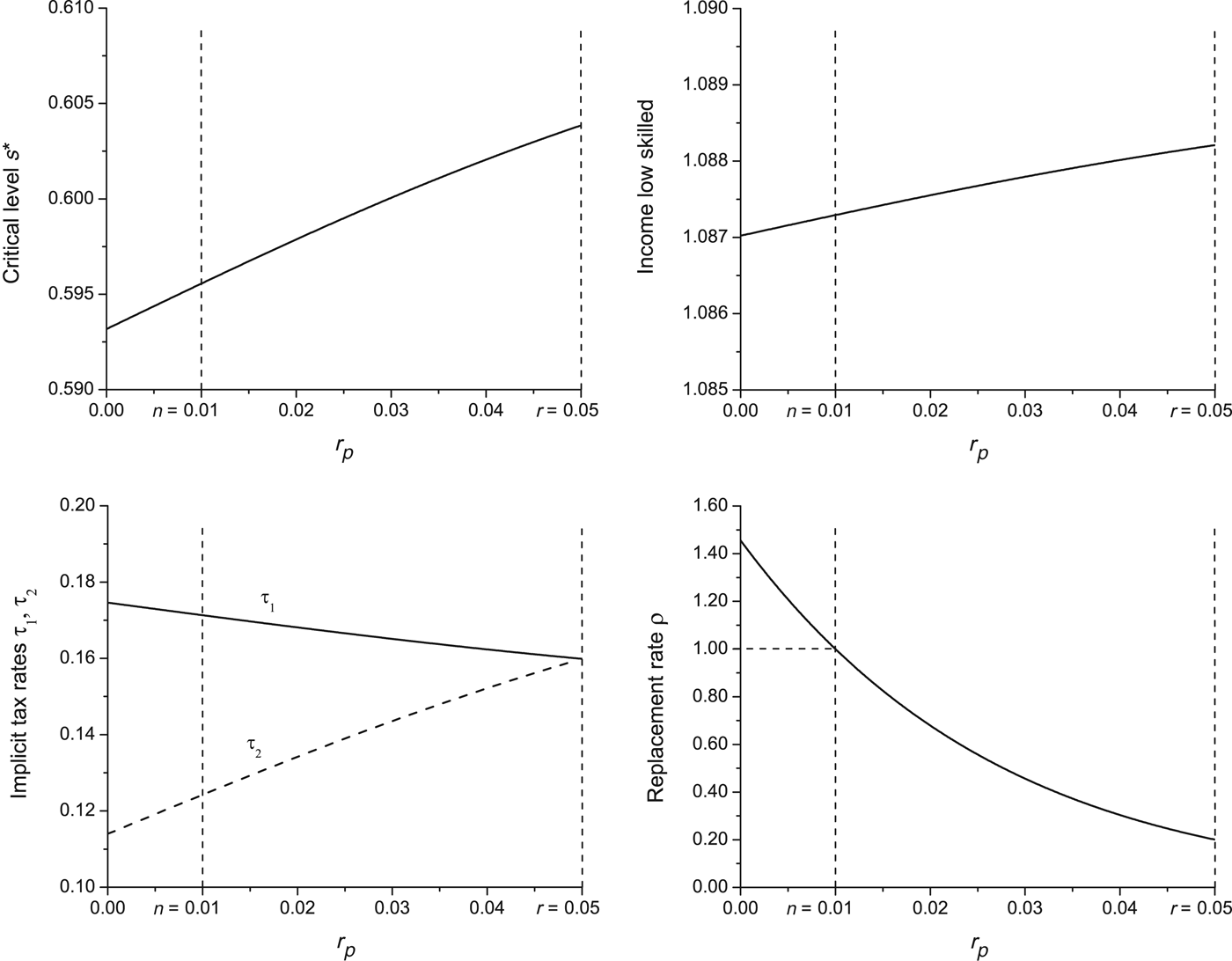
The model results for different values of r p are shown in Figure 1. First we can see that for low values of r p, the critical s* is about 1% point lower than for r p = r (which corresponds to the laissez-faire case). The upper right panel then shows the implicit tax rates. As described above, for r p = r we have τ 1 = τ 2. As r p becomes smaller and smaller, the wedge between the two tax rates increases significantly, so that at r p = 0 it amounts to roughly 6% points. In the lower right panel, we can see how the replacement rate adjusts with r p. Since L 1(1 + r p)2 + L 2(1 + r p) increases drastically with r p, the replacement rate adjusts downwards as I increase the accumulation factor. Note that, as we have already seen above, this does not have an impact on the average internal rate of return of the pension system. However, the effect on the internal rate of return of the unskilled can finally be seen in the upper right panel of Figure 1. As the internal rate of return increases with r p, it is clear that also income of the lower skilled has to increase, since the timing of their income does not change with r p.
Results of the simple model.

All in all we can see from this simple simulation, that pension systems with an accumulation factor of r p < r distort the college choice of households, such that more individuals decide to attend college. Furthermore, these systems redistribute from the unskilled toward the skilled. However, the numbers reported here are only a very rough approximation of what would happen in an economy, when we alter the accumulation factor of the pension system. Furthermore, factor price movements have been completely neglected up to now. To get a better insight into how important the distortion of human capital accumulation may be and into what would happen in the short and long run, if we reformed the pension system by introducing an accumulation factor of r p = r, I now construct a large scale OLG general equilibrium model. The model features two mechanisms of human capital formation: going to college and on-the-job training. Furthermore, in the following sections, I will not only compare long-run equilibria, as I did in this section, but calculate full transition paths that arise from reforming the pension system. This allows me to study both short and long run welfare effects of a pension reform.
3 The numerical general equilibrium model
I use a model of overlapping generations in the tradition of Heckman et al. (Reference Heckman, Lochner and Taber1998) to quantify the impact an earnings related PAYG pension system has on human capital formation as well as the macroeconomy and welfare of different generations. The model features three sectors: households, firms and the government. In this section, I provide information about the decision rules for these different actors. This model description follows closely the one in Kindermann (Reference Kindermann2012). Detailed descriptions of a general equilibrium path and computational methods can also be found there.
3.1 Demographics, endowments and intra-cohort heterogeneity
The model economy is populated by J overlapping generations. At each point t∊{0,1,…,∞} in time a new generation is born, where successive cohorts grow at rate n, i.e., N 1,t = (1 + n)N 1,t −1. From one date to the other a fraction of agents of each cohort dies. Let ψ j ⩽ 1 be the conditional survival probability to age j of an agent aged j − 1. Then
 $$N_{\,j,t} = \psi _j N_{\,j - 1,t - 1}, $$
holds with N j,t being the size of the age j cohort at time t. At the beginning of their life-cycle, households are born with some exogenous educational ability s p. Households are assigned to an ability level according to the probability function F(s p). Individuals start their life with zero assets a 1 = 0, an identical amount of human capital  $\bar h_1 $ and the educational level s 1 = 1.
At any age during their life, I can distinguish different agents according to their individual state vector
 $$z_j = (s_p, s_j, a_j, m_j, h_j ).$$
s p∊S = {1,…,S} denotes agent's ability and s j∊S his education level. a j∊A = [0,∞), m j∊P = [0,∞) and h j∊H = [0,∞) describe asset holdings, pension entitlements and household's human capital level, respectively. For simplicity reasons I will omit the time index t in the following, whenever possible.
3.2 The decision problem of individuals
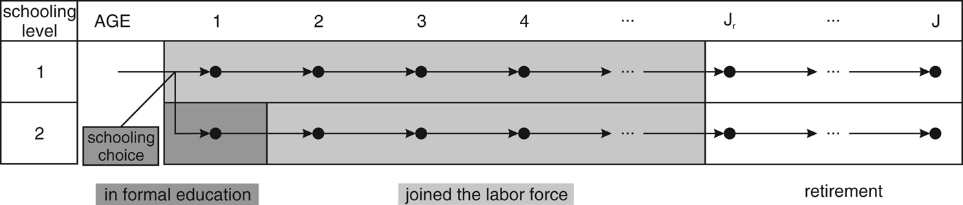
I divide households’ life-cycle into three distinct stages. Agents start making economically relevant decisions by the age of j = 1 at which they have to decide whether to enroll in college/universityFootnote 7 or directly join the labor force. There consequently are two different education levels: secondary education (s = 1) and tertiary education, i.e., a college/university degree (s = 2). When agents decide to drop-out of the educational sector and join the labor force, this decision is irreversible. Having joined the labor force, individuals may still increase their human capital h j by means of on-the-job training. In addition, they supply labor to the market and enjoy leisure consumption. Finally, every individual has to retire at the mandatory retirement age J r. Figure 2 sketches the life-cycle of households.
The life-cycle of households.
Agents value consumption streams according to the expected utility functionFootnote 8
 $$E\left[ {\mathop \sum \limits_{\,j = 1}^J \beta ^{\,j - 1} u(c_j, \ell _j )} \right],$$
where c j and  $\ell _j $ denote goods and leisure consumption and β is a time discount factor. The instantaneous utility function u satisfies the usual conditions
 $\displaystyle{{\partial u} \over {\partial c_j}}, \displaystyle{{\partial u} \over {\partial \ell _j}} \gt 0$ and
 $\displaystyle{{\partial ^2 u} \over {\partial c_j^2}}, \displaystyle{{\partial ^2 u} \over {\partial \ell _j^2}} \leqslant 0$. Due to the additive separability of utility with respect to age, I can formulate the individual maximization problem in recursive form.
3.2.1 The retirement phase
Households in the retirement phase use their assets a j and pension claims p j to finance consumption c j. Furthermore, they consume their maximum time endowment of 1 as leisure. Their maximization problem is
 $$V_j (z_j ) = \mathop {\max} \limits_{c_j, a_{\,j + 1}} u(c_j, 1) + \beta \psi _{\,j + 1} V_{\,j + 1} (z_{\,j + 1} ),$$
with V j denoting household's value function at age j. The only risk agents face during retirement is survival to the next period j+1.Footnote 9
Individuals maximize their utility subject to the budget constraint
 $$a_{\,j + 1} + (1 + \tau _c )c_j = [1 + r(1 - \tau _r )]a_j + p_j + b_j, $$
where a j denotes asset holdings at the beginning of the period. In addition to after tax interest income from savings (1−τ r)ra j, households receive pension benefits p j and accidental bequests b j. Note that neither income from pensions nor from bequests is due to taxation. The price of the consumption good already contains the consumption tax rate τ c. By assumption, households are liquidity constrained throughout their whole life, i.e., a j⩾0 must hold at each j.
Pension claims are indexed to wages. They are calculated as the product of a replacement rate ρ, pension entitlements that were accumulated up to retirement age m Jr (see below) and average labor income of working households  $\bar y_t $ at time t
 $$p_j = \rho \cdot m_{J_r} \cdot \bar y_t. $$
3.2.2 Working agents
Once having joined the labor force, households must decide on how to divide their time endowment between labor supply l j, leisure consumption  $\ell _j $ and on-the-job training e j. With the latter of these they can influence their future human capital h j+1. They consequently have to solve the maximization problem
 $$V_j (z_j ) = \mathop {\max} \limits_{c_j, \ell _j, e_j, a_{\,j + 1}, h_{\,j + 1}} u(c_j, \ell _j ) + \beta \psi _{\,j + 1} V_{\,j + 1} (z_{\,j + 1} ),$$
subject to the budget constraint
 $$\eqalign{a_{\,j + 1} + (1 + \tau _c )c_j + \kappa _j + \vartheta _j = \left[ {1 + r(1 - \tau _r )} \right]a_j + (1 - \tau _w )y_j - \tau _p \min {\rm \;} (y_j, \varsigma \cdot \bar y) + b_j. $$
Individuals receive income from working in the market
 $$y_j = w_{s_j} \cdot h_j \cdot l_j, $$
which is the product of the education specific wage rate  $w_{s_j} $, labor productivity h j and labor supply
 $l_j = 1 - \ell _j - e_j $. In addition to paying taxes on labor and interest income, they have to contribute at the flat rate τ p to the pension system, where the pension system only covers income below a cap of ς times the average labor income. Beyond financing consumption and savings, agents use their net income to give intergenerational transfers κ j to their children and repay their debt out of a governmental student loan scheme
 $\vartheta _j $. The size of intergenerational transfers is exogenously determined.
In reward for their contribution to the pension system, households accumulate pension claims in proportion to their labor income. Pension claims evolve according to
 $$m_{\,j + 1} = \left[ {m_j + \min {\rm \;} \left( {\displaystyle{{y_j} \over {\bar y_t}}, \varsigma} \right)} \right] \cdot (1 + r_p ),$$
where r p again denotes the accumulation factor. Note that the amount of pension entitlements only depends on the relative income position of a household in the economy at date t. Furthermore, in line with the German practice, one only accumulates pension entitlements on the basis of income below the contribution limit  $\varsigma \bar y$. Therefore, the same cap applies in the accumulation formula for pensions.
Should an agent drop out of the schooling system his education level persists over the rest of his life, i.e., s j+1=s j. However, he can still influence his human capital by investing on-the-job. I assume that time e j is the only cost of on-the-job training and let human capital develop according to
 $$h_{\,j + 1} = A_s e_j^{\alpha _s} + h_j. $$
The human capital production function therefore is a special case of the function proposed in Heckman (Reference Heckman and Terleckyj1976). Note that the ability parameter A s and the elasticity of additional human capital with respect to time input α s only depend on the agent's education level.Footnote 10
3.3 College education
The college education technology differs from on-the-job training: when in college, individuals have to devote a certain fraction  $\varpi _{s_p} $ of their time endowment to studying, which depends on their ability level s p. In reward for this time, they receive an (exogenous) level of human capital
 $\bar h_2 $ after having graduated successfully. With this human capital they enter the labor force in the next period of life. Households make their college enrollment decision via a comparison of utilities at the beginning of period 1. As they all start out with zero assets and pension claims as well as an identical level of human capital
 $\bar h_1 $, their value functions reduce to
 $$W_1 (s_p ) = V_1 (s_p, 1,0,0,\bar h_1 )\quad {\rm and}\quad W_2 (s_p ) = V_1 (s_p, 2,0,0,\bar h_1 )$$
in the cases they directly join the labor force and attend university, respectively. An individual of ability type s p will then choose to enroll in college, if
 $$W_2 (s_p ) + \varepsilon \geqslant W_1 (s_p ).$$
Similar to Willis and Rosen (Reference Willis and Rosen1979) and Heckman et al. (Reference Heckman, Lochner and Taber1998), I capture unobservable characteristics by means of ‘non-pecuniary costs of college education’ ε, where ε is normally distributed with mean 0 and variance σ ε2.Footnote 11 I assume that there is a large amount of individuals in each ability group and let the random variables ε for different states be stochastically independent. Then
 $$P\left\{ {W_2 (s_p ) + \varepsilon \geqslant W_1 (s_p )} \right\} = 1 - N_{0,\sigma _\varepsilon ^2} \left[ {W_1 (s_p ) - W_2 (s_p )} \right] = d(s_p ),$$
is the fraction of individuals of ability s p who decide to attend university.
College students can split their remaining available time  $1 - \varpi _{s_p} $ that is not devoted to studying between consuming leisure and supplying labor to the market. Leisure consumption then amounts to
 $\ell _j = 1 - \varpi _{s_p} - l_j $. In addition, they receive transfers κ j from their parents and payments
 $\vartheta _j $ out of a governmental student loan scheme. They again use their net income to finance consumption expenditure and to possibly build up some assets.
3.4 Intergenerational transfers
Evidence in Eckstein and Wolpin (Reference Eckstein and Wolpin1999), Cingano and Cipollone (Reference Cingano and Cipollone2007) as well as Carneiro and Heckman (Reference Carneiro and Heckman2002) shows that the ability to form human capital via formal schooling depends strongly on the education level of the parents. Due to a lack of data on individual ability, I therefore assume that there are only two ability types s p in the population and that ability is perfectly identified by the education level of the parents. Consequently, one can interpret s p as the parental background of an individual. In order to link generations, I let parents be of age J p when children enter their economically relevant phase of life. Unlike Abbott et al. (Reference Abbott, Gallipoli, Meghir and Violante2013), Winter (Reference Winter2013) or Krueger and Ludwig (Reference Krueger and Ludwig2013) I do not assume parents to be altruistic toward their children in a dynastic sense. This ensures that I do not run into the problem of Ricardian equivalence. Instead I let transfers between generations κ j be exogenous and conditional on parents' education level.Footnote 12 Specifically, I set
 $$\kappa _1 (z_1 ) = \kappa _{s_p} \quad {\rm if}\quad z_1 = (s_p, 2,1,0,0,\bar h_1 ),$$
i.e., children only receive transfers from their parents during formal education. Of course, the sum of lump-sum transfers to children must be financed by the parent generation.
Since annuity markets are absent in this model, private assets of all agents who died are aggregated and then distributed among all working age cohorts following an age-dependent distribution scheme. The distribution of bequests is computed in every period, where I assume that children always inherit assets of their parents' generation j p. Since bequest can only be received during employment, I adjust this rule at the beginning and the end of the employment phase. In order to account for agents’ parental background, within each cohort, the distribution is computed such that households with background s p receive assets from agents of schooling type s jp = s p of the parental generation. Among individuals of a cohort and socio-economic background, bequests are then distributed equally. As the more educated usually are the more wealthy, households with richer parents will receive more bequests than those with poorer socio-economic background.
3.5 Firms behavior
A continuum of firms produce under perfect competition with the Cobb–Douglas technology
 $$Y = {\rm \Lambda} \cdot K^{\chi _1} \cdot L^{1 - \chi _1}. $$
In line with Katz and Murphy (Reference Katz and Murphy1992), I compute aggregate labor input in production from
 $$L = \left\{ {\lambda _1 L_1^{1 - \textstyle{1 \over {\chi _2}}} + \lambda _2 L_2^{1 - \textstyle{1 \over {\chi _2}}}} \right\}^{\textstyle{1 \over {1 - \textstyle{1 \over {\chi _2}}}}}. $$
For χ 2<∞, labor of different educational types is therefore not perfectly substitutable. Firms maximize output net of labor and capital costs. Capital costs include a constant depreciation rate of δ k. Due to the assumption of perfect competition, factor prices equal net marginal products, i.e.,
 $$r = \displaystyle{{\partial Y} \over {\partial K}} - \delta _k \quad {\rm and}\quad w_s = \displaystyle{{\partial Y} \over {\partial L_s}}. $$
3.6 The government
The government runs two systems with separate budgets: a tax and a pension system.
The tax system collects taxes on consumption C, labor income w 1L 1 + w 2L 2 and capital income rA in order to finance expenditure on public consumption G and on education G s as well as interest payments on existing debt rB. The costs associated with education level s consist of two components: a fixed cost per student g s (provision costs) and possible burdens arising from the student loan system  $\vartheta _j $.Footnote 13 Income taxes are levied at proportional rates τ w and τ r. Government debt is held constant per capita of the population and the consumption tax rate balances the government's budget on a period by period basis. The tax system's budget then reads
 $$\tau _c C + \tau _w [w_1 L_1 + w_2 L_2 ] + \tau _r rA = G + G_1 + G_2 + (r - n)B.$$
I assume that government debt is held constant per capita over time. The consumption tax rate balances the government's budget periodically.
The pension system runs on a PAYG basis. In every year, it collects contributions at the flat rate τ p in order to finance pension payments to existing retirees, i.e., its budget constraint reads
 $$\tau _p [w_1 L_1 + w_2 L_2 ] = P,$$
where P denotes aggregate pension benefits. The replacement rate ρ balances the budget of the pension system on a period by period basis.
3.7 General equilibrium
Given a specific fiscal policy, a competitive equilibrium path of the economy is a set of competitive factor prices, budget clearing tax rates and stocks of debt as well as household decision rules that satisfy the following conditions:
1. The capital market clears, i.e.,
(22) $$A_t = K_t + B_t. $$
2. Labor demand of the firms for the two educational levels equals labor supply.
3. The goods market clears, i.e.,
(23)$$Y_t = C_t + G_t + G_{1,t} + G_{2,t} + (1 + n)K_{t + 1} - (1 - \delta _k )K_t. $$


A long-run equilibrium is an equilibrium path on which aggregate variables grow at constant rate n and per capita variables are constant over time.
4 Calibration strategy
I use a combined estimation and calibration strategy with German data that is very much in line with Kindermann (Reference Kindermann2012) to parameterize my model. Specifically, I
1. specify demographic and educational parameters;
2. estimate hourly wage profiles from socio-economic panel (SOEP) panel data;
3. use these wage profiles to determine the parameters of on-the-job training via a method of moments estimator;
4. set the parameters that determine college choices;
5. calibrate the remaining model parameters.
4.1 Demographics, educational levels and the distribution of bequests
I let one model period cover 5 years for computational reasons. Agents start making economically relevant decisions by the age of 20 (j = 1), are 45 when their children turn 20 (J p = 6), retire at age 60 (J R = 9) and live up to a maximum of 100 years (J = 16). The college enrollment decision therefore has to be taken at age 20, which is line with the German educational system. I classify education levels according to the ISCED 1997 Standard issued by UNESCO (2006). I merge levels 0–4 (secondary education) and 5 and 6 (tertiary education) to obtain the two education levels. I furthermore assume that the distribution F(s p) mimics the current education status of the population. OECD (2010) reports that currently about 25% of the adult population between ages 35 and 54 hold a tertiary education degree. I therefore set F(s p = 1) = 0.75 and F(s p = 2) = 0.25.
Individual survival probabilities are taken from Bomsdorf (Reference Bomsdorf2002) and population grows at 1% per year, i.e., n = 0.05.Footnote 14 As for the distribution of unintended bequests, I assume children to inherit the assets of their parents. Therefore, children with higher educated parents (s p = 2) will receive a larger amount of bequest and households at ages j > J − J p do not receive any, since their parents are already dead with certainty.
4.2 Human capital production on-the-job
I use data of the German SOEP to estimate hourly wage profiles. Specifically, I calculate deflated hourly wages h i,j,t,s of individuals i at age j and time t and classify them according to the two education levels s mentioned above. Self-employed, interns and civil servants are excluded from my data set, since they tend to have quite different wage dynamics. In addition, I exclude the upper and the lower percentile of the hourly wage distribution in order to rule out errors in the data.
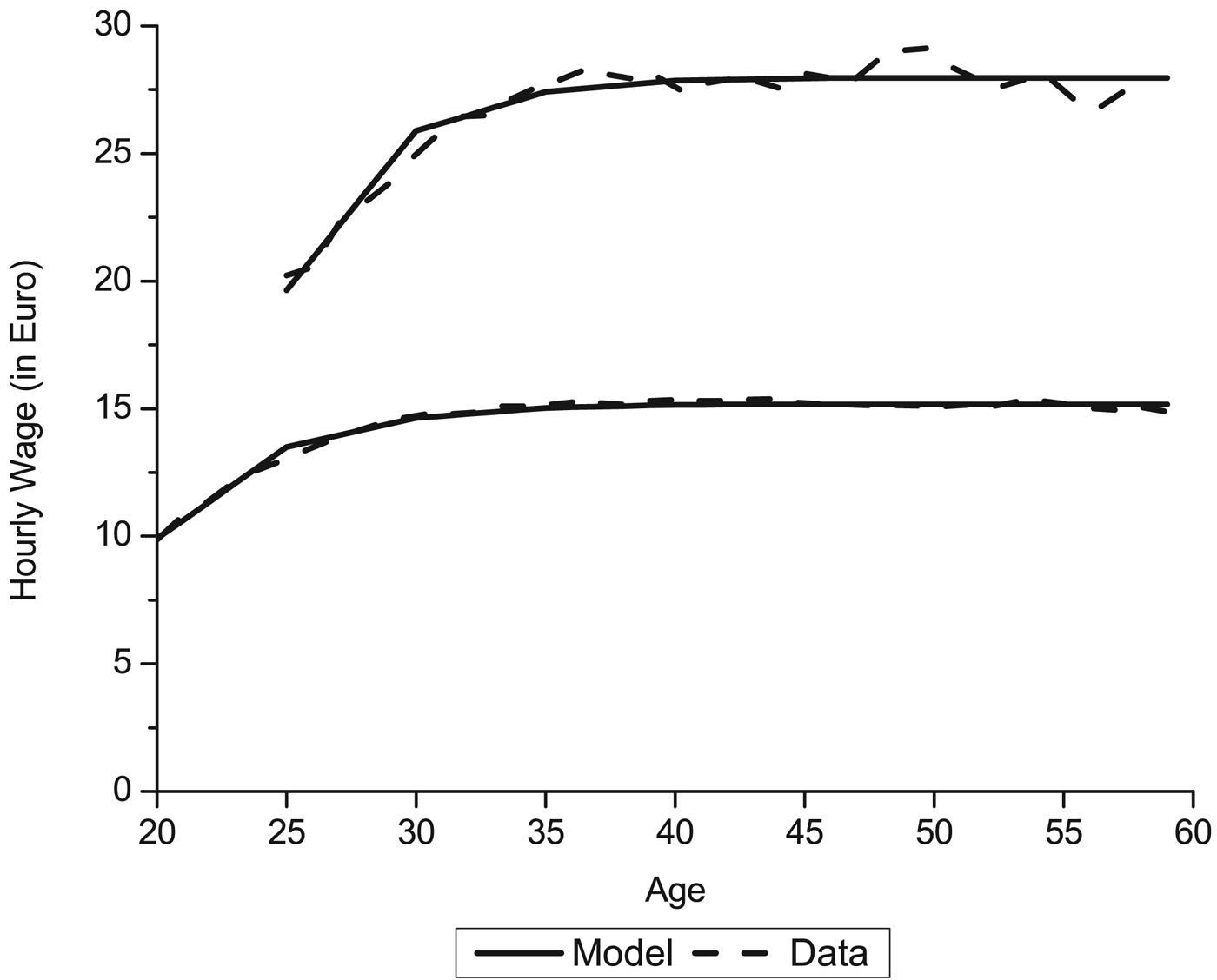
I then apply the method described in Kindermann (Reference Kindermann2012) to determine the human capital production functions for individuals of different educational levels. I first estimate an age- and year fixed effect regression. I then use the age fixed effects to determine human capital production functions via a partial equilibrium method of moments estimation. The results of this process are shown in Table 2 and Figure 3.
Hourly wage profiles for different education levels.
Estimation results for human capital production on-the-job

4.3 College choice
Table 3 shows the parameters determining household's college enrollment decision. The annual transfers in Euro from the government and from parents to their children during college attendance are taken from Autorengruppe Bildungsberichterstattung(AB) (2008). Note that households have to repay half of the transfers they received from the government without interest starting 5 years after they left university. This is in line with the German practice.
Determinants of the college enrollment decision

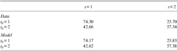
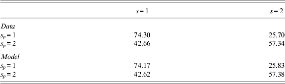
Having set monetary transfers, I calibrate time costs of studying in order to replicate participation rates reported in Heineck and Riphahn (Reference Heineck and Riphahn2009). Note that time costs of studying do not necessarily reflect pure time efforts. They might also incorporate ‘mental studying costs’, since I assumed unobservable characteristics ε s to have zero mean. Finally, I set the variance σ ε2 = 0.00514 which is in line with the estimates of Heckman et al. (Reference Heckman, Lochner and Taber1998). Table 4 reports participation rates computed from Heineck and Riphahn (Reference Heineck and Riphahn2009) as well as my model generated data.
Participation rates by socio-economic background
4.4 Household preferences, production technology and the government
Household preferences
I let instantaneous utility be represented by the constant relative risk aversion utility function
 $$u(c,\ell ) = \displaystyle{1 \over {1 - \gamma}} [c^{1 - \nu} + \mu \ell ^{1 - \nu} ]^{\textstyle{{1 - \gamma} \over {1 - \nu}}}, $$
γ denotes risk aversion and ν the inverse of the elasticity of substitution between consumption and leisure. μ is a measure for leisure preference. I choose a fairly standard risk aversion of 2 which implies an intertemporal elasticity of substitution of 0.5. ν is set to 1.7 leading to an aggregate Frisch elasticity of labor supply of 1.14, which corresponds to the values reported in the literature, see e.g., Ludwig et al. (Reference Ludwig, Schelkle and Vogel2011).Footnote 15 I calibrate μ to 0.8. This causes the average of working hours to amount to 31.6%, which is in line with the data reported in Institute der Deutschen Wirtschaft (IW) (2011). Finally, I set the time discount factor at β = 0.93. This choice corresponds to a 1.4% annual time discount rate and leads to a capital to output ratio of 3.5. IW (2011) reports a value of 3.5 for 2010.
Production technology
In the production sector I let χ 1 = 0.35, which guarantees a labor income share of 0.65. I then take the elasticity of substitution between labor of different types from Heckman et al. (Reference Heckman, Lochner and Taber1998) (χ 2 = 1.41) and calibrate the labor shares λ s so as to receive the same wage rate for effective labor for both skill classes. A technology level of Λ = 0.13 ensures wage rates to be normalized to unity. Finally, I assume an annual depreciation rate of capital of 4.5% which leads to an investment level of 19.3% of GDP.
The government
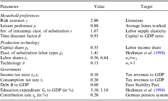
I calibrate consumption and income tax rates so as to match tax revenues from these sources reported in IW (2011). This leads to τ c = 0.20 and a uniform income tax of τ w = τ r = 0.10. I let government debt be 60% of GDP in the initial equilibrium, which is the long-term target of the European Stability Pact, and set public expenditure on different educational levels G s to the values reported in OECD (2009). In the pension system, I set the replacement rate ρ to an amount that generates a contribution rate of 20%, which is close to the current contribution rate of the German pension system. The accumulation factor is set to r p = 0 like in the German pension system. Current statistics in Deutsche Rentenversicherung Bund (2012) show that the contribution limit varied in the last years around a value of roughly 2–2.1 times the average labor income. I therefore choose ς = 2. Table 5 summarizes calibrated parameter values and their targets.
Calibrated model parameters and their targets
5 Simulation results
In this chapter, I present evidence on how my model performs in replicating German macroeconomic data. I then describe how I implement policy reforms. The remainder of the chapter is dedicated to policy analyses.
5.1 The initial equilibrium
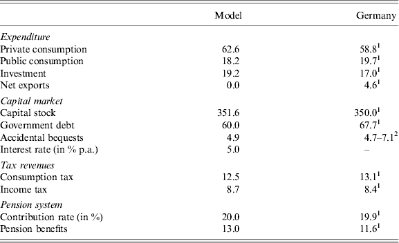
All my simulations start from an initial long-run equilibrium that replicates selected macroeconomic facts of the German economy. Table 6 compares model generated macro data with their real equivalents in Germany in 2010. Since I assume a closed economy setting and Germany is a net exporter, private consumption is higher than in reality. Public consumption, on the other hand, is a little too low. This is because the government issues less new debt than in reality. Overall I find that my model reasonably replicates German macroeconomic indicators.
Macro data in initial equilibrium (in % of GDP)
Source: 1IW (2011), 2Braun et al. (Reference Braun, Burger, Miegel, Pfeiffer and Schul2002).
5.2 Thought experiment
We now want to study how the introduction of an accumulation factor that equals the (net) capital market interest rate r p,t = r t(1 − τ r) influences the individual propensity to invest in human capital as well as the macroeconomy and welfare of different generations. I therefore simulate a counterfactual starting from the initial equilibrium (t = 0) reported above. In period t = 1 of the transition I introduce an accumulation factor for pension claims r p,t = r t(1 − τ r). Pension entitlements that were accumulated in the initial equilibrium will be fictitiously recalculated as if they were accumulated under the new scheme with positive accumulation factor.Footnote 16 I then simulate a full transition path toward a new long-run equilibrium. I thereby assume that the contribution rate τ is fixed and that the replacement rate ρ balances the budget on a period by period basis.
In order to understand the effects triggered by the reform, it is crucial to know the implicit tax structure of the pension system in this large scale model. Again this is fairly easy to calculate. Like in the simple model, we have to find out what an individual at age j would have to save in the capital market in order to generate exactly the same income stream as the pension system and relate this to the contribution he makes. In steady state, the pension contribution of an individual of age j is equal to τ·y j. In reward for this contribution, he receives a pension of  $\rho \bar y(1 + r_p )^{J_r - j} $ between the ages J r and J.Footnote 17 The present value as of age j of this pension income stream is
 $$\rho y_j (1 + r_p )^{J_r - j} \cdot \mathop \sum \limits_{i = J_r} ^J (1 + r(1 - \tau _r ))^{\,j - i} = \rho y_j \left( {\displaystyle{{1 + r_p} \over {1 + r(1 - \tau _r )}}} \right)^{J_r - j} \cdot \mathop \sum \limits_{i = J_r} ^J (1 + r(1 - \tau _r ))^{J_r - i}. $$
In full analogy to the small model, relating this to the pension contribution and multiplying it with τ yields the implicit savings rate
 $$\tau _j^s = \rho \left( {\displaystyle{{1 + r_p} \over {1 + r(1 - \tau _r )}}} \right)^{J_r - j} \cdot \mathop \sum \limits_{i = J_r} ^J (1 + r(1 - \tau _r ))^{J_r - i}. $$
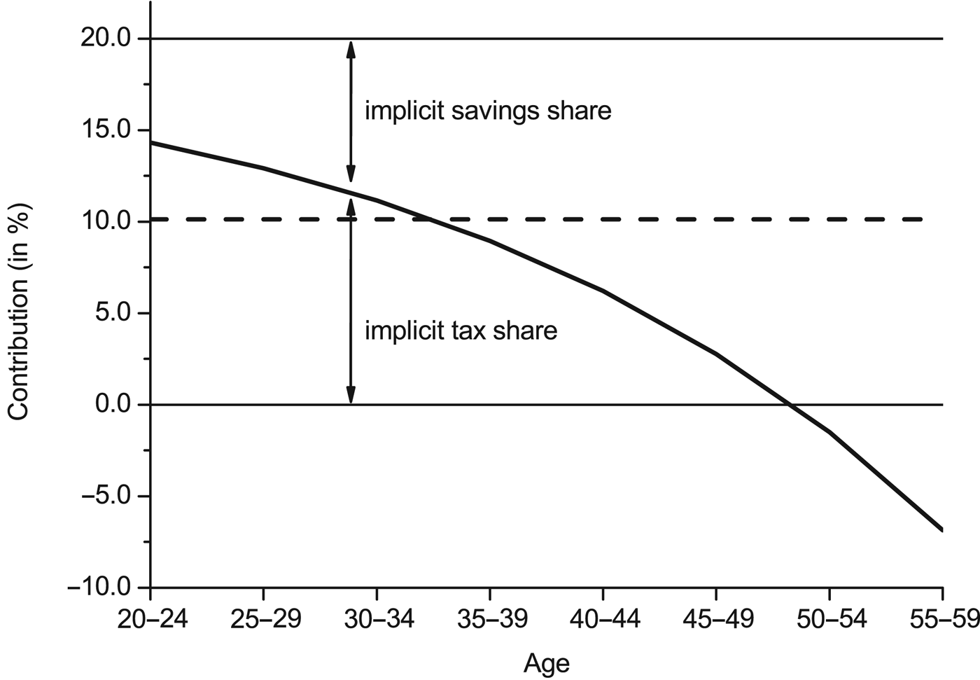
The implicit tax rate then again is given by τ j = τ−τ js. Obviously, the evolution of the implicit tax rate depends crucially on the interest rate r and the accumulation rate r p. Figure 4 shows implicit tax rates in the case of r p = 0 (solid line) and r p,t = r t(1−τ r) (dashed line), i.e., in the initial and the new long-run equilibrium.
Implicit savings and tax components of pension contributions.
We directly see that in the case of r p = 0 we again have a decreasing implicit tax structure. Toward the end of working life, these implicit tax rates even turn significantly negative, which means that the pension system actually subsidizes labor supply in these periods. In the case of r p,t = r t(1−τ r), the tax structure is completely flat over the life cycle.
But what do we expect from introducing an accumulation factor equal to the net capital market interest rate? First of all, as we have learned from the simple model, the number of students should reduce in the long run from such a reform. But there is more to it in this larger model. In terms of on-the-job training, the same reasoning applies. Since the costs of this investment are pure time costs, we again expect a decreasing implicit tax structure to foster on-the-job training efforts in the same way as college enrollment. Consequently, from introducing a positive accumulation factor, on-the-job training efforts should also decrease in the long-run. Last but not least, the implicit tax structure will also have a significant effect on labor supply. In the case of a decreasing implicit tax structure, labor supply near the end of the working phase will be subsidized. This certainly increases hours worked and therefore the rental rate of human capital investment (especially that of on-the-job training). When we go over to a flat structure by setting r p,t = r t(1−τ r), this subsidizing effect is gone and will be replaced by a distortion. Consequently, the return on human capital investment decreases and the decline in both study enrollment rates and on-the-job training effort will be enforced. Summing up, we can form the following three hypothesis: the introduction of an accumulation factor of r p = r(1−τ n) will
1. come along with a decline in the number of students and
2. a reduction in on-the-job training efforts;
3. have stronger effects when leisure consumption (and therefore labor supply) is endogenous.
In the following I want to test these hypotheses in my model.
5.3 Simulation results: exogenous vs. endogenous leisure consumption
In order to be able to test the above hypotheses, I will start with a small open economy setting and let labor of different educational levels be perfectly substitutable (χ 2 = ∞). Therefore, factor prices will remain unchanged along the transition path and in the new long-run equilibrium. I then consider two different models. One is the model described above with endogenous leisure consumption, the other one is a model in which leisure consumption is fixed to 0.67 for every individual in the labor force.Footnote 18 Consequently, in such a setup the trade off for an individual is only whether to invest in human capital or work in the market. I re-estimated the human capital production function and recalibrated both the time discount factor β and the time costs of going to college  $\varpi _{s_p} $ in order to obtain the same initial equilibrium. According to our hypotheses, both college enrollment and human capital investment should decline after the introduction of an accumulation factor, but the effects should be stronger in the model with endogenous leisure consumption.
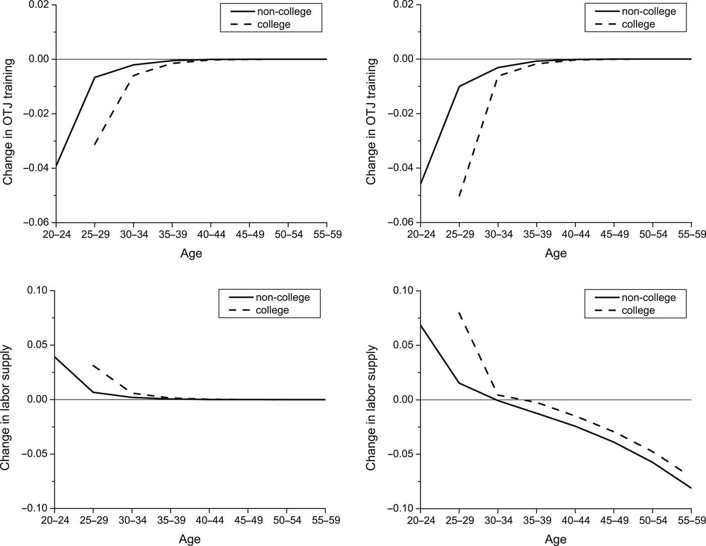
In order to illustrate that, Figure 5 shows changes in on-the-job training investment and labor supply over the life cycle. The reported values are the difference between initial and new long-run equilibrium after the introduction of the accumulation factor. In the upper panels we can clearly see that, in the case of endogenous leisure consumption, the time invested in human capital on-the-job declines further compared to the case with exogenous leisure consumption. This is true for the unskilled (solid line) as well as for college graduates (dashed line). The reason becomes clear from the lower two panels. In case of exogenous leisure consumption, changes in on-the-job training investment are mirrored one to one in the changes of labor supply. Toward the end of the working life where no more human capital formation takes place, labor supply is consequently the same before and after the reform. In the case of endogenous leisure consumption we however find that due to the changes in the implicit tax structure, labor supply declines significantly toward the end of working life and therefore reduces the rental rate of investing in human capital. As a result investment efforts decline further compared to the case with exogenous leisure consumption.
Educational investment and labor supply in the long-run.
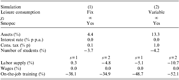
Table 7 reports in the left column selected long-run macroeconomic effects of this reform for the case of exogenous leisure consumption. For now these should be enough to understand the different ingredients of the model and how they are influenced by introducing a positive accumulation factor. I will report transitional dynamics in a later section. As seen above, the introduction of a positive accumulation factor reduces the incentives to invest in human capital through on-the-job training. Therefore the alternative investment strategy, namely investing in the capital market, becomes more favorable and therefore individual assets increase. As aggregate labor supply falls slightly, income tax revenues decline and the consumption tax rate has to increase in the long-run. The negative effect of this reform on college enrollment can be seen in the next row. In this case, the number of students reduces by roughly 5%. As a consequence, we see a shift from high-skilled toward low-skilled labor. This shift overcompensates the reduction in labor supply of the low skilled caused by a decline in human capital investment. Consequently, overall unskilled labor supply slightly increases. The effect on on-the-job training investment is fairly strong. The amount of human capital created through on-the-job investment declines by about 35% for both education groups.
Exogenous vs. endogenous leisure consumption: the macroeconomy
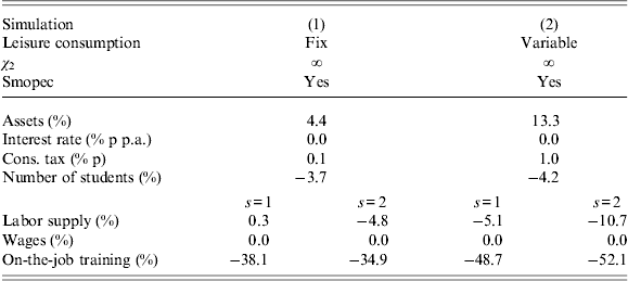
Changes over initial equilibrium values.
In the case of endogenous leisure consumption in the right column of Table 7, the effects are much more pronounced. The main reason for this is that now not only on-the-job training efforts are reduced, but labor supply declines significantly toward the end of the working phase, see Figure 5. Therefore income is even smaller toward later periods in life compared to Simulation (1), which further increases asset accumulation. The stronger increase in consumption taxes can be attributed to the much larger reaction in labor supply. We can still see the shift from high toward low skilled labor. But now, due to the distorting effects of implicit taxes especially toward the end of the working phase, overall labor supply declines for both education groups. Finally, especially on-the-job training efforts are significantly lower compared to the previous simulation, since the fall in labor supply in the later periods of life decreases the incentives to invest in human capital. In terms of college enrollment, the additional reduction in the number of students is rater small.
5.4 Simulation results: factor price reactions
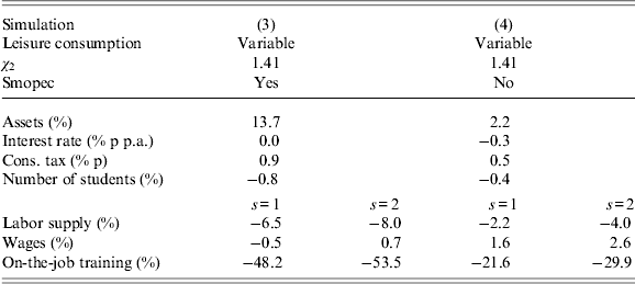
So far, factor prices did not react to changes in individual behavior, since I simulated a small open economy with perfect substitutability of labor. We now want to successively relax these assumptions. When we assume in Simulation (3) in Table 8 that labor of different educational backgrounds is only imperfectly substitutable, the effects on individual assets, consumption taxes and on-the-job training are only tiny. This is not very surprising, since increasing or decreasing the general wage level of an educational group does not have an impact on on-the-job training efforts, as both time costs and returns of human capital investment are equally affected. However, in this simulation we see that the drop in labor supply is much more equal across different educational groups. This stems from the adjustment in wages. As labor supply shifts toward unskilled labor, firms will increase wages for college graduates in order to create an additional incentive for individuals to go through college education. As a result, the number of college graduates rises again (in comparison to the previous simulation) and the shift toward unskilled labor is somewhat mitigated.
Factor price reactions
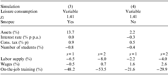
Changes over initial equilibrium values.
If we in addition allow for factor price reactions in the capital market, i.e., assume a closed economy setting, then interest rates will fall in the long run as individual asset holdings increase. This obviously depresses asset accumulation and therefore positively affects human capital investment both through on-the-job training and through going to college. The reason is that the alternative to human capital investment, i.e., investing in the capital market, becomes less attractive. However, the effect on college enrollment is rather small. As labor supply still declines, aggregate wages increase which damps the labor supply reaction in the long-run.
Summing up, we find that the introduction of an accumulation factor of r p,t = r t(1−τ r) in the accumulation equation of the pension system flattens out implicit tax rates over the life cycle and therefore eliminates the positive distortion on human capital formation. The effects are strongest for on-the-job training investment, where the amount of human capital formed through on-the-job training might decline by about 50%. In terms of college education, a reduction in the number of college graduates by roughly 4.5% therefore seems rather modest. Factor price movements will partly counteract these movements, so that interest rates decline and the wage gap between low-and high-skilled individuals increases. Therefore under endogenous factor price reactions, the effects on human capital formation are less pronounced.
5.5 Transitional dynamics
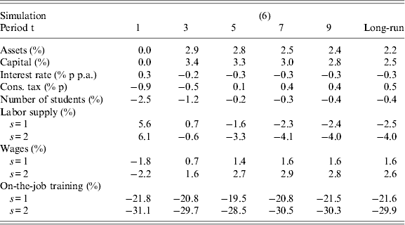
Although comparing long-run equilibrium values was enough to understand the basic mechanics of the model, we now want to look at what happens along the transition. The transitional effects will be crucial for understanding the welfare effects of different cohorts in the next section. Table 9 shows changes in selected variables in the initial transition periods.
Transitional effects of pension funding in general equilibrium
Changes over initial equilibrium values.
Individuals accumulate additional assets quickly in the initial periods of the transition. This is because already in period 1 of the transition less agents decide to invest in human capital both via college education and especially through on-the-job training. Instead, they generate labor income, which they immediately save for later periods in the life cycle. The increase in assets raises productive capital, which again depresses the interest rate and therefore slightly damps asset accumulation in the medium and long run.Footnote 19 Note that the interest rate increases initially, as labor supply rises and therefore capital becomes a scarcer resource. Consumption taxes can be decreased initially due to the increase in labor supply and therefore income taxes. Along the transition, labor supply successively declines, which again increases consumption taxes. As for the college enrollment decision, we find that the decline in the number of students is most pronounced in the initial periods of the transition, as wages only react slowly to the change in educational choices, see below.
In period 1 of the transition, labor supply increases significantly. This results from the fact that individuals now invest less in human capital, but rather spend their time working in the market. Since this decreases labor efficiency of the working population in the medium and long run, labor supply (which is measured in efficiency units) successively reduces throughout the transition. Note that the change in college choice only gradually affects the composition of the work force, since it is only the young cohorts that decide whether to get a college degree or not. The older cohorts already made their college enrollment decision in the initial equilibrium and cannot reverse it. As a result, the shift in labor supply from high toward low skilled labor takes place slowly. The same then obvisouly hold for the wage spread between unskilled and high-skilled workers. Overall wages increase in the medium and long run, since labor supply declines and individuals accumulate more assets. Last but not least, on-the-job training efforts react quickly to the reform and do not vary much afterwards. This is due to the immediate change in implicit tax rates as well as the quick reaction of the interest rate, which stays roughly constant after a couple of periods.
5.6 Welfare effects
With the transitional dynamics at hand, we can now proceed to the welfare effects of the reform. I measure welfare effects along the transition and in the new equilibrium by means of income equivalent variation. Due to the homogeneity of my utility function,
 $$u[(1 + \phi )c_j, (1 + \phi )\ell _j ] = (1 + \phi )^{1 - \gamma} u[c_j, \ell _j ],$$
holds for any  $c_j, \ell _j $ and ϕ. Since utility is additively separable with respect to time, if consumption and leisure were simultaneously increased by the factor 1+ϕ at any age j, life-time utility would increase by the factor (1+ϕ)1−γ. Suppose two agents have the same characteristics z j in the initial equilibrium and the reform year. Let V 0(z j) and V 1(z j) be their corresponding value functions. The income equivalent variation for an individual characterized by z j between living in the initial equilibrium and in the reform year is then given by
 $$\phi = \left\{ {\displaystyle{{V^1 (z_j )} \over {V^0 (z_j )}}} \right\}^{\textstyle{1 \over {1 - \gamma}}} - 1.$$
ϕ indicates the percentage change in both consumption and leisure this individual would require in order to be as well off in the initial equilibrium as in the reform year. Alternatively, I may say that he is ϕ better (or worse) off in terms of resources in the reform year than in the initial equilibrium. If ϕ>0, the reform therefore is welfare improving for this agent and vice versa. A special rule applies to individuals not having entered their economically relevant phase of life in the initial equilibrium (the so-called future generations). I evaluate their utility behind the Rawlsian veil of ignorance, i.e., from an ex-ante perspective where neither their socio-economic background, nor their skill level or any labor market shock has been revealed. The concept of income equivalent variation thereby applies likewise.
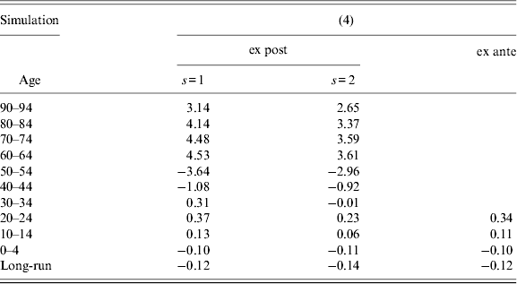
Table 10 shows the welfare effects in the full model with factor price reactions. For generations that were not yet economically active in the initial equilibrium, beneath the ex ante welfare change I also report ex post welfare changes of the unskilled and the skilled. Cohorts are named by their age at the date of the reform t = 1. The cohort ∞ shows welfare effects in the new long-run equilibrium.
Welfare effects of pension funding
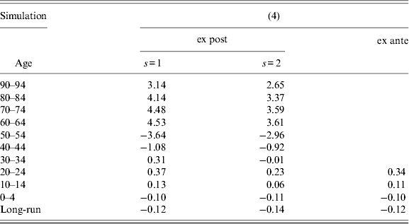
Change in percent of initial resources.
Clearly, the reforms trigger some intergenerational redistribution. On the one hand, retired cohorts gain up to 4.5% of their remaining lifetime resources. This can be attributed mostly to the initial increase in labor supply. As pension payments are indexed to average labor income, an increase in labor supply causes a one to one increase in pension payments. Furthermore, consumption taxes decline at the beginning of the transition and interest rates increase. This again has a positive income effect on retirees. The difference between high-skilled and low-skilled individuals is due to the fact, that college graduates are much more likely to earn income above the cap value of twice the average income. If this is the case, their pension will be over-proportionally smaller than that of a lower skilled agent. Therefore changes in the size of pension payments affect their income relatively less.
For the working age cohorts, the picture looks very different. Especially the generations near to retirement face a significant welfare loss of up to 3.6% from this reform. The reason for this becomes clear when we recall that implicit tax rates for these generations were negative before the reform and immediately jump up to about 10% in the reform year. This triggers a major welfare loss for the elder working generations. Obviously, the younger a generation, the lower the welfare loss up to the point where implicit tax rates actually decrease from the reform. The youngest cohorts therefore obviously experience welfare gains. In the case of the younger cohorts, we can now also see the redistributive effects of the reform experiment. From going over to a flat implicit tax structure, the implicit subsidy to college graduates that caused the number of college students to be higher in the initial equilibrium vanishes. Therefore the positive welfare effects for young cohorts are significantly stronger for the low skilled than for the higher skilled. Throughout the transition, this difference is almost entirely mitigated by the increase in the wage spread between low-and high-skilled individuals. Finally, welfare successively declines throughout the transition and is (only slightly) negative for cohorts born in the new long-run equilibrium.Footnote 20
5.7 Sensitivity analysis
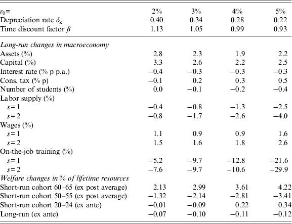
Finally, I want to check the sensitivity of my results with respect to the initial equilibrium interest rate. For this sake I calibrate several initial equilibria with interest rates between 2 and 5% per year. In order to achieve this, I adjust the depreciation rate on capital. Since individual savings behavior is very sensitive to such large changes in the interest rate, I also adapt the time discount factor β in order to obtain the same capital to output ratio. Starting from these different equilibria, I do the same reform experiment as in the previous sections, i.e., set the accumulation factor in the pension system to the net interest rate in the capital market and therefore generate an age independent implicit tax structure.
Table 11 reports the long-run changes in macroeconomic variables as well as selected welfare effects for the short and the long run. Whereas the changes in savings behavior and therefore in the interest rate seem to be almost unaffected, we certainly see differences in the reactions of college enrollment, labor supply, wages and on the job training. This is not surprising. The smaller is the initial equilibrium interest rate, the smaller is the difference between the net return on savings and both the accumulation factor in the pension system (r p = 0) as well as its internal rate of return. This has two consequences for implicit tax rates. First of all, as the difference between the return on capital and the internal rate of return shrinks, implicit tax rates in general decline. Second, since the difference to the accumulation factor falls, the age difference in implicit tax rates decreases, i.e., the implicit tax curve becomes flatter already in the initial equilibrium. The same reform as in the previous section then obviously triggers smaller effect on both college enrollment and on-the-job training and therefore labor supply and wages. In terms of welfare I find that lower initial equilibrium interest rates limit the amount of intergenerational redistribution triggered by the reform. The long-run welfare effect however is hardly impacted.
Sensitivity analysis
6 Conclusion
In this paper, I show that pension systems that calculate pension entitlements with an accumulation factor that is lower than the net capital market interest rate subsidize human capital formation both via college education and via on-the-job training. The reason for that is the implicit tax structure that comes along with such a system. When pension claims are accumulated with a (probably fictitious) interest rate factor that is lower than the capital market interest rate, implicit taxes in the pension system are decreasing with age. When the costs of investing in human capital are mainly time costs, such an implicit tax structure reduces the costs and increases the yield from investing in human capital, since these investments tend to take place in early years of the life cycle. The fact that higher skilled workers tend to have steeper wage profiles over the working phase than the unskilled enforces this mechanism. After showing this result in a simple model, I quantify the effects of getting rid of this incentive effect in a large-scale quantitative OLG model. In order to do so, one has to introduce an accumulation factor for pension claims that is equal to the net interest rate of the economy. Doing this, the implicit tax structure of the pension system becomes flat over the entire working years of the household.
My simulations, which include full transitional dynamics, indicate that in the long-run the effect of flattening out the implicit tax structure of the pension system on college enrollment of households is rather modest. The reason is that, if labor of different educational types is not perfectly substitutable, the wage spread between unskilled and college workers increases, therefore bringing back people into college. However, the impact on on-the-job training is remarkable. There human capital investments are reduced by 20 to up to 50%, depending on whether the economy is of closed or small open type. Labor supply declines by around 3% on average and partly shifts from high to low-skilled labor. In the short run, however, when wages of different skill classes are not yet adjusted to the new situation, the number of college students decreases by roughly 2.5%. Short-run labor supply however increases, since fewer individuals participate in educational measures.
In terms of welfare, a reform that flattens out the implicit tax structure of the pension system comes along with a lot of intergenerational redistribution. Since labor supply increases in the short run and consumption taxes on the other hand decline, retirees that were already living in the initial equilibrium are the big winners from such a reform. Their welfare may increase by about 4.5% of their remaining life-time resources. Older workers, yet, are losing quite significantly, since under the old implicit tax structure their labor supply was subsidized, while under the new system it is taxed at about a 10% rate. Young generations, and especially the non-college population therein, slightly gain from the reform, as the redistributive effect of the pension system toward college graduates is eliminated. In the long-run, however, this positive effect for the unskilled is almost mitigated through reactions in wages.
My results give rise to reconsidering the role of the pension system. In addition, they can have a significant impact on its design. When it comes to the question of redistribution in a pension system, the classical discussion of insurance effects vs. labor supply distortions should certainly be extended to the area of human capital accumulation. Furthermore, as shown above, a perfectly earnings related pension system pays an implicit skill premium and therefore most likely increases inequality. Therefore it might be interesting to look at whether a complementary Beveridgean pillar could counteract this redistributive issue. Last but not least one could test the sensitivity of my results with respect to an endogenous retirement decision. Since flattening out the implicit tax structure of the pension system raises implicit tax rates in the later periods of working life, such a reform decreases the opportunity costs of retiring. Therefore it might induce individuals to retire earlier, which in turn would enforce the negative effects on human capital formation.
Appendix A Computations for the small analytical model
(i) The present value budget constraint
Combining the three dynamic budget constraints yields the standard present value budget constraint
 $$\eqalign{c_1\! + \displaystyle{{c_2} \over {1 + r}} + \displaystyle{{c_3} \over {(1 + r)^2}} = [1 + {\rm {\cal I}}(s)(\pi s - \varpi )]w(1 - \tau ) + \displaystyle{{[1 + {\rm {\cal I}}(s)\pi s\epsilon _2 ]w(1 - \tau )} \over {1 + r}} + \displaystyle{{\,p_3} \over {(1 + r)^2}}. $$
Plugging the definition of p 3 in equation (1) into the LHS of this constraint gives us
 $$\eqalign{& [1 + {\rm {\cal I}}(s)(\pi s - \varpi )]w(1 - \tau ) + \displaystyle{{[1 + {\rm {\cal I}}(s)\pi s\epsilon _2 ]w(1 - \tau )} \over {1 + r}} \cr &\quad + \displaystyle{{\rho (r_p, n)\tau w\{ [1 + {\rm {\cal I}}(s)(\pi s - \varpi )](1 + r_p )^2 + [1 + {\rm {\cal I}}(s)\pi \epsilon _2 ](1 + r_p )\}} \over {(1 + r)^2}} \cr & = [1 + {\rm {\cal I}}(s)(\pi s - \varpi )]w\left( {1 - \tau + \tau \rho (r_p, n)\displaystyle{{(1 + r_p )^2} \over {(1 + r)^2}}} \right) \cr &\quad+ \displaystyle{{[1 + {\rm {\cal I}}(s)\pi s\epsilon _2 ]w\left( {1 - \tau + \tau \rho (r_p, n)\displaystyle{{1 + r_p} \over {1 + r}}} \right)} \over {1 + r}} \cr & = [1 + {\rm {\cal I}}(s)(\pi s - \varpi )]w[1 - \tau _1 (r_p, n)] + \displaystyle{{[1 + {\rm {\cal I}}(s)\pi s\epsilon _2 ]w[1 - \tau _2 (r_p, n)]} \over {1 + r}}} $$
with
 $$\tau _1 (r_p, n) = \tau \left[ {1 - \rho (r_p, n) \cdot \left( {\displaystyle{{1 + r_p} \over {1 + r}}} \right)^2} \right]\quad {\rm and}\quad \tau _2 (r_p, n) = \tau \left[ {1 - \rho (r_p, n) \cdot \displaystyle{{1 + r_p} \over {1 + r}}} \right].$$
(ii) The critical value of s*
The critical value of s* is defined by the equality
 $$\eqalign{& [1 + (\pi s^* - \varpi )]w[1 - \tau _1 (r_p, n)] + \displaystyle{{[1 + \pi s^*\epsilon _2 ]w[1 - \tau _2 (r_p, n)]} \over {1 + r}} \cr & = w[1 - \tau _1 (r_p, n)] + \displaystyle{{w[1 - \tau _2 (r_p, n)]} \over {1 + r}} \cr & \Leftrightarrow(\pi s^* - \varpi )[1 - \tau _1 (r_p, n)] + \displaystyle{{\pi s^*\epsilon _2 [1 - \tau _2 (r_p, n)]} \over {1 + r}} = 0 \cr & \Leftrightarrow \pi s^* + \displaystyle{{\pi s^*\epsilon _2} \over {1 + r}} \cdot \displaystyle{{[1 - \tau _2 (r_p, n)]} \over {[1 - \tau _1 (r_p, n)]}} = \varpi \cr & \Leftrightarrow s^* = \displaystyle{{\varpi /\pi} \over {1 + \displaystyle{{\epsilon _2} \over {1 + r}}\displaystyle{{[1 - \tau _2 (r_p, n)]} \over {[1 - \tau _1 (r_p, n)]}}}}} $$
(iii) Proof or Proposition 2
From the budget constraint of the pension system, we obtain
 $$\eqalign{& \mathop \int \limits_{s \in [0,1]} \rho (r_p, n)\tau w\{ \left[ {1 + {\rm {\cal I}}(s)(\pi s - \varpi )} \right](1 + r_p )^2 + \left[ {1 + {\rm {\cal I}}(s)\pi s\epsilon _2} \right](1 + r_p )\} \; ds \cr &\quad = w\tau \left[ {\displaystyle{{N_1} \over {N_3}} \mathop \int \limits_{s \in [0,1]} 1 + {\rm {\cal I}}(s)(\pi s - \varpi )\; ds + \displaystyle{{N_2} \over {N_3}} \mathop \int \limits_{s \in [0,1]} 1 + {\rm {\cal I}}(s)\pi s\epsilon _2 \; ds} \right],} $$
which we can reformulate to
 $$\eqalign{& \rho (r_p, n)\left\{ {\left[ {1 + \displaystyle{\pi \over 2}(1 - s^{*2} ) - \varpi (1 - s^*)} \right](1 + r_p )^2 + \left[ {1 + \displaystyle{{\pi \epsilon _2} \over 2}(1 - s^{*2} )} \right](1 + r_p )} \right\} \cr & = (1 + n)^2 \left[ {1 + \displaystyle{\pi \over 2}(1 - s^{*2} ) - \varpi (1 - s^*)} \right] + (1 + n)\left[ {1 + \displaystyle{{\pi \epsilon _2} \over 2}(1 - s^{*2} )} \right],} $$
and therefore get the replacement rate of the pension system
 $$\rho (r_p, n) = \displaystyle{{L_1 (1 + n)^2 + L_2 (1 + n)} \over {L_1 (1 + r_p )^2 + L_2 (1 + r_p )}} = \displaystyle{{(1 + n)^2 + \displaystyle{{L_2} \over {L_1}} (1 + n)} \over {(1 + r_p )^2 + \displaystyle{{L_2} \over {L_1}} (1 + r_p )}}$$
with
 $$L_1 = 1 + \displaystyle{\pi \over 2}(1 - s^{*2} ) - \varpi (1 - s^*)\quad {\rm and}\quad L_2 = 1 + \displaystyle{{\pi \epsilon _2} \over 2}(1 - s^{*2} ),$$
denoting non-normalized aggregate labor supply of cohort 1 and cohort 2, respectively. Note that  $\displaystyle{{L_2} \over {L_1}} \geqslant 1$, where equality only holds if ϖ = 0 and ∊2 = 1. The average internal rate of return then is the interest rate that equates the present value of aggregate pension contributions and aggregate payments, i.e., the interest rate i for which
 $$\displaystyle{1 \over {(1 + i)^2}} \cdot \rho (r_p, n)\left\{ {L_1 (1 + r_p )^2 + L_2 (1 + r_p )} \right\} = L_1 + \displaystyle{{L_2} \over {1 + i}},$$
holds. Plugging the replacement rate into this equation, we receive
 $$L_1 (1 + n)^2 + L_2 (1 + n) = L_1 (1 + i)^2 + L_2 (1 + i),$$
and therefore i = n, regardless of the factor r p.
(iv) Proof of Proposition 3
The individual internal rate of return for the unskilled i nc is the interest rate that equates the present value of pension benefits of an unskilled worker with that of his pension contributions. It is therefore defined as
 $$\eqalign{& 1 + \displaystyle{1 \over {1 + i_{nc}}} = \displaystyle{1 \over {(1 + i_{nc} )^2}} \cdot \rho (r_p, n)\left[ {(1 + r_p )^2 + 1 + r_p} \right] \cr & \Leftrightarrow (1 + i_{nc} )^2 + (1 + i_{nc} ) = \rho (r_p, n)\left[ {(1 + r_p )^2 + 1 + r_p} \right] \cr & = \left[ {(1 + n)^2 + \displaystyle{{L_2} \over {L_1}} (1 + n)} \right]\displaystyle{{(1 + r_p )^2 + 1 + r_p} \over {(1 + r_p )^2 + \displaystyle{{L_2} \over {L_1}} (1 + r_p )}}.} $$
From this equation we can directly see that we get i nc = n for L 1 = L 2, i.e., for a case in which there are no time costs ϖ = 0 and no additional wage premium in the second period ∊2 = 1.
Furthermore, we can derive the right-hand side of this equation with respect to r p under the assumption of a constant college enrollment decision. We then obtain
 $$\eqalign{& \displaystyle{{\partial RHS} \over {\partial r_p}} \bigg|_{s^* = const.} = \left[ {(1 + n)^2 + \displaystyle{{L_2} \over {L_1}} (1 + n)} \right] \cr & \cdot \displaystyle{{\left[ {(1 + r_p )^2 + \displaystyle{{L_2} \over {L_1}} (1 + r_p )} \right] \cdot \left[ {2(1 + r_p ) + 1} \right] - \left[ {(1 + r_p )^2 + (1 + r_p )} \right] \cdot \left[ {2(1 + r_p ) + \displaystyle{{L_2} \over {L_1}}} \right]} \over {\left[ {(1 + r_p )^2 + \displaystyle{{L_2} \over {L_1}} (1 + r_p )} \right]^2}} \cr & = \left[ {(1 + n)^2 + \displaystyle{{L_2} \over {L_1}} (1 + n)} \right] \cdot \displaystyle{{(1 + r_p )^2 \cdot \left( {\displaystyle{{L_2} \over {L_1}} - 1} \right)} \over {\left[ {(1 + r_p )^2 + \displaystyle{{L_2} \over {L_1}} (1 + r_p )} \right]^2}} \geqslant 0.} $$
Note that in this case the equality only holds if L 2 = L 1, i.e., there are no time costs of education and there is no additional wage premium in period 2 for going to college. Hence, for L 2 > L 1 we have the right-hand side of equation (27) monotonously increasing in r p and therefore obviously
 $$\displaystyle{{\partial i_{nc}} \over {\partial r_p}} |_{s^* = const.} \gt 0,$$
must hold.